Remote Sensing-Guided Sampling Design with Both Good Spatial Coverage and Feature Space Coverage for Accurate Farm Field-Level Soil Mapping

Abstract

With the increasing requirements of precision agriculture for massive and various kinds of data, remote sensing technology has become indispensable in acquiring the necessary data for precision agriculture. Understanding the spatial variability of a target soil variable (i.e., soil mapping) is a critical issue in solving many agricultural problems. Field sampling is one of the most commonly used technologies for soil mapping, but sample sizes are restricted by resources, such as field labor, soil physicochemical analysis, and funding. In this paper, we proposed a sampling design method with both good spatial coverage and feature space coverage to achieve more precise spatial variability of farm field-level target soil variables for limited sample sizes. The proposed method used the super-grid to achieve good spatial coverage, and it took advantage of remote sensing products that were highly correlated with the target soil property (SOM content) to achieve good feature space coverage. For the experiments, we employed the ordinary kriging (OK) method to map the soil organic matter (SOM) content. The different sized super-grid comparison experiments showed that the 400 × 400 m² super-grid had the highest SOM content mapping accuracy. Then, we compared the proposed method to regular grid sampling (good spatial coverage) and k-means sampling (good feature space coverage), and the experimental results indicated that the proposed method had greater potential in the selection of representative samples that could improve the SOM content mapping accuracy.

1. Introduction

Precision agriculture is a new trend in modern agricultural practices as a way to improve yields and quality, thereby increasing the benefits to farmers and guaranteeing sufficient environmental protection [1,2,3,4,5]. More elaborate soil mapping that reflects the spatial variability of a target soil variable is required to solve various precision agriculture problems, such as soil quality evaluations, soil erosion risk mapping, and variable-rate fertilization [2,6,7,8,9].

The design of the soil survey is a necessary step in producing farm soil maps, including field sampling, laboratory analysis, and data processing [10,11,12,13]. Field sampling, which is a critical issue in soil surveys, helps to obtain reliable soil mapping results by optimizing the sample size and recognizing the representative sampling locations [14,15,16]. Extensive sampling methods have been developed for soil mapping, ranging from simple random sampling to complex, advanced sampling [14,17,18,19,20,21,22,23,24,25,26,27,28,29,30,31,32]. These sampling methods can be classified into three types: geometric sampling (such as grid sampling [30,31] and spatial coverage sampling [20]), adapted experimental sampling (such as conditional Latin hypercube sampling [26] and response surface sampling [33]), and model-based sampling (such as kriging model sampling [14]). In the existing sampling methods, the focus is mainly on two aspects that improve farm soil mapping accuracy: sample size and sample locations [14,34]. It is known that more samples can result in more reliable soil maps, regardless of the sampling methods [35]. However, in most cases, the sample size is determined by available resources, such as field labor, soil physicochemical analysis, and funding [11,15,36]. When the sample size is limited by the available resources and cannot meet the requirements of the precision constraints, the determination of the representative sample locations will become critical to obtaining more accurate soil maps. Additionally, the recognition of representative samples is likely to reduce the sample size since it helps to eliminate the non-representative samples. The study by An et al. [19] indicated that soil mapping results using representative samples had comparable accuracies to conclusions that were produced using full samples.

Sampling design can provide a blueprint for selecting representative sample locations and producing reliable inputs for soil mapping [37]. Most proposed sampling designs in soil mapping create good spatial coverage on one region or good feature space coverage of the covariates for the target soil attribute [11,16,26,30,38,39]. Meanwhile, most studies have improved the efficiency of alternative sampling designs using a given mapping method [40,41,42,43,44,45]. For example, Heuvelink et al. [45] optimized sample locations using spatial simulated annealing for kriging with an external drift. If we use machine learning methods to produce soil maps, good spatial coverage may not be vital compared to good coverage of the environmental covariates [26]. However, accurate interpolation results using the sample data are very dependent on good geographic dispersion [43]. Nevertheless, in many situations, we may not have determined the mapping method when implementing the sampling designs. Thus, it is essential to develop a sampling design that is robust against deviations in modeling assumptions. A sampling design that considers both good spatial coverage and feature space coverage may be a reliable alternative to solve this issue.

Remote sensing technology can be objective and accurate enough to provide sufficient information that is highly correlated with the target farm soil properties, including the normalized difference vegetation index (NDVI), crop yield estimations, the leaf area index (LAI), and the digital elevation model (DEM). For one farm field, the crop yield, NDVI, and LAI are intuitive reflections of soil fertility, since good soil fertility often corresponds to high crop yield, the NDVI, and LAI. Remote sensing crop yield estimation is also a vital issue in precision agriculture. Traditional crop yield estimation technologies use agro-meteorological models, or they analyze the relationship between remote sensing spectral bands or vegetation indexes (such as NDVI, EVI, GVI, SAVI, and LAI) and the field-measured yields to forecast the crop yield in large agricultural regions [46,47,48,49,50,51,52,53]. However, these methods are restricted by specific crop cultivars, crop growth stages, and geographical regions [54,55]. Crop models, such as the CERES-Wheat model [56], the WOFOST model [55,57,58], and the SWAP (soil–water–atmosphere–plant) model [59], are good alternatives to solve the above problems since they can simulate key physical, physiological, and soil processes, and they fully consider issues such as abnormal weather conditions and natural disasters [60]. Thus, in recent years, the integration of remote sensing technology and crop models has been the focus of crop yield estimation research [54,57,61,62]. For example, Cheng et al. [54] developed a simple yet effective method with fast algorithms to assimilate the time-series HJ-1 A/B data into the WOFOST model, and the results demonstrated that the proposed method could improve spring maize yield simulations. meanwhile, the DEM can partly explain soil erosion and diffusion [38]. These remote sensing products are helpful in discerning representative sample locations with good feature space coverage [63,64]. Thus, we could use these products to optimize sample locations to achieve good feature space coverage when the samples are also geographically well dispersed.

In this paper, we proposed a sampling design method considering both good spatial coverage and feature space coverage to improve farm field-level soil mapping accuracy with limited sample sizes. First, the proposed method determined the optimal super-grid space by analyzing the influence of different sized super-grid spaces on soil mapping accuracy, and then, this was compared to regular grid sampling (good spatial coverage) and k-means sampling (good feature space coverage) using visual and quantitative analysis of the soil mapping. The ordinary kriging (OK) method was employed for farm field-level soil organic matter (SOM) mapping.

2. Material and Methods

2.1. Study Area and Dataset

The study area was Sheltara Farm, which is located in the northeast part of the Nei Monggol Autonomous Region, China, where it covers an area of 595 km² (Figure 1). Sheltara Farm intensively exploits arable land, and commonly cultivated crops in this area include wheat, barley, rape, silymarin, and potatoes. Due to climate limitations, the area’s cropping system is “one crop a year.” Crops are planted in May and harvested in September. The elevation ranges from 488 to 771 m, and the central and eastern areas have a relatively high relief. The climate is windy and rainless in spring, and it has concentrated precipitation in the summer, with a rapid cooling and early frost in the autumn, as well as a long duration of cold and snow cover in the winter. The average annual temperature ranges from −5.9 to 5.9 °C, and the average annual precipitation ranges from 125 to 542 mm.

Farm field SOM content mapping was the main target of this paper, and the tested field was 70.2 ha in size. As a way to validate the proposed sampling design method, all the sampling and validation points were the extracted values from one SOM map during the autumn of 2018, which we used as the ground truth. The SOM map was obtained from the local soil experts of Sheltara Farm. Note that the local soil experts collected 883 soil samples over the whole area of Sheltara Farm in the autumn of 2018 to obtain the spatial distribution of the SOM content of the whole farm, and to form the cultivation plan for the next year. The SOM map of Sheltara Farm was produced using the ordinary kriging (OK) method and the 883 collected soil samples. The SOM content of these 883 soil samples ranged from 28.71 to 65.54 g/kg, and the mean and standard deviation were 44.59 g/kg and 7.38 g/kg, respectively. The prediction errors of the SOM mapping for the whole farm are displayed in

Table 1. The prediction errors of the soil organic matter (SOM) mapping of the whole farm and the descriptive statistics of the tested farm field SOM map.

The Prediction Errors of the SOM Mapping of the Whole Farm
Mean (g/kg)	Root-Mean-Square (g/kg)	Mean Standardized (g/kg)	Root-Mean-Square Standardized (g/kg)		Average Standard Error (g/kg)
0.08	5.42	0.02	0.79		6.79
The Descriptive Statistics of the Tested Farm Field SOM Map
SOM Content	Min (g/kg)	Max (g/kg)	Median (g/kg)	Mean (g/kg)	Standard Deviation (g/kg)
Tested field	42.86	44.75	43.94	43.89	0.45

. Subsequently, the SOM map of the tested farm field was clipped from the predicted SOM map of the whole farm, and it was used as the ground truth to test the proposed sampling design method. The descriptive statistics of the tested farm field SOM map are shown in Table 1.

The digital elevation model (DEM), slope, aspect, and crop yield could partly explain the spatial variation of the SOM content; thus, these four environmental variables were used to optimize the sample locations in the feature space.

Table 2. The dataset characteristics of the tested field.

Dataset	Spatial Resolution	Time
Soil organic matter (SOM) map	Raster, 16 m	2018
Digital elevation model (DEM)	Raster, 16 m	2009
Slope	Raster, 16 m	2009
Aspect	Raster, 16 m	2009
Remote sensing crop yield data	Raster, 16 m	2018

displays the information on the SOM map taken in the autumn of 2018 and the four environment variables in detail. The DEM data with a 30 m resolution was downloaded from the Geospatial Data Cloud website (http://www.gscloud.cn/). For consistency with the resolution of the crop yield data, the DEM data was resampled to 16 m using the nearest neighbor assignment algorithm. The slope and aspect were calculated based on the resampled DEM data using the 3D Analyst Tools in ArcGIS 10.2. The crop yield data in 2018 was from the Aerospace Information Research Institute, Chinese Academy of Sciences. The remote sensing crop yield data was produced by Meng Group using the WOFOST Model [54].

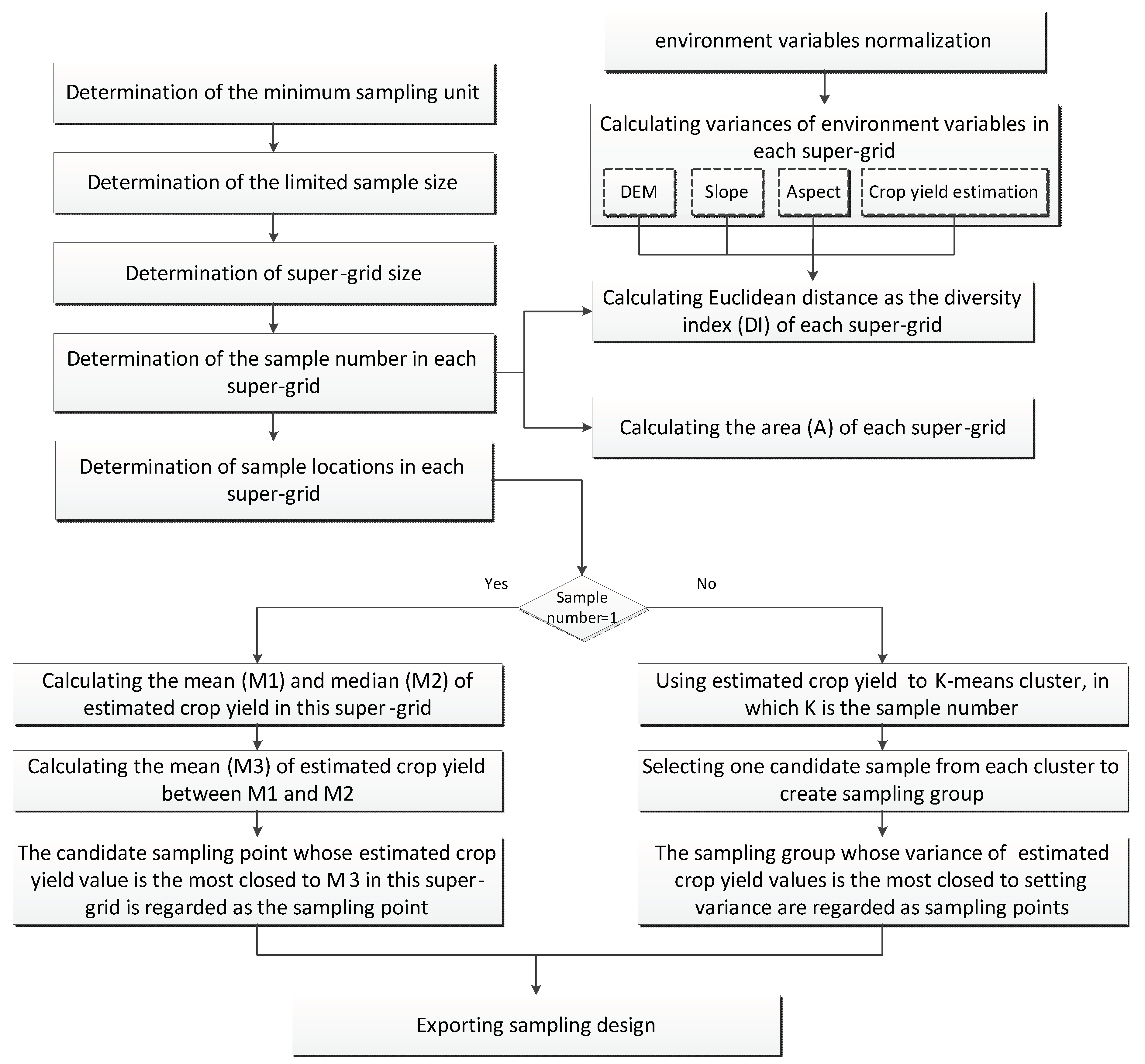
2.2. Sampling Design Method Considering Both Good Spatial Coverage and Feature Space Coverage

The process of the proposed sampling design method could be described as follows. First, the minimum sampling unit, sample size, and super-grid size were determined. Second, the diversity index and area in each super-grid were calculated to determine the number of samples in every super-grid. Third, the sample locations were determined in each super-grid. The schematic of the proposed method is displayed in Figure 2.

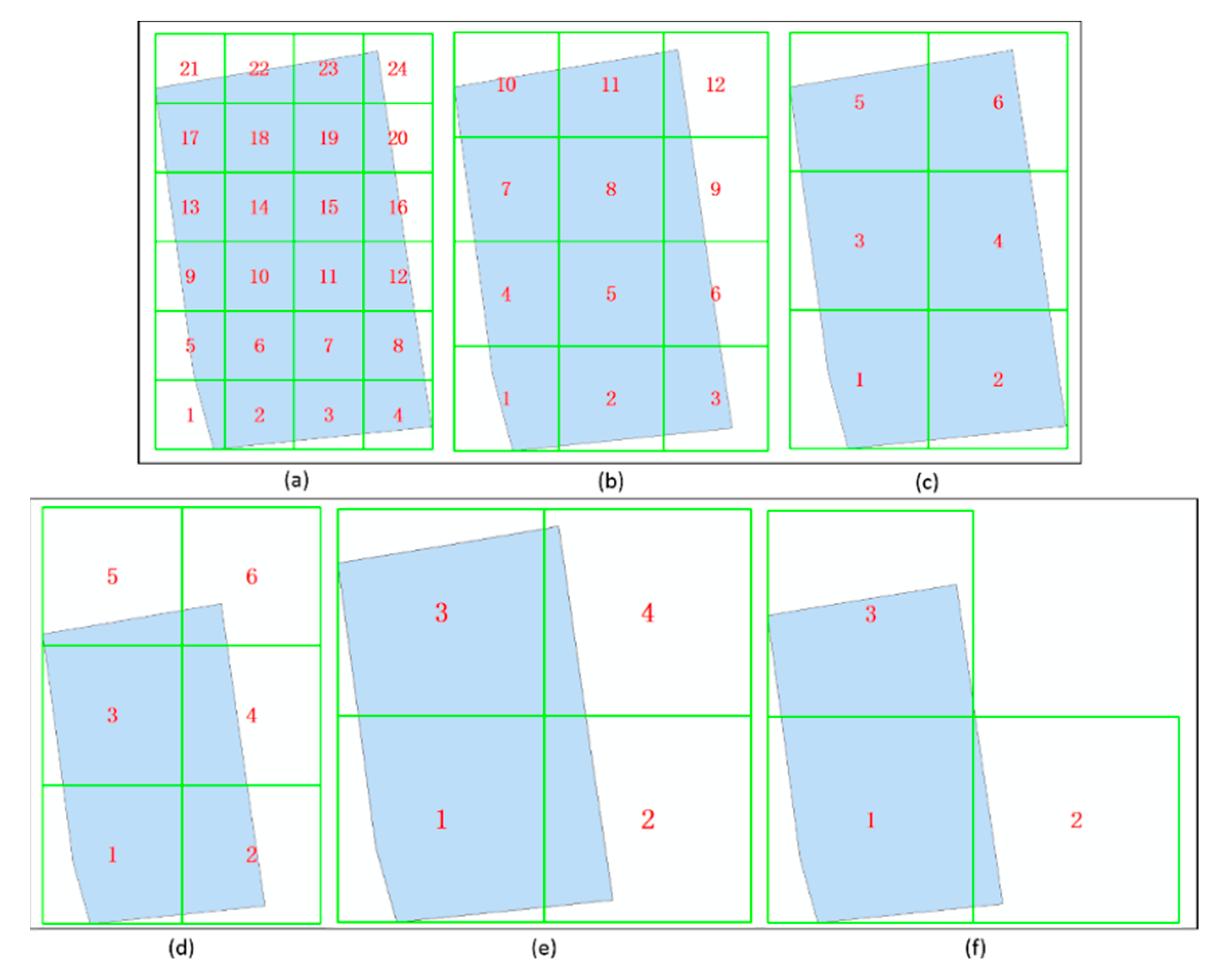
2.2.1. Determination of the Minimum Sampling Unit, Sample Size, and Super-Grid Size

First, the minimum sampling unit was determined. In this paper, a grid size of $20\times 20$ m² was considered as the minimum sampling unit. Then, the fishnet with the minimum sampling unit was created using the Data Management Tools in ArcGIS 10.2, and the center of each fishnet was recognized as a candidate sampling point. The number of candidate sampling points in this tested field was 1759. Second, the limited sample size was determined. This paper set two percent of the number of candidate sampling points as the limited sample size, i.e., 36 sampling points. Finally, the super-grid size was determined. Note that the super-grid refers to one square region in which the length of its sides is larger than the interval between two candidate sampling points, and it is at least the double interval. To ensure good spatial coverage, one or more sampling points were required to be recognized in each super-grid. Thus, the number of super-grids could not exceed the sample size. In this study, the number of super-grids was between one and 36. In other words, the super-grid size ranged from 140 × 140 m² to $800\times 800$ m². To analyze the influence of super-grid size on sampling design, this paper compared the sampling design results using super-grid sizes of 200 × 200 m², 300 × 300 m², 400 × 400 m², 500 × 500 m², 600 × 600 m², and 700 × 700 m². The approach to create a super-grid was the same as creating the minimum sampling unit, as shown in Figure 3.

2.2.2. Determination of the Number of Sampling Points in Each Super-Grid

To achieve good coverage of feature space, we believed that more sampling points were required if the variation of the environment variables in one local field region was very high. This paper combined the four local variation information of the DEM, slope, aspect, and crop yield to assess the variation of the target soil attribute. First, the values of these four environmental variables were extracted using candidate sampling points using the Spatial Analyst Tools in ArcGIS 10.2. Then, a standardization procedure was applied to the environmental variables using the following formula:

$$\overline{\overline{X_i}}=\frac{X_i-X_{\mathrm{i}\_\min }}{X_{\mathrm{i}\_\max }-X_{\mathrm{i}\_\min }}$$

(1)

where $X_i$ is environmental variable i and $X_{\mathrm{i}\_\min }$ and $X_{\mathrm{i}\_\max }$ are the lowest and highest values of environmental variable i, respectively. Next, the variances of the normalized environmental variables within one super-grid were calculated as follows:

$${\mathrm{v}}_{\mathrm{i}}=\frac{{\displaystyle \sum _{\mathrm{j}=1}^{\mathrm{n}}{({\mathrm{y}}_{\mathrm{i}\mathrm{j}}-\overline{{\mathrm{y}}_{\mathrm{i}}})}^2}}{\mathrm{n}}$$

(2)

where ${\mathrm{y}}_{ij}$ is one of the values of environmental variable i within one super-grid, ${\overline{y}}_i$ is the mean of the values of environmental variable i within the super-grid, and n is the number of candidate sampling points within the super-grid. Finally, the diversity index (DI) of the super-grid was calculated to assess the variation of the target soil attribute as follows:

$$\mathrm{D}\mathrm{I}=\sqrt{{\displaystyle \sum _{\mathrm{i}=1}^{\mathrm{n}}{\mathrm{v}}_i^2}}$$

(3)

where $v_i$ is the variances of normalized environmental variable i within one super-grid. The area of the candidate sampling region in the super-grid is also the non-negligible element for determining the number of samples in the super-grid. In this paper, the number of candidate sampling points in the super-grid was regarded as the area (A). Then, the combination of DI and A was considered to calculate the sample size ($N_k$) in each super-grid, as follows:

$${\mathrm{N}}_{\mathrm{k}}=\mathrm{m}\cdot \frac{{\mathrm{A}}_{\mathrm{k}}\cdot \mathrm{D}{\mathrm{I}}_{\mathrm{k}}}{{\displaystyle \sum _{\mathrm{k}=1}^{\mathrm{n}}{\mathrm{A}}_{\mathrm{k}}\cdot \mathrm{D}{\mathrm{I}}_{\mathrm{k}}}}$$

(4)

where m is the sample size discussed in Section 2.2.1, and $A_k$ and $D{I}_k$ represent the area and diversity index of super-grid k, respectively. Assume that one sampling point is enough to obtain the spatial distribution of the SOM content within one farm field and that one farm has 1000 fields. One sampling point is far from enough to achieve the reliable spatial distribution of the whole farm’s SOM content. More sampling points are required for larger areas. In addition, two regions with the same area have different spatial variations of their SOM contents. The region with a high SOM content variation was called Region1, and the other was called Region2. Region1 required more sampling points than Region2 to obtain satisfactory soil mapping results. The high target variable variation corresponded to a high DI. Thus, more sampling points are necessary for a large area and high target variable variation, wherein this paper used the product of $A_k$ and $D{I}_k$ as the weight to determine the number of samples for super-grid k. Note that the number of sampling points in each super-grid may not be an integer when using Equation (4). In this situation, the number of sampling points is rounded up and should satisfy the condition that at least one sampling point is recognized within one super-grid. Then, the number of sampling points for all the super-grids are summed. If the result is greater than the given sample size (i.e., 36 sampling points), then 36 sampling points are randomly selected from the sampling design after the sampling locations are determined (the detailed information is given in Section 2.2.3). If the result is less than the given sample size, the super-grids with a decimal portion where $N_k$ is less than 0.5 will be ranked based on the decimal portion of $N_{k}s$. The top-ranked super-grid(s) will add one sampling point.

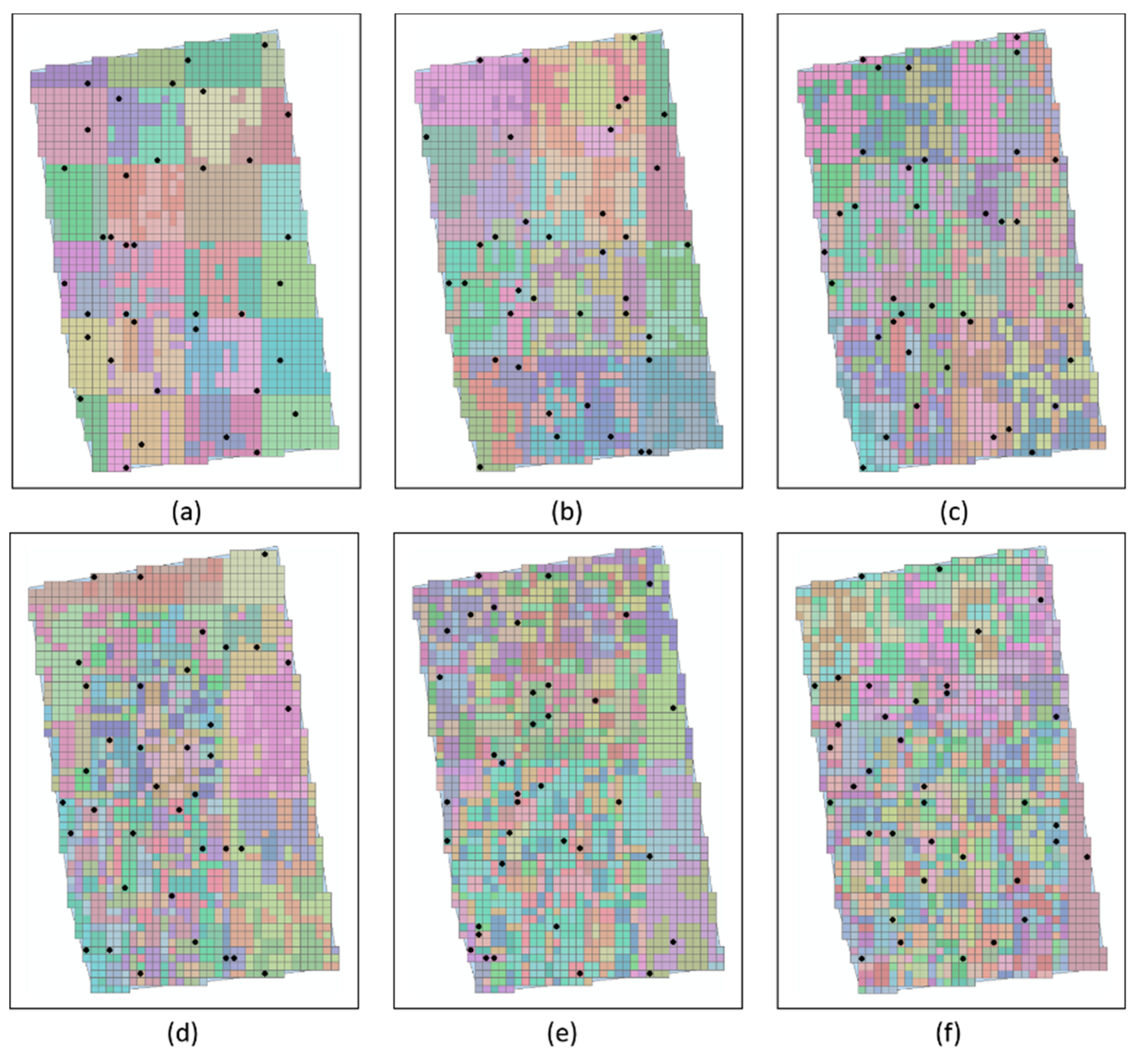
2.2.3. Determination of the Sampling Locations in Each Super-Grid

The SOM content can influence crop growth and fertile accumulation within one super-grid [19]. We do not have a priori knowledge of SOM content before designing soil sampling. To determine the representative sample locations, some remote sensing productions that are highly correlated with the target soil variable were used to help discern representative sample locations. Many studies have shown high correlations between SOM and yield [65,66,67]. The relationship between SOM and yield can be restricted by the interacting factors related to management, climate, and soil type. However, the management of Sheltara farm involves mechanized unified crop cultivation, irrigation and fertilization, and this paper selected one natural field to validate the proposed method for farm field-level soil mapping. The tested field only grows one crop and its soil type is chernozem. It is believed that the climate, temperature, and disaster conditions are similar in a limited field space (i.e., super-grid). Thus, the SOM–yield relationship may have been less affected by the interacting factors related to management, climate, and soil type within one super-grid. In general, high SOM content results in high crop yield, whereas low SOM content leads to low crop yield within one super-grid. Hence, the spatial variation of the crop yield reflect the spatial variation of the farm’s SOM content for a limited field space, since the differences in the soil physio-chemical properties (texture, drainage, SOC, carbonates, etc.) should be minimal in limited field space. The sampling locations could be determined based on the remote sensing crop yield data due to the high correlation between the crop yield and SOM content. First, the k-means algorithm [20,68,69,70] was applied to the environmental variable of the remote sensing crop yield data to generate clusters within each super-grid. The number of clusters was equal to the number of samples within the super-grid. Note that if the number of samples was equal to 1, the operation of k-means clustering would be avoided.

Second, the approach of determining the sample locations within each super-grid could be defined using the following rules. In the case of the number of sampling points being equal to 1, the mean (M1) and median (M2) of the crop yields in each super-grid are calculated, and then the mean (M3) of the crop yields between M1 and M2 is calculated. The candidate sampling point with a crop yield that is closest to M3 within the super-grid is recognized as the sampling point. In the case that the number of sampling points is greater than 1, the variance (v) of the crop yields of all the candidate sampling points within the super-grid is calculated using Equation (2). Then, the desired variance (DV) is calculated using the following formula:

$$\mathrm{D}\mathrm{V}=\frac{\mathrm{v}}{\mathrm{N}}\cdot \mathrm{N}1$$

(5)

where N is the number of sampling points within the super-grid, and N1 is the number of the candidate sampling points within the super-grid. Next, one candidate sampling point is selected from each cluster to create the sampling point groups within the super-grid, and the sampling point group with a crop yield variance that is closest to the DV is regarded as the sampling point of the super-grid. The sampling design of the farm field soil is the output after determination of the sample locations within each super-grid.

2.3. Farm Field Soil Mapping and Evaluation

The ordinary kriging (OK) [26,30,71,72] method was employed to predict the SOM content of the tested farm field. At present, OK is one of the most commonly used geostatistical tools for soil nutrient predictions [30]. In this paper, OK was implemented using the Geostatistical Analyst tool in ArcGIS 10.2.

To validate the proposed sampling design method, we compared it to the regular grid sampling method and the k-means sampling method [16,30]. The former ensures good spatial coverage, while the latter provides good feature space coverage. We applied the mean absolute error (MAE) and root mean square error (RMSE) to test the SOM content maps that were produced by the proposed method, the regular grid sampling method, and the k-means sampling method. The MAE and RMSE can be defined as follows:

$$\mathrm{MAE}=\frac{{\displaystyle \sum _{\mathrm{i}=1}^{\mathrm{n}}\left|{\mathrm{T}}_{\mathrm{i}}-{\widehat{\mathrm{T}}}_{\mathrm{i}}\right|}}{\mathrm{n}}$$

(6)

$$\mathrm{RMSE}=\sqrt{\frac{{\displaystyle \sum _{\mathrm{i}=1}^{\mathrm{n}}{({\mathrm{T}}_{\mathrm{i}}-{\widehat{\mathrm{T}}}_{\mathrm{i}})}^2}}{\mathrm{n}}}$$

(7)

where ${\mathrm{T}}_{\mathrm{i}}$ is the ground truth of the validation sample i, ${\hat{\mathrm{T}}}_{\mathrm{i}}$ is the predicted SOM content value of sample i, and n is the total number of validation samples.

The selection of the validation samples is very critical to obtaining objective evaluation results. The validation samples containing the sampling points will produce higher accuracy for testing the SOM content maps, resulting in a non-objective evaluation [19]. Thus, the sampling points that are determined using the three sampling design methods must be moved from the candidate sampling points before selecting the validation samples. Then, the validation samples are randomly selected from the remaining candidate sampling points. The size of the validation sample is three times as large as the sample size, i.e., 108 validation points. Since the validation samples were randomly chosen, we repeated the selection process 200 times and generated 200 validation sample sets.

3. Results

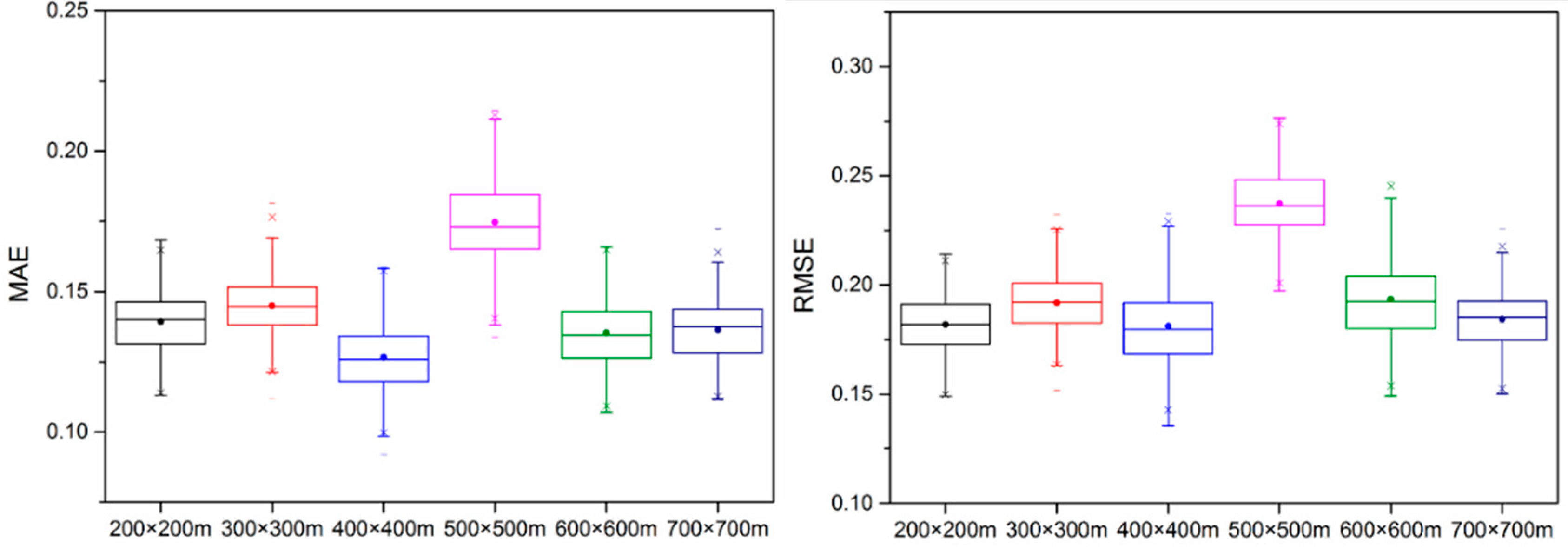
3.1. Analysis of the Influence of Super-Grid Size for the Proposed Sampling Design Method

Since the sample size was restricted by resources, including field labor, soil physicochemical analysis, and funding, this paper proposed a new sampling design method that recognized representative sample locations to improve soil mapping accuracy for a limited sample size (i.e., 36 sampling points in this paper). This method determined the appropriate super-grid size and then assigned the limited sampling points to the super-grids based on the remote sensing data to identify the representative sample locations.

As discussed in Section 2.2.1, this paper compared super-grid sizes of 200 × 200 m², 300 × 300 m², 400 × 400 m², 500 × 500 m², 600 × 600 m², and 700 × 700 m² and analyzed their soil mapping accuracy.

Table 3. The numbers of candidate sampling points ($N_{can}$), the diversity indexes (DIs), and the numbers of sampling points ($N_{sam}$) for the super-grids ranging from 200 × 200 m² to 700 × 700 m².

Super-Grid ID	200 × 200 m2			300 × 300 m2			400 × 400 m2			500 × 500 m2			600 × 600 m2			700 × 700 m2
	${\mathit{N}}_{\mathit{c}\mathit{a}\mathit{n}}$	DI	${\mathit{N}}_{\mathit{s}\mathit{a}\mathit{m}}$	${\mathit{N}}_{\mathit{c}\mathit{a}\mathit{n}}$	DI	${\mathit{N}}_{\mathit{s}\mathit{a}\mathit{m}}$	${\mathit{N}}_{\mathit{c}\mathit{a}\mathit{n}}$	DI	${\mathit{N}}_{\mathit{s}\mathit{a}\mathit{m}}$	${\mathit{N}}_{\mathit{c}\mathit{a}\mathit{n}}$	DI	${\mathit{N}}_{\mathit{s}\mathit{a}\mathit{m}}$	${\mathit{N}}_{\mathit{c}\mathit{a}\mathit{n}}$	DI	${\mathit{N}}_{\mathit{s}\mathit{a}\mathit{m}}$	${\mathit{N}}_{\mathit{c}\mathit{a}\mathit{n}}$	DI	${\mathit{N}}_{\mathit{s}\mathit{a}\mathit{m}}$
1	29	0.04	1	126	0.08	3	273	0.1	6 + 1	471	0.12	12	720	0.11	18	1020	0.1	23
2	93	0.09	2	203	0.1	5	335	0.07	6	302	0.07	5	219	0.06	3	85	0.07	1
3	83	0.09	2	112	0.06	2	341	0.11	9	577	0.1	13	708	0.09	14	654	0.08	12
4	69	0.07	1	166	0.12	5	321	0.06	5	250	0.07	4	112	0.07	2	-	-	-
5	51	0.07	1	225	0.1	5	267	0.08	5	106	0.08	2	-	-	-	-	-	-
6	100	0.12	3	107	0.06	2	222	0.07	4	53	0.05	1	-	-	-	-	-	-
7	100	0.06	2	196	0.08	4	-	-	-	-	-	-	-	-	-	-	-	-
8	83	0.05	1	225	0.08	4	-	-	-	-	-	-	-	-	-	-	-	-
9	64	0.13	2	75	0.07	1	-	-	-	-	-	-	-	-	-	-	-	-
10	100	0.12	3	123	0.07	2	-	-	-	-	-	-	-	-	-	-	-	-
11	100	0.07	2	164	0.06	3	-	-	-	-	-	-	-	-	-	-	-	-
12	67	0.07	1	37	0.05	1	-	-	-	-	-	-	-	-	-	-	-	-
13	77	0.08	2	-	-	-	-	-	-	-	-	-	-	-	-	-	-	-
14	100	0.09	2	-	-	-	-	-	-	-	-	-	-	-	-	-	-	-
15	100	0.05	1	-	-	-	-	-	-	-	-	-	-	-	-	-	-	-
16	54	0.07	1	-	-	-	-	-	-	-	-	-	-	-	-	-	-	-
17	91	0.06	1	-	-	-	-	-	-	-	-	-	-	-	-	-	-	-
18	100	0.09	2	-	-	-	-	-	-	-	-	-	-	-	-	-	-	-
19	100	0.07	2	-	-	-	-	-	-	-	-	-	-	-	-	-	-	-
20	39	0.06	1	-	-	-	-	-	-	-	-	-	-	-	-	-	-	-
21	30	0.08	1	-	-	-	-	-	-	-	-	-	-	-	-	-	-	-
22	46	0.09	1	-	-	-	-	-	-	-	-	-	-	-	-	-	-	-
23	64	0.06	1	-	-	-	-	-	-	-	-	-	-	-	-	-	-	-
24	19	0.05	1	-	-	-	-	-	-	-	-	-	-	-	-	-	-	-

shows the numbers of the candidate samples, the diversity indexes, and the number of sampling points of different sized super-grids. Different super-grid sizes resulted in various DIs and numbers of sampling points within one super-grid. For the 200 × 200 m² super-grid, super-grids 6, 9, and 10 had relatively higher DIs than the others. The number of samples ranged from 1 to 3, and super-grids 6 and 10 had the most samples. For the 300 × 300 m² super-grid, super-grids 2, 4, and 5 had higher DIs and more samples than the others. The number of samples ranged from 1 to 5. For the 400 × 400 m² super-grid, the DIs of super-grids 1 and 3 were relatively higher. Additionally, they had more sampling points. The number of samples varied from 4 to 9. For the 500 × 500 m² super-grid, the super-grids 1 and 3 had higher DIs and a higher number of sampling points compared to the other super-grid IDs. The number of sampling points was from 1 to 13. For the 600 × 600 m² super-grid, super-grid 1 had the highest soil variation, indicated by the highest DI. The number of samples ranged from 2 to 18. For the 700 × 700 m² super-grid, super-grid 1 had relatively higher DIs and the largest area, and thus, its number of sampling points was more compared to the other IDs. The number of sampling points ranged from 1 to 23. As the super-grid size increased, the difference in the number of sampling points between the super-grids increased. It indicated that the spatial coverage gradually worsened, whereas the feature space coverage improved as the super-grid size increased.

By calculating the sum of the numbers of sampling points for all super-grids, the numbers of sampling points within the farm field using super-grids that ranged from 200 to 700 m were 37, 37, 35, 37, 37, and 36, respectively. The reason that some calculated sample sizes were not equal to the given limited sample size (i.e., 36 sampling points) was that the sampling number in each super-grid, as calculated by Equation (4) may not be an integer. According to Section 2.2.2, 36 sampling points were randomly chosen from the sampling design results that were produced by the 200 × 200 m², 300 × 300 m², 500 × 500 m², and 600 × 600 m² super-grids after determination of the sampling locations. For the 400 × 400 m² super-grid, super-grid 1 added one sampling point.

Finally, the sample locations within each super-grid were determined based on the rule described in Section 2.2.3. Figure 4 shows the clustering results based on the crop yield information and the distribution of the sampling points. The distribution of the sampling points of the 200 × 200 m² super-grid provided better spatial coverage compared to distributions of other different sized super-grids. As the super-grid size increased, the good spatial coverage decreased, and the environmental covariate information was given more weight to determine the sample locations.

The purpose of soil sampling is to produce precise SOM content maps. To analyze the impact of the super-grid size on SOM content mapping accuracy, the six groups of sampling points that were generated by the different sized super-grids were input into the ordinary kriging (OK) model. The validation results are displayed in Figure 5. Note that the 108 validation samples were randomly selected after the six groups of sampling points were removed from the candidate sampling points in the farm field, and the process was repeated 200 times. The MAE that was obtained by the 400 × 400 m² super-grid was smaller than the MAE obtained by the other super-grid sizes. The average RMSE that was obtained by the 400 × 400 m² super-grid was the smallest among the six results. Thus, the 400 × 400 m² super-grid generated a higher accuracy compared to the other different sized super-grids, and it was regarded as the optimal super-grid size in this paper.

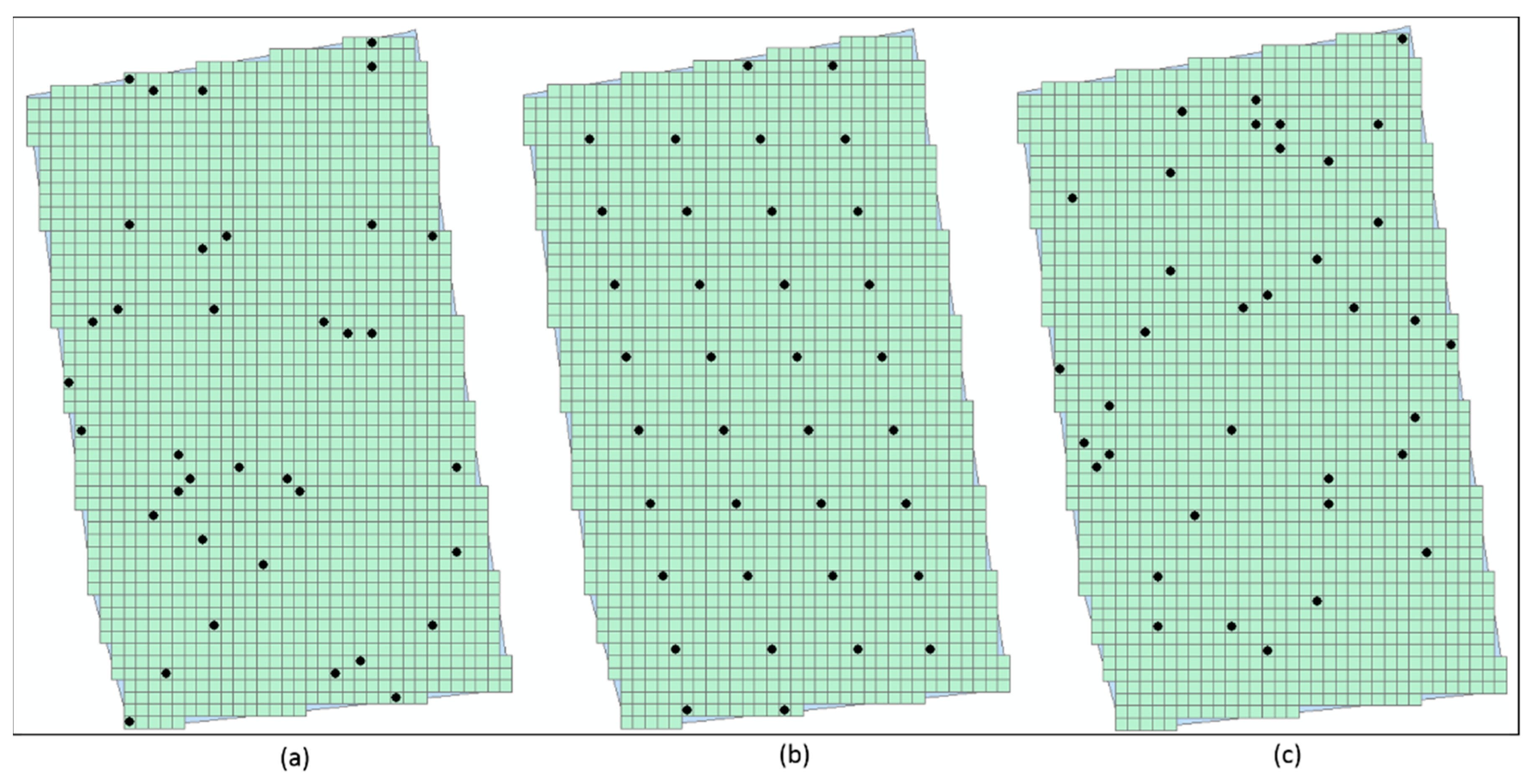
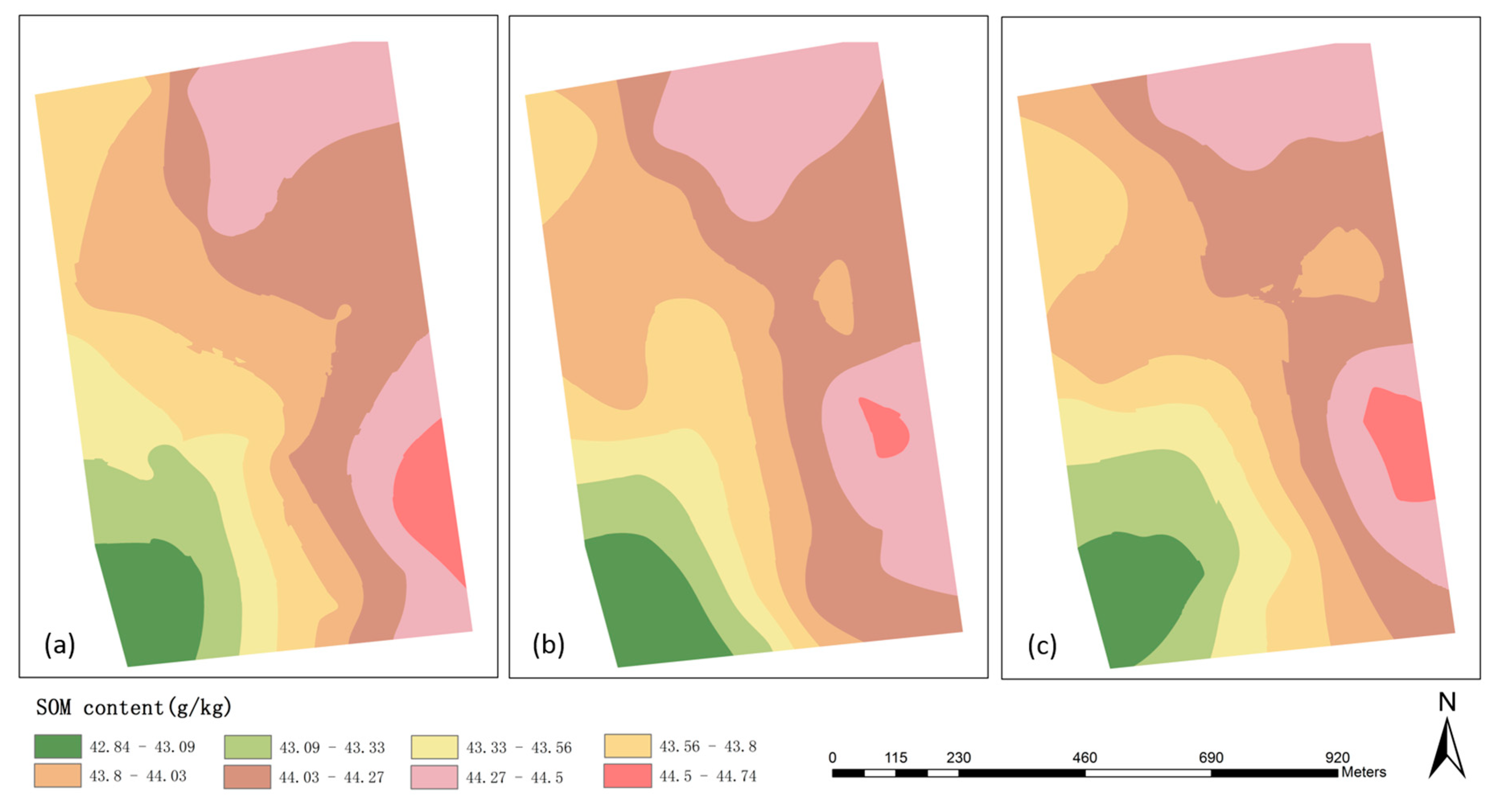
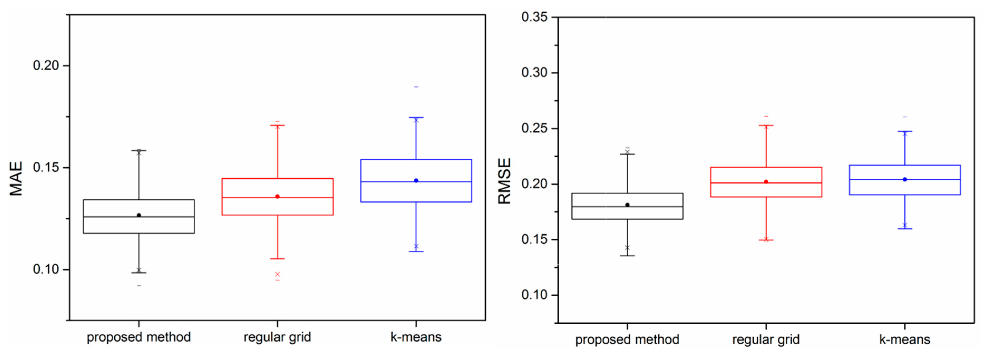
3.2. Comparison to Other Sampling Design Methods for Farm Field Soil Mapping

To demonstrate the effectiveness of the proposed method, the results of the sampling design using the proposed method, the regular grid sampling method, and the k-means sampling method were compared, as shown in Figure 6. Figure 6b shows good spatial coverage, whereas Figure 6c shows good feature space coverage. Compared to Figure 6b,c, Figure 6a shows a better trade-off between good spatial coverage and feature space coverage.

Table 4. The descriptive statistics of the SOM contents of the farm field soil samples that were produced by the three sampling design methods.

Sampling Method	Min (g/kg)	Max (g/kg)	Median (g/kg)	Mean (g/kg)	Standard Deviation (g/kg)
Proposed method	42.86	44.74	43.86	43.81	0.45
Regular grid	42.87	44.51	43.99	43.9	0.44
k-means	42.89	44.51	44.02	43.92	0.44

displays the descriptive statistics of the SOM contents of farm field soil samples that were produced using the three sampling design methods. The sampling points produced by the proposed method had a smaller minimum value and a larger maximum value and standard deviation of the SOM content compared to the values of the other two methods. Moreover, the maximum SOM contents of the sampling points that were generated by the other two methods were significantly smaller than the contents of the proposed method. According to Table 1, the sampling design results generated by the proposed method had similar descriptive statistics with respect to the min, max, and standard deviation of the SOM content using the tested farm field SOM map (the ground truth). It indicated that the sampling points produced by the proposed method seemed to be more representative than the points produced by the other two methods.

To further validate the proposed sampling method, the predicted SOM content maps using the three groups of samples are shown in Figure 7, and the validation results are displayed in Figure 8. The trends in the SOM content variations of these three mapping results were similar. The SOM content was low in the southwest region of the tested farm field, whereas it was high in the northeastern region. In the southeastern region, the SOM content variation of Figure 7a was similar to that of Figure 7c, whereas Figure 7b had a lesser area with large SOM contents. In the middle-eastern part of this farm field, the predicted SOM contents of Figure 7b,c were lower than that of Figure 7a. The quantitative results (Figure 8) showed that the MAE and RMSE of the proposed method were significantly lower than the results of the other two competitive methods. The MAE of the regular grid sampling method was lower than that of the k-means sampling method, whereas the former had a slightly lower RMSE compared to the latter. It indicated that the proposed method was superior to the other two methods and that the regular grid method performed better than the k-means method in the tested farm field.

4. Discussion

With the increasing requirements of precision agriculture for massive and various kinds of data, the data acquisition process has evolved from truth-surveying to sensors [73]. Remote sensing technology can provide a convenient approach to acquire the necessary data for precision agriculture, such as calculating the NDVI and LAI. The accurate determination of spatial variability of the target soil variable is a critical issue in precision agriculture. Thus, the selection of representative soil samples for higher soil mapping accuracy was the main focus of this paper. Traditional farm field soil sampling only considers good spatial coverage, ignoring the impact of good feature space coverage of the covariates on the farm field soil mapping accuracy. Some remote sensing measures, such as the NDVI and crop yield estimations, can explain the variation of the farm field’s target soil variable. These measures can be used as covariates to recognize the representative soil samples for good feature space coverage. In this paper, we collected the crop yield data produced using the WOFOST model, DEM, slope, and aspect as the covariates. In the future, we will explore the potential use of more remote sensing measures for farm field soil sampling, such as gross primary production (GPP) and LAI.

This paper developed a sampling design method considering both good spatial coverage and feature space coverage for farm field-level soil mapping. Good feature space coverage can be achieved by assessing the aforementioned remote sensing measures. In this paper, good spatial coverage was achieved using the super-grid. However, the selection of the appropriate super-grid size is important in forming a satisfactory sampling design. Thus, this paper compared the influence of six different super-grid sizes (i.e., 200 × 200 m², 300 × 300 m², 400 × 400 m², 500 × 500 m², 600 × 600 m², and 700 × 700 m²) on the soil mapping accuracies. Figure 5 shows that the soil mapping accuracy of the 400 × 400 m² super-grid was the highest, as indicated by the lowest MAE and average RMSE. A possible reason may be that the 400 × 400 m² super-grid balanced the potential trade-offs between good spatial coverage and good feature space coverage. Thus, the balance of good spatial coverage and good feature space coverage for one sampling design must be carefully preserved.

As described in Section 1, the determination of sample size and sample locations are critical to obtaining reliable soil mapping results. Large sample sizes are likely to result in higher soil mapping accuracy than small sample sizes [35]. Vasat et al. [35] analyzed the influence of the sample size on variogram parameters and believed that at least 50 samples were required to produce reliable interpolation results in a farm field with an area of 24-ha. However, the available resources and precision requirements are usually in conflict when we determine the sample size. In most cases, the sample size is restricted by available resources. Thus, the focus of this paper was to recognize representative sample locations at a given limited sample size to improve soil mapping accuracy. This paper selected two percent of all the candidate sampling points as the given limited sample size, and we compared the proposed method with two other sampling design methods (i.e., regular grid sampling and k-means sampling) to demonstrate the effectiveness of the proposed method. Note that the determination of two percent of all the candidate sampling points satisfied the limited sample size precondition. It is not guaranteed that this is a sufficient enough sample size to obtain highly accurate soil mapping results. In the future, the influence of the sample size on soil mapping accuracy using the proposed method will be further explored.

In the proposed method, the diversity index (DI) was critical in determining the number of sampling points. Undoubtedly, different environmental covariates should have different weights when calculating the DI, since they have different relationships with the target variable. However, we do not have a priori knowledge of the relationship between the environmental covariates and the target variable. Thus, this paper gave the same weight to different environmental covariates when computing the DI. To further improve the proposed method, the correlation coefficients between these environmental covariates and the target variable were calculated based on the soil samples that were collected in that year and then regarded as the weights of the environmental covariates when calculating the DI. Then, the improved method was used to form the sampling design for the next year, and the results were compared to the results of the original method to validate the effectiveness.

The experimental results (Figure 7 and Figure 8) demonstrated that the proposed method had more potential for selecting representative soil samples that produce more precise soil mapping results compared to regular grid sampling and k-means sampling at limited sample sizes. The former of the two competitive methods considers good spatial coverage, and the latter considers good feature space coverage. These results demonstrated the superiority of the balance of good spatial coverage and good feature space coverage in good sampling design. In addition, Figure 8 shows that the regular grid sampling method resulted in better soil mapping accuracy than the k-means sampling method. A possible reason may be that the OK method was used for soil mapping in this paper. The OK is a regression algorithm for spatial modeling and prediction (interpolation) of stochastic processes/fields based on a covariance function. Thus, the sampling design resulting in good spatial coverage may generate more precise soil maps compared to that with only good feature space coverage when using the OK method as the mapping method.

An interesting phenomenon was observed in Figure 5, in which the MAE and RMSE did not show a trend as the super-grid size increased. As shown in Figure 5, the 400 × 400 m² and 600 × 600 m² super-grids generated lower average MAE values and wider-ranging RMSE values compared to other different sized super-grids. A possible reason may be that only one sampling point was recognized within certain super-grids and this did not occur in the sampling design results that were generated by these two super-grids (Table 3). As described in Section 2.2.3, the rules for determining one sampling point location and multiple sampling point locations within one super-grid are different. The results of that the 400 × 400 m² and 600 × 600 m² super-grid generated lower average MAE values indicated that the rule for recognizing multiple sample locations is superior to that for recognizing one sample location in producing reliable SOM content mapping results. However, the more ranges of RMSE values in the 400 × 400 m² and 600 × 600 m² super-grids indicated the instability of the rule in recognizing multiple sample locations to obtain reliable SOM mapping results. In addition, the 500 × 500 m² super-grid resulted in the largest prediction error, as indicated by the highest MAE and RMSE values. This result revealed the poor robustness of the rule in determining representative sample locations. Nevertheless, the proposed method was significantly better compared to the other two sampling design methods (Figure 8). In the future, the rule for determining sample locations will be further improved to obtain more reliable SOM content mapping results.

The proposed method focused on representative sample selection for farm field-level soil mapping with a limited sample size. In general, a single crop is planted within one farm field. Crop yield variations can greatly reflect the variation of the SOM contents within one super-grid. However, if we want to map the farm-level target soil variable content, the proposed method may not be suitable. Different types of crops may grow on one farm. The crop type should be distinguished before applying the proposed method since different crops have different crop yield ranges. The maximum of one crop yield may be in a range between the minimum and mean of another crop yield. It may cause confusion when we use the k-means to cluster the crop yields to determine the sample locations if we do not distinguish the crop types.

5. Conclusions

In this paper, we proposed a sampling design method with both good spatial coverage and feature space coverage for precise farm field-level soil mapping for a limited sample size. The super-grid helps to achieve good sample dispersion in geographical space, and some remote sensing products, which are highly correlated with target farm soil properties (i.e., the SOM content in this paper), are helpful in achieving good sample dispersion in the feature space. First, the influence of the super-grid size on SOM content mapping was analyzed, and the OK method was embedded to conduct the soil mapping. The experimental results showed that the 400 × 400 m² super-grid had the highest SOM content mapping accuracy. Then, to further validate the proposed method, we compared it to the regular grid sampling and k-means sampling, where the former provided good spatial coverage, while the latter provides good feature space coverage. The quantitative results indicated that the proposed method had more potential for recognizing the representative soil samples that produce more precise SOM content maps. In the future, we will explore the possibilities of more remote sensing products for farm field soil sampling, the farm-level soil sampling method, and the soil mapping method.

References

1. Shi, Y.Y.; Hu, Z.C.; Wang, X.C.; Odhiambo, M.O.; Sun, G.X. Fertilization strategy and application model using a centrifugal variable-rate fertilizer spreader. Int. J. Agric. Biol. Eng. 2018, 11, 41–48. [Google Scholar] [CrossRef]
2. Su, N.; Xu, T.S.; Song, L.T.; Wang, R.J.; Wei, Y.Y. Variable rate fertilization system with adjustable active feed-roll length. Int. J. Agric. Biol. Eng. 2015, 8, 19–26. [Google Scholar] [CrossRef]
3. Cai, J.P.; Yao, Y.X. Application of Computer Technology in Maize Production Implementation Precision Agriculture. Adv. Mater. Res. 2014, 1049–1050, 1985–1988. [Google Scholar] [CrossRef]
4. Ge, Y. Development of sensor systems for precision agriculture in cotton. Int. J. Agric. Biol. Eng. 2012, 5, 1–14. [Google Scholar]
5. Du, R.C.; Gong, B.C.; Liu, N.N.; Wang, C.C.; Yang, Z.D.; Ma, M.J. A Design and experiment on intelligent fuzzy monitoring system for corn planters. Int. J. Agric. Biol. Eng. 2013, 6, 11–18. [Google Scholar] [CrossRef]
6. Brus, D.J.; Noij, I.G.A.M. Designing sampling schemes for effect monitoring of nutrient leaching from agricultural soils. Eur. J. Soil Sci. 2008, 59, 292–303. [Google Scholar] [CrossRef]
7. Corwin, D.L.; Lesch, S.M.; Segal, E.; Skaggs, T.H.; Bradford, S.A. Comparison of Sampling Strategies for Characterizing Spatial Variability with Apparent Soil Electrical Conductivity Directed Soil Sampling. J. Environ. Eng. Geophys. 2010, 15, 147–162. [Google Scholar] [CrossRef] [Green Version]
8. Chen, T.; Niu, R.Q.; Li, P.X.; Zhang, L.P.; Du, B. Regional soil erosion risk mapping using RUSLE, GIS, and remote sensing: A case study in Miyun Watershed, North China. Environ. Earth Sci. 2011, 63, 533–541. [Google Scholar] [CrossRef]
9. Duffera, M.; White, J.G.; Weisz, R. Spatial variability of Southeastern US Coastal Plain soil physical properties: Implications for site-specific management. Geoderma 2007, 137, 327–339. [Google Scholar] [CrossRef]
10. McBratney, A.B.; Odeh, I.O.A.; Bishop, T.F.A.; Dunbar, M.S.; Shatar, T.M. An overview of pedometric techniques for use in soil survey. Geoderma 2000, 97, 293–327. [Google Scholar] [CrossRef]
11. Biswas, A.; Zhang, Y.K. Sampling Designs for Validating Digital Soil Maps: A Review. Pedosphere 2018, 28, 1–15. [Google Scholar] [CrossRef]
12. Thompson, W.L.; Miller, A.E.; Mortenson, D.C.; Woodward, A. Developing effective sampling designs for monitoring natural resources in Alaskan national parks: An example using simulations and vegetation data. Biol. Conserv. 2011, 144, 1270–1277. [Google Scholar] [CrossRef]
13. Domburg, P.; Degruijter, J.J.; Brus, D.J. A Structured Approach to Designing Soil Survey Schemes with Prediction of Sampling Error from Variograms. Geoderma 1994, 62, 151–164. [Google Scholar] [CrossRef]
14. Wang, J.H.; Ge, Y.; Heuvelink, G.B.M.; Zhou, C.H. Spatial Sampling Design for Estimating Regional GPP With Spatial Heterogeneities. IEEE Geosci. Remote Sens. 2014, 11, 539–543. [Google Scholar] [CrossRef]
15. Wang, J.F.; Stein, A.; Gao, B.B.; Ge, Y. A review of spatial sampling. Spat. Stat. 2012, 2, 1–14. [Google Scholar] [CrossRef]
16. Brus, D.J. Sampling for digital soil mapping: A tutorial supported by R scripts. Geoderma 2019, 338, 464–480. [Google Scholar] [CrossRef]
17. Wang, J.H.; Ge, Y.; Heuvelink, G.B.M.; Zhou, C.H.; Brus, D. Effect of the sampling design of ground control points on the geometric correction of remotely sensed imagery. Int. J. Appl. Earth Obs. 2012, 18, 91–100. [Google Scholar] [CrossRef]
18. Wang, J.F.; Jiang, C.S.; Hu, M.G.; Cao, Z.D.; Guo, Y.S.; Li, L.F.; Liu, T.J.; Meng, B. Design-based spatial sampling: Theory and implementation. Environ. Model. Softw. 2013, 40, 280–288. [Google Scholar] [CrossRef]
19. An, Y.M.; Yang, L.; Zhu, A.X.; Qin, C.Z.; Shi, J.J. Identification of representative samples from existing samples for digital soil mapping. Geoderma 2018, 311, 109–119. [Google Scholar] [CrossRef]
20. Walvoort, D.J.J.; Brus, D.J.; de Gruijter, J.J. An R package for spatial coverage sampling and random sampling from compact geographical strata by k-means. Comput. Geosci. 2010, 36, 1261–1267. [Google Scholar] [CrossRef]
21. Brus, D.J.; Saby, N.P.A. Approximating the variance of estimated means for systematic random sampling, illustrated with data of the French Soil Monitoring Network. Geoderma 2016, 279, 77–86. [Google Scholar] [CrossRef]
22. Debaene, G.; Niedzwiecki, J.; Pecio, A.; Zurek, A. Effect of the number of calibration samples on the prediction of several soil properties at the farm-scale. Geoderma 2014, 214, 114–125. [Google Scholar] [CrossRef]
23. Ramirez-Lopez, L.; Schmidt, K.; Behrens, T.; van Wesemael, B.; Dematte, J.A.M.; Scholten, T. Sampling optimal calibration sets in soil infrared spectroscopy. Geoderma 2014, 226, 140–150. [Google Scholar] [CrossRef]
24. Kennard, R.W.; Stone, L.A. Computer Aided Design of Experiments. Technometrics 1969, 11, 137–148. [Google Scholar] [CrossRef]
25. Totaro, S.; Coratza, P.; Durante, C.; Foca, G.; Vigni, M.L.; Marchetti, A.; Marchetti, M.; Cocchi, M. Soil sampling planning in traceability studies by means of Experimental Design approaches. Chemom. Intell. Lab. 2013, 124, 14–20. [Google Scholar] [CrossRef]
26. Minasny, B.; McBratney, A.B. A conditioned Latin hypercube method for sampling in the presence of ancillary information. Comput. Geosci. 2006, 32, 1378–1388. [Google Scholar] [CrossRef]
27. Evans, D.M.; Hartemink, A.E. Digital soil mapping of a red clay subsoil covered by loess. Geoderma 2014, 230, 296–304. [Google Scholar] [CrossRef]
28. Chaplot, V.; Lorentz, S.; Podwojewski, P.; Jewitt, G. Digital mapping of A-horizon thickness using the correlation between various soil properties and soil apparent electrical resistivity. Geoderma 2010, 157, 154–164. [Google Scholar] [CrossRef]
29. Webster, R.; Welham, S.J.; Potts, J.M.; Oliver, M.A. Estimating the spatial scales of regionalized variables by nested sampling, hierarchical analysis of variance and residual maximum likelihood. Comput. Geosci. 2006, 32, 1320–1333. [Google Scholar] [CrossRef]
30. Sun, X.L.; Wang, H.L.; Zhao, Y.G.; Zhang, C.S.; Zhang, G.L. Digital soil mapping based on wavelet decomposed components of environmental covariates. Geoderma 2017, 303, 118–132. [Google Scholar] [CrossRef]
31. Walton, J.C.; Roberts, R.K.; Lambert, D.M.; Larson, J.A.; English, B.C.; Larkin, S.L.; Martin, S.W.; Marra, M.C.; Paxton, K.W.; Reeves, J.M. Grid soil sampling adoption and abandonment in cotton production. Precis. Agric. 2010, 11, 135–147. [Google Scholar] [CrossRef]
32. Brus, D.J.; Kempen, B.; Heuvelink, G.B.M. Sampling for validation of digital soil maps. Eur. J. Soil Sci. 2011, 62, 394–407. [Google Scholar] [CrossRef]
33. Jensen, W.A. Response Surface Methodology: Process and Product Optimization Using Designed Experiments 4th edition. J. Qual. Technol. 2017, 49, 186–187. [Google Scholar] [CrossRef]
34. Arrouays, D.; Marchant, B.P.; Saby, N.P.A.; Meersmans, J.; Orton, T.G.; Martin, M.P.; Bellamy, P.H.; Lark, R.M.; Kibblewhite, M. Generic Issues on Broad-Scale Soil Monitoring Schemes: A Review. Pedosphere 2012, 22, 456–469. [Google Scholar] [CrossRef]
35. Vasat, R.; Boruvka, L.; Jaksik, O. Number of sampling points influences the parameters of soil properties spatial distribution and kriged maps. In Digital Soil Assessments and Beyond; Minasny, B., Malone, B.P., McBratney, A.B., Eds.; CRC Press: Boca Raton, FL, USA, 2012; pp. 251–256. [Google Scholar]
36. Morvan, X.; Saby, N.P.A.; Arrouays, D.; Le Bas, C.; Jones, R.J.A.; Verheijen, F.G.A.; Bellamy, P.H.; Stephens, M.; Kibblewhite, M.G. Soil monitoring in Europe: A review of existing systems and requirements for harmonisation. Sci. Total Environ. 2008, 391, 1–12. [Google Scholar] [CrossRef] [PubMed]
37. Kidd, D.; Malone, B.; Mcbratney, A.; Minasny, B.; Webb, M. Operational sampling challenges to digital soil mapping in Tasmania, Australia. Geoderma Reg. 2015, 4, 1–10. [Google Scholar] [CrossRef]
38. Zhang, G.L.; Liu, F.; Song, X.D. Recent progress and future prospect of digital soil mapping: A review. J. Integr. Agric. 2017, 16, 2871–2885. [Google Scholar] [CrossRef]
39. Li, Y.; Zhu, A.X.; Shi, Z.; Liu, J.; Du, F. Supplemental sampling for digital soil mapping based on prediction uncertainty from both the feature domain and the spatial domain. Geoderma 2016, 284, 73–84. [Google Scholar] [CrossRef]
40. Hu, M.G.; Wang, J.F. A spatial sampling optimization package using MSN theory. Environ. Model. Softw. 2011, 26, 546–548. [Google Scholar] [CrossRef]
41. Lark, R.M. Multi-objective optimization of spatial sampling. Spat. Stat. 2016, 18, 412–430. [Google Scholar] [CrossRef]
42. Nawar, S.; Mouazen, A.M. Optimal sample selection for measurement of soil organic carbon using online vis-NIR spectroscopy. Comput. Electron. Agric. 2018, 151, 469–477. [Google Scholar] [CrossRef]
43. Brus, D.J.; Heuvelink, G.B.M. Optimization of sample patterns for universal kriging of environmental variables. Geoderma 2007, 138, 86–95. [Google Scholar] [CrossRef]
44. Vasat, R.; Heuvelink, G.B.M.; Boruvka, L. Sampling design optimization for multivariate soil mapping. Geoderma 2010, 155, 147–153. [Google Scholar] [CrossRef]
45. Heuvelink, G.B.M.; Brus, D.J.; Gruijter, J.J. Chapter 11 Optimization of Sample Configurations for Digital Mapping of Soil Properties with Universal Kriging. Dev. Soil Sci. 2006, 31, 137–151. [Google Scholar]
46. Johnson, D.M. An assessment of pre- and within-season remotely sensed variables for forecasting corn and soybean yields in the United States. Remote Sens. Environ. 2014, 141, 116–128. [Google Scholar] [CrossRef]
47. Prasad, A.K.; Chai, L.; Singh, R.P.; Kafatos, M. Crop yield estimation model for Iowa using remote sensing and surface parameters. Int. J. Appl. Earth Obs. 2006, 8, 26–33. [Google Scholar] [CrossRef]
48. Lobell, D.B. The use of satellite data for crop yield gap analysis. Field Crop Res. 2013, 143, 56–64. [Google Scholar] [CrossRef] [Green Version]
49. Bolton, D.K.; Friedl, M.A. Forecasting crop yield using remotely sensed vegetation indices and crop phenology metrics. Agric. For. Meteorol. 2013, 173, 74–84. [Google Scholar] [CrossRef]
50. Johnson, M.D.; Hsieh, W.W.; Cannon, A.J.; Davidson, A.; Bedard, F. Crop yield forecasting on the Canadian Prairies by remotely sensed vegetation indices and machine learning methods. Agric. For. Meteorol. 2016, 218, 74–84. [Google Scholar] [CrossRef]
51. Mkhabela, M.S.; Bullock, P.; Raj, S.; Wang, S.; Yang, Y. Crop yield forecasting on the Canadian Prairies using MODIS NDVI data. Agric. For. Meteorol. 2011, 151, 385–393. [Google Scholar] [CrossRef]
52. Tennakoon, S.B.; Murty, V.V.N.; Eiumnoh, A. Estimation of Cropped Area and Grain-Yield of Rice Using Remote-Sensing Data. Int. J. Remote Sens. 1992, 13, 427–439. [Google Scholar] [CrossRef]
53. Thenkabail, P.S.; Ward, A.D.; Lyon, J.G. Landsat-5 Thematic Mapper Models of Soybean and Corn Crop Characteristics. Int. J. Remote Sens. 1994, 15, 49–61. [Google Scholar] [CrossRef]
54. Cheng, Z.Q.; Meng, J.H.; Wang, Y.M. Improving Spring Maize Yield Estimation at Field Scale by Assimilating Time-Series HJ-1 CCD Data into the WOFOST Model Using a New Method with Fast Algorithms. Remote Sens. 2016, 8, 303. [Google Scholar] [CrossRef]
55. Huang, J.X.; Tian, L.Y.; Liang, S.L.; Ma, H.Y.; Becker-Reshef, I.; Huang, Y.B.; Su, W.; Zhang, X.D.; Zhu, D.H.; Wu, W.B. Improving winter wheat yield estimation by assimilation of the leaf area index from Landsat TM and MODIS data into the WOFOST model. Agric. For. Meteorol. 2015, 204, 106–121. [Google Scholar] [CrossRef] [Green Version]
56. Li, R.; Li, C.J.; Dong, Y.Y.; Liu, F.; Wang, J.H.; Yang, X.D.; Pan, Y.C. Assimilation of Remote Sensing and Crop Model for LAI Estimation Based on Ensemble Kalman Filter. Agric. Sci. China 2011, 10, 1595–1602. [Google Scholar] [CrossRef]
57. Ma, H.Y.; Huang, J.X.; Zhu, D.H.; Liu, J.M.; Su, W.; Zhang, C.; Fan, J.L. Estimating regional winter wheat yield by assimilation of time series of HJ-1 CCD NDVI into WOFOST-ACRM model with Ensemble Kalman Filter. Math. Comput. Model. 2013, 58, 753–764. [Google Scholar] [CrossRef]
58. Li, Y.; Zhou, Q.G.; Zhou, J.; Zhang, G.F.; Chen, C.; Wang, J. Assimilating remote sensing information into a coupled hydrology-crop growth model to estimate regional maize yield in arid regions. Ecol. Model. 2014, 291, 15–27. [Google Scholar] [CrossRef]
59. Huang, J.X.; Ma, H.Y.; Su, W.; Zhang, X.D.; Huang, Y.B.; Fan, J.L.; Wu, W.B. Jointly Assimilating MODIS LAI and ET Products Into the SWAP Model for Winter Wheat Yield Estimation. IEEE J. Sel. Top. Appl. Earth Obs. Remote Sens. 2015, 8, 4060–4071. [Google Scholar] [CrossRef]
60. Soler, C.M.T.; Sentelhas, P.U.; Hoogenboom, G. Application of the CSM-CERES-maize model for planting date evaluation and yield forecasting for maize grown off-season in a subtropical environment. Eur. J. Agron. 2007, 27, 165–177. [Google Scholar] [CrossRef]
61. de Wit, A.; Duveiller, G.; Defourny, P. Estimating regional winter wheat yield with WOFOST through the assimilation of green area index retrieved from MODIS observations. Agric. For. Meteorol. 2012, 164, 39–52. [Google Scholar] [CrossRef]
62. Ma, G.N.; Huang, J.X.; Wu, W.B.; Fan, J.L.; Zou, J.Q.; Wu, S.J. Assimilation of MODIS-LAI into the WOFOST model for forecasting regional winter wheat yield. Math. Comput. Model. 2013, 58, 634–643. [Google Scholar] [CrossRef]
63. Zhu, A.X.; Yang, L.; Li, B.L.; Qin, C.Z.; English, E.; Burt, J.E.; Zhou, C.H. Purposive Sampling for Digital Soil Mapping for Areas with Limited Data. Digital Soil Mapping with Limited Data; Springer: Dordrecht, The Netherlands; Berlin, Germany, 2008; pp. 233–245. [Google Scholar] [CrossRef]
64. Yang, L.; Zhu, A.X.; Qi, F.; Qin, C.Z.; Li, B.L.; Pei, T. An integrative hierarchical stepwise sampling strategy for spatial sampling and its application in digital soil mapping. Int. J. Geogr. Inf. Sci. 2013, 27, 1–23. [Google Scholar] [CrossRef]
65. Culman, W.S.; Snapp, S.S.; Green, M.J.; Gentry, E.L. Short- and Long-Term Labile Soil Carbon and Nitrogen Dynamics Reflect Management and Predict Corn Agronomic Performance. Agron. J. 2013, 105, 493–502. [Google Scholar] [CrossRef]
66. de Moraes Sá, J.C.; Tivet, F.; Lal, R.; Briedis, C.; Hartman, D.C.; dos Santos, J.Z.; dos Santos, J.B. Long-term tillage systems impacts on soil C dynamics, soil resilience and agronomic productivity of a Brazilian Oxisol. J. Soil Tillage Res. 2014, 136, 38–50. [Google Scholar] [CrossRef]
67. Lucas, T.S.; Weil, R.R. Can a Labile Carbon Test be Used to Predict Crop Responses to Improve Soil Organic Matter Management? Agron. J. 2012, 104, 1160–1170. [Google Scholar] [CrossRef] [Green Version]
68. Brus, D.J.; Spatjens, L.E.E.M.; de Gruijter, J.J. A sampling scheme for estimating the mean extractable phosphorus concentration of fields for environmental regulation. Geoderma 1999, 89, 129–148. [Google Scholar] [CrossRef]
69. Ding, C.; He, X.F. Cluster structure of K-means clustering via principal component analysis. Lect. Notes Artif. Intell. 2004, 3056, 414–418. [Google Scholar]
70. Lloyd, S.P. Least-Squares Quantization in Pcm. IEEE Trans Inf. Theory 1982, 28, 129–137. [Google Scholar] [CrossRef]
71. Lark, R.M.; Webster, R. Analysis and elucidation of soil variation using wavelets. Eur. J. Soil Sci. 1999, 50, 185–206. [Google Scholar] [CrossRef]
72. Samuel-Rosa, A.; Heuvelink, G.B.M.; Vasques, G.M.; Anjos, L.H.C. Do more detailed environmental covariates deliver more accurate soil maps? Geoderma 2015, 243, 214–227. [Google Scholar] [CrossRef]
73. Ma, Q.Y.; Chen, Q.; Shang, Q.S.; Zhang, C. The Data Acquisition for Precision Agriculture Based on Remote Sensing. In Proceedings of the 2006 IEEE International Symposium on Geoscience and Remote Sensing, Denver, CO, USA, 31 July–4 August 2006; p. 888. [Google Scholar] [CrossRef]
Figure 1. Sheltara farm (left) and the tested farm field (right) for validating the proposed method.
Remotesensing 11 01946 g001
Figure 2. The schematic of the proposed sampling design method for farm field-level soil mapping.
Remotesensing 11 01946 g002
Figure 3. The different sized super-grids in the tested field: (a) 200 × 200 m2, (b) 300 × 300 m2, (c) 400 × 400 m2, (d) 500 × 500 m2, (e) 600 × 600 m2, and (f) 700 × 700 m2. The number is the identification (ID) of the super-grid.
Remotesensing 11 01946 g003
Figure 4. The clustering results based on the crop yields that were produced using the WOFOST model and the distribution of the sampling points in the tested field that were produced by the different sized super-grids: (a) 200 × 200 m2, (b) 300 × 300 m2, (c) 400 × 400 m2, (d) 500 × 500 m2, (e) 600 × 600 m2, and (f) 700 × 700 m2.
Remotesensing 11 01946 g004
Figure 5. The MAE and RMSE results for the SOM content mapping, using different sized super-grids that range from 200 × 200 m2 to 700 × 700 m2.
Remotesensing 11 01946 g005
Figure 6. The comparative results of the three sampling design methods: (a) The proposed method with the optimal super-grid size, (b) regular grid sampling, and (c) k-means sampling.
Remotesensing 11 01946 g006
Figure 7. The predicted SOM content maps using the three groups of samples: (a) The proposed method with the optimal super-grid size, (b) regular grid sampling, and (c) k-means sampling.
Remotesensing 11 01946 g007
Figure 8. The MAE and RMSE results for the SOM content mapping using the three sampling design methods.
Remotesensing 11 01946 g008