Stability Assessment of Coastal Cliffs Incorporating Laser Scanning Technology and a Numerical Analysis


Faculty of Civil and Environmental Engineering, Gdansk University of Technology, 80-233 Gdansk, Poland
*
Author to whom correspondence should be addressed.
Remote Sens. 2019, 11(16), 1951; https://0-doi-org.brum.beds.ac.uk/10.3390/rs11161951
Submission received: 16 July 2019
/
Revised: 13 August 2019
/
Accepted: 14 August 2019
/
Published: 20 August 2019
(This article belongs to the Special Issue Remote Sensing and GIS for Environmental Analysis and Cultural Heritage)
Abstract
:We investigated the cliff coast in Jastrzebia Gora, Poland. The measurements that were taken between 2014 and 2018 by applying terrestrial, mobile, and airborne laser scanning describe a huge geometric modification involving dislocations in a 2.5 m range. Differential maps and a volumetric change analysis made it possible to identify the most deformed cliff’s location. Part of the monitoring of coastal change involved the measurement of a cliff sector in order to determine the soil mass flow down the slope. A full geometric image of the cliff was complemented by a stability assessment that incorporated numerical methods. The analysis showed that the stability coefficients, assuming a particular soil strata layout and geotechnical parameters, are unsafely close to the limit value. Moreover, the numerical computations, which were performed under simplifying assumptions, were not able to capture a multitude of other random factors that may have an impact on the soil mass stability. Thus, displacements of both reinforced soil and gabions were detected that are intended to prevent the cliff from deforming and to protect the infrastructure in its vicinity. The array of applied measurement methods provides a basis for the development of research aimed at optimization of applied tools, safety improvements, and a rapid reaction to threats.

1. Introduction
Most studies conducted in coastal areas are based on an experiment that uses the principle that true scientific conclusions can be drawn through experience. It is a straightforward conclusion dating back to the philosophy of John Stuart Mill [1]. It is especially true for multidisciplinary research, combining sophisticated measurement techniques, analytical tools and numerical modelling. Such an approach was established in the studies of Yang [2], in which an experiment showed that it is possible to use Unmanned Aerial Vehicle (UAV) systems to map displacement in coastal areas; in the studies of Xiong [3], who showed that it is possible to use Terrestrial Laser Scanning to take measurements in coastal areas with an accuracy of up to 5 cm, significantly reducing the number of tie points needed for alignment; and in the studies of Hua [4], who described the use of radar systems and Global Navigation Satellite System (GNSS) positioning to monitor the collapse of land masses in coastal areas. Each of these publications considers a problem that constitutes a direct threat to the environment that is associated with dynamic changes in the coastline due to the occurrence of unfavourable geological conditions. A combination of analyses of changes in geometry and geology can be found in Reference [5], where Mancini showed that it is possible to capture the genesis of degradation on a rocky cliff in Italy. He showed that numerical modelling can successfully be used to obtain satisfactory results on the basis of geometric data. However, in the manuscript’s summary, he indicated that future work must be able to process larger sets of three-dimensional data and deal with limitations resulting from imprecise geological information about the studied area. We have decided to propose our original contribution in the form of a methodology for making measurements and calculations in a coastal zone using the example of a cliff located in Jastrzebia Gora, Poland. It primarily involves the use of Laser Scanning methods to obtain a precise geometric model that can be used for subsequent numerical calculations. The obtained results allow us to put forward a hypothesis regarding the origins of the displacements. We presented a similar work in Reference [6], in which a landslide assessment was performed based on detailed topographic, geological, and geomorphological data and numerical modelling. However, researchers have shown that the method has a certain limitation; i.e., it can only be used on rocky shores. Due to the fact that the research described in the publication [7] considers the problem of coastal erosion, it became clear to us that we needed to study an area in Poland and to propose an experiment that can be used to improve safety in a coastal area.
The environmental conditions on the Southern Baltic Coast have been addressed in Reference [8], where the Institute of Meteorology and Water Resources Management, Gdynia branch, performed an assessment of climate change’s impact on the coastal zone of the southern Baltic Sea. This publication has motivated research on the changes in the coastal zone due to progressive erosion of the Polish seacoast, in which major differences between the past and the present can be observed. One of the most substantial triggers of change is the impact of the Baltic Sea; thus, the research described in Reference [9] studied the sea level in its southern part and performed a forecast of anticipated changes in the future.
The cliff we analysed in Jastrzebia Gora is partially inactive. Changes are triggered by various landslide actions that have resulted in a slow, long-term slip of the land mass towards the sea. The research reference list in the field is large. A hypothesis concerning the landslides’ origin, prior to erection of the structure that supports the slope, was proposed by Subotowicz [10]. This author also developed one of the first concepts of slope protection [11]. The years 1994–1997 brought about the construction of a 1-km-long structure made of gabions to provide additional support to the cliff on its western side. This structure includes four stages and is supported on its external side by geomesh-reinforced subsoil blocks. In the analysis of the considered seashore section, research on other coastal locations was incorporated that focused on soil-water conditions [12] and storm overflow quantities [13].
The erected structure and reinforcement did not fulfil its role and started to deform. The literature contains examples of studies that attempt to detect possible failure modes in the considered domain [14,15]. Subsequent research on the Jastrzebia Gora cliff focused on an analysis of environmental conditions. The results published in Reference [16] were obtained via a geological assessment of the area in light of a landslide threat by means of electro-resistance tomography. The conclusion that was drawn from an analysis of slopes and a coastal zone was that the three scanning systems are the most versatile, comprehensive means by which to investigate the Jastrzebia Gora cliff region. This system allows us to register an entire Three-Dimensional (3D) (spatial) image, assuming that the result is complete and correct (one method checks another).
When performing the measurements personally, we had the opportunity to assess the pros and cons of various methods for obtaining data. Abbas et al. [17] addressed methods for the description and geo-referencing of a cloud of points resulting from laser-scanning measurements. Investigations were made on the relations between various methods for geo-referencing in Reference [18] with regard to data equalization in the coastal region. The solutions proposed in the aforementioned publications assumed that a centimetre-range model accuracy would be sufficient. The processing of data taken from various laser scanning systems is a complex task. In order to optimize the process for the extraction and equalization of 3D data, a literature survey was conducted on airborne laser scan filtering [19,20,21] in order to create Triangulated Irregular Network (TIN) models [22]. Attention was also paid to complementing the databases with the use of a terrestrial laser scanner [23]. The area that is accessible during the taking of airborne measurements is so vast that it is possible to locally observe the coastline. The possibility of observing the Earth with the use of this system was outlined in Reference [24], which demonstrated the application of LiDAR (Light Detection and Ranging) data to model variations in the Earth’s lithosphere. One of the objectives of our research was to develop a Triangular Irregular Network model in order to analyse volume changes in the considered Jastrzebia Gora cliff section (using Airborne Laser Scanning). First of all, we focused on the alignment of scan positions (the Terrestrial Laser Scanner) and laser stripes (the Mobile and Airborne Systems). Then, we applied the Iterative Closest Points (ICP) algorithm to provide a geo-reference and filtration. Finally, we created a model of irregular triangles. In order to do so, we used Reference [25], which includes a description of the ICP algorithm and a basis for comparing the in-between scan equalization. Data aggregation was successfully addressed in Reference [26], where the data from airborne and terrestrial laser scanning was aggregated. In the case of data filtration, Reference [27] is of particular importance, as it proposes a method for filtering the points from laser scanning and makes an attempt to implement the method. The motivation for the scheme stems from Reference [28], which addresses the process for data filtration and 3D model creation.
In order to perform data triangulation (thus creating a TIN model), Delaunay’s algorithm was applied. The methodology for developing a digital terrain area model and assessing its accuracy was described in References [29,30,31]. In these papers, a link was detected between the creation of a numerical terrain area model and the number of points in the dataset. In order to process a point cloud comprised of hundreds of millions of points, a huge amount of computational power is required. Thus, a need arises to generalize the model in order to easily process it in further stages and not lose a substantial amount of 3D data, which could affect the analytical results.
An example of a laser scanning technique’s application to other shore types was shown in Reference [32], where the change in geometry was assessed before and after a landslide’s formation on an Italian shoreline. An interesting study is presented in Reference [33], which uses mobile laser scanning to monitor sandy beaches (other possible applications are presented in Reference [34]). Another interesting example of a methodology for taking measurements is mentioned in Reference [35], where, in order to monitor sea cliffs, integrated data were employed based on laser scanning and an unmanned autonomous vehicle. It provided a new perspective on data interpretation and showed that each measurement instrument may be applied as a distinct tool to investigate geometric shoreline changes. In this field, Reference [36] is worth mentioning, as it presents an application of laser scanning to an analysis of land mass flow. Data registration may also allow for the assessment of the impact of dynamic processes on changes in a shoreline’s geometry; an example is Reference [37]. The evaluation of sea cliff recession may be conducted on the basis of the geotechnical data that is available in the considered area; examples are References [38,39]. The prediction of such phenomena is possible only in those cases where the geotechnical parameters of the slopes are known. An example study that considers sea cliff erosion is Reference [40].
The assessment of a slope’s stability both on and offshore is of consequence due to safety issues with the natural environment and man-made architecture. Assessments of landslide threats are presented in detail in Reference [41,42], which describe the need to monitor and analyse changes in the geometry of slopes. Subsequent papers have addressed the interactions between slopes and geotechnical factors, such as habitat density [43], geological structures [44,45,46], and the neighbourhoods of coal mines [47].
Basic information on conducting a stability analysis is included in Reference [48]. It addresses methods for assessing the stability of slopes [49,50,51] based on the Eurocode-7 geotechnical design. The computations were performed using PLAXIS software (with the data scheme taken from Reference [52] and the FLAC data scheme [53]). Based on these operations, a number of probabilistic models were created in order to assess the risk of future failures. This issue was examined in References [54,55].
The study of the history of the investigated region, and our research to improve safety in it, required us to assess the present equipment for measuring geometry in order to monitor the coastal zone. The results of our investigations employing scanning systems were similar, but we found that a multitude of factors and local conditions affected the research conclusions in every publication that proposed an innovative and original solution. Thus, our research was aimed at the development of a methodology for monitoring a coastal zone that employs laser scanning and numerical computations to assure a proper interpretation of the results. The idea that underlies our proposal is a combination of terrestrial, mobile, and airborne scanning systems. The use of only stationary scanning has coverage limitations: an average daily measurement session results in a 3D model of the seashore that is approximately 1 km in length (authors’ experience on a Baltic shore), yielding low efficiency. Despite that disadvantage, terrestrial measurements are of high quality and have higher precision than mobile and air systems. Mobile systems ensure a higher coverage of the investigated area, but problems arise with the data density and the scanner’s vicinity with regard to the investigated object while moving along the beach on a vessel that supports the instrumentation. In order to overcome these problems, the measurement system was launched using a vessel. This solution can be successfully applied to monitor the waterside part of a coastal zone. The downside of terrestrial and mobile scanning is that they do not generate a sufficient number of points on the slope top to numerically model the terrain (cliff). This problem was solved by applying an airborne-platform-based scanner.
2. Materials and Methods
2.1. Study Area
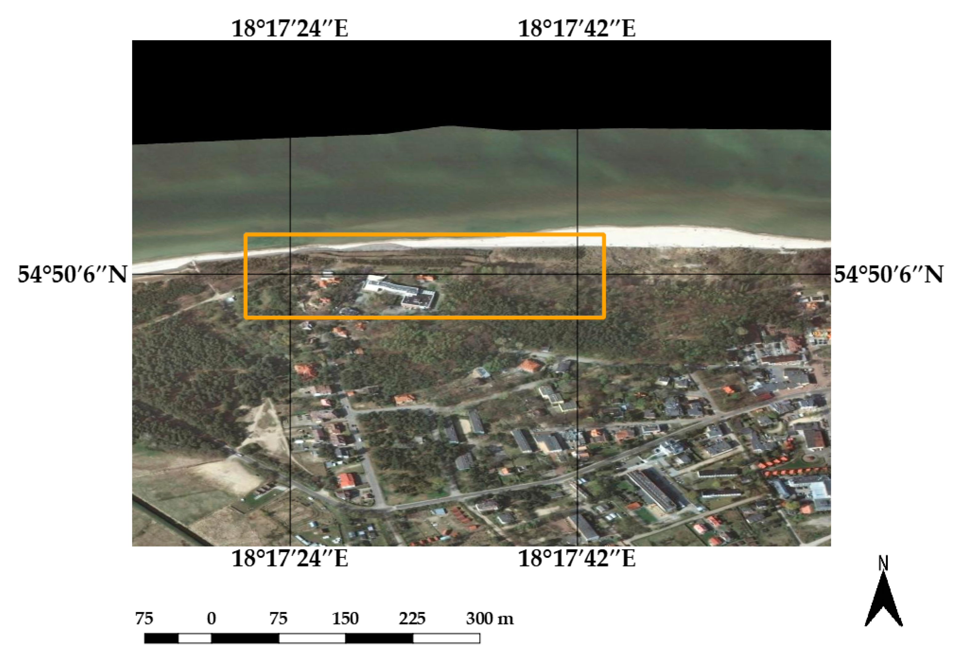
Jastrzebia Gora is located in the Gdansk coastal region, at the north-western end of the Kashubian Lakeland. Jastrzebia Gora includes the northernmost Polish location, which is marked with the “Star of the North” monument. The monument is located near the pedestrian promenade in an accessible location on the cliff and somewhat south from the most distant North point, which is located down on the beach. Figure 1 shows the location of the investigated section using an orthophotomap.
The investigated object is located in a section of shoreline that is hypsometrically between 133.8 km and 134.1 km. Its approximate coordinates are as follows:
- -
- latitude: 54°49′53′′N
- -
- longitude: 18°18′46′′E.
2.2. Environmental Conditions
Jastrzebia Gora is a region in which glacial uplands called clumps occur that are intersected by a series of valley forms that originate from archaic valleys from the Pomeranian and Vistula glacier periods. The upland height is 30 m above sea level in the vicinity of the shoreline.
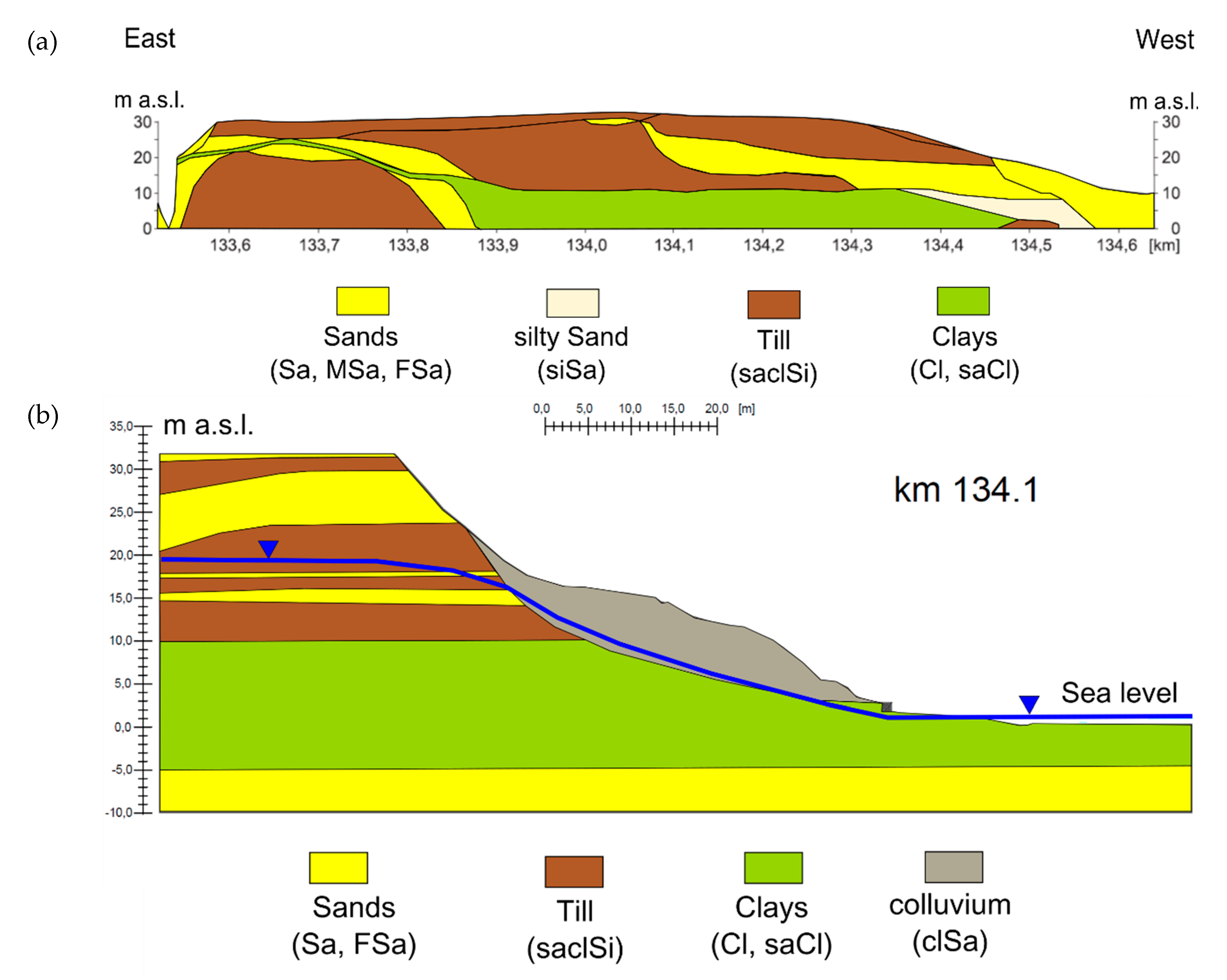
Abrasion has caused the cliff’s base to relocate due to sea activity; however, another landslide trigger is the geological structure. In the case of Jastrzebia Gora, an impact is made by a clay layer in the bottom part of the cliff. Drilling in the investigated area uncovered a clay stratum that reaches 10 m above sea level. The upper strata are made of different gravelly clays, sandy and silty clays, and medium and fine sands. The cliffs reach 30 m above sea level. In the sand stratum, there is a free groundwater mirror that can be detected on the slope’s side in the form of seepage [12,13].
The hydrogeological situation of the coastal Jastrzebia Gora zone comprises developed hydro-structural layers and a complex system of water circulation. Two water-conducting levels can, therefore, be distinguished: neogenic-paleogenic and quaternary with a tight hydraulic interconnection. One of the factors that can reduce the stability of a cliff coast is the flow of underground water. In the aeration region, there exist numerous levels of suspended water layers in a mosaic-like pattern, various filled chambers, and discontinuity triggered by glacial-tectonic disturbances. The rainfall permeability and inflow from the inland make the movement of the water periodic or continuous. These waters are partially under hydrostatic pressure. The permanent presence of water-carrying strata in the aeration zone leads to occasional plastification of surrounding tight clays. A significant threat is created by the water that fills the valley-like shapes in soils with low permeability. Here, the soil’s cohesion is mainly affected by the increased water content. Thus, slip surfaces emerge that result in landslides. Another threat to the stability of the cliff shore is the hydrostatic structure in the saturation zone. Slip surfaces that activate deep landslides are produced by plastic sediments just below the cliff base and below sea level. If the cohesion of these sediments is affected, an entire slope may lose its stability and a slip surface may occur that reaches under the cliff base and deep into the land on the cliff’s surroundings [12,13].
Figure 2a,b show longitudinal and transverse geological cross-sections of the cliff, respectively.
To summarize: The most important factors that affect the Jastrzebia Gora slope’s stability are:
- -
- a slow or rapid soil strata fall that follows the slope’s inclination (geological structure, terrain layout);
- -
- hydrogeological conditions: water outflow, pressure in different soil layers, and filtration;
- -
- rainfall; and
- -
- erosion due to the sea.
Note that complex hydrogeological conditions are an important factor that promotes the progressive movement of the soil mass, where soil particles are pushed by the water that flows from the cliff to the sea [15]. This issue is substantial in the case of colluvium propagation, as it creates difficulties with the reliable and realistic representation of a cliff’s geology and structure as an input for numerical modelling.
2.3. Measurement Methods
The present subsection describes the methods that were applied to acquire 3D data for further analyses. We used various laser scanning systems: Terrestrial, Mobile and Airborne. The airborne mission’s aim was to estimate the volumetric differences between models (created during each airborne mission). For the most sensitive (vulnerable) locations, i.e., those locations with the highest change in volume, measurements were made by means of a terrestrial scanner in order to precisely locate the highest variations. Table 1 presents the time schedule for the measurements.
2.3.1. Airborne Laser Scanning
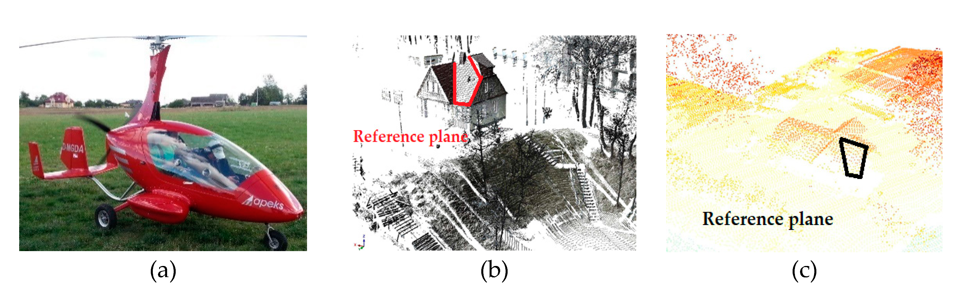
For airborne laser scanning, we used a Riegl VQ-580 laser scanner (Manufacturer: Riegl GmbH, Horn, Austria). According to the Riegl VQ-580′s specifications, the scanner’s precision and accuracy are equal to 25 mm. The measurement accuracy was assumed to be the same. In practice, the accuracy thresholds were found to differ, which was addressed in further work stages. The errors in the scanner’s position were complemented by the accuracy of the Inertial Measurement Unit/Global Navigation Satellite System (IMU/GNSS) system [20]. We designed and performed an experimental flight over the investigated area. Figure 3 shows the airborne system (a gyrocopter with a laser scanner attached to it), the reference planes that were registered with the help of the terrestrial laser-scanning system, and the same planes measured with the help of the airborne laser-scanning system. The designed flight lines along the coast were complemented by additional ones along the return route due to the low coverage between the flight rows. The air-scanning data were collected twice (in 2014 and in 2017). The missions aimed to obtain a sufficient point density (10 points/m2).
2.3.2. Terrestrial Laser Scanning
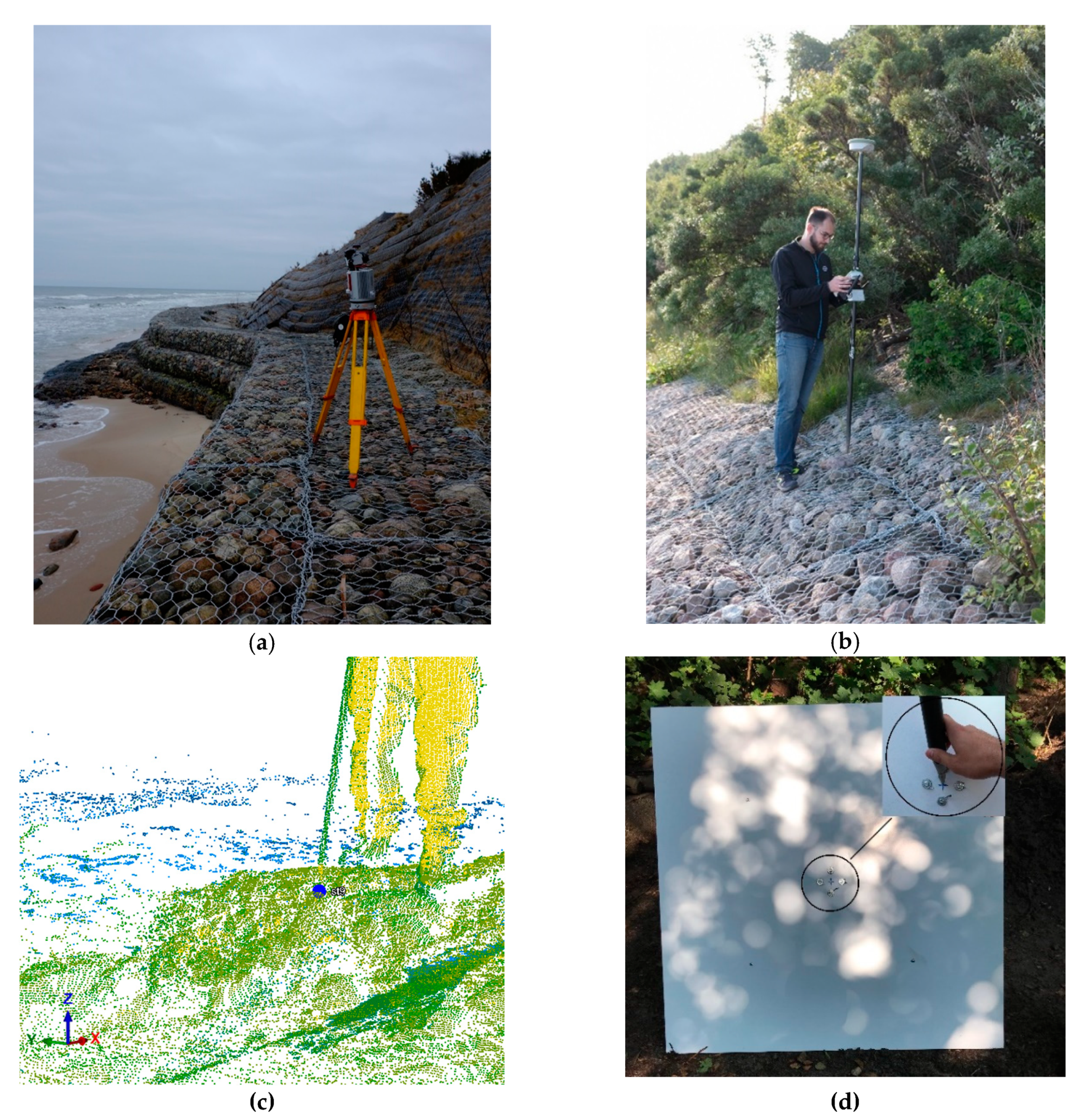
For terrestrial laser scanning, we used a Riegl VZ-400 laser scanner (Manufacturer: Riegl GmbH, Horn, Austria). This scanner allows for the remote acquisition of 3D data at high speed (122,000 pulses per second) and uses an infrared laser beam and a fast scanning mechanism. Compared to other instruments of this type, the Riegl device is a compact and lightweight measurement unit that can be installed in any orientation and does not require levelling. Note that the meteorological conditions, e.g., rain and snow, have a substantial impact on the device’s measurement quality [19]. Figure 4 shows photos of the scanner’s coverage of measurement courses in the Jastrzebia Gora region. The views are as follows: (a) a view of the scanner alone on the investigated object; (b) measurement of characteristic points using the GNSS technique in order to align 3D data that were referred to the EPSG:2177 coordinate system due to various measurement cycles; (c) the marked bottom of the pole on a point cloud, which represents a measured point in the EPSG:2177 coordinate system; (d) a materialized point that we deployed on an object of interest in order to unambiguously identify the reference points on scans. The size of this point is approximately 1 m × 1 m, and it has a sighting cross marked on the inside, on which we put a pole.
2.3.3. Additional Measurement Methods
We used data from the Riegl VMZ-400 mobile system (Manufacturer: Riegl GmbH, Horn, Austria) to analyse the airborne laser-scanning data. A description of the experiment that we performed at that time can be found in References [56,57]. The mission was served by a vessel with an immersion of 1.2 m, where the scanner was attached to a relevant structure in order to assemble the platform. The weather conditions at the time of the mission were advantageous (no rainfall, low air humidity, and a wind speed not exceeding Beaufort 4).
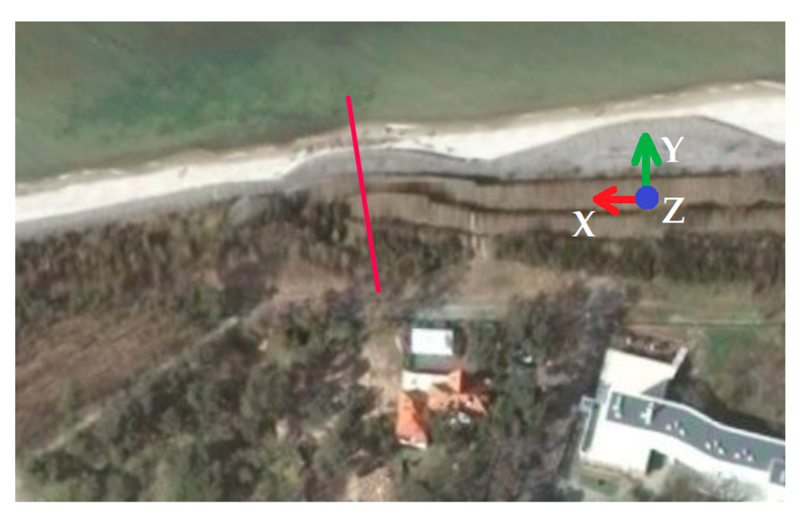
In order to study the exact pattern of a landslide’s behaviour and assess its threat to nearby infrastructure, we performed an experiment to measure the stabilized points at the top of the cliff under the hummus layer (Figure 5) in the local coordinate system. In this instance, we decided to change our assumption that the data were aligned with the EPSG:2177 coordinate system due to the fact that, locally, we were able to obtain greater accuracy. For this particular case, we used a Leica P30 Laser Scanner (Manufacturer: Leica Geosystems AG—Part of Hexagon). We used this instrument because it is possible to level it. This provided us with a simple orientation of the local system in such a way that the Y axis extended towards the sea, the Z axis extended upwards, and the X axis extended to the left according to the rule of the right hand. Figure 6 shows the location of the measurement points together with the orientation of the local coordinate system on an orthophotomap.
2.4. Data Processing
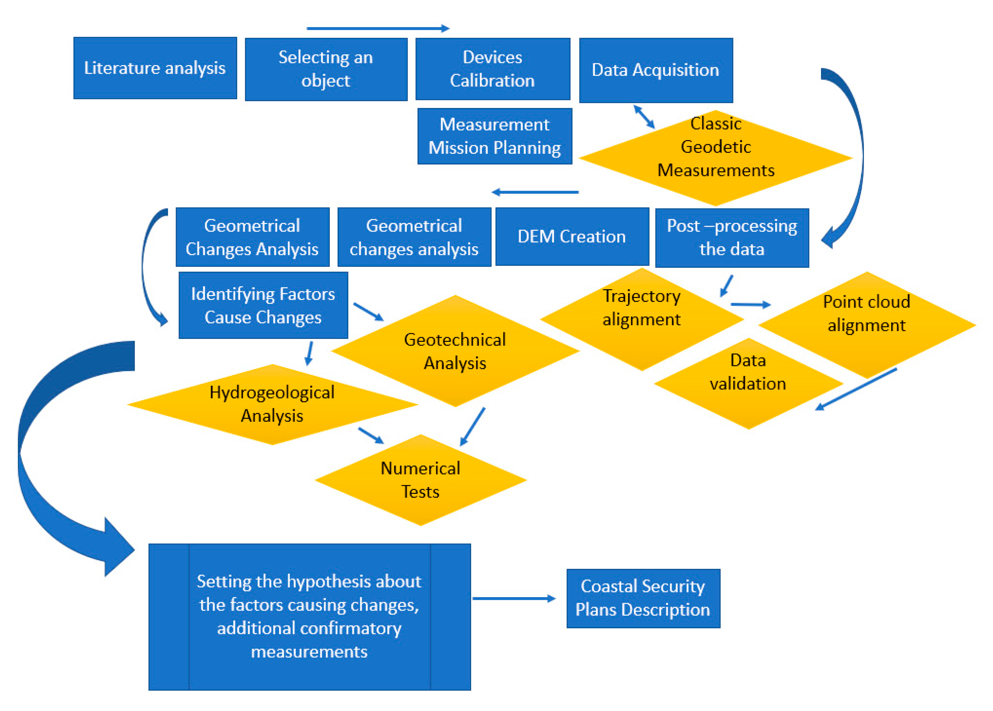
As shown in the scheme in Figure 7, we first performed a review of the state-of-the-art publications on the subject of coastal changes. Based on a prior study, we chose the investigation zone to carry out measurements and a computational solution for the accurate estimation of the displacement range and the origin. The measurement methods include classical surveying techniques that employ GNSS receivers and the Terrestrial, Mobile, and Airborne scanning systems.
2.4.1. Data Registration
In this subsection, we describe the ways to register data from terrestrial and airborne systems. Due to the fact that the mobile system was described in References [56,57], we do not focus on it here, particularly because, in our research, we used it to supplement the airborne system’s data from 2014. In describing our methods for particular experiments, it is very important to recreate them as well as the best possible assessment of the acquired results.
Terrestrial Laser Scanning
We focus on two aspects of the Terrestrial Laser Scanning data’s alignment. First, we present the methods we used to measure the cliff section. Second, we present the methods we used to establish the ground control network that was needed to properly align the data from the Airborne Scanning System.
After the scan positions were aligned, we obtained a solution for the appropriate cloud of points acquired from the airborne system and terrestrial system (the reference device) by applying the Iterative Closest Points (ICP) algorithm. It was considered to be successful due to the high coverage between scan positions and flight lines. The general working rule of the algorithm is based on an estimation of the translation and rotation of particular transformation elements (the principles of the algorithm are presented in Reference [58]). The basic version of the algorithm has three steps:
- -
- For each point in the reference dataset, find the closest point to the attached point by means of the closest neighborhood method;
- -
- assess the most relevant fit by means of the error matrix in the minimization process; and
- -
- transform the points to the new system in the attached set.
We used the Riscan PRO software (courtesy of ZUI Apeks Company Ltd.) to employ both the standard version of the ICP algorithm and a data-filtering method that segments the point cloud to identify the geometry of reference objects. The idea is the same as that presented in Reference [59], where a registration method uses a simple geometric after extracting it from scanned scenes. A description of the workflow can be found in Reference [60]; however, we recommend reading the RiScan PRO Manual.
In the second step, we aligned the obtained point cloud to the EPSG:2177 coordinate system by means of a GNSS receiver operating in Real Time Network (RTN) mode (in our research, we used a TOPCON Hiper V receiver (Manufacturer: TOPCON Corporation, Tokio, Japan) and a Leica 1200 receiver (Manufacturer: Leica Geosystems AG—Part of Hexagon)). These measurements involve the use of several reference stations to calculate corrections. The measurements were made in such a way that at least four control points were visible from each station. After receiving the approximate position of our GNSS receiver via an NMEA GGA message, the computing system created a virtual reference station near the receiver and calculated the corrections for it, which were sent as if they came from a single reference station. To perform calculations, the computing system collected and interpolated patches from several user-facing physical reference stations. The accuracy of the measurements was the same as when using the Real Time Kinematic (RTK) method [61,62]. After the measurements were made, the transformation of the data from the local coordinate system to the global coordinate system took place through a transformation using the system’s rotation and translation. In order to acquire proper results, we used a standard rotation–translation matrix where to interpret the elements of spatial rotation we used simple trigonometric functions of the rotations about the three axes of a cardan system. On the other hand, the standard deviation, which was calculated as a statistical test to check the fit quality, is presented in Equation (1) as σ1.
where N is the number of points, and D is the difference in distance between the local and transformed coordinate systems. The results, in the form of the value of deviation, are given in Section 2.4.1.
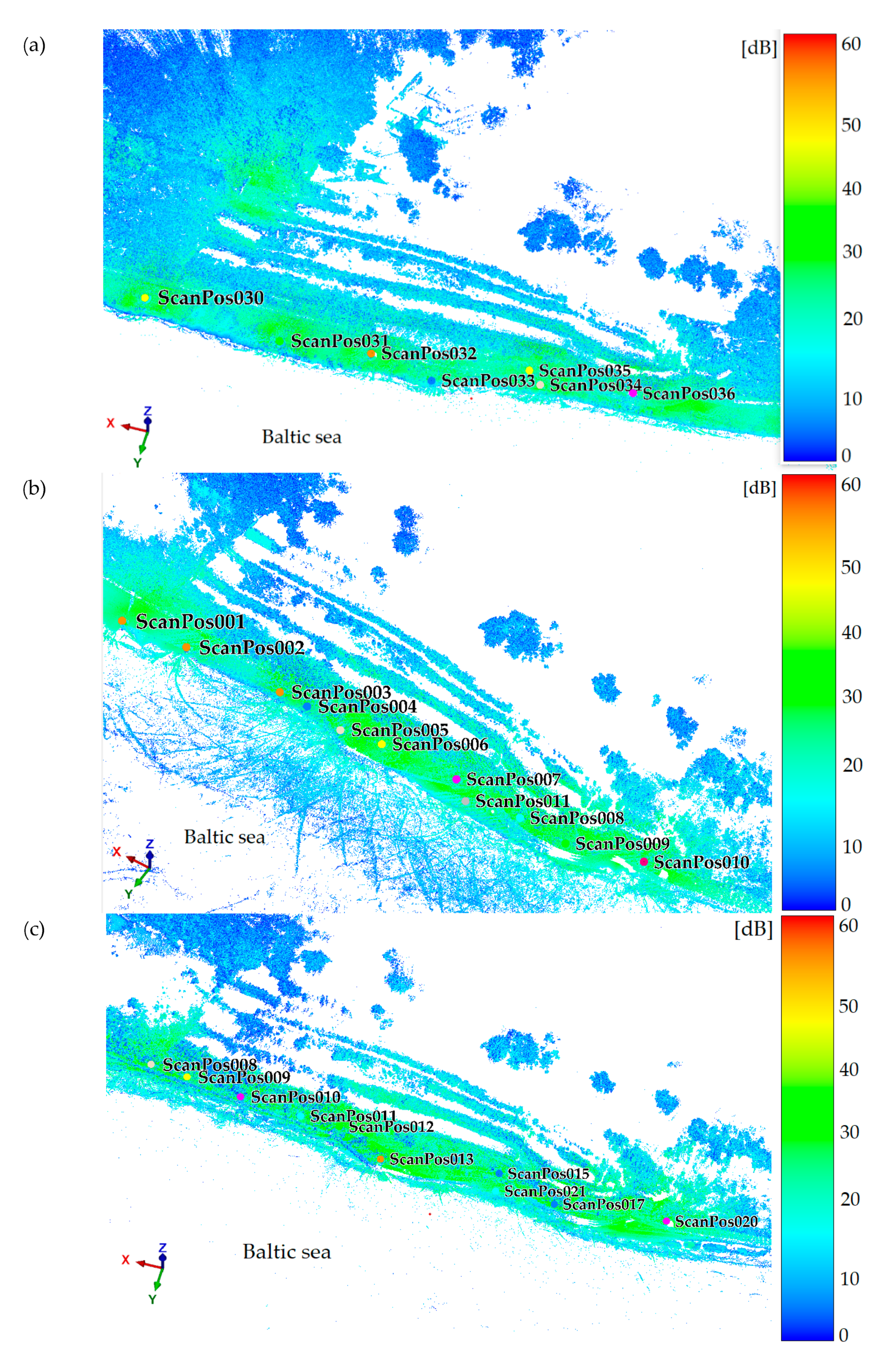
Figure 8 presents the location of the scan positions for each of the February 2015, March 2017, and July 2017 measurement missions and the deployment of positions in the local system in November 2017 and March 2018. The point density for each measurement mission was equal 4200 pts/m2. In Figure 8a–c,e respectively, colours are presented as a function of light reflection amplitude, while Figure 8d shows the fragment of the upper part of the cliff in RGB (Red-Green-Blue) colours.
Airborne Laser Scanning
To process the Airborne Laser-Scanning data, we first covered the trajectory alignment from the Inertial Navigation System (INS) system (the INS system consists of a GNSS receiver and an IMU unit) using the Aerooffice and Grafnav software (courtesy of Apeks Ltd.), and then manually implemented the control objects to align the scans with each other using the ICP algorithm in the RiProcess software (courtesy of ZUI Apeks).
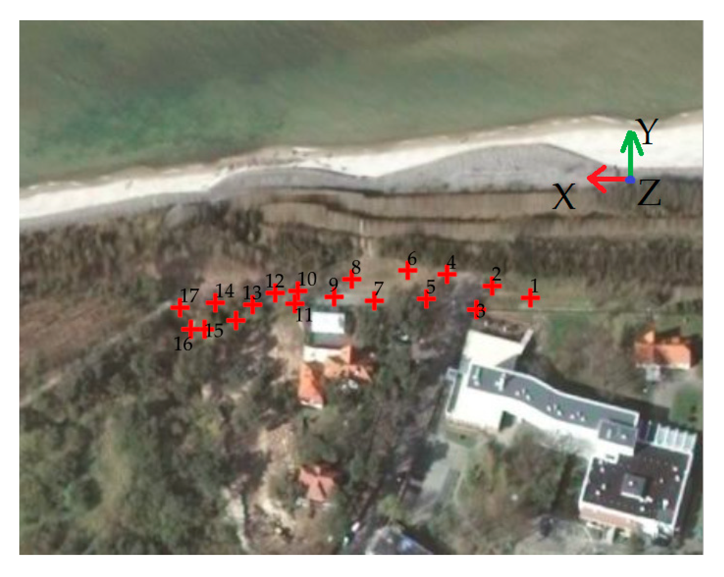
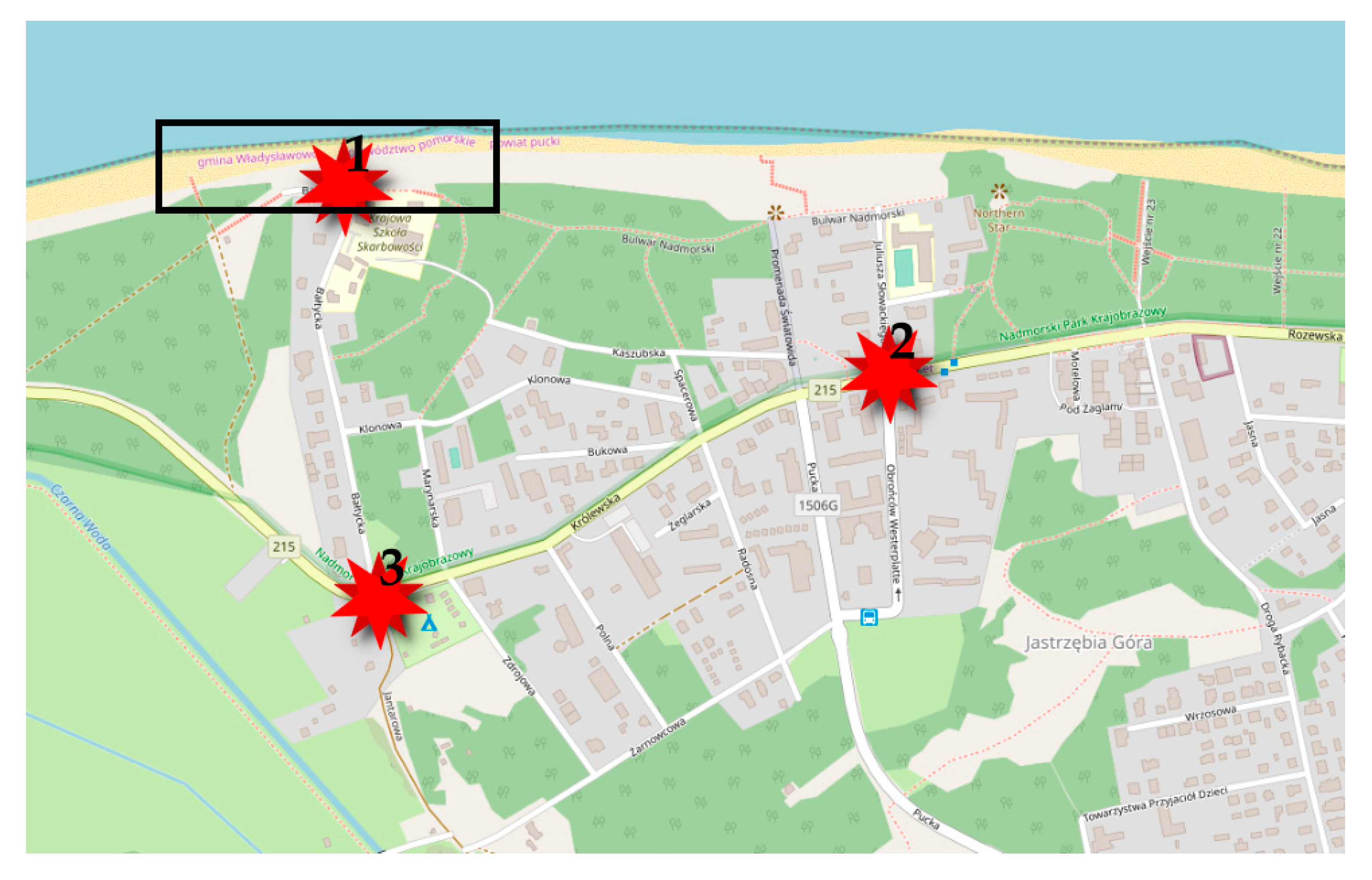
To measure the control points that are necessary for a proper data alignment with the EPSG:2177 coordinate system, we used a GNSS Topcon HyperV receiver (Manufacturer: Topcon Corporation, Tokyo, Japan) and a Riegl VZ-400 laser scanner (Manufacturer: Riegl Gmbh, Horn, Austria). The idea was to place the laser scanner near the characteristic points, e.g., roofs of buildings, acquire data from one scan position, and then align them with the EPSG:2177 coordinate system based on the previously measured points by a GNSS technique. In each case, the measurement required us to establish a minimum of four points. Figure 9 shows the location of objects we measured (using the OpenStreetMap map) in close proximity to our area of interest.
To align the trajectory, we needed to adopt proper rules in order to carry out a proper flight. First, we had to ensure a static initialization of the INS system. Next, we had to be sure that the entire measurement mission would be covered by the reference station (we used the VRS (Virtual Reference Station) for this purpose) and that the airborne system would fly in straight lines. A description of the trajectory alignment method can be found in the instruction manuals of the GrafNAV and Aeroofice programs.
2.4.2. Data Filtering
In order to obtain information on terrain, the filtering of laser scanning data into terrain and off-terrain points is essential. We divided our data filtration process into three stages:
- -
- In the first stage, we reduced the number of points by removing those points from the dataset that were characterized by a deviation associated with the intensity of reflection (i.e., noise);
- -
- in the second stage, we separated the outliers from the dataset using a height filter;
- -
- in the third stage, we calculated the numerical surface from the remaining points and, in the hierarchical process, we removed outliers from the dataset to eventually obtain points that only represented ground truths.
In the last stage, we used the interpolation method for the movable polynomial of the second order. This means that its parameters are approximated on the basis of data from the local neighbourhood of the point. Due to the point density, we used the approximation by the least squares method of this polynomial in the defined areas where the product of neighbourhood weights and height deviations in these points must converge to the minimum (2):
where pi is the weight of the neighbourhoods, and vi is the deviation of the heights at the neighbourhood points. The vector of unknown polynomial equations can be calculated using Equation (3):
where matrix X is the matrix of polynomial coefficients; matrix A is the matrix of coefficients x and y; matrix P denotes the observation weight matrix; and matrix H denotes the height of the corresponding points x and y. It is very important that, in the first process, each point has exactly the same weight. Only after an approximation of the surface and obtaining the distance of points from this surface, can we filter the set of points from the outliers. We then carried out the filtration process again. During the last stage, when the distances from the surface did not differ significantly, the remaining points that did not belong to the soil class (noise) were removed manually.
The idea for data filtration was taken from Reference [63], where Jozkow presents the most effective methods for processing laser-scanning data. For the analysis of the cross-section that is described in Section 3.1, we used raw clouds that were only aligned with each other. Filtration and modelling were implemented for the airborne laser-scanning data.
2.4.3. Digital Elevation Model (DEM) Creation
To develop the numerical model in the form of a TIN grid, we used the Delaunay 2.5 D triangulation method. Triangulation was performed only for the 2014 and 2017 airborne missions in order to calculate the volume shown in Section 3. We decided to use this method as it uses all points from the dataset. It gave us confidence that the closed surfaces of the model would not distort the results on the obtained volume.
To carry out the triangulation, we used the reference plane, which we called the “0” plane. It was fitted to a set of points located on the beach, close to the shoreline, where the height differences are not significant.
Based on the assumptions that are described in the introduction, in which the data model in the form of a TIN grid is used to determine the location of the largest displacement, we decided to evaluate the accuracy of the calculated volumes (described in Section 3.1) in terms of the quotient between the measured volume and the increase in the volume by 3σ1 calculated residuals from the reference point clouds. We express this value as a percentage. The point density for the flight data acquired in 2014 equals 12 pts/m2 and 13 pts/m2 for year 2017.
2.5. Data Validation
The results section describes the quality and validation of the obtained 3D data.
2.5.1. Terrestrial Laser Scanning
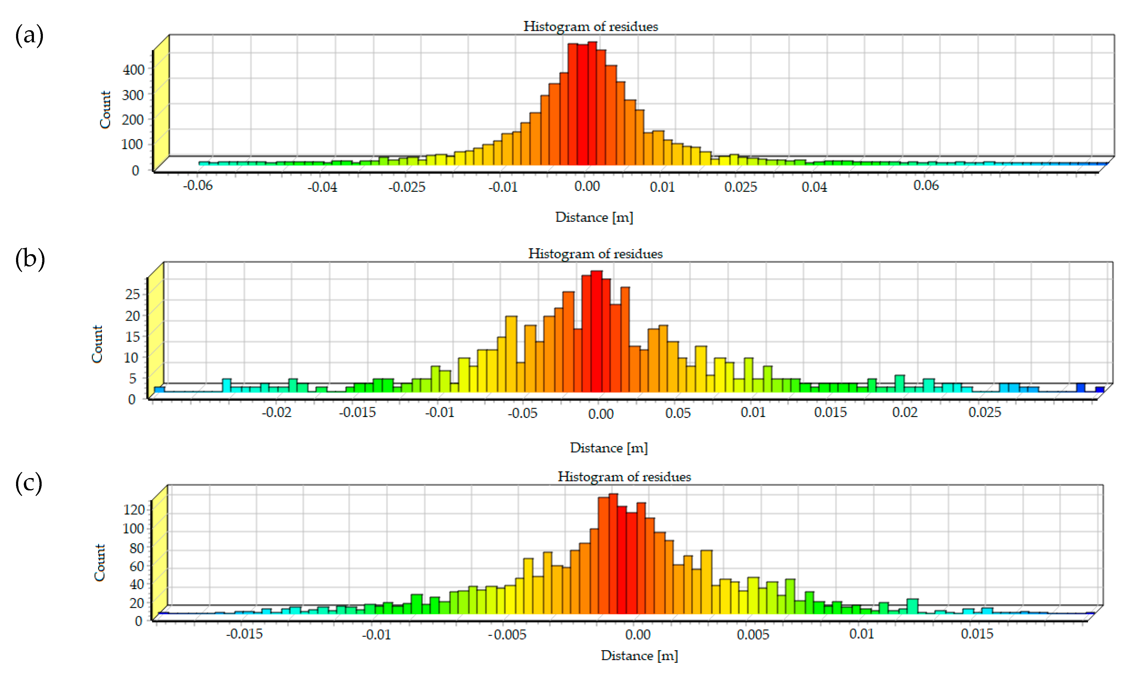
The validation of the terrestrial laser scanning data was based on a histogram of the distance between the control points. We applied the ICP algorithm (Figure 10) and the standard deviation and attached a point cloud to the EPSG:2177 coordinate system (Table 2). We needed to provide a fixed GNSS receiver solution where the error in the calculation of the average position would be no more than 1 cm. In the case of an erroneous measurement by satellite technology, the standard deviation of such an aligned point cloud to the EPSG:2177 coordinate system would be a decimetre, or even higher, and thus easy to detect. Based on the obtained results from Figure 10 and Table 2, we assumed that the accuracy of the comparative analyses may fluctuate around 10 cm (2.5 σ1) when using Terrestrial Laser Scanning. For this reason, the precision of the displacement reading will also be in the range of 10 cm. Table 2 presents the transformation matrix in the first column, number of reference points used in alignment process in the second, and the value of the calculated standard deviation in the third. The presented residues show the differences in distance between the tie points in the case of automatic extraction described in Section 2.4.1.
2.5.2. Airborne Laser Scanning
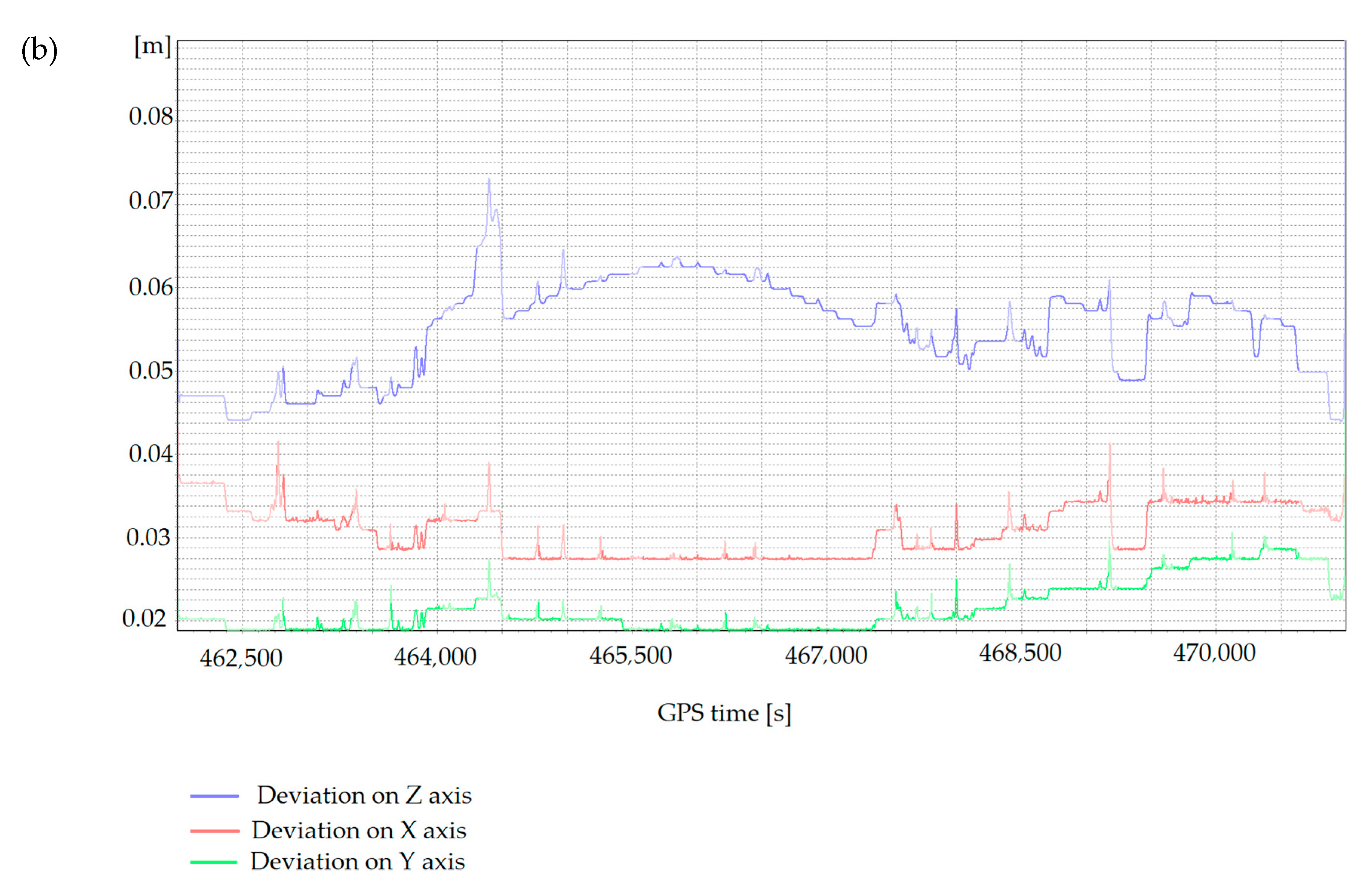
Furthermore, analyses of the airborne system’s data were conducted. Figure 11 shows a diagram of the INS position deviation based on trajectory, and Table 3 shows a histogram of differences among control points. As can be noticed in Figure 11a, which shows the deviation from the flight that was performed in 2014, the elevation has the highest value of deviation of 6 cm. Figure 11b, which shows the deviation from the flight that was performed in 2017, has similar values to those in Figure 11a. This means that the trajectory was correctly aligned. An assessment of the accuracy was carried out after establishing individual records of scans between them and the EPSG:2177 coordinate system. The resulting differences between the accuracy of alignment of individual axes result primarily from the measurement characteristics, where the aircraft fluctuated, but also from the emerging drift of the device. Seen offsets can be removed during strip-adjustment procedures.
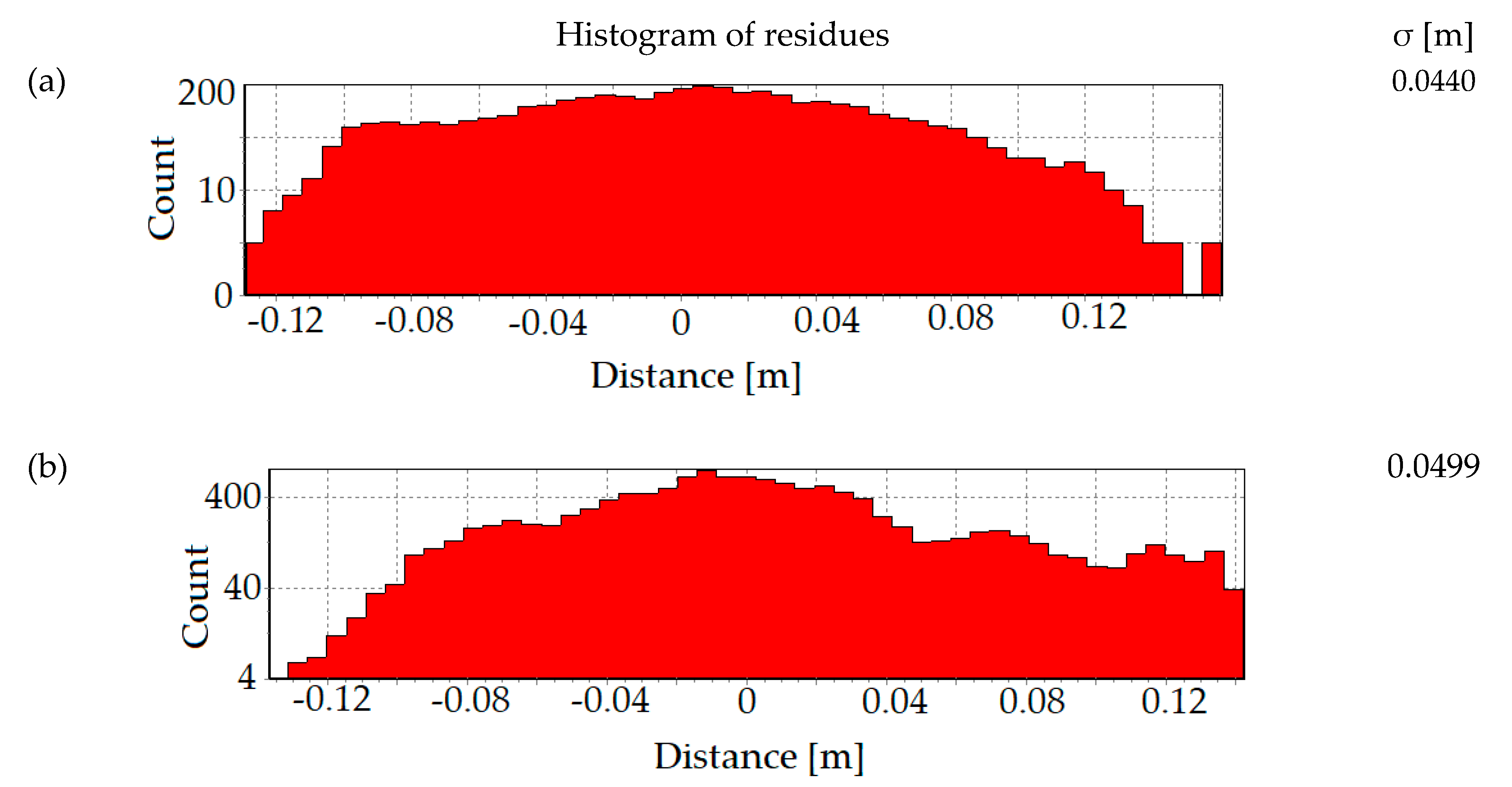
Based on the results obtained from the alignment of laser strips with each other as shown in Figure 12, the standard deviation values for these values (for the 2014 flight, σ = 0.044 m; for the 2017 flight, σ = 0.0499 m) and the irregularities that are visible in the trajectory shown in Figure 11, we assumed that the accuracy of one model varied at the level of 3σ, which is 0.132 m for the flight from 2014 and 0.149 m for the flight from 2017. These values mean that the summed accuracy of the comparative model will be in the range of 20–30 cm. The presented residues show the differences in distance between the tie points measured by surveying methods and in the case of automatic extraction described in Section 2.4.1.
2.5.3. Additional Measurement Methods
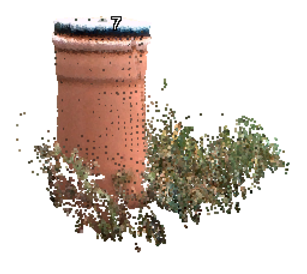
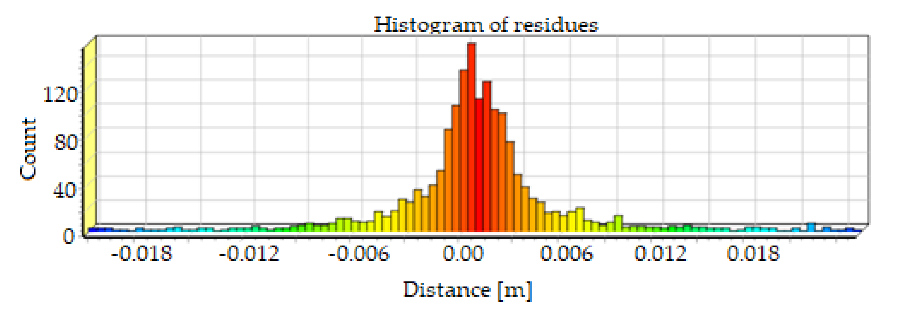
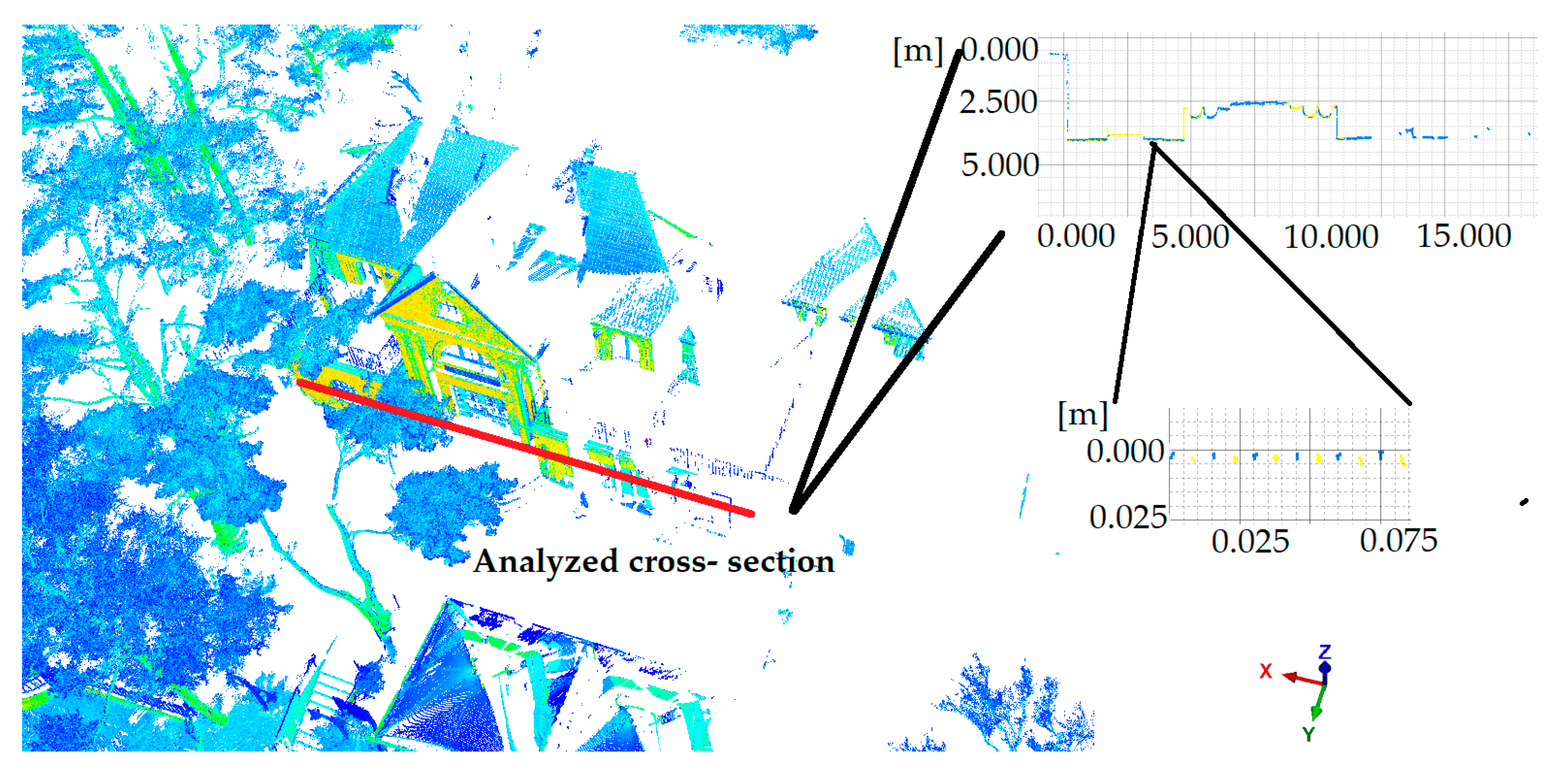
We analysed the accuracy of the measured points in the form of sewer pipes that were located at the top of the cliff. We wanted to achieve greater accuracy (at the level of 1 cm) to check our assumptions about the landslide’s origin and to verify whether there is a threat of a landslide being initiated (the elevation should decrease locally in this case). First, we analysed a histogram of the distance among control points and then checked the quality of the alignment by creating cross-sections through buildings that the landslide did not have an impact on (in theory, they should be located in exactly the same place). Figure 13 shows the histogram of the distance among control points. Figure 14 shows the analysed building cross-sections.
Based on the results, we assumed that the accuracy of the displacement readings of points in the local system is about 5 mm. We selected this value predominantly due to noises that were recorded on terrain obstacles that are actually flat.
2.6. Stability Analysis Methods
Calculations of a slope’s stability fall within the ambit of geotechnical engineering. A commonly used measure of stability is the so-called Factor of Safety (FS) parameter, which indicates a safe state (FS > 1) or a progressing failure (FS < 1). The larger the margin is over unity, the better; with respect to earth constructions, it is recommended that safe slopes be regarded as having an FS > 1.25 or even 1.50, depending on importance (e.g., higher values are recommended for earth dams). This is caused by uncertainty in the geotechnical parameters, which are measured at selected points only (boreholes).
The stability of a slope is a function of two factors (or groups of factors): geological structure (geological layers, geotechnical parameters, water levels and flow) and geometry (inclination). For given geological conditions, the only variable that has an influence on stability is the cliff’s geometry. In order to assess the conditions that need to be satisfied to trigger a landslide, we first decided to estimate the stability using the limit equilibrium method [50,51]. The chosen cliff cross-section was modeled using an elasto-plastic model with the classical Mohr-Coulomb yield criterion. The Factor of Safety (FS) for Mohr-Coulomb material with the Shear Strength Reduction (SSR) method [64,65] was calculated using Equation (4):
where the strength parameters φ’—effective angle of internal friction and c’—effective cohesion are the measured ones, and those indexed with ‘m’ are the reduced ones in a state of failure. Table 3 shows the geotechnical parameters that we used for the numerical calculations. The values are based on Reference [10].
γunsat and γsat are the volumetric weight of the soil (in natural moisture content) and the saturated soil, respectively. E0, soil deformation modulus; ν, Poisson’s ratio.
We also performed probabilistic sensitivity analyses to assess the impact of soil parameters on the computational results. In order to do so, we analysed interactions between selected variables and the safety coefficient using the Monte Carlo algorithm. We defined the reliability index as:
where RI is the Reliability Index, FS is the Factor of Safety due to a population of n Monte Carlo runs, and is the standard deviation of the FS due to n Monte Carlo runs.
The project’s capacity and the amount of collected 3D data mean that it aims to develop a methodology for monitoring cliff shore slopes that can be successfully applied to identify threats of landslides, estimate their magnitudes, and propose methods to prevent failure mechanisms from progressing in order to improve a shoreline’s safety.
3. Results
3.1. Interpretation of Measurements
Figure 15 shows the terrain model that was created as a result of the measurements in the form of a triangulated point cloud for the airborne system’s data that were acquired in 2017.
The geometric analysis features a volume comparison between the 2014 and 2017 models computed from the airborne scanning system’s data. The main concern is understanding the geometric changes in the cliff. To calculate the volume, we created a plane on the zero level in the EPSG:2177 coordinate system (as described in Section 2.3.3). In order to identify the highest deformations, we compared the 2014 and 2017 models; Figure 16 shows the results. Based on the comparison, we found the location of the most significant change in the cliff’s geometry. First, we defined a 10 m × 10 m grid in the investigated area to perform a more detailed analysis. Figure 17 shows: (a) the location of the analysed area; and (b) the defined 10 m × 10 m grid. Each grid square was used to compute the volume in order to choose a section to analyse (the geotechnical stability analysis). Figure 18 shows the resulting sub-quantity volumes. In addition, Table 4 present the percentage error in the calculation of this volume (as described in Section 2.3.3). The computation of this error consisted in calculating the quotient between the determined volume, and the volume increased by 3σ separately for the data from 2014 and 2017 (the 3σ for the flight from 2014 is 0.132 m, and the 3σ for the flight from 2017 is 0.149 m). The detailed description of obtaining the σ value is described in Chapter 2, respectively, in Section 2.4 and Section 2.5. The idea of showing the percentage error in volume calculation was obtained from Reference [66] where, according to standards, the numerical modelling method can be used to calculate the volume of masses, while the relative error in the volume calculation should not exceed: (a) 6% of the volume for between 0 and 20,000 m3, (b) 5% by volume for between 20,000 and 50,000 m3, (c) 4% by volume for between 50,000 and 200,000 m3, (d) 3% by volume for between 200,000 and 500,000 m3, and (e) 2% by volume for the range over 500,000 m3. Therefore, the relevant rows A and partially B from Table 4 and Table 5 should not be taken into account in the analysis of changes in the volume of earth masses, however, due to the very small volume values in these rows, this does not affect the estimation of the overall mass flow down the slope.
As can be observed in Table 4 and Table 5, the largest percent error values are in places where the volume values are the smallest. In places with the largest volume changes, the error rate is 1–2%. In these places, even increasing the standard deviation to 6σ in the error calculation formula will not change the accuracy significantly. This means that the differences we calculated are adequate for the analysis above a certain level. We set this level at a distance of 20 meters from the shoreline, i.e., where the error percentage is minimal and has a value of 1–2%. To assess the accuracy of the comparison presented in Figure 16, we assumed the worst case scenario, in which the calculated error from the two flights is summed.
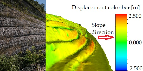
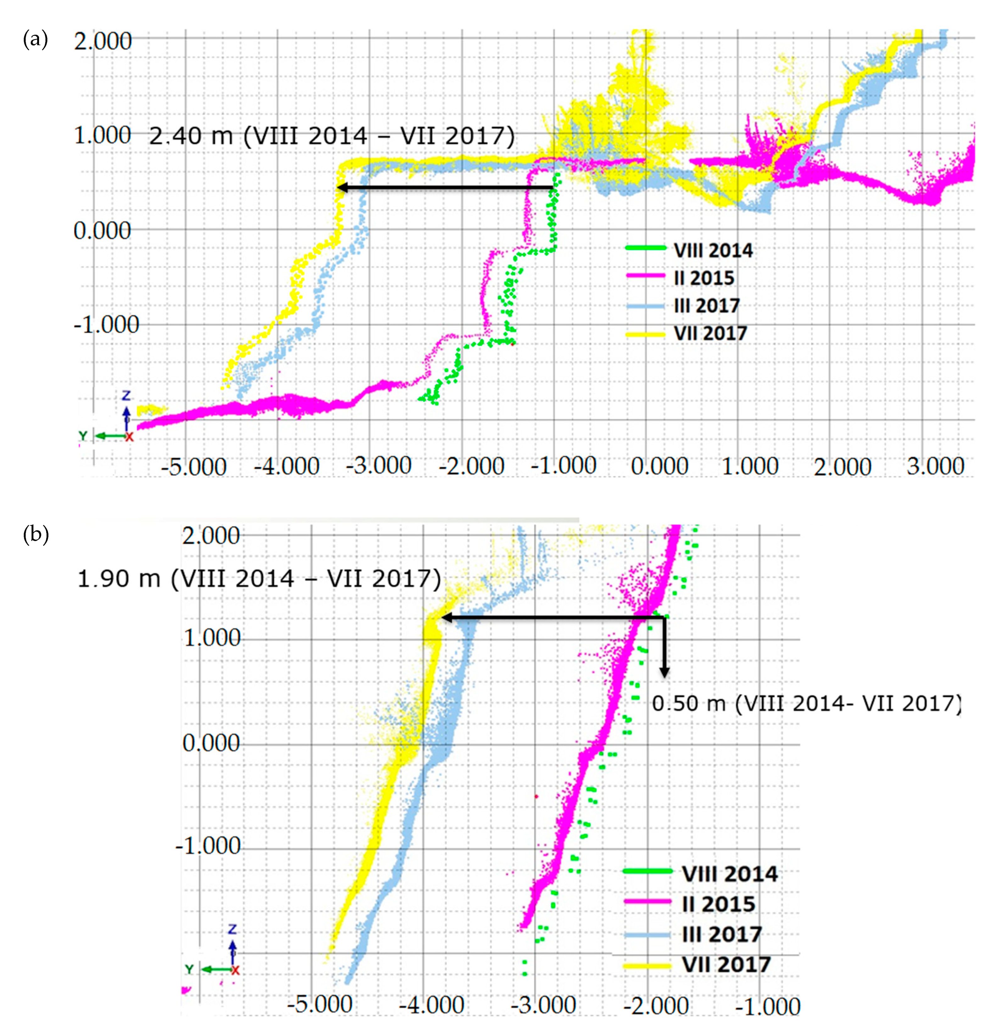
Based on the volumetric results, we chose for further investigation a section between the mesh columns marked C and D. The deviations in the same section (as shown in Figure 19) that were obtained from a geometric analysis of the gabion structure and the reinforced soil are shown in Figure 20a,b, respectively. We marked the month and year of the measurement and linked them to relevant colours.
It can be observed that the gabion reinforcement’s movement was horizontal (Figure 20a), and the value of the soil’s movement reached 2.4 m over 3 years. This is a substantial deformation of the cliff’s base, which has an influence on its higher parts. Another part of the cliff, which is constructed from soil reinforced with geosynthetics (Figure 20b), showed a smaller displacement (1.9 m) in the direction of the sea, but also displayed a substantial settlement (vertical displacement) of about 0.5 m over 3 years.
3.2. The Results of the Cliff Stability Analysis
Finally, we performed geotechnical computations in order to identify the factors that most affect the slope’s stability. If the factors are known, it is possible to properly formulate plans for the shoreline’s preservation. The computations were performed under actual hydrological conditions as well as with an elevated groundwater level (produced by, e.g., high-volume rainfall or an increase in sea level during a storm). We used two limit equilibrium methods (the Morgenstern-Price (M-P) method and the Spencer method) as well as Finite Element Method (FEM) simulations [67]. The results, which are presented in Table 6, show that, under actual conditions with no sea level rise, two possible variants (elevations of +0.8 m and +0.9 m in the water table) and one of a very low probability (+ 8.0 m) can achieve a Factor of Safety that is close to/lower than 1.0.
Computed results shows very similar values of Factor of Safety for both limit equilibrium methods while showing lower ones for Finite Element Method in same conditions. We see that for actual groundwater level and real-life level rise (+0.8 m and +0.9 m), Factor of Safety does not decrease significantly, so there is no major influence of groundwater on stability (assuming other factors constant). The influence of water level we can observe after rising it much more (+ 8.0m), which is quite unrealistic (but possible: e.g., heavy rainfall & water supply pipe breakage). Table 7 presents an additional statistical parameters assessment, namely Probability of Failure (PoF) and Reliability Index (RI) values calculated for the above scenario of water table elevation, using Monte Carlo simulations [48]. Here we can observe very similar values of FS, as for limit equilibrium methods. Additionally, one can note low risk measures (PoF and RI) in three real-life cases (0.0 m, +0.8 m, +0.9 m) and substantial risk in the last one (+ 8.0 m).
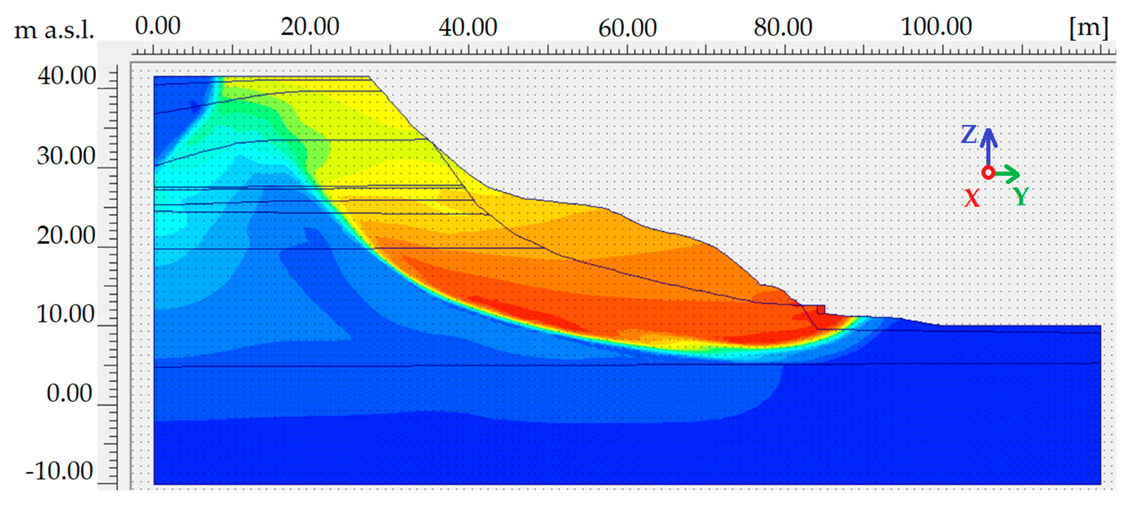
To evaluate the influence of the input data’s quality on the calculations of stability, a classical sensitivity analysis was also performed with respect to the different soil layer parameters. This is an important issue in three geotechnical respects: (1) the uncertainty in the values from archival investigations [11,48] (c.f. the authors in Reference [65] used slightly different parameters that were obtained from another source); (2) the complicated geology and possible variability in the parameters in the soil profile; and (3) the fact that water can change the values of soil parameters (e.g., it can lower cohesion). The analysis showed that, for the initial case (no elevation in the water table), the most sensitive parameters were the friction angle and the cohesion in the bottom layer (the clay from which the cliff is built). This is logical, as this scenario triggers a path that leads to the cliff’s destruction (see Figure 21).
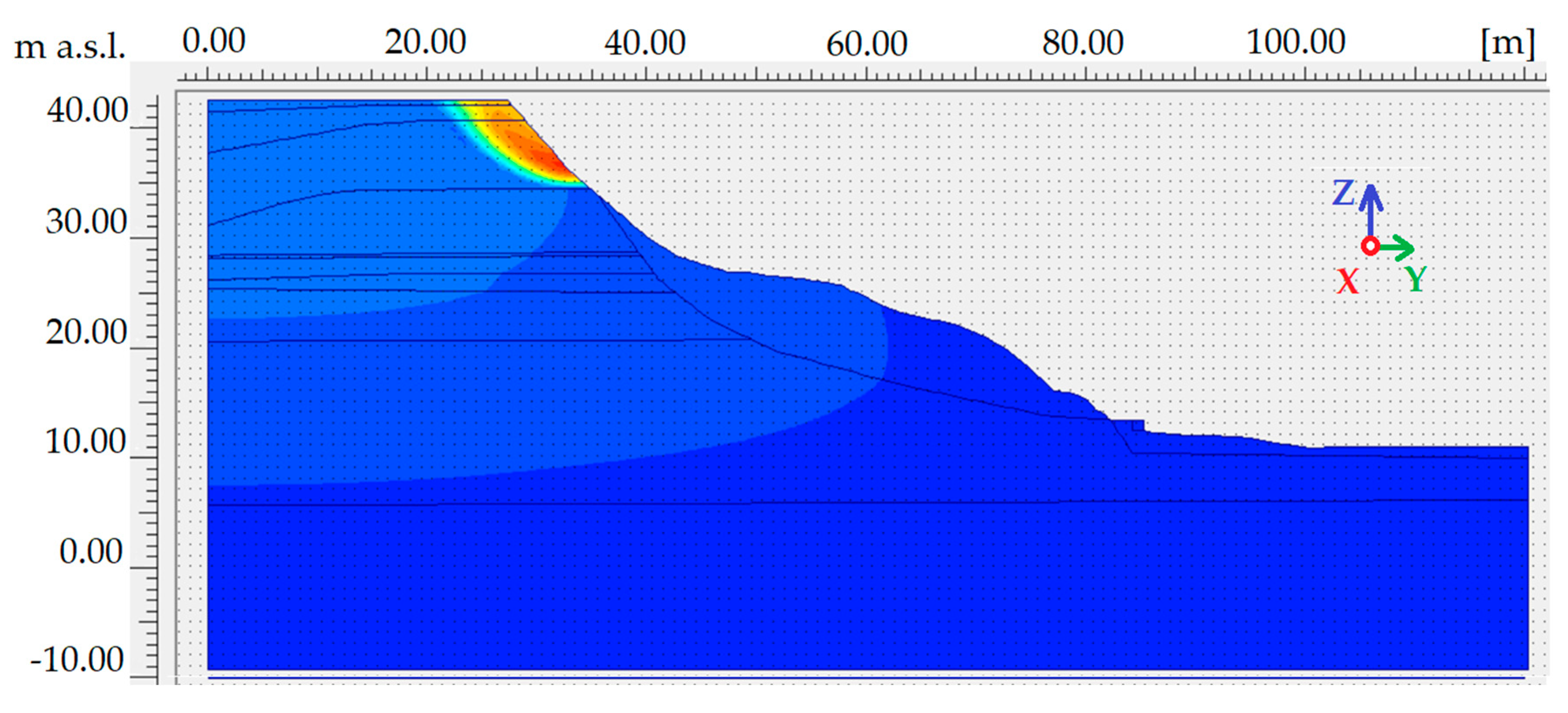
It is worth emphasizing that the cohesion is not constant for a given soil—it reduces with increasing water content. In complicated geological conditions, even a thin layer of sand interbedding the clays can deliver a substantial amount of water into the clay layer and reduce cohesion. It is also interesting to note, that slight water table elevation from +0.8 m to +0.9 m causes failure path transformation from a global (Figure 21) to local one (Figure 22). In this case, the most sensitive parameters are the cohesions of both layers building local slip surface: till and clayley sand, followed by friction angle of both layers. The resulting interpretation is similar to the previous case: The change of geotechnical parameters caused e.g., by a substantial water content increase, can result in a sudden landslide.
3.3. Additional Measurements
In order to verify the soil deformation pattern with higher precision, additional measurements were made using a terrestrial laser-scanning system in the local coordinate system of points below the lower hummus layer, which was represented by a plumbing installation (described in Section 2.3.3). Table 8 presents the displacement in the points. The measurements were made at the end of November 2017 and in March 2018.
Based on the local coordinate system that served for the measurement, its accuracy was estimated to be 5 mm (Section 2.4.3). Due to the horizontal displacements, no significant differences were detected; however, in the case of the vertical displacements, we detected differences with values in the centimetre range. These may cause cracks to be made in the soil that allow for a more intensive infiltration of freezing water into the cliff’s body. This tendency needs to be verified in the coming years. The measurements indicate that there was no local decrease in the elevation in the area of study, which suggests that the landslide temporarily did not include the cliff’s crown. On the other hand, the occurrence of a landslide could happen at any time, so regular monitoring has to be performed. These results also confirm the need to plan and execute additional geotechnical and hydrogeological investigations in the area.
4. Discussion
Based on differential maps and volumetric analyses, the most deformed part of the Jastrzebia Gora cliff was identified. The analyses were undertaken twice in 2014, once in 2015, and twice in 2017. The maximum deformation (2.5 m) was detected between two extreme measurements. The working assumption that we made at the start of the analysis stated that the cliff would move continually and proportionally towards the sea until the gabions and the reinforced subsoil were broken. Our analyses showed that in 2014–2015 the cliff moved approximately 30 cm, and in 2017 the cliff moved approximately 50 cm; thus, the movement is not consistent. A detailed image of the cliff’s geometry allows us to analyse it numerically in order to assess its stability. Additionally, the use of laser-scanning technology to monitor the cliff’s surface allows us to detect very small amounts of soil deformation, as described in Section 3.3. A hypothesis may be put forward that the soil elevation was caused by the freezing of water below the soil stratum. Thus, in future work, further monitoring of this zone will be conducted.
We also performed geotechnical stability analyses. Using archival data on soil parameters, the cliff’s initial stability was determined. The Factor of Safety for the cliff in its initial state was calculated as FS = 1.293. Hence, the cliff in its initial state can be considered to be safe (depending on the adopted margin of safety; e.g., some guidelines state that safe slopes have an FS > 1.25, while others state that safe slopes have an FS > 1.3 or even 1.5). The next step in the numerical simulations assumed an elevation in the groundwater level in order to check how this affecfcliff’s stability. In the case of the investigated section, an elevation in groundwater level was found to not affect the cliff’s stability very much. However, it was observed that the failure path transformed from global to local due to a slight rise in the groundwater level (the change occurred when the level was between +0.8 and +0.9 m).
A substantial amount of information on the cliff’s performance was obtained by a sensitivity analysis based on the cliff’s initial state and including all soil parameters in the investigated section. The results showed that a change in selected parameters may strongly affect the cliff’s stability or even lead to a landslide. The results also showed that the sensitivity of different soil layer parameters depends on the level of the groundwater level. In the global failure path case, i.e., the actual groundwater level, a loss of stability may be caused by a change in the cohesion of the clay layer (the bottom part of the cliff). When a loss of local stability was detected, where the elevation in the groundwater level exceeded +0.9 m, the most sensitive parameters changed to those belonging to local slip soils. These results provide an indication of just how complex the stability of the Jastrzebia Gora cliff may be, how many factors affect it, and the possible range of a landslide (regarding both local and global stability).
5. Conclusions
The analysis showed that, while stability factors of the cliff’s present state (assuming the presented soil layers and their geotechnical parameters) were marginally greater than 1.0, many other factors had an influence on the cliff’s stability. Thus, we observed displacement of reinforced soils and gabions despite the fact that they were primarily constructed to prevent the cliff from degrading and to protect the infrastructure—we may call this state a ‘creeping loss of stability’. To overcome this problem, a detailed soil structure investigation is required.
To summarize, a coherent methodology may be proposed to monitor sea cliffs. First, a reconnaissance flight is needed that applies an airborne scanning system (carrying out a mission using a drone may also be effective [68]) to identify the location of the highest variation on the basis of differences in the distance between two models (from different missions in time). Then, an analysis of changes in geometry is to be conducted by more accurate methods, e.g., terrestrial laser scanning. An understanding of changes in geometry allows us to identify the most-threatened sections that require a geotechnical investigation (a field investigation to determine the actual soil parameters and make hydrogeological measurements), followed by a numerical analysis, in order to identify the factors that trigger a loss of stability. Additional measurements will allow us to assess the variation in the characteristics of sea cliffs and to take the necessary steps to improve the shoreline’s safety.
Author Contributions
Data curation, P.T.; Formal analysis, P.T.; Investigation, M.P. and R.O.; Methodology, R.O. and P.T.; Project administration, P.T.; Resources, P.T.; Supervision, M.P. and R.O.; Validation, M.P. and R.O.; Visualization, P.T.; Writing—original draft, R.O. and P.T.; Writing—review & editing, M.P., R.O. and P.T.
Funding
This research received no external funding.
Acknowledgments
The authors express their gratitude to the Apeks Company for the equipment and software that were used in the data acquisition and post-processing. The mobile laser-scanning data were obtained from a project that is part of an operation by the Intelligent Development Operational Program for 2014–2020 Measure 2.3 “Pro-innovative services for enterprises” and sub-measure 2.3.2 of the SG OP “Bonus for innovations for SMEs”. Co-financing was obtained from ZUI Apeks Sp. z o.o., represented by the director Dorota Kminikowska and the proxy Krzysztof Matysik. ZUI Apeks Sp. z o.o. was the client and the applicant. The team from the Gdańsk University of Technology developed a project titled “Implementation of the measurement procedure for a 3D laser scanning service from a floating platform”, which was led by Jakub Szulwic, and whose main contributor was Paweł Tysiac.
Conflicts of Interest
The authors declare no conflicts of interest. The funders had no role in the design of the study; in the collection, analyses, or interpretation of data; in the writing of the manuscript; or in the decision to publish the results.
References
- Whitaker, J.K. John Stuart Mill’s Methodology. J. Political Econ. 1975, 83, 1033–1050. [Google Scholar] [CrossRef]
- Yang, B.; Hawthorne, T.L.; Torres, H.; Feinman, M. Using Object-Oriented Classification for Coastal Management in the East Central Coast of Florida: A Quantitative Comparison between UAV, Satellite, and Aerial Data. Drones 2019, 3, 60. [Google Scholar] [CrossRef]
- Xiong, L.; Wang, G.; Bao, Y.; Zhou, X.; Wang, K.; Liu, H.; Sun, X.; Zhao, R. A Rapid Terrestrial Laser Scanning Method for Coastal Erosion Studies: A Case Study at Freeport, Texas, USA. Sensors 2019, 19, 3252. [Google Scholar] [CrossRef] [PubMed]
- Hu, B.; Chen, J.; Zhang, X. Monitoring the Land Subsidence Area in a Coastal Urban Area with InSAR and GNSS. Sensors 2019, 19, 3181. [Google Scholar] [CrossRef] [PubMed]
- Mancini, F.; Castagnetti, C.; Rossi, P.; Dubbini, M.; Fazio, N.L.; Perrotti, M.; Lollino, P. An Integrated Procedure to Assess the Stability of Coastal Rocky Cliffs: From UAV Close-Range Photogrammetry to Geomechanical Finite Element Modeling. Remote Sens. 2017, 9, 1235. [Google Scholar] [CrossRef]
- Calista, M.; Mascioli, F.; Menna, V.; Miccadei, E.; Piacentini, T. Recent Geomorphological Evolution and 3D Numerical Modelling of Soft Clastic Rock Cliffs in the Mid-Western Adriatic Sea (Abruzzo, Italy). Geosciences 2019, 9, 309. [Google Scholar] [CrossRef]
- Gallina, V.; Torresan, S.; Zabeo, A.; Rizzi, J.; Carniel, S.; Sclavo, M.; Pizzol, L.; Marcomini, A.; Critto, A. Assessment of Climate Change Impacts in the North Adriatic Coastal Area. Part II: Consequences for Coastal Erosion Impacts at the Regional Scale. Water 2019, 11, 1300. [Google Scholar] [CrossRef]
- Institute of Meteorology and Water Management, National Research Institute, Marine Branch GDYNIA: Assessment of Actual and Future Climate Changes on Polish Coastal Zone and Its Ecosystem. Institute of Meteorology and Water Management, National Research Institute, 2014. Available online: https://nfosigw.gov.pl/download/gfx/nfosigw/pl/nfoekspertyzy/858/210/1/2014-424.pdf (accessed on 17 August 2019). (In Polish)
- Jakusik, E.; Wójcik, R.; Pilarski, M.; Biernacik, D.; Miętus, M. Polish Coastal Zone Sea Level: Actual State and Prognoses, in: Climaic and Oceanographic Conditions in Poland and South Baltic (in Polish: Poziom Morza w Polskiej Strefie Brzegowej-Stan Obecny i Spodziewane Zmiany w Przeszłości w: Warunki Klimatyczne i Oceanograficzne w Polsce i na Bałtyku Południowym). Warsaw: IMiGW-PIB. 2012. Available online: http://klimat.imgw.pl/wp-content/uploads/2013/01/tom1.pdf (accessed on 17 August 2019).
- Subotowicz, W. A Preliminary Assessment of the Dynamics of the Cliff Shores of the Gdansk Region in the Light of Ground Photograph Interpretation; Polish Geographical Society: Warsaw, Poland, 1975; Volume 9, pp. 59–73. (In Polish) [Google Scholar]
- Massalski, W.; Subotowicz, W. A Study of Jastrzebia Gora Cliff Protection; Polish Maritime Office: Gdynia, Poland, 1992. (In Polish) [Google Scholar]
- Kostrzewski, A.; Zwolinski, Z.; Winowski, M.; Samołyk, M. Cliff top recession rate and cliff hazards for the sea coast of Wolin Island (Southern Baltic). Baltica 2015, 28, 109–120. [Google Scholar] [CrossRef]
- Labuz, T.A.; Kowalewska-Kalkowska, H. Coastal erosion caused by the heavy storm surge of November 2004 in the southern Baltic Sea. Clim. Res. 2011, 48, 1572–1616. [Google Scholar] [CrossRef]
- Poland. Information about Inspection Results: Coast Protecion on Hel Peninsula and Vistula Spit. LGD-4101-012/2013 Vol. 4/2015/P/13/141/LGD; 2011; (In Polish). Available online: https://www.nik.gov.pl/kontrole/wyniki-kontroli-nik/pobierz,nik-p-13-141-brzegi-morskie,typ,kk.pdf (accessed on 17 August 2019).
- Subotowicz, W. Geodynamic Investigation of Polish Cliffs and the Problem of Jastrzebia Gora Cliff protection (In Polish: Badania geodynamiczne klifów w Polsce i problem zabezpieczenia brzegu klifowego w Jastrzębiej Górze). In Inżynieria Morska i Geotechnika; IMOGEOR, Sp. z o. o.: Gdansk, Poland, 2000; Volume 5, pp. 252–257. [Google Scholar]
- Kaminski, M.; Krawczyk, M.; Zientara, P. Recognition of geological structure of the Jastrzebia Gora cliff using resistivity tomography methods for landslide hazard (in Polish: Rozpoznanie budowy geologicznej klifu w Jastrzębiej Górze metodą tomografii elektrooporowej pod kątem zagrożenia osuwiskowego). Biult. Państ. Inst. Geolg. 2012, 452, 119–130. Available online: https://www.pgi.gov.pl/en/dokumenty-przegladarka/publikacje-2/biuletyn-pig/biuletyn-452/1652-biul452-kaminski-krawczyk-pdf/file.html (accessed on 17 August 2019).
- Abbas, M.A.; Luh, L.C.; Setan, H.; Majid, Z.; Chong, A.K.; Aspuri, A.; Idris, K.M.; Farid, M. Terrestrial Laser Scanners Pre-Processing: Registration and Georeferencing. J. Teknol. 2014, 71, 115–122. [Google Scholar] [CrossRef]
- Marion, J.; Pauline, L.; Emmanuel, A.; Nicolas, L.D.; Mickael, B.; Véronique, C.; Rejanne, L.B.; Christophe, D. Adequacy of pseudo-direct georeferencing of terrestrial laser scanning data for coastal landscape surveying against indirect georeferencing. Eur. J. Remote Sens. 2017, 1, 155–165. [Google Scholar]
- Liadsky, J. Introduction to LIDAR. In Proceedings of the NPS Lidar Workshop, Boulder, CO, USA, 24 May 2007; Available online: https://studylib.net/doc/11752212/introduction-to-lidar-nps-lidar-workshop-may-24--2007-joe (accessed on 17 August 2019).
- Petrie, G. Airborne Topographic Laser Scanners. Geoinformatics 2011, 2, 34–44. [Google Scholar]
- Axelsson, P. Processing of laser scanner data—Algorithms and applications. Isprs J. Photogramm. Remote. Sens. 1999, 54, 138–147. [Google Scholar] [CrossRef]
- Reutebuch, S.E.; McGaughey, R.J.; Andersen, H.E.; Carson, W.W. Accuracy of a high-resolution lidar terrain model under a conifer forest canopy. Can. J. Remote. Sens. 2015, 29, 527–535. [Google Scholar] [CrossRef]
- Glennie, C.L.; Carter, W.E.; Shrestha, R.L.; Dietrich, W.E. Geodetic imaging with airborne LiDAR: The Earth’s surface revealed. Rep. Prog. Phys. 2013. [Google Scholar] [CrossRef]
- Telling, J.; Lyda, A.; Hartzell, P.; Glennie, C. Review of Earth science research using terrestrial laser scanning. Earth-Sci. Rev. 2017, 169, 35–68. [Google Scholar] [CrossRef] [Green Version]
- Martin, H.; Wilm, J. Evaluation of Surface Registration Algorithms for PET MOTION correction. Master’s Thesis, Technical University of Denmark, Kongens Lyngby, Denmark, June 2010. [Google Scholar]
- Warchol, A.; Hejmanowska, B. Example of the assessment of data integration accuracy on the base of airborne and terrestrial laser scanning. Archiwum Fotogrametrii Kartografii Teledetekcji 2011, 22, 411–421. (In Polish) [Google Scholar]
- Borkowski, A.; Jozkow, G. Filtering of airborne laser scanning data using a moving polynomial surface model (in Polish: Wykorzystanie wielomianowych powierzchni ruchomych w procesie filtracji danych pochodzących z lotniczego skaningu laserowego). Arch. Fotogram. Kartogr. Teledetekcji 2006, 16, 63–73. [Google Scholar]
- Pfeifer, N.; Mandlburger, G. Lidar data filtering and DTM generation. In Topographic Laser Scanning and Imaging: Principles and Processing; Jie, S., Charles, K.T., Eds.; CSC Press: Boca Raton, FL, USA, 2008; pp. 306–334. [Google Scholar]
- Axelsson, P. DEM generation from laser scanner data using adaptive TIN models. Int. Arch. Photogramm. Remote Sens. 2000, 33, 110–117. [Google Scholar]
- Chen, Z.; Gao, B.; Devereux, B. State-of-the-Art: DTM Generation Using Airborne LIDAR Data. Sensors 2017, 17, 150. [Google Scholar] [CrossRef] [PubMed]
- Tyagur, N.; Hollaus, M. Digital Terrain Models from Mobile Laser Scanning Data in Moravian karts. In Proceedings of the 2016 XXIII ISPRS Congress of the International Archives of Photogrammetry, Remote Sensing and Spatial Information Sciences, Prague, Czech Republic, 12–19 July 2016; pp. 387–394. [Google Scholar]
- Somma, R.; Matano, F.; Marino, E.; Caputo, T.; Esposito, G.; Caccavale, M.; Carlino, S.; Iuliano, S.; Mazzola, S.; Molisso, F.; et al. Application of Laser Scanning for Monitoring Coastal Cliff Instability in the Pozzuoli Bay, Coroglio Site, Posillipo Hill, Naples. Eng. Geol. Soc. Territ. 2015, 5, 687–690. [Google Scholar]
- Bitenc, M.; Lindenbergh, R.; Khoshelham, K.; Pieter, W.A. Evaluation of a LIDAR Land-Based Mobile Mapping System for Monitoring Sandy Coasts. Remote Sens. 2011, 3, 1472–1491. [Google Scholar] [CrossRef] [Green Version]
- Iván, P.; Higinio, G.; Pedro, A.; Julia, A. Land-Based Mobile Laser Scanning Systems: A Review. Int. Arch. Photogramm. Remote Sens. Spat. Inf. Sci. 2012, 38, 163–168. [Google Scholar]
- Barlow, J.; Gilhafm, J.; Ignacio, I.C. Kinematic analysis of sea cliff stability using UAV photogrammetry. Int. J. Remote. Sens. 2017, 38, 2464–2479. [Google Scholar] [CrossRef]
- Kuhn, D.; Prufer, S. Coastal cliff monitoring and analysis of mass wasting processes with the application of terrestial laser scanning: A case study of Rugen, Germany. Geomorphology 2014, 213, 153–165. [Google Scholar] [CrossRef]
- Olsen, M.J.; Johnston, E.; Driscoll, N.; Ashford, S.A.; Kuester, F. Terrestrial Laser Scanning of Extended Cliff Secions in Dynamic Environments: Parameter Analysis. J. Surv. Eng. 2009. [Google Scholar] [CrossRef]
- Ercoli, L.; Zimbardo, M.; Nocilla, N.; Nocilla, A.; Ponzoni, E. Evaluation of cliff recession in the Valle dei Templi in Agrigento (Sicily). Eng. Geol. 2015, 192, 129–138. [Google Scholar] [CrossRef]
- Santos, O.F., Jr.; Amaral, R.F.; Scudelari, A.C. Failure Mechanisms of a Coastal Cliff in Rio Grande do Norte State, NE Brazil. J. Coast. Res. 2006, 2, 629–632. [Google Scholar]
- Hapke, C.; Plant, N. Predicting coastal cliff erosion using a Bayesian probabilistic model. Mar. Geol. 2010, 278, 140–149. [Google Scholar] [CrossRef] [Green Version]
- Suk, G.-H. Seoul Faces Increasing Risk of Landslides. The Korea Herald. 18 July 2013. Available online: http://www.koreaherald.com/view.php?ud=20130718000703 (accessed on 17 August 2019).
- Aleotti, P.; Chowdhury, R. Landslide hazard assessment: Summary review and new perspectives. Bull. Eng. Geol. Environ. 1999, 58, 21–44. [Google Scholar] [CrossRef]
- Kechebour, B.E.L. Relation between Stability of Slope and the Urban Density: Case Study. Procedia Eng. 2015, 114, 824–831. [Google Scholar] [CrossRef] [Green Version]
- Lee, S.; Chwae, U.; Min, K. Landslide susceptibility mapping by correlation between topography and geological structure: The Janghung area, Korea. Geomorphology 2002, 46, 149–162. [Google Scholar] [CrossRef]
- Marchetti, D. Slope stability modelling of a sandstone cliff south of Livorno (Tuscany, Italy). WIT Trans. Inf. Commun. 2018. [Google Scholar] [CrossRef]
- Wang, X.; Zhang, L.; Ding, J.; Meng, Q.; Iqbal, J.; Li, L.; Yang, Z. Comparison of rockfall susceptibility assessment at local and regional scale: A case study in the north Beijing (China). Env. Earth. Sci. 2014, 72, 4639–4652. [Google Scholar] [CrossRef]
- Lee, S.; Lee, M.J.; Jung, H.S. Data Mining Approaches for Landslide Susceptibility Mapping in Umyeonsan, Seoul, in: South Korea. Appl. Sci. 2017, 7, 683. [Google Scholar] [CrossRef]
- Wilk, B.; Noga, R. Numerical Analysis of Jastrzebia Gora Cliff Stability Based on Terrestial Laser Scanning (in Polish). Master Thesis, Gdansk University of Technology, Gdansk, Poland, 2017. [Google Scholar]
- Zhu, D.Y. A concise algorithm for computing the factor of safety using the Morgenstern-Price method. Can. Geotech. J. 2005, 42, 272–278. [Google Scholar] [CrossRef]
- Morgenstern, N.R.; Price, V.E. The analysis of the stability of general slip surfaces. Geotechnique 1965, 15, 79–93. [Google Scholar] [CrossRef]
- Smolczyk, U. (Ed.) Geotechnical Engineering Handbook; vol.1. Fundamentals; Ernst & Sohn: Berlin, Germany, 2002; pp. 617–664. [Google Scholar]
- Goutw, T.L. Common Mistakes on the Application of Plaxis 2D in Analyzing Excavation Problems. Int. J. Appl. Eng. Res. 2014, 9, 8291–8311. [Google Scholar]
- Dawson, E.M.; Roth, W.H. Slope Stability Analysis with FLAC, FLAC and Numerical Modeling in Geomechanics. In Proceedings of the International Symposium, Atlanta, GA, USA, 7–12 July 1999; pp. 3–10. [Google Scholar]
- Dian-Qing, L.; Zhi-Yong, Y.; Zi-Jun, C.; Siu-Kui, A.; Kok-kwang, P. System reliability analysis of slope stability using generalized Subset Simulation. Appl. Math. Model. 2017, 46, 650–654. [Google Scholar]
- Pradhan, B.M.S.; Pirasteh, S.; Buchroithner, M.F. Landslide hazard and risk analyses at a landslide prone catchment area using statistical based geospatial model. Int. J. Remote Sens. 2011, 32, 4075–4087. [Google Scholar] [CrossRef]
- Jakub, S.; Paweł, B.; Artur, J.; Marek, P.; Paweł, T.; Aleksander, W.; Arthem, K.; Krzysztof, M.; Maciej, M. Maritime Laser Scanning As The Source For Spatial Data. Polish Marit. Res. 2015, 22, 9–14. [Google Scholar]
- Szulwic, J.; Tysiac, P. Mobile Laser Scanning Calibration on a Marine Platform. Pol. Maritmie Res. 2018. [Google Scholar] [CrossRef]
- Pomerleau, F.; Colas, F.; Siegwart, R. A Review of Point Cloud Registration Algorithms for Mobile Robotics. Found. Trends Robot. 2015, 4, 1–104. [Google Scholar] [CrossRef]
- He, Y.; Liang, B.; Yang, J.; Li, S.; He, J. An Iterative Closest Points Algorithm for Registration of 3D Laser Scanner Point Clouds with Geometric Features. Sensors 2017, 17, 1862. [Google Scholar] [CrossRef] [PubMed]
- RiegΙ TLS Field Operation Manual and Workflow. UNAVCO Boulder CO. 2013. Available online: https://kb.unavco.org/kb/article/riegl-tls-field-operation-manual-and-workflow-786.html (accessed on 31 January 2014).
- Pepe, M. CORS architecture and evaluation of positioning by low-cost GNSS receiver. Geod. Cartogr. 2018, 44, 36–44. [Google Scholar] [CrossRef]
- Mandlburger, G.; Pfennigbauer, M.; Pfeifer, N. Analyzing near water surface penetration in laser bathymetry—A case study at the River Pielach. ISPRS Annals of the Photogrammetry. Remote Sens. Spat. Inf. Sci. 2013, 5, W2. [Google Scholar]
- Jozkow, G. Improvement of Methods of Filtering Airborne Laser Scanning Data; Wroclaw University of Environmental and Life Sciences: Wroclaw, Poland, 2015. (In Polish) [Google Scholar]
- Abd-Elaty, I.; Eldeeb, H.; Vranayova, Z.; Zelenakova, M. Stability of Irrigation Canal Slopes Considering the Sea Level Rise and Dynamic Changes: Case Study El-Salam Canal, Egypt. Water 2019, 11, 1046. [Google Scholar] [CrossRef]
- Ossowski, R.; Tysiac, P. A new approach of coastal cliff monitoring using Mobile Laser Scanning. Pol. Mari. Res. 2018, 25, 140–147. [Google Scholar] [CrossRef]
- Paleczek, W. Analysis of the calculation accuracy of soil mass volume (in Polish). Zesz. Nauk. Politech. Częstochowskiej. Bud. 2015, 21, 365–371. [Google Scholar]
- Fredlund, D.G.; Krahn, J. Comparison of slope stability methods of analysis. Can. Geotech. J. 1977, 14, 429–439. [Google Scholar] [CrossRef]
- Szulwic, J.; Marek, P.M.; Szczechowski, B.; Szubiak, W.; Widerski, T. Photogrammetric Development of The Threshold Water at The Dam on The Vistula River In Wloclawek From Unmanned Aerial Vehicles (UAV). In Proceedings of the 15th International Multidisciplinary Scientific GeoConference SGEM 2015, Albena, Bulgaria, 18–24 June 2015; pp. 493–500. [Google Scholar]
Figure 1.
An image of the investigated area.

Figure 2.
(a) Longitudinal (b) and transverse geological cross-sections of the cliff (based on [48]).
Figure 2.
(a) Longitudinal (b) and transverse geological cross-sections of the cliff (based on [48]).

Figure 3.
(a) The airborne system; (b) the reference planes at a laser view from the Terrestrial Laser System; (c) the reference planes at a laser view from the Airborne Laser System. The Airborne Laser-Scanning measurements were referenced to the EPSG:2177 ETRS89/Poland CS2000 zone 6 coordinate system.

Figure 4.
(a) The laser scanner working on the investigated object; (b) the Global Navigation Satellite System (GNSS) receiver; (c) the point cloud with the marked bottom of the pole; and (d) the materialized tie point z with a marked sighting cross on which we put a pole.
Figure 4.
(a) The laser scanner working on the investigated object; (b) the Global Navigation Satellite System (GNSS) receiver; (c) the point cloud with the marked bottom of the pole; and (d) the materialized tie point z with a marked sighting cross on which we put a pole.

Figure 5.
A representation of a measured object in the local coordinate system below the lower hummus layer.
Figure 5.
A representation of a measured object in the local coordinate system below the lower hummus layer.

Figure 6.
Locations of the measurement points.

Figure 7.
A flowchart of the research.

Figure 8.
The scanner locations for the (a) February 2015, (b) March 2017, (c) July 2017, (d) November 2018, and (e) March 2018 measurement missions.
Figure 8.
The scanner locations for the (a) February 2015, (b) March 2017, (c) July 2017, (d) November 2018, and (e) March 2018 measurement missions.


Figure 9.
The distribution of objects in close proximity to our area of interest (marked with a black rectangle) (source: OpenStreetMap).
Figure 9.
The distribution of objects in close proximity to our area of interest (marked with a black rectangle) (source: OpenStreetMap).

Figure 10.
Residuals showing the equalization of point clouds using the Iterative Closest Points (ICP) algorithm in (a) February 2015, (b) March 2017 and (c) July 2017.
Figure 10.
Residuals showing the equalization of point clouds using the Iterative Closest Points (ICP) algorithm in (a) February 2015, (b) March 2017 and (c) July 2017.

Figure 11.
Deviations from the approximated trajectory on each axis for (a) the flight from 2014 and (b) the flight from 2017.
Figure 11.
Deviations from the approximated trajectory on each axis for (a) the flight from 2014 and (b) the flight from 2017.


Figure 12.
A histogram of the data alignment residues for (a) 2014 and (b) 2017.

Figure 13.
A histogram of the residues that resulted from the alignment of two point clouds on objects that have not moved in time.
Figure 13.
A histogram of the residues that resulted from the alignment of two point clouds on objects that have not moved in time.

Figure 14.
The structure of points between two elements representing the same object that has not changed in time (yellow colour represents point cloud from 2017 and blue—from 2018).
Figure 14.
The structure of points between two elements representing the same object that has not changed in time (yellow colour represents point cloud from 2017 and blue—from 2018).

Figure 15.
A three-dimensional (3D) model of the coastal cliff.

Figure 16.
The variations in distance in both models.

Figure 17.
(a) The location of the highest variations; (b) the defined 10 m × 10 m grid.

Figure 18.
The volumes at each mesh square according to Figure 15 (b).
Figure 18.
The volumes at each mesh square according to Figure 15 (b).

Figure 19.
The location of the geometric analysis, marked on an orthophotomap.

Figure 20.
The results of the geometric analysis of a section in the form of a displacement graph: (a) gabion structure and (b) reinforced subsoil.
Figure 20.
The results of the geometric analysis of a section in the form of a displacement graph: (a) gabion structure and (b) reinforced subsoil.

Figure 21.
The global failure mechanism: calculations for the actual groundwater table (dimensions in meters) (source: Reference [48]). Blue colour: no displacement, red: maximum displacement.
Figure 21.
The global failure mechanism: calculations for the actual groundwater table (dimensions in meters) (source: Reference [48]). Blue colour: no displacement, red: maximum displacement.

Figure 22.
The local failure mechanism: calculations for the groundwater table elevated by 0.9 m. (source: Reference [48]). Blue colour: no displacement, red: maximum displacement.
Figure 22.
The local failure mechanism: calculations for the groundwater table elevated by 0.9 m. (source: Reference [48]). Blue colour: no displacement, red: maximum displacement.


Table 1.
Time schedule for the measurements in the Jastrzebia Gora region.
| April 2014 | Airborne Laser Scanning |
| August 2014 | Mobile and Airborne Laser Scanning |
| February 2015 | Terrestrial Laser Scanning |
| March 2017 | Terrestrial Laser Scanning |
| April 2017 | Airborne and Terrestrial Laser Scanning |
| July 2017 | Terrestrial Laser Scanning |
| November 2017 | Terrestrial Laser Scanning |
| March 2018 | Terrestrial Laser Scanning |
Table 2.
The result of making scans of points measured by satellite techniques for (a) February 2015, (b) March 2017 and (c) July 2017.
Table 2.
The result of making scans of points measured by satellite techniques for (a) February 2015, (b) March 2017 and (c) July 2017.
| Transformation Matrix | Number of Reference Points | σ1 (1) (m) | ||||
|---|---|---|---|---|---|---|
| (a) | 0.999893438 | 0.014520670 | 0.001504277 | 6518831.584614819 | 20 | 0.0309 |
| 0.014529426 | 0.999876541 | 0.005983210 | 6078436.844554876 | |||
| 0.001417211 | 0.006004429 | 0.999980969 | −31.462355203 | |||
| 0.000000000 | 0.000000000 | 0.000000000 | 1.000000000 | |||
| (b) | 0.166376549 | 0.986062132 | 0.000561452 | 6518867.39 | 10 | 0.0410 |
| 0.986055578 | 0.166377490 | 0.003595533 | 6078498.708762473 | |||
| 0.003638832 | 0.000044590 | 0.999993378 | 2.228459 | |||
| 0.000000000 | 0.000000000 | 0.000000000 | 1.000000000 | |||
| (c) | 0.398540219 | 0.917127396 | 0.006559954 | 6519097.35 | 10 | 0.0316 |
| 0.917150424 | 0.398536783 | 0.001879397 | 6078505.16 | |||
| 0.000890736 | 0.006765480 | 0.999976717 | 3.85639 | |||
| 0.000000000 | 0.000000000 | 0.000000000 | 1.000000000 | |||
Table 4.
Percentage error in the calculation of the volume from the 2014 flight.
| 1 | 2 | 3 | 4 | 5 | 6 | 7 | |
|---|---|---|---|---|---|---|---|
| A | 0.00 | 0.00 | 0.97 | 0.51 | 0.67 | 0.81 | 0.99 |
| B | 17.89 | 8.31 | 3.93 | 3.49 | 3.40 | 3.47 | 4.68 |
| C | 1.75 | 1.52 | 1.37 | 1.00 | 1.09 | 1.14 | 1.13 |
| D | 1.06 | 1.03 | 0.92 | 0.84 | 0.83 | 0.79 | 0.70 |
| E | 0.69 | 0.68 | 0.65 | 0.65 | 0.67 | 0.66 | 0.63 |
Table 5.
Percentage error in the calculation of the volume from the 2017 flight.
| 1 | 2 | 3 | 4 | 5 | 6 | 7 | |
|---|---|---|---|---|---|---|---|
| A | 0.00 | 0.00 | 37.07 | 22.50 | 21.01 | 51.44 | 64.57 |
| B | 18.08 | 7.55 | 3.58 | 3.22 | 3.01 | 3.52 | 4.17 |
| C | 1.95 | 1.76 | 1.48 | 1.22 | 1.05 | 1.22 | 1.25 |
| D | 1.21 | 1.18 | 1.18 | 0.95 | 0.96 | 0.86 | 0.77 |
| E | 0.79 | 0.80 | 0.77 | 0.76 | 0.75 | 0.73 | 0.70 |
Table 6.
The results of the geotechnical computations.
| Calculated Factor of Safety (FS) | |||
|---|---|---|---|
| Step | FEM | M-P | Spencer |
| +0.00 | 1.197 | 1.293 | 1.293 |
| +0.80 | 1.194 | 1.279 | 1.284 |
| +0.90 | 1.191 | 1.289 | 1.289 |
| +8.00 | 0.968 | 1.076 | 1.076 |
Table 7.
Probability of failure and reliability index.
| Step | FS | PoF | RI |
|---|---|---|---|
| +0.00 | 1.289 | 0.15% | 3.715 |
| +0.80 | 1.275 | 0.15% | 3.543 |
| +0.90 | 1.326 | 0.50% | 2.684 |
| +8.00 | 1.107 | 16.95% | 0.955 |
Table 8.
The displacement in points at the cliff top.
| No | Δx (2018–2017) | Δy (2018–2017) | Δz (2018–2017) |
|---|---|---|---|
| 1 | +3 mm | +1 cm | +3 cm |
| 2 | +1 mm | +4 mm | +2 cm |
| 3 | +3 mm | +1 cm | +3 cm |
| 4 | +5 mm | +7 mm | +2.5 cm |
| 5 | +3 mm | +2 mm | +2.5 cm |
| 6 | −7 mm | +6 mm | +2 cm |
| 7 | −1 mm | +4 mm | +3.5 cm |
| 8 | −5 mm | +2 mm | +2.2 cm |
| 9 | −4 mm | +3 mm | +2.8 cm |
| 10 | −1 mm | +2 mm | +2.2 cm |
| 11 | +8 mm | +2 mm | +2.5 cm |
| 12 | The point has been destroyed | ||
| 13 | −2 mm | +1 mm | +2.5 cm |
| 14 | −1 mm | 0 mm | +1.8 cm |
| 15 | +2 mm | +5 mm | +2.5 cm |
| 16 | −2 mm | +2 mm | +2.6 cm |
| 17 | 1 mm | −1 mm | +2.0 cm |
Table 3.
Geotechnical parameters that were used in the computations.
| Soil | γunsat (kN/m3) | γsat (kN/m3) | c’ (kPa) | E0 (MPa) | ν | |
|---|---|---|---|---|---|---|
| Till (saclSi) | 20.00 | 20.13 | 30.10 | 17.50 | 23.0 | 0.27 |
| Sandy Clay (saCl) | 20.50 | 20.71 | 35.55 | 20.00 | 31.3 | 0.29 |
| Clay (Cl) | 20.00 | 20.00 | 40.00 | 21.80 | 40.0 | 0.37 |
| Clayley Sand (clSa) | 21.50 | 21.85 | 15.00 | 20.00 | 67.5 | 0.20 |
| Fine Sand (FSa) | 21.50 | 21.85 | 1.00 | 30.00 | 67.5 | 0.20 |
© 2019 by the authors. Licensee MDPI, Basel, Switzerland. This article is an open access article distributed under the terms and conditions of the Creative Commons Attribution (CC BY) license (http://creativecommons.org/licenses/by/4.0/).
Share and Cite
MDPI and ACS Style
Ossowski, R.; Przyborski, M.; Tysiac, P. Stability Assessment of Coastal Cliffs Incorporating Laser Scanning Technology and a Numerical Analysis. Remote Sens. 2019, 11, 1951. https://0-doi-org.brum.beds.ac.uk/10.3390/rs11161951
AMA Style
Ossowski R, Przyborski M, Tysiac P. Stability Assessment of Coastal Cliffs Incorporating Laser Scanning Technology and a Numerical Analysis. Remote Sensing. 2019; 11(16):1951. https://0-doi-org.brum.beds.ac.uk/10.3390/rs11161951
Chicago/Turabian StyleOssowski, Rafal, Marek Przyborski, and Pawel Tysiac. 2019. "Stability Assessment of Coastal Cliffs Incorporating Laser Scanning Technology and a Numerical Analysis" Remote Sensing 11, no. 16: 1951. https://0-doi-org.brum.beds.ac.uk/10.3390/rs11161951
Note that from the first issue of 2016, this journal uses article numbers instead of page numbers. See further details here.