Retrieving Surface Soil Moisture over Wheat and Soybean Fields during Growing Season Using Modified Water Cloud Model from Radarsat-2 SAR Data

Abstract

Surface soil moisture (SSM) retrieval over agricultural fields using synthetic aperture radar (SAR) data is often obstructed by the vegetation effects on the backscattering during the growing season. This paper reports the retrieval of SSM from RADARSAT-2 SAR data that were acquired over wheat and soybean fields throughout the 2015 (April to October) growing season. The developed SSM retrieval algorithm includes a vegetation-effect correction. A method that can adequately represent the scattering behavior of vegetation-covered area was developed by defining the backscattering from vegetation and the underlying soil individually to remove the effect of vegetation on the total SAR backscattering. The Dubois model was employed to describe the backscattering from the underlying soil. A modified Water Cloud Model (MWCM) was used to remove the effect of backscattering that is caused by vegetation canopy. SSM was derived from an inversion scheme while using the dual co-polarizations (HH and VV) from the quad polarization RADARSAT-2 SAR data. Validation against ground measurements showed a high correlation between the measured and estimated SSM (R² = 0.71, RMSE = 4.43 vol.%, p < 0.01), which suggested an operational potential of RADARSAT-2 SAR data on SSM estimation over wheat and soybean fields during the growing season.

1. Introduction

Surface soil moisture (SSM) is a key state variable that influences various hydrological, meteorological, agricultural, and risk assessment applications [1,2]. It is also an important component controlling the partitioning between infiltration and surface runoff [3], which is the main driver behind the flooding and droughts processes [4]. Information regarding distributed SSM content in agriculture fields is important for assessing water availability during the crop growing season, because it is a controlling factor in crop growth rate and nutrients uptake [5]. SSM is also the most important parameter in evaluating agricultural drought conditions [6]. However, acquiring ground measurement of soil moisture data over a large region multiple times is very time-consuming and costly. Satellite remote sensing through optical or microwave sensors provides an effective and cost-efficient means of monitoring and assessing SSM at different scales [7,8,9,10]. For example, Sadeghi et al. [8] estimated SSM with a RMSE (root mean square error) less than 0.04 cm³/cm⁻³ with local calibration from Sentinel-2 and Landsat-8 observations for the Walnut Gulch and Little Washita watersheds. Tomer et al. [11] used the RADARSAT-2 images to calculate relative soil moisture. When comparing with the SMOS soil moisture, the results showed good temporal behavior with RMSE of approximately 0.05 m³/m³ and a correlation coefficient of approximately 0.9. For passive microwave, the SMAP-radiometer-based soil moisture data product meets its expected performance of 0.04 m³/m³ volumetric soil moisture (unbiased RMSE) [10]. Optical remote sensing is often hampered by cloud cover, while microwave remote sensing has all-weather day-and-night penetration capabilities [11]. However, the lower spatial resolutions of the passive microwave sensors in orbit limit their applicability to retrieve SSM over individual agricultural fields [12]. Currently, only active sensors, like radars, especially Synthetic Aperture Radars (SARs) (such as C-band Sentinel-1A and 1B, RADARSAT-2, and L-band ALOS-2), can provide observations at high spatial resolutions of about 10 m to 100 m with a relatively coarse temporal resolution (2–4 weeks) [2,12].

There is a high correlation between radar backscattering coefficient and SSM since the dielectric constant of soil is directly proportional to the amount of water held in the soil [13]. Therefore, the SSM content can be estimated while using radar backscattering models, which are capable of correctly modelling radar signal for a wide range of soil parameter values. A number of models, including empirical models (experimental relationships) [14,15], physically-based models [16], and semi-empirical models [17,18], have been developed for bare soil. Experimental relationships between SSM and SAR signals that were empirically constructed under site specific conditions are non-transferable across geographical locations [19]. Physical models, based on physical approximations that correspond to a range of surface conditions (moisture, roughness, and SAR configuration), can provide site-independent relationships, but they have many other limitations due to the complexity of the models. Semi-empirical models dodged the non-transferability by integrating empirical presentations with a physical model of the scattering processes [4]. The semi- empirical Dubois model [18] was adopted for this study while considering the model complexity and non-transferability of physical and empirical models.

A fundamental shortcoming of the aforementioned models is their validity for just bare soil and/or sparse vegetation cover conditions [20]. Over agricultural fields, the backscattering coefficient is also sensitive to surface roughness [21] and vegetation cover [22,23], which complicates the estimation of SSM while using SAR data [24]. If the algorithm is used to invert the SSM of the surface under vegetation cover, it will cause an underestimation of the SSM content or overestimation of the surface roughness [25]. Direct scattering from the canopy and the soil, as well as multiple interactions between vegetation components and the background soil, contributes to the scattering characteristics of the SAR response [26]. Thus, eliminating the vegetation and surface roughness contributions to the SAR backscattering is essential for accurately retrieving SSM over agricultural fields during the growing season [27], which requires the determination of soil surface roughness [28] and canopy properties [28,29]. The parameterization of surface roughness and its spatial variability can pose major challenges for SSM retrieval [30]. Unfortunately, the soil surface roughness parameters are difficult to measure because soil roughness depends on the measurement technique [31] and profile length [32]. Different roughness parameter values can be obtained for the same soil surface when different methods or profile lengths are used. It is worth mentioning that surface roughness varies spatially and through time [33], and it cannot be measured over agricultural regions during the entire growing season. Furthermore, vegetation strongly affects the SAR backscattering, and, similar to the roughness, varies spatially and temporally. Therefore, additional information is needed with respect to vegetation parameters when the fields are vegetated in order to correctly retrieve SSM. In general, quantification of vegetation contribution from SAR signal is usually achieved by coupling soil backscattering models with vegetation backscattering models, in which radiative transfer models are commonly used [34]. Limitations exist within these models due to difficulties in their generalization and massive parameterization requirements [35]. In contrast, the Water Cloud Model (WCM) was revealed [36] as a relatively simple candidate and has been used extensively for decades for SSM retrieval over vegetated regions [37]. To use SAR data for SSM estimation over a vegetated area, vegetation effects have been considered in several studies while using WCM [38,39].

SAR backscattering includes mixed signals of vegetation and soil from agricultural fields, while vegetation contributions vary at different growth stages [40]. Therefore, the key issue in the quantitative estimation of SSM is to separate the contributions of vegetation backscattering and soil backscattering from the observed mixed total backscattering. In this paper, a method was developed to retrieve SSM over agriculture fields during the crop growing season. The proposed method uses vegetation coverage to calculate the contribution of the fraction of vegetation and bare soil to better represent the differences in the backscattering from vegetation and soil. The vegetation information is used to correct the SAR observations for vegetation effects that are based on the WCM. The vegetation correction procedure is embedded within a SSM retrieval algorithm, in which the surface scattering component is formulated by the Dubois model [18]. Finally, the developed method is applied to estimate SSM over agriculture fields.

This paper is organized, as follows. Section 2 introduces the study area where RADARSAT-2 SAR images and soil moisture measurements were acquired and used. Section 3 describes the modified model and the SSM retrieval algorithm. In Section 4, the retrieval results and discussion are presented. Finally, the conclusion is given in Section 5.

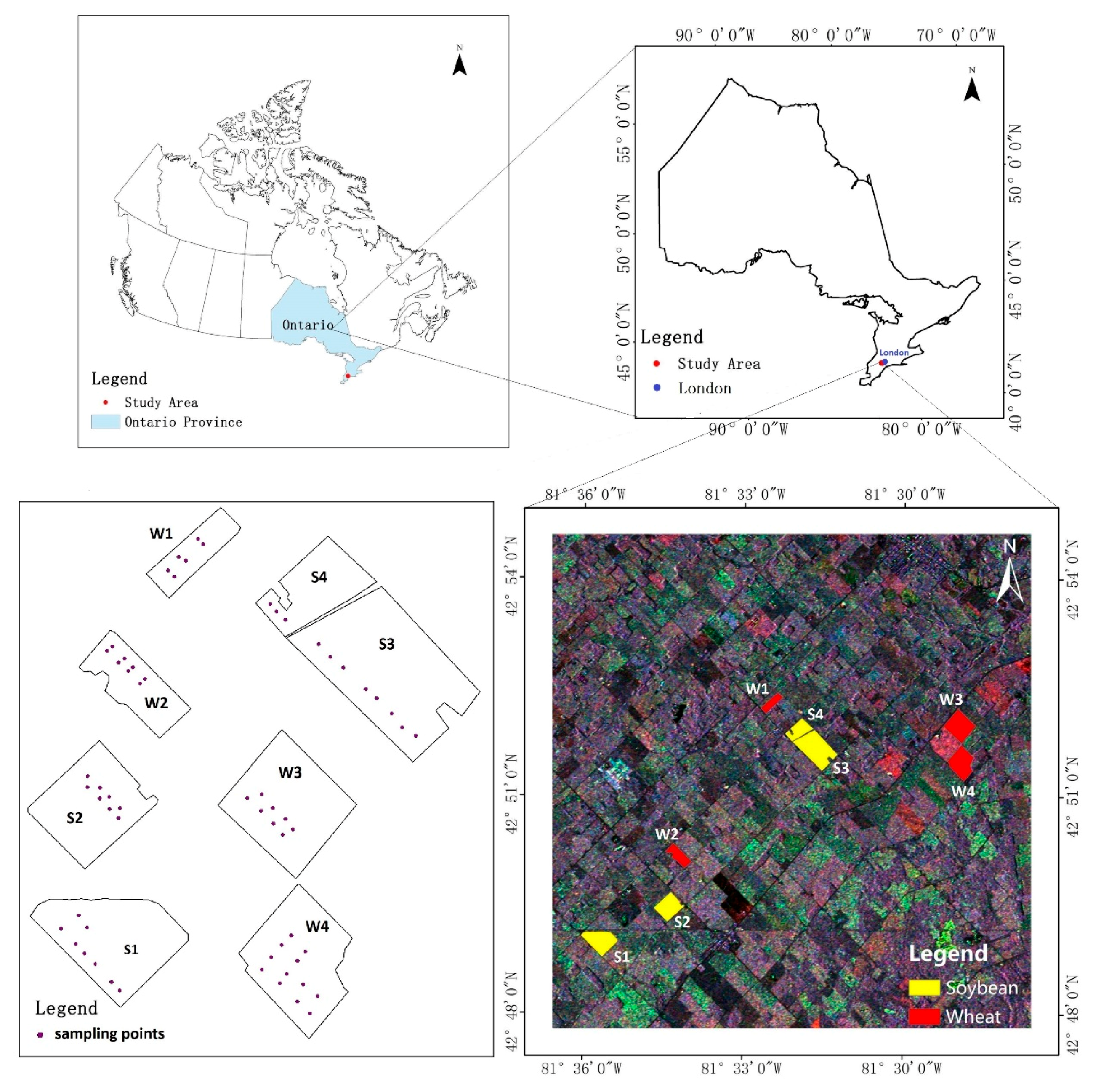
2. Study Site and Data Collection

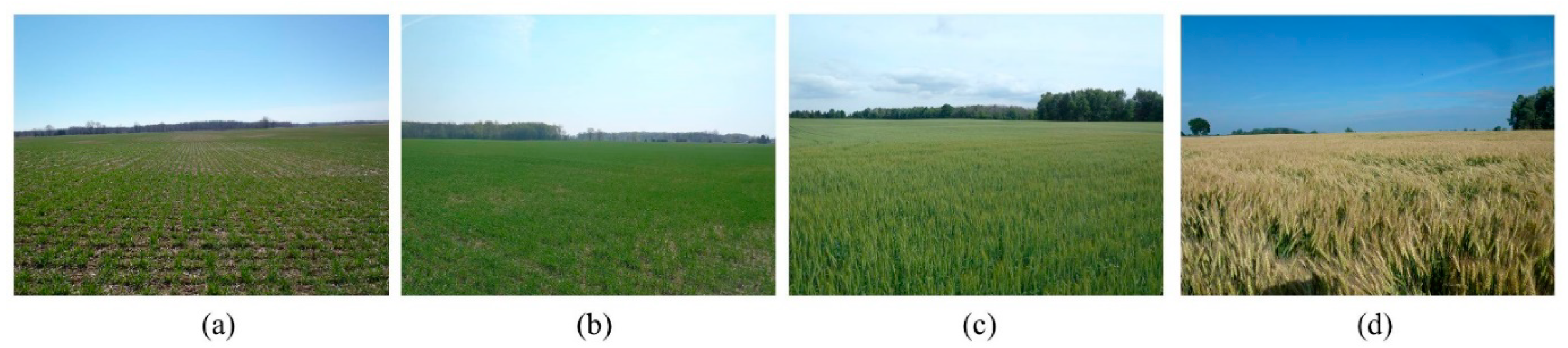
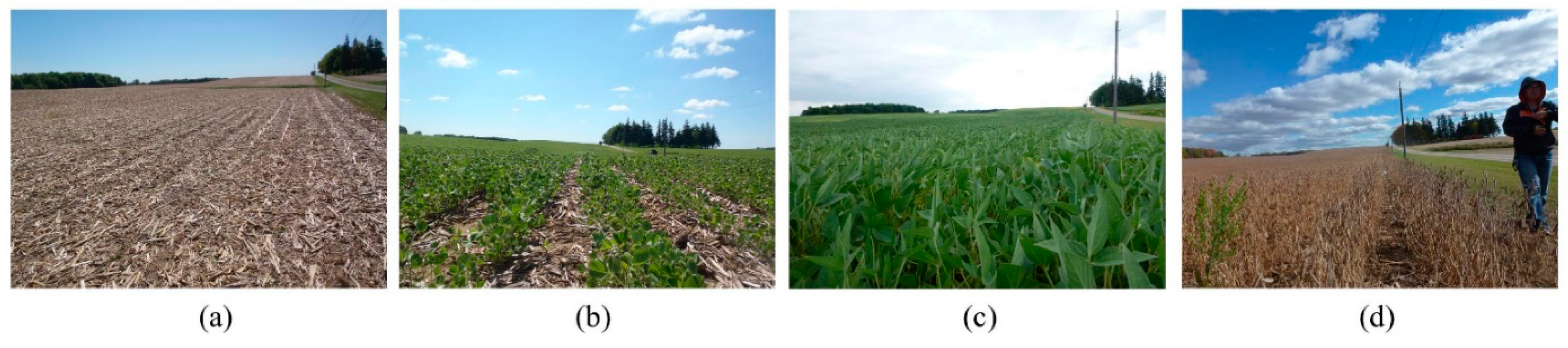
2.1. Ground Truth Data Collection

The study area is located in southwest Ontario near London, Canada (Figure 1). It is an agriculturally productive area in Ontario. The dominant crops are winter wheat, corn, and soybean [41]. There are also some alfalfa and hay growing in this area [42]. Winter wheat is usually sown in October of the previous year and harvested in late July to early August the following year; whereas, corn and soybean are usually sown in May and harvested in September or October. As the weather gets warmer in April, winter wheat starts to grow. Therefore, field campaign was conducted in the study area from April to October in 2015 simultaneously with each RADARSAT-2 SAR data acquisition. In addition, the study sites were not irrigated over the entire crop growth stages. It is important to note that vegetation coverage was variable throughout the crop growing season. The vegetation cover was fully open or low at the beginning of the season and it became denser as the crops continued to develop. Figure 2 and Figure 3 show sample ground truth photos of soybean and winter wheat.

Within a few hours before or after the RADARST-2 satellite overpasses, ground measurements were regularly collected by Geographic Information Technology and Application (GITA) laboratory at the University of Western Ontario in 2015. For this study, a total of eight fields, including four winter wheat and four soybean fields, were selected for model development and validation. Multiple sampling sites were deployed in each of the study fields to capture within-field variability. Three to ten samples were selected in each field, which resulted in 32 wheat and 27 soybean samples per satellite acquisition. Each sample is separated from others with a distance of at least 50 m. The locations of all sample sites were georeferenced while using a global positioning system (GPS) to reference with satellite imagery. Soil and crop measurements were randomly taken within a 10 m by 10 m area of each georeferenced site. SSM was coincidentally measured with each RADARSAT-2 overpass while using a Theta-Probe Soil Moisture Sensor with the soil depth of 0–5 cm by inserting the rods into the ground vertically for all of the sample sites. For each sample, the mean SSM was calculated from six replicate measurements. Within the study area, a total of 236 sampled data were obtained for the 2015 growing season. The measured SSM in the study area covers a wide range of values, from 4.31 [vol.%] to 38.31 [vol.%] in the study area. Surface roughness was collected at early growth stages using a one-meter long needle profiler of 200 pins, with an interval of 0.5 cm between the pins. For the measured surface roughens of the study area, the root mean square (rms) height ranges from 0.63 cm to 3.95 cm, and the correlation length ranges between 8.89 cm and 24.83 cm. The soil texture data were also collected by A&L Canada Laboratories Inc. (https://www.alcanada.com/) during this period. The primary soils are loamy sand, sandy loam, and loam. Soil texture was reported to have an effect on the dielectric behavior over the entire frequency range and is most pronounced at frequencies below 5 GHz [43]. Previous research has found that soil texture effects decreased with increasing radar frequency [44]. In this study, RADARSAT-2 SAR data (C band, 5.405 GHz) was acquired over the study area throughout the growing season. The effect of soil texture on the backscattering coefficient was not considered in this study. Plant area index (PAI) and vegetation coverage were measured at each sample site while using a Nikon D300S camera with a 10.5-mm fisheye lens. The calculation of the PAI is based on Poisson model using gap fraction measurements. More details on fisheye photo collection and subsequent PAI retrieval can be found in Shang et al [45]. Vegetation coverage is defined as the fraction of soil that is covered by vegetation viewed in the nadir direction of the hemispherical photos. The value of vegetation coverage equals to 100% minus the vegetation gap fraction. Vegetation coverage and PAI show a strong exponential relationship (Figure 4). The BBCH (Biologische Bundesanstalt, Bundessortenamt, und CHemische Industrie) phenology and plant height were measured in the general survey. The PAI was not measured at the late growth stages for soybean, as most of the soybean plants had lost their leaves from this point of time (after 13 September). It should be noted that the RADARSAT-2 SAR data were not acquired over the late growth stage of winter wheat and early growth stage of soybean (from 21 May to 16 July 2015,

Table 1. Collected vegetation parameters and soil moisture in the study areas.

Date.	PAI (m3/m3)		Soil Moisture (vol.%)		Vegetation Coverage (%)		BBCH		Crop Height (cm)
	Wheat	Soybean	Wheat	Soybean	Wheat	Soybean	Wheat	Soybean	Wheat	Soybean
6 May 2015	0.29–0.71		13.61–26.52		14.04–32.91		22		10
20 May 2015	0.52–0.81		6.42–24.21		21.68–41.93		30		29
17 July 2015		0.81–2.12		14.03–38.31		41.10–61.74		51		35
10 August 2015		1.45–4.52		11.95–34.71		58.81–87.28		70		74
3 September 2015		1.06–3.94		4.31–31.02		46.06–76.87		78		85
13 September 2015		2.20–2.77		9.53–21.79		50.61–64.35		82		103
17 September 2015				6.99–18.62		40.13–50.03		87		97
27 September 2015				4.31–15.12		27.82–34.41		97		82
1 October 2015				7.45–26.28		19.53–24.47		99		80

) due to the access conflicts of users.

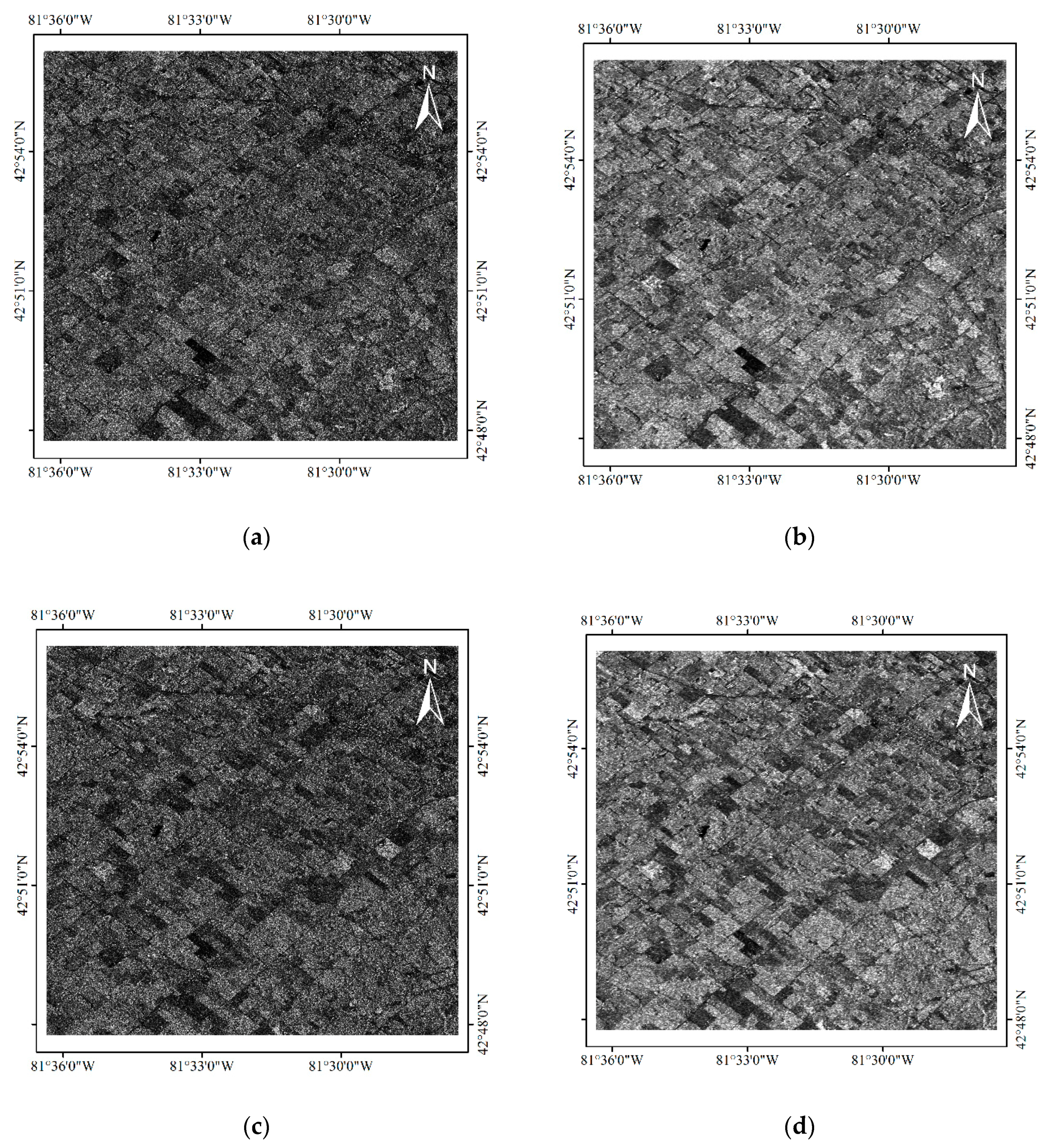
2.2. RADARSAT-2 Data

RADARSAT-2 is a C-band (approximately 5.6 cm wavelength) SAR sensor onboard with multiple configurations and polarization modes. RADARSAT-2 fine beam quad-polarized data with a nominal spatial resolution of 8 m (range resolution: 5.2 m; azimuth resolution: 7.7 m) were acquired over the study area throughout the 2015 growing season (

Table 2. Characteristics of acquired RADARSAT-2 data.

Date and Local Time	Orbit	Beam	Incidence Angle (deg.)
6 May 2015 18:15	Ascending	FQ10	28.39-31.57
20 May 2015 18:07	Ascending	FQ1	17.49-21.15
17 July 2015 18:15	Ascending	FQ10	28.39-31.57
10 August 2015 18:15	Ascending	FQ10	28.39-31.57
3 September 2015 18:15	Ascending	FQ10	28.38-31.57
13 September 2015 18:23	Ascending	FQ20	38.64-41.27
17 September 2015 18:07	Ascending	FQ1	17.49-21.15
27 September 2015 18:15	Ascending	FQ10	28.39-31.57
1 October 2015 06:39	Descending	FQ9	27.29-30.53

). The local overpass time of the ascending and descending direction is afternoon and morning, respectively (Table 2). A geometric correction model [46] was used for the geometric correction of the RADARSAT-2 SAR images, resulting in an accuracy of around one pixel in both X and Y directions. The images were converted to backscattering coefficient (${\sigma }^o$) while using Next ESA SAR toolbox (NEST) that was provided by the European Space Agency (ESA). For speckle noise reduction, a refined Lee filter [47] with a window size of 5 × 5 pixels was applied to the SAR data. Figure 5 illustrates the filtered RADARSAT-2 SAR images over the study area. The original intensity images were blemished with the speckle noise at both HH and VV polarizations. Figure 5a,d show that the speckle noise was sufficiently suppressed. To quantitatively analyze the effect of the Lee filter on the SAR images, the common measure for estimation of speckle level in the image, the equivalent number of looks (ENL) was selected. For HH polarization, ENL increased from 1.16 to 20.31; for VV polarization, ENL increased from 1.10 to 19.74. A high value for ENL indicates that the speckle was effectively suppressed [48]. It should be noted that the value of ENL is usually less than the actual number of looks as a result of spatial correlation [48]. Subsequently, the RADARSAT-2 SAR images were resampled to 10 m × 10 m. At different incidence angles, a corresponding SAR signal will exhibit different response to soil moisture. The available dataset has the incidence angle, ranging from 17.49° (FQ1) to 41.27° (FQ20) (Table 2). As the polarization signature can be affected by the incidence angle, a normalization was performed at a reference incidence angle to make the SAR backscattering comparable in order to reduce the effect of local incidence angle effect on the backscatter coefficients [2]. The radar backscattering can be normalized to any other angle using [49]:

$${\sigma }_{\theta ref}^0={\sigma }^0\frac{{\cos }^n\theta ref}{{\cos }^n\theta },$$

(1)

where $\theta$ is the incidence angle, ${\sigma }^0$ is the backscattering observation at incidence angle, ${\sigma }_{\theta ref}^0$ is the normalized backscattering coefficient, and $\theta ref$ is the reference incidence angle, in this case chosen to be 30°. The power index, n, is defined as the slope of a linear fit between $\ln ({\sigma }^0)$ and $\ln (\cos \theta )$. The n values varied between 0.2 and 3.4, depending on vegetation type and season [49].

3. Methods

3.1. Soil Surface Backscattering

The Dubois model was employed in this study to determine the backscattering of the underlying soil of agricultural fields. Dubois model quantifies the backscattering coefficient from a surface as a function of its roughness parameters (root mean square (RMS) height), its dielectric constant, and the characteristics of the acquired images (polarization, incidence angle, and wavelength). The backscattering coefficient at HH polarization (${\sigma }_{HH}^o$) and VV polarization (${\sigma }_{VV}^o$) are expressed as

$${\sigma }_{HH}^o={10}^{-2.75}({\cos }^{1.5}\theta /{\sin }^5\theta ){10}^{0.028\epsilon \tan \theta }{(ks\sin \theta )}^{1.4}{\lambda }^{0.7}$$

(2)

$${\sigma }_{VV}^o={10}^{-2.35}({\cos }^3\theta /{\sin }^3\theta ){10}^{0.046\epsilon \tan \theta }{(ks\sin \theta )}^{1.1}{\lambda }^{0.7}$$

(3)

where $\theta$ is the incidence angle; $\epsilon$ is the relative dielectric constant. $k$ is the free space wave number given by $k=2\pi /\lambda$, $\lambda$ is the wavelength in cm; $s$ is the RMS height of the surface roughness (cm).

The Dubois model was originally developed to describe the scattering from bare soil only; therefore, vegetation backscattering effects were not incorporated in the model. This model was found to underestimate SSM and overestimate RMS height over vegetated surfaces [50].

3.2. Effect of Vegetation

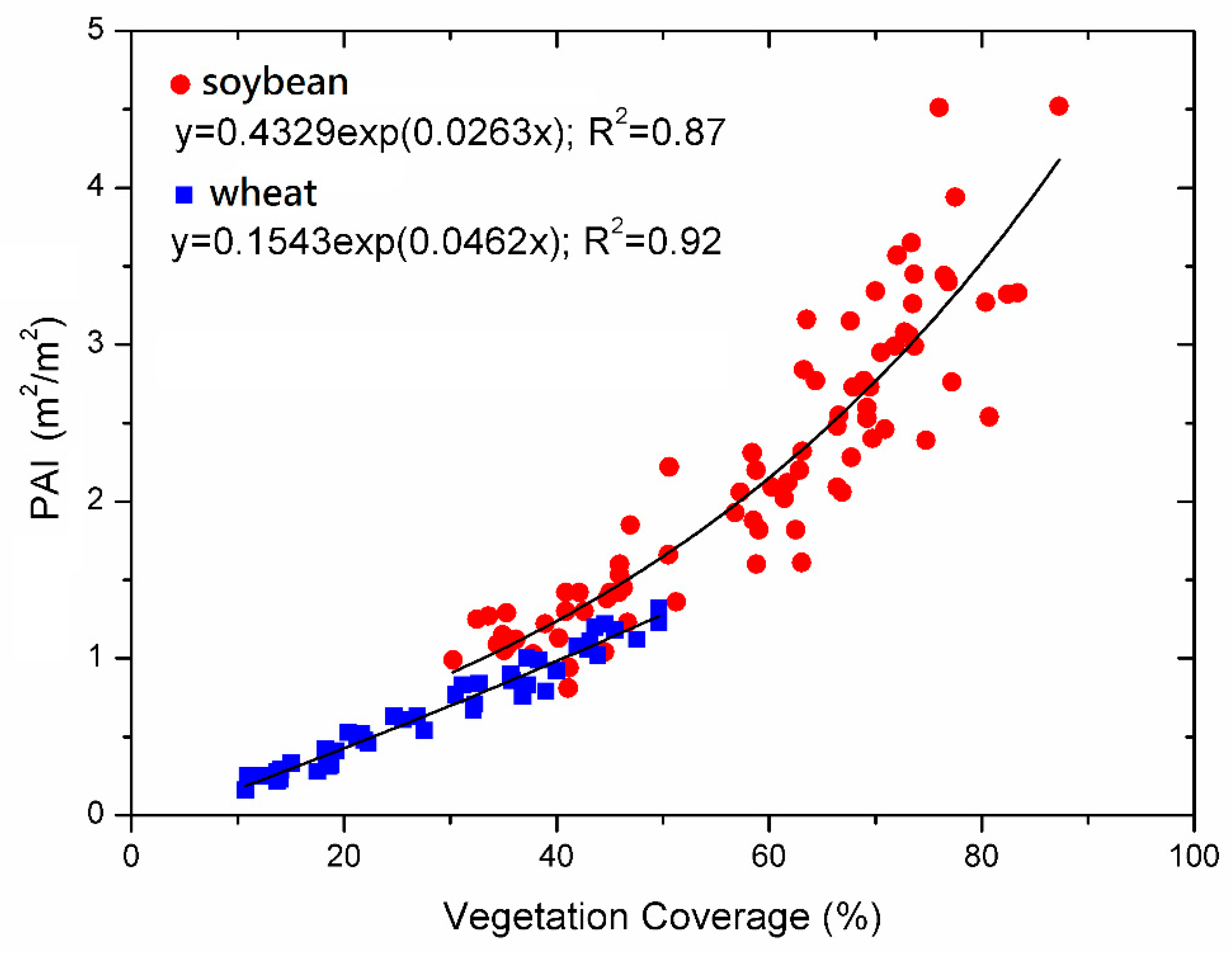
3.2.1. Vegetation Backscattering

Radar backscattering responds to both surface roughness and SSM over bare soil. However, over agricultural fields, vegetation cover and vegetation characteristics also affect it [51]. The backscattering over the vegetated field is the sum of volume scattering from the vegetation and the surface scattering from the underlying soil. In addition, the backscattering from the underlying soil is attenuated by the vegetation canopy. Therefore, backscattering from the vegetation canopy should be removed to retrieve the SSM. In this study, the WCM was used to reduce the effect of vegetation. The WCM assumes that vegetation consists of a collection of spherical water droplets that are structurally held in place by dry matter [52]. In the WCM, the total backscattering (${\sigma }^o$) is represented as the incoherent sum of the contributions from the vegetation (${\sigma }_{veg}^o$) and the underlying soil (${\sigma }_{soil}^o$), which is attenuated by the vegetation layer. For the whole canopy, WCM can be expressed as

$${\sigma }_{pp}^o={\sigma }_{pp,veg}^o+{\tau }^2{\sigma }_{pp,soil}^o,$$

(4)

$${\sigma }_{pp,veg}^o=AV\cos \theta (1-{\tau }^2),$$

(5)

$${\tau }^2=\exp (-2BV/\cos \theta ),$$

(6)

In these equations, ${\tau }^2$ is the two way attenuation through the canopy layer, pp is the polarization mode (pp = HH or VV). A and B are model coefficients that depend on canopy type that need the calibration [53]. V is a descriptor of the vegetation canopy. An important part of the vegetation scattering and attenuation is controlled by the leaves, a widely used descriptor to describe the amount of foliage is PAI when referring to all of the light blocking elements [54,55]. Therefore, the canopy description V were associated with PAI, i.e., V = PAI. To estimate the vegetation parameter A without the roughness, Michigan Microwave Canopy Scattering model (MIMICS) [55] was used to calculate vegetation backscattering coefficients ${\sigma }_{veg}^o$ at the sampling sites where ground-based measurements of soil and other ancillary data are available. Afterwards, the value of A was derived while using the least square method, which is an approach in regression analysis to approximate the solution of overdetermined systems. The attenuation factor ($\tau$) was calculated using the method that was described by Wang [56]. $\tau$ is exponentially related to the extinction coefficient, which is statistically averaged over the spherical orientation probability distribution [56]. Subsequently, the value of B was obtained also using the least square method. The Dubois model was used to simulate soil backscattering in the WCM model. This simulation allows for a more realistic SSM contribution in the total backscattering of Equation (4). The WCM can be further simplified by expanding the attenuation factor ${\tau }^2$ while using the Maclaurin series [38]:

$${\tau }^2=\exp (-2BV/\cos \theta )=1-\frac{2BV}{\cos \theta }+\frac{2B^2{V}^2}{{\cos }^2\theta }+\cdots ,$$

(7)

Combining Equations (7), if only the first two items are preserved in Equation (4), the WCM can be simplified as:

$${\sigma }_{pp}^o=2AB{V}^2+(1-2BV/\cos \theta ){\sigma }_{pp,soil}^o,$$

(8)

A variable substitution is conducted to further simplify Equation (8):

$${\sigma }_{pp}^o=a{V}^2+bV{\sigma }_{pp,soil}^o+{\sigma }_{pp,soil}^o,$$

(9)

With $a=2AB$ and $b=-2B/\cos \theta$ as the model coefficients.

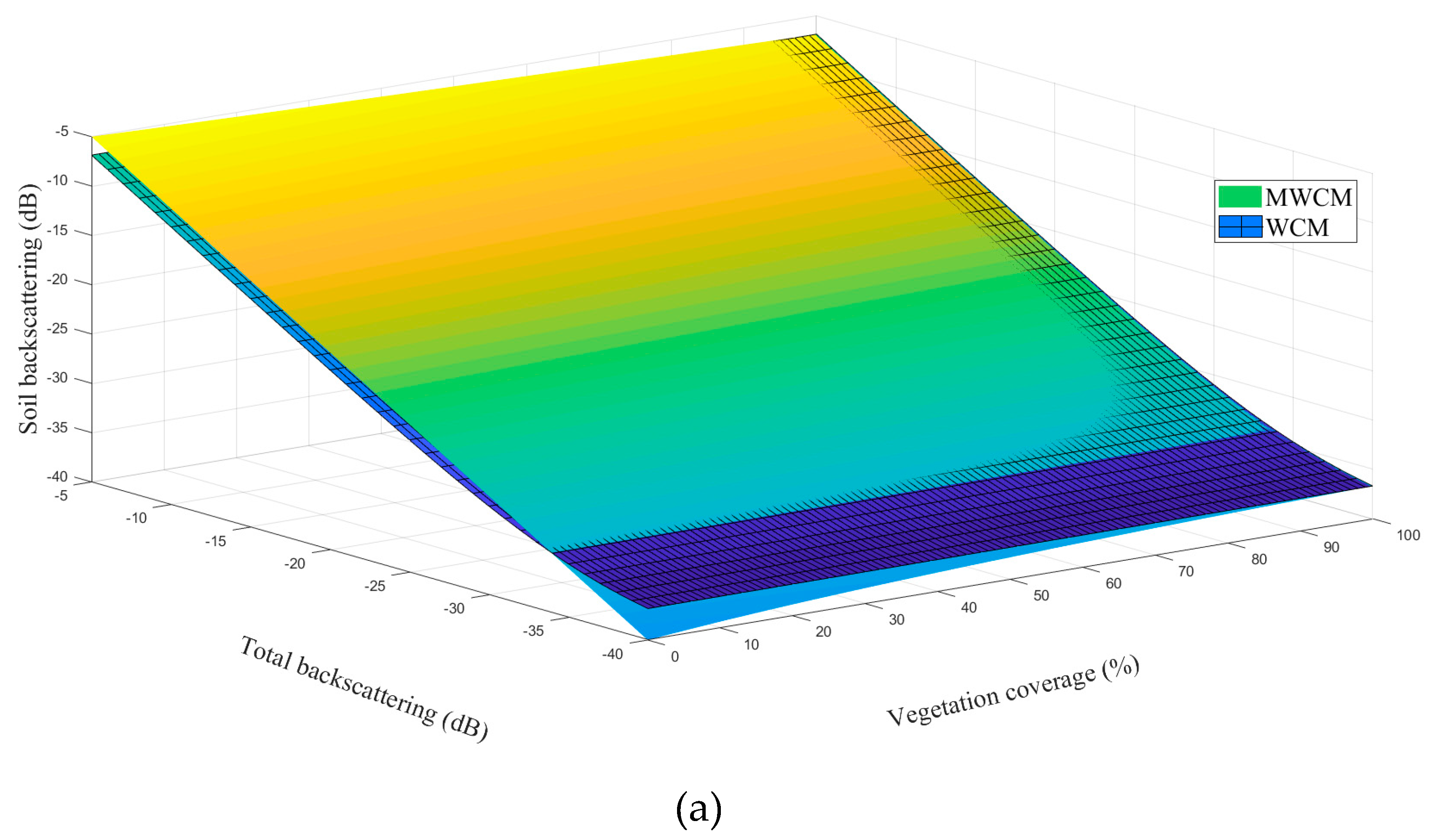
3.2.2. A Modified Model of Vegetation Backscattering

One assumption of the WCM is that volume scattering is the predominant mechanism that is responsible for the backscattering from vegetation canopy [36]. However, at early growing stages, crop is usually sparse, but this assumption is not always satisfied. To address this issue, a modified Water Cloud Model (MWCM) was developed in this paper. The backscattering contribution of bare soil surface must be considered as a key component of the total backscattering due to the strong influence of underlying surface over sparsely vegetated area. In previous studies [57,58], the scattering mechanism for the vegetation cover and bare soil components in a pixel were separated by vegetation coverage. Soil and the vegetation effects are assumed to be independent to simplify the different processes contributing to the total backscattering. Scattering from the interaction between soil and vegetation canopy is neglected. The backscattering coefficient that is measured over agricultural field is described as the sum of soil and canopy contributions weighted by the vegetation fractional cover. First, the backscattering was calculated while using a vegetation backscattering model under the assumption that a pixel was fully covered by vegetation. Subsequently, the actual backscattering coefficient from the fraction of the surface covered by vegetation was calculated while using the vegetation coverage. Similarly, the backscattering coefficient for the fraction representing direct backscattering from the bare soil surface was calculated based on the fraction of the bare soil. Therefore, the total backscattering from a pixel can be expressed as:

$${\sigma }_{pp,total}^o=f_{veg}{\sigma }_{pp}^o+(1-f_{veg}){\sigma }_{pp,soil}^o,$$

(10)

where $f_{veg}$ is the vegetation coverage. ${\sigma }_{pp,soil}^o$ was calculated using the Dubois model.

Combining Equations (9), Equation (10) can be rewritten as:

$${\sigma }_{pp,total}^o=f_{veg}(a{V}^2+bV{\sigma }_{pp,soil}^o)+{\sigma }_{pp,soil}^o,$$

(11)

Figure 4 shows a strong relationship between LAI and vegetation coverage. The PAI could be expressed by the vegetation coverage.

$$PAI=0.3383\exp (0.0278f_{veg}),$$

(12)

The canopy description V were associated with PAI, i.e., V = PAI. Subsequently, Equation (11) can be rewritten as:

$$\begin{array}{ll}{\sigma }_{pp,total}^o=& f_{veg}[a{(0.3383\exp (0.0278f_{veg}))}^2\\ & +b\times 0.3383\exp (0.0278f_{veg}){\sigma }_{pp,soil}^o]+{\sigma }_{pp,soil}^o\end{array}$$

(13)

Further, ${\sigma }_{pp,soil}^o$ can be solved.

$${\sigma }_{pp,soil}^o=\frac{{\sigma }_{pp,total}^o-a{f}_{veg}{\left[0.3383\exp (0.0278f_{veg})\right]}^2}{b{f}_{veg}\times 0.3383\exp (0.0278f_{veg})+1},$$

(14)

3.3. Retrieval of Surface Soil Moisture

In many studies, the estimation of soil moisture was accomplished while using a priori knowledge of surface roughness [50]. However, soil surface roughness is difficult to be measure once the crop starts to develop. To overcome this limitation, an inversion scheme was developed using the dual co-polarizations (HH and VV) from the quad polarization RADARSAT-2 SAR data. The effect of vegetation can be eliminated from Equation (14) by combining the simulated bare soil surface contribution and observed backscattering coefficient. After minimizing the effect of vegetation on the backscattering coefficient by the MWCM, to eliminate the influence of the surface roughness, the retrieved dielectric constant of soil can be achieved by using HH and VV polarizations backscattering coefficients as inputs to the Dubois model [50]:

$$\epsilon =\frac{1}{0.024\tan \theta }{\log }_{10}\left(\frac{{10}^{0.19}{\lambda }^{0.15}{\sigma }_{HH,soil}^o}{{(\cos \theta )}^{1.82}{(\sin \theta )}^{0.93}{({\sigma }_{VV,soil}^o)}^{0.786}}\right),$$

(15)

The volumetric SSM can be retrieved through the dielectric constant while using the equation developed in [59]:

$$m_v=-5.3\times {10}^{-2}+2.92\times {10}^{-2}\epsilon -5.5\times {10}^{-4}{\epsilon }^2+4.3\times {10}^{-6}{\epsilon }^3,$$

(16)

Overall, to retrieve the SSM from RADARSAT-2 SAR data that were collected during the wheat and soybean growing season at the pixel scale, the retrieval procedure includes a correction of surface roughness and vegetation cover effects. The vegetation effects are corrected by the MWCM. The roughness correction is based on the dual polarizations (HH and VV) of RADARSAT-2 SAR data. As the validity range of the Dubois model is constrained within ${30}^{°}\le \theta <{60}^{°}$, the range of validation data does not include the incidence angle below ${30}^{°}$. Thus, normalization is performed with respect to a reference incidence angle of ${30}^{°}$, as described in Section 2.2. Subsequently, SSM estimation is performed by applying the relationship between volumetric SSM and dielectric constant of soil.

4. Results and Discussion

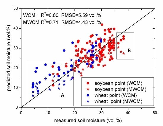
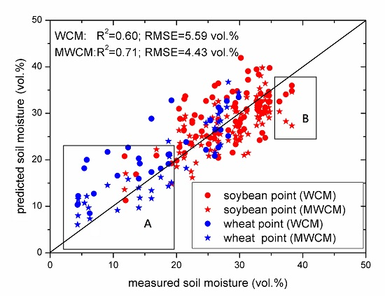
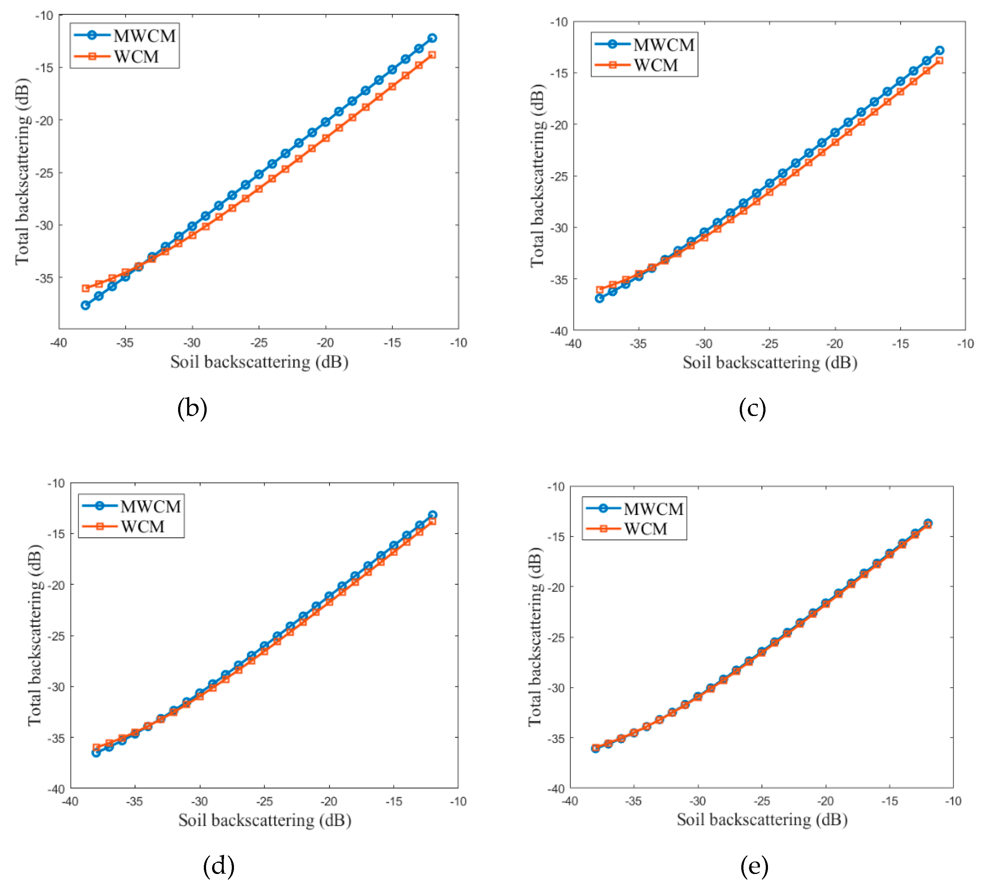
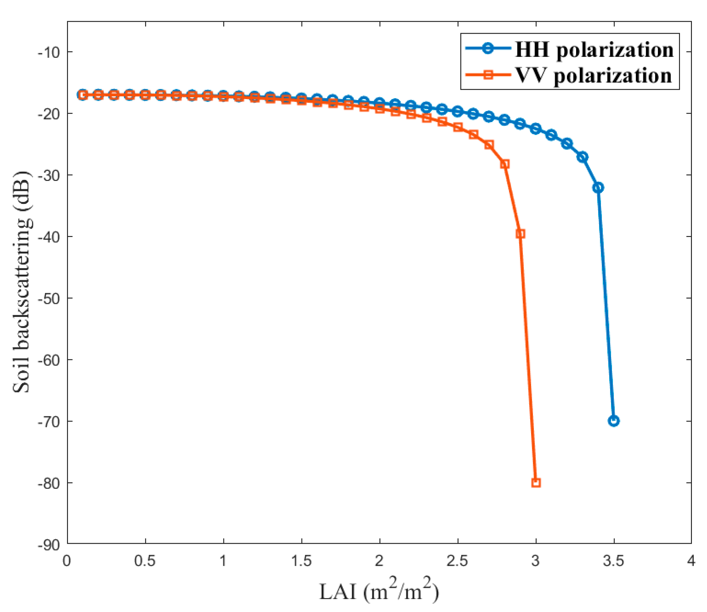
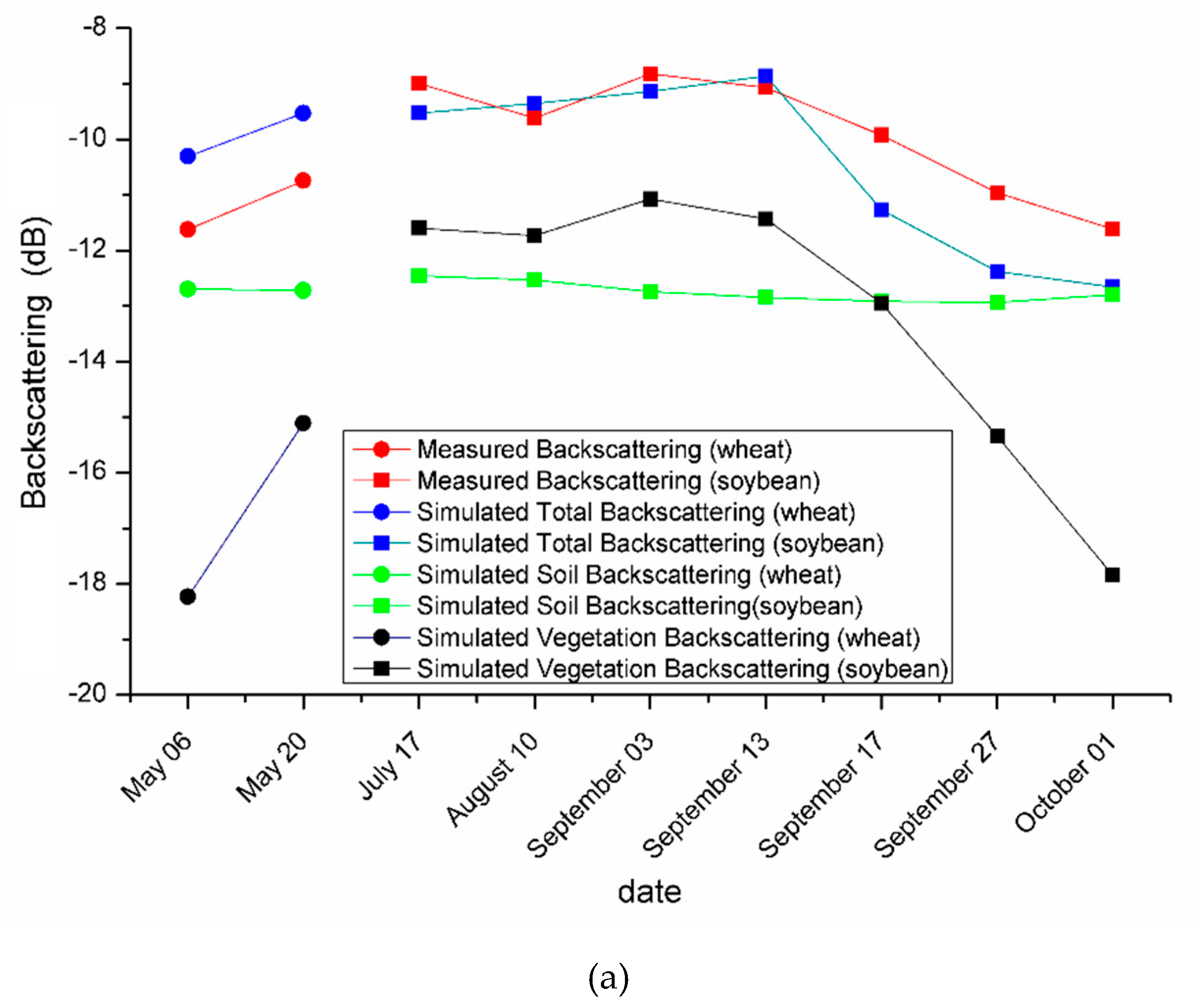
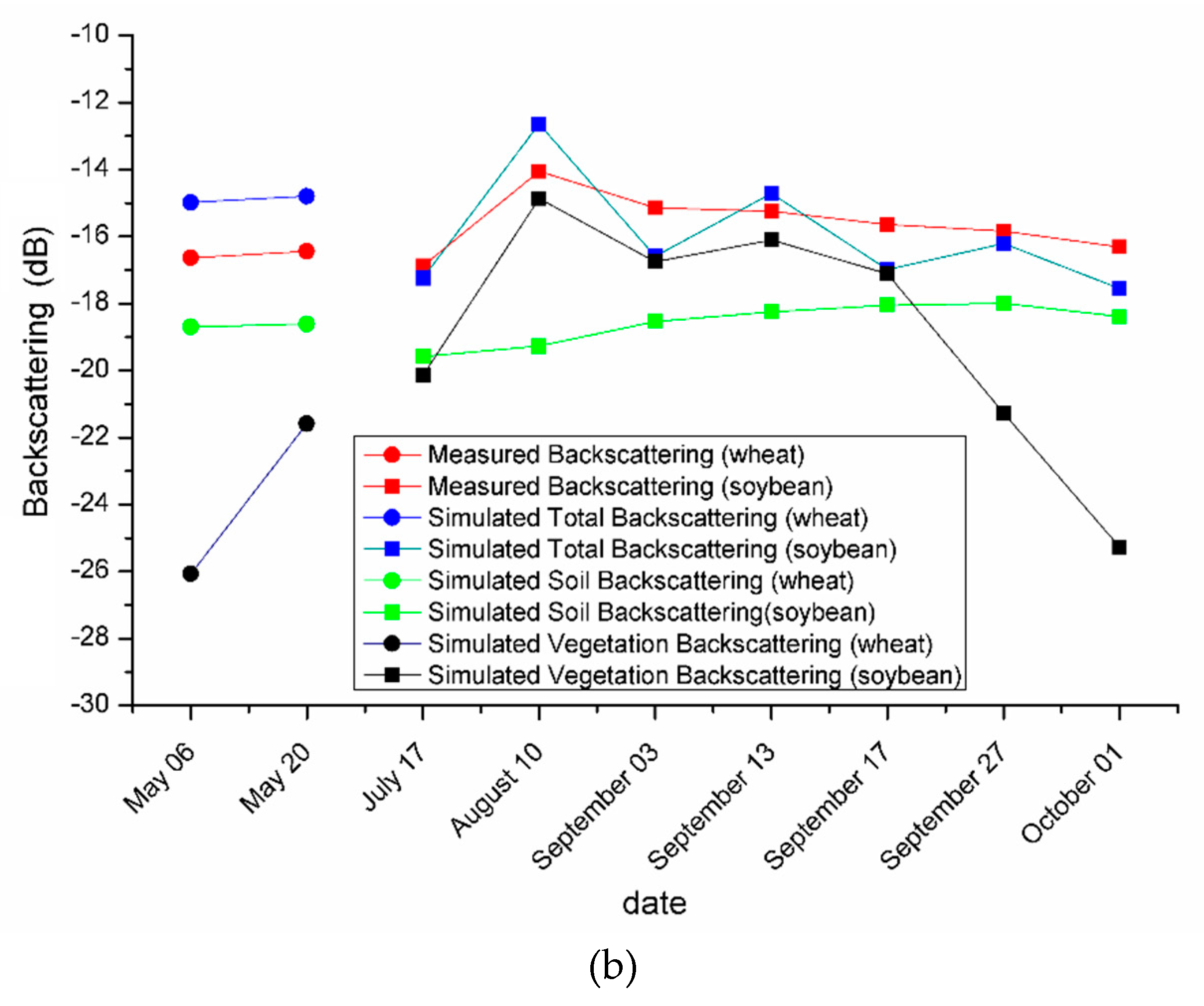
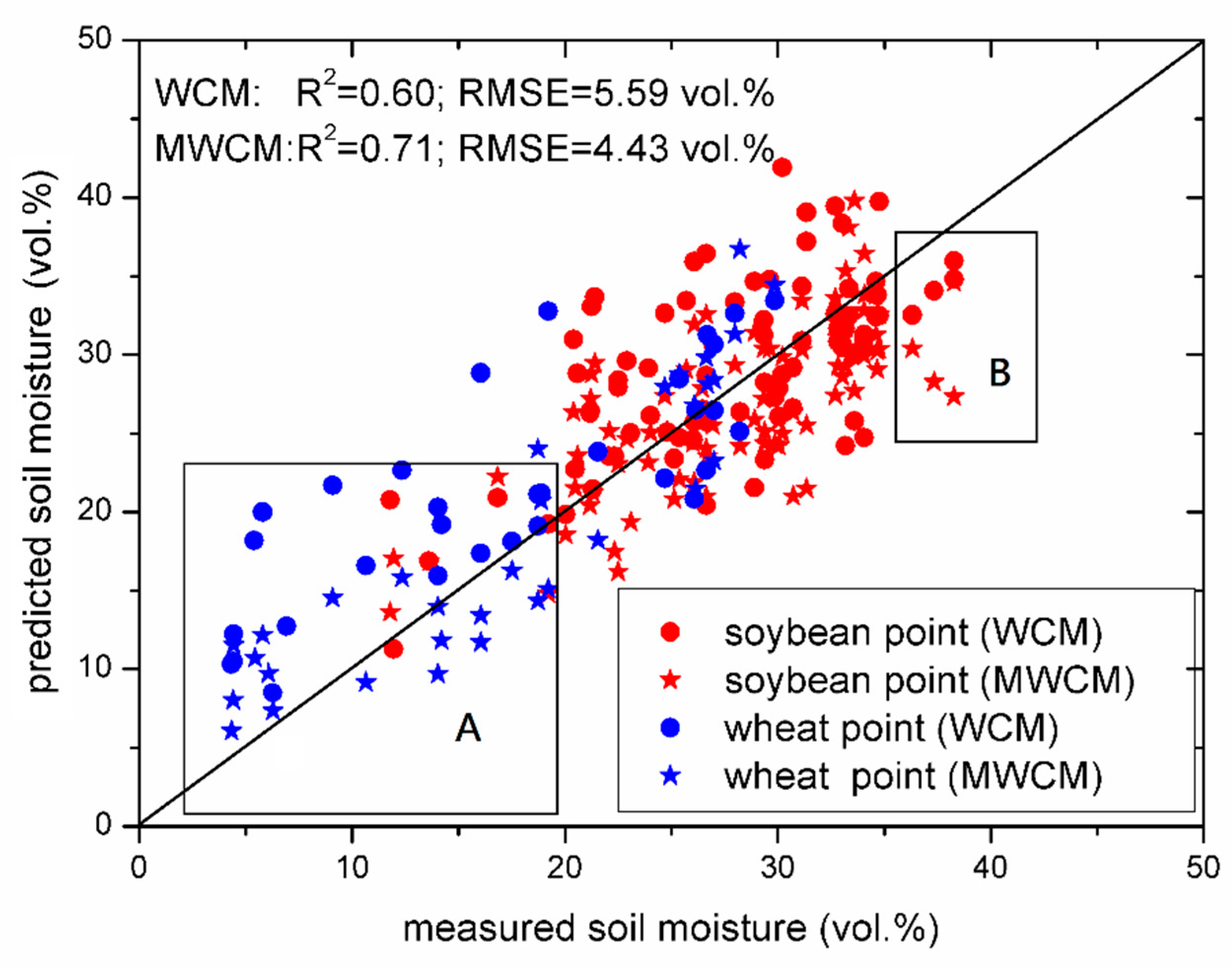
4.1. Perfomance of MWCM

To compare the MWCM and WCM under different vegetation coverage, the behaviors of MWCM and WCM were studied as a function of vegetation coverage and PAI in HH polarization. The PAI in both models was estimated while using vegetation coverage (See Equation (12)). Figure 6a–e depicts the behaviors of backscattering as a function of vegetation coverage using the WCM and MWCM, respectively. The figure clearly shows that the radar signal is sensitive to vegetation coverage in both MWCM and WCM. The simulated soil backscattering coefficients using WCM and MWCM are nearly the same when vegetation coverage is greater than 90% (Figure 6e). They are similar to each other when vegetation coverage is between 60% and 90% (Figure 6d,e). They diverge from each other when the vegetation coverage is less than 60% (Figure 6b,c). When the total backscattering coefficient is greater than −33 dB, the soil backscattering coefficient that is simulated by MWCM more significantly decreases than that simulated by WCM with the increase of vegetation coverage. When the total backscattering coefficient is less than -33 dB, the backscattering coefficient that is simulated by MWCM is less than that simulated by WCM. Note that, in the case of bare soil, when the vegetation coverage is 0%, the total backscattering coefficient and the soil backscattering coefficient simulated by MWCM is equal to each other (Figure 6a). However, in the case of bare soil, the soil backscattering coefficient that is simulated by WCM is greater than the total backscattering coefficient. This indicates that MWCM is more sensitive to vegetation cover; therefore, it is a more suitable model under sparse vegetation cover conditions when compared with WCM.

The soil backscattering was simulated using MWCM to quantify the performance of the proposed model under different PAI values (Figure 7). Figure 7 shows that soil backscattering decreases with an increase in PAI at both HH and VV polarizations. For HH polarization, soil backscattering exhibits a nearly vertical response once the PAI exceeds about 3.5 m²/m². Soil backscattering at VV polarization has the same trend once the PAI exceeds about 3.0 m²/m². It suggests that the SAR signal reaches saturation when the PAI is greater than 3.5 m²/m² for HH polarization and 3.0 m²/m² for VV polarization. It also suggests that HH polarization penetrates the vegetation canopy deeper than VV. The radar signal is unable to penetrate the vegetation, and the soil contribution can be negligible when the backscattering reaches saturation. Therefore, retrieval of SSM while using SAR data will become unreliable at high vegetation biomass.

Figure 8 presents the time series backscattering modeling at both HH and VV polarizations using the MWCM. The soil backscattering is simulated from the Dubois model presented in Section 3.1. The vegetation backscattering is simulated using MWCM. Figure 8 shows that vegetation contributes to the total backscattering, and it will influence the retrieval of SSM. Vegetation backscattering varies throughout the crop growth cycle. The simulated total backscattering coefficient is overestimated at the early growth stage of wheat at both HH and VV polarizations (6 May and 20 May) (Figure 8a,b). The simulated total backscattering coefficient is underestimated at the late growth stage of soybean (from 17 September to 1 October) (Figure 8a,b). It may indicate that the retrieval of soil moisture is affected by crop growth stage.

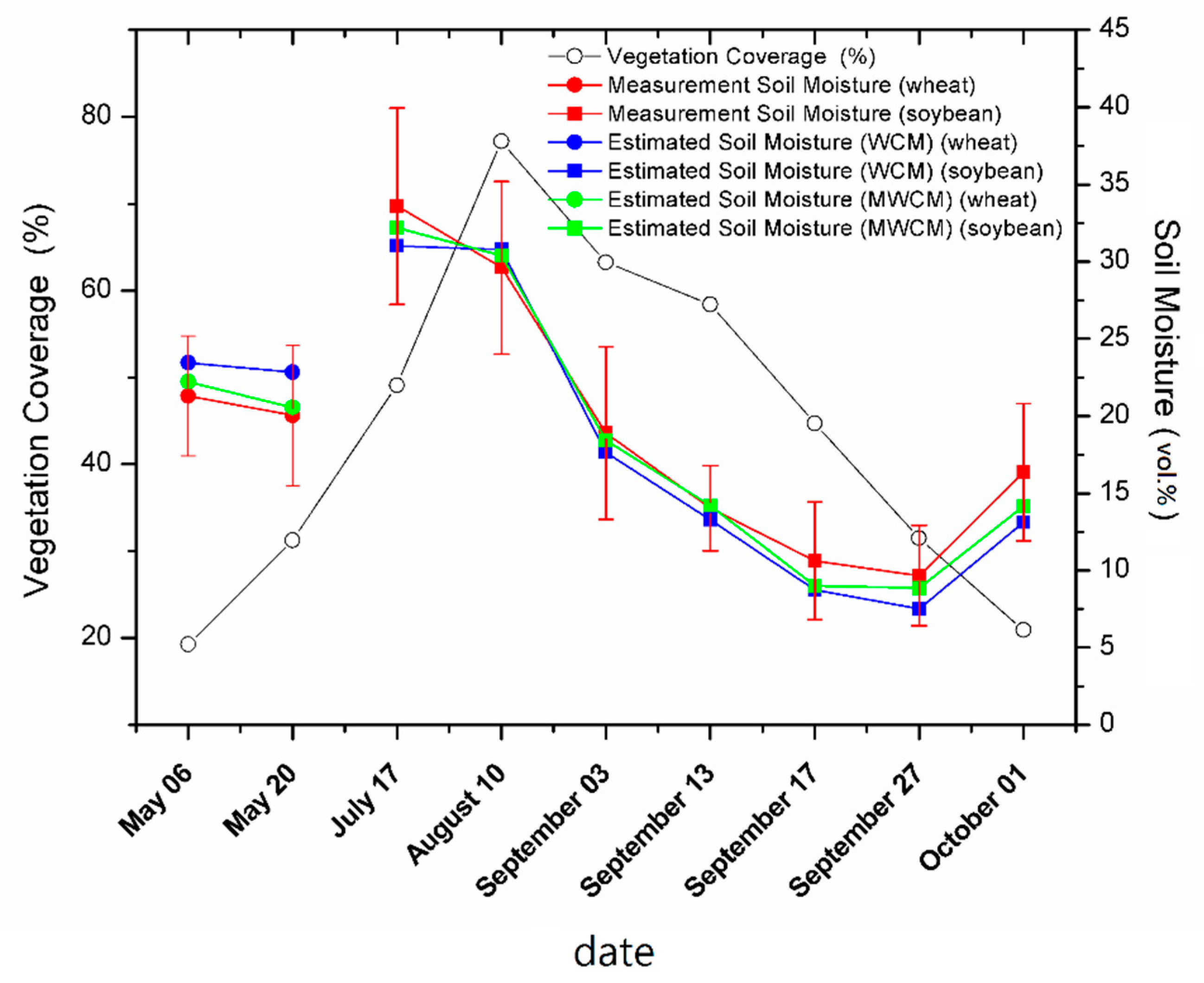
4.2. Retrieval of Soil Moisture

Half of the data points from field surveys were randomly selected and used to calibrate the MWCM. The remaining half of the dataset was used for model validation. Figure 9 shows the resultant inversion of SSM while using the WCM and MWCM to reduce the effect of vegetation. For WCM, the relationship between the measured and predicted SSM is linear (Figure 9) with a moderate correlation (R² = 0.60, p < 0.01, RMSE = 5.59 vol.%). We observed that most of the estimated SSM was overestimated over the wheat fields, especially when the SSM is less than 20 vol.% (Rectangle A in Figure 9). This phenomenon mainly occurred at early growth stages of wheat (BBCH less than 30). The radar backscattering for crops is dominated by direct scattering from the soil in early stage, and the vegetation volume scattering is negligible. The soil contribution to the total backscattering is relatively strong at the early growth stages due to low vegetation coverage [60]. When vegetation is sparse at the early stage, the backscattering increase rate from vegetation exceeds the soil backscattering reduction, due to vegetation attenuation [61]. The backscattering contribution of bare soil must be considered as a primary component in the total backscattering due to the large vegetation gap. With the development of canopy, the backscattering contribution of soil gradually weakens and then reaches the minimum values at peak biomass. When vegetation is sparse, the vegetation gap information was not considered by WCM. Therefore, the SSM was overestimated by the WCM at the early growth stage.

In view of the sparse and patchy vegetation pattern during the crop growing season, the MWCM takes the backscattering of the complementary soil fraction into account. Figure 9 shows the resultant inversion of SSM while using the MWCM when considering the backscattering contribution from the bare soil as a component in the total backscattering. The predicted SSM that was achieved by the MWCM showed that the correlations between the measured and predicated SSM improved by including the effect of bare soil during the agriculture growth season (R² increased from 0.60 to 0.71 and the RMSE decreased from 5.59 vol.% to 4.43 vol.%), especially during the early growth stage of the wheat fields (BBCH less than 30). This suggests that the MWCM has higher sensitivity to soil moisture at relatively sparse vegetation conditions. The MWCM achieves higher accuracy in soil moisture estimation. The result demonstrates that the use of vegetation cover fractions could separate the scattering mechanisms of the fractions of vegetation cover and bare soil, and the accuracy of the SSM estimation was significantly improved.

A linear relationship between the estimated and measured SSM (Figure 9) was observed; it revealed that the method proposed here could effectively estimate SSM over agriculture fields during the growing season. However, as shown in Figure 9, the SSM values in the wet area (SSM greater than 35 vol.%) was underestimated (Rectangle B, Figure 9). This may be due to the high sensitivity of SAR backscattering to changes in SSM with low soil water content (SSM less than 20 vol.%). However, the SAR backscattering is less sensitive to soil moisture for wet soil (SSM greater than 35 vol.%) [62]. This behavior may also be explained through the saturation of SAR’s sensitivity to dielectric permittivity under very wet conditions (SSM greater than 35 vol.%) [30,63]. It may also suggest that this method is problematic for estimating SSM under wet conditions (SSM greater than 35 vol.%).

To better understand the behavior of the model under different vegetation conditions, prediction accuracy (RMSE), and goodness of fit (R²), the achieved results are reported in

Table 3. Performance achieved on test samples (x represents the predicted soil moisture, y represents the measured soil moisture).

Crop Coverage	Model	Regression Function	R2	RMSE [vol.%]
fveg more than 60%	WCM + Dubois	y = 0.837x + 5.579	0.64	5.22
	MWCM + Dubois	y = 0.8954x + 1.721	0.72	4.09
fveg less than 60%	WCM + Dubois	y = 0.6871x + 7.872	0.33	7.13
	MWCM + Dubois	y = 0.7242x + 4.536	0.66	5.19

. As observed in Table 3, the estimated soil moisture using MWCM shows a significant improvement when the percent vegetation cover is less than 60%, which implies that the modified model had higher sensitivity to relatively sparse vegetation condition. However, the accuracy did not significantly vary under relatively dense vegetation conditions (the vegetation coverage is greater than 60%). This is likely, because bare soil contributes little in the total backscattering (the bare soil contribution to the total backscattering was negligible) under relatively dense vegetation conditions.

Figure 10 shows the time-series comparisons of predicted SSM averages and measured SSM averages. The time series of soil moisture show that the retrieval has sensitivity issues during the crops growing season. We observed that the predicted soil moisture was overestimated on 6 May and 20 May. Generally, good agreement was observed between the measured and retrieved soil moisture values, and the retrieval while using MWCM was better than using WCM.

The bias and unbiased root mean square error (ubRMSE) were calculated for retrieved SSM using MWCM and WCM with in situ soil moisture data. As shown in

Table 4. Bias and unbiased root mean square error (ubRMSE) between the measured and estimated soil moisture. Note that the bias and ubRMSE are only for wheat on May 06 and May 20 and only for soybean on other dates.

		May 06	May 20	July 17	Aug. 10	Sep. 03	Sep. 13	Sep. 17	Sep. 27	Oct. 01
Vegetation coverage (%)		19.27	31.25	49.1	77.2	63.26	58.41	44.72	31.52	20.91
WCM	bias	3.39	3.79	−1.48	0.65	−0.67	−0.79	−2.87	−3.14	−4.24
	ubRMSE	7.36	7.55	5.69	4.56	4.56	4.58	7.13	7.25	8.78
MWCM	bias	2.79	2.42	−1.15	0.32	−0.52	0.55	−2.61	−2.81	−4.18
	ubRMSE	5.38	5.19	4.74	3.61	3.63	3.63	5.29	5.39	6.22

, positive bias was obtained for both WCM (3.392 vol.% and 3.795vol.% ) and MWCM (2.793 vol.% and 2.424 vol.%) on 6 May and 20 May 2015. Negative bias was obtained for both WCM (−4.233 vol.%–−2.873 vol.%) and MWCM (−4.182 vol.%–−2.615 vol.%) during the period of 17 September to 1 October 2015. While, in the other period, for WCM, bias had values between −1.485 vol.% and 0.653 vol.%; for MWCM, bias had values between −1.152vol.% and 0.557 vol.%. As shown in Table 4, the ubEMSE had value between 4.577 vol.% and 8.785 vol.% for WCM and MWCM had value between 3.611 vol.% and 6.217 vol.%. Table 4 shows that positive bias was obtained for both WCM (3.392 vol.% and 3.795vol.% ) and MWCM (2.793 vol.% and 2.424 vol.%) on May 06 and May 20. A positive bias suggests that the retrieved soil moisture is systematically overestimated when compared with the ground measurements. This phenomenon may be explained by the strong influence of vegetation. When vegetation is sparse, the backscattering increment from the vegetation exceeds the soil backscattering reduction due to vegetation attenuation [56]. The vegetation is sparse at the early growth stage; it may be because the attenuation on soil backscattering is lower than the increase of vegetation backscattering. Therefore, soil moisture at the early growth stage was overestimated. When comparing with the measured SSM, the SSM retrieval achieves the highest accuracy in the middle of crop growth stage, as shown in Figure 10 and Table 4. It suggests that the WCM is suitable for modeling scattering of dense vegetation conditions. This also indicates that the predominant backscattering from vegetation should be volume scattering when the WCM is applied. It can be observed that soil moisture was underestimated after 17 September (Figure 10 and Table 4). In this study, PAI was used as a vegetation descriptor parameter in WCM. However, vegetation water content also plays an important role in the radar signal. The vegetation dielectric constant represents the maximum capability to store, absorb, and conduct electric energy for vegetation. Over the vegetation canopy, as vegetation moisture content increases, the dielectric constant also increases. Therefore, vegetation that has a larger amount of moisture content will return more energy than drier vegetation, due to the increased dielectric constant. At the beginning of September, vegetation water content decreased due to crop maturity at the late growth stage. The vegetation backscattering was over corrected in WCM. Therefore, the retrieved SSM was underestimated using either WCM or MWCM. However, when comparing with the measured SSM and retrieved SSM, the MWCM achieved higher accuracy than that of WCM.

The results reveal that SSM could be retrieved with a maximum relative error ((measured value − retrieval value)/measured value) of ±81.8% over relatively dry soil condition (soil moisture less than 20 vol.%, Rectangle A in Figure 9). The SSM estimation accuracy is not merely from the model simulation and inversion, but it could also be partially from the data preprocessing. The main error sources causing low accuracy SSM retrieval are attributed to: (1) Errors in the vegetation cover and PAI calculated from fisheye photos may introduce errors into the SSM retrieval. (2) SAR signals that are caused by the speckle noise may introduce errors in SSM retrieval. (3) The acquisition time for the ascending and descending orbits of RADARSAT-2 is different (morning and evening). The presence of dew drops in the morning during descending pass may act to increase the dielectric constant of vegetation [64] and result in overestimated SSM. (4) The effect of soil texture on the backscattering coefficient was not considered in this study and it could be another source of error. It should be clear that all other sources of uncertainty may also increase the uncertainty of the retrieved SSM. However, these sources of error are not severe, and such assessment is out of the scope of the research objective of this paper.

5. Conclusions

The study that was carried out in this paper acknowledges the problem of SSM retrieval over agriculture fields during the growing season. An algorithm aiming at improving the accuracy of SSM retrieval was proposed. The proposed algorithm was developed while using data that were collected over wheat and soybean fields in southwest Ontario, Canada, based on the MWCM and Dubois models. In this study, the MWCM was used to address issues related to sparse and patchy vegetation cover during the crop growth season. The inclusion of vegetation cover fractions satisfied the conditions for the WCM in cases of sparse vegetation cover and improved the SSM estimation because it separated backscattering from soil and vegetation. Results show that the MWCM could provide important information for a wide range of complicated environmental areas and could accurately represent vegetation backscattering in areas that were either fully or partially covered by vegetation. However, it should be noted that monitoring SSM using SAR data is affected by signal saturation when the vegetation biomass is high. An accurate estimation of soil moisture is prohibited when the SAR signal cannot penetrate the dense vegetation canopy (for HH polarization, LAI is greater than 3.5 m²/m²; for VV polarization, LAI is greater than 3.0 m²/m²) (Figure 7). The MWCM is more capable of modeling SAR backscattering for relatively sparse vegetation conditions when compared with the WCM (Figure 6). In the MWCM, the backscattering from vegetation canopy and bare soil within a pixel can be separated. The WCM assumes that vegetation is uniformly distributed, while the MWCM considers the relative low fraction of vegetation cover and adds a backscattering component from the complementary soil fraction.

An attraction of this newly proposed method is that it can estimate soil moisture from SAR data without using the information of soil surface roughness. In this method, crop contribution to the radar response was removed in the MWCM to estimate the SSM using the Dubois model in agriculture fields. Inversion of the Dubois model can be achieved by using HH and VV backscattering coefficients to eliminate the influence of surface roughness. The SSM can then be estimated from RADARSAT-2 data. Validation of the SSM retrievals against ground measurements reveals a good correlation between the measured and estimated SSM (R² = 0.71, RMSE = 4.43 vol.%, p < 0.01). The model underestimates the SSM under wet conditions because of the low sensitivity of the radar backscattering coefficient to high soil moisture contents (SSM greater than 35 vol.%). In general, the retrieved values of SSM are overestimated as compared with the field measurements during early crop growth stages, due to over compensation of backscattering caused by vegetation cover. In contrast, underestimation of the retrieved soil moisture is observed during the late crop growth stage, which is associated with lower vegetation water content at senescence. When comparing with the WCM, soil moisture estimated by MWCM has a stronger correlation with in situ measurements at all times throughout the crop growing season.

Most of the previous studies on SAR backscattering modeling over agricultural fields adopted the unified vegetation assumption [65]. Thus, it was difficult to use these models during the growing season, with vegetation cover ranging from relatively sparse to dense. In the newly proposed method, vegetation coverage is incorporated into the model to calculate the contributions from both vegetation and bare soil at pixel level to precisely capture the differences of the scattering mechanisms between vegetation and bare soil. The validation results demonstrate that the proposed method has good potential for SSM retrieval of soils agriculture fields during the growing season.

References

1. Baghdadi, N.; Choker, M.; Zribi, M.; Hajj, M.; Paloscia, S.; Verhoest, N.; Lievens, H.; Baup, F.; Mattia, F. A new empirical model for radar scattering from bare soil surfaces. Remote Sens. 2017, 8, 920. [Google Scholar] [CrossRef]
2. De Keyser, E.; Vernieuwe, H.; Lievens, H.; Álvarez-Mozos, J.; De Baets, B.; Verhoest, N. Assessment of SAR-retrieved soil moisture uncertainty induced by uncertainty on modeled soil surface roughness. Int. J. Appl. Earth Obs. Geoinf. 2012, 18, 176–182. [Google Scholar] [CrossRef]
3. Seneviratne, S.I.; Corti, T.; Davin, E.L.; Hirschi, M.; Jaeger, E.B.; Lehner, I.; Orlowsky, B.; Teuling, A.J. Investigating soil moisture–climate interactions in a changing climate: A review. Earth Sci. Rev. 2010, 99, 125–161. [Google Scholar] [CrossRef]
4. Eweys, O.A.; Elwan, A.A.; Borham, T.I. Retrieving topsoil moisture using RADARSAT-2 data, a novel approach applied at the east of the Netherlands. J. Hydrol. 2017, 555, 670–682. [Google Scholar] [CrossRef]
5. He, B.; Xing, M.; Bai, X. A Synergistic Methodology for Soil Moisture Estimation in an Alpine Prairie Using Radar and Optical Satellite Data. Remote Sens. 2014, 6, 10966–10985. [Google Scholar] [CrossRef] [Green Version]
6. Xu, C.; Qu, J.J.; Hao, X.; Cosh, M.; Prueger, J.H.; Zhu, Z.; Gutenberg, L. Remote sensing downscaling of surface soil moisture retrieval by combining modis/landsat and in situ measurements. Remote Sens. 2018, 10, 210. [Google Scholar] [CrossRef]
7. Babaeian, E.; Sadeghi, M.; Franz, T.E.; Jones, S.; Tuller, M. Mapping soil moisture with the OPtical TRApezoid Model (OPTRAM) based on long-term MODIS observations. Remote Sens. Environ. 2018, 211, 425–440. [Google Scholar] [CrossRef]
8. Sadeghi, M.; Babaeian, E.; Tuller, M.; Jones, S.B. The optical trapezoid model: A novel approach to remote sensing of soil moisture applied to Sentinel-2 and Landsat-8 observations. Remote Sens. Environ. 2017, 198, 52–68. [Google Scholar] [CrossRef] [Green Version]
9. Zhao, W.; Li, A.; Jin, H.; Zhang, Z.; Bian, J.; Yin, G. Performance Evaluation of the Triangle-Based Empirical Soil Moisture Relationship Models Based on Landsat-5 TM Data and In Situ Measurements. IEEE Trans. Geosci. Remote Sens. 2017, 55, 2632–2645. [Google Scholar] [CrossRef]
10. Colliander, A.; Jackson, T.; Bindlish, R.; Chan, S.; Das, N.; Kim, S.; Cosh, M.; Dunbar, R.; Dang, L.; Pashaian, L.; et al. Validation of SMAP surface soil moisture products with core validation sites. Remote Sens. Environ. 2017, 191, 215–231. [Google Scholar] [CrossRef]
11. Tomer, S.K.; Al Bitar, A.; Sekhar, M.; Zribi, M.; Bandyopadhyay, S.; Sreelash, K.; Sharma, A.K.; Corgne, S.; Kerr, Y. Retrieval and Multi-scale Validation of Soil Moisture from Multi-temporal SAR Data in a Semi-Arid Tropical Region. Remote Sens. 2015, 7, 8128–8153. [Google Scholar] [CrossRef] [Green Version]
12. Narvekar, P.S.; Entekhabi, D.; Kim, S.-B.; Njoku, E.G. Soil Moisture Retrieval Using L-Band Radar Observations. IEEE Trans. Geosci. Remote Sens. 2015, 53, 3492–3506. [Google Scholar] [CrossRef]
13. Srivastava, H.S.; Patel, P.; Sharma, Y.; Navalgund, R. Large-Area Soil Moisture Estimation Using Multi-Incidence-Angle RADARSAT-1 SAR Data. IEEE Trans. Geosci. Remote Sens. 2009, 47, 2528–2535. [Google Scholar] [CrossRef]
14. Quesney, A. Estimation of Watershed Soil Moisture Index from ERS/SAR Data. Remote Sens. Environ. 2000, 72, 290–303. [Google Scholar] [CrossRef]
15. Zribi, M.; Dechambre, M. A new empirical model to retrieve soil moisture and roughness from C-band radar data. Remote Sens. Environ. 2003, 84, 42–52. [Google Scholar] [CrossRef]
16. Fung, A.; Li, Z.; Chen, K. Backscattering from a randomly rough dielectric surface. IEEE Trans. Geosci. Remote Sens. 1992, 30, 356–369. [Google Scholar] [CrossRef]
17. Oh, Y.; Sarabandi, K.; Ulaby, F. An empirical model and an inversion technique for radar scattering from bare soil surfaces. IEEE Trans. Geosci. Remote Sens. 1992, 30, 370–381. [Google Scholar] [CrossRef]
18. Dubois, P.C.; Van Zyl, J.; Engman, T. Measuring soil moisture with imaging radars. IEEE Trans. Geosci. Remote Sens. 1995, 33, 915–926. [Google Scholar] [CrossRef] [Green Version]
19. Zribi, M.; Baghdadi, N.; Holah, N.; Fafin, O. New methodology for soil surface moisture estimation and its application to ENVISAT-ASAR multi-incidence data inversion. Remote Sens. Environ. 2005, 96, 485–496. [Google Scholar] [CrossRef]
20. Kornelsen, K.C.; Coulibaly, P. Advances in soil moisture retrieval from synthetic aperture radar and hydrological applications. J. Hydrol. 2013, 476, 460–489. [Google Scholar] [CrossRef]
21. Baghdadi, N.; Zribi, M.; Loumagne, C.; Ansart, P.; Anguela, T. Analysis of TerraSAR-X data and their sensitivity to soil surface parameters over bare agricultural fields. Remote Sens. Environ. 2008, 112, 4370–4379. [Google Scholar] [CrossRef] [Green Version]
22. Di Martino, G.; Iodice, A.; Natale, A.; Riccio, D. Polarimetric Two-Scale Two-Component Model for the Retrieval of Soil Moisture Under Moderate Vegetation via L-Band SAR Data. IEEE Trans. Geosci. Remote Sens. 2016, 54, 1–22. [Google Scholar] [CrossRef]
23. El Hajj, M.; Baghdadi, N.; Zribi, M.; Belaud, G.; Cheviron, B.; Courault, D.; Charron, F. Soil moisture retrieval over irrigated grassland using X-band SAR data. Remote Sens. Environ. 2016, 176, 202–218. [Google Scholar] [CrossRef] [Green Version]
24. Trudel, M.; Charbonneau, F.; Leconte, R. Using radarsat-2 polarimetric and envisat-asar dual-polarization data for estimating soil moisture over agricultural fields. Can. J. Remote Sens. 2012, 38, 514–527. [Google Scholar]
25. Shi, J.; Du, Y.; Du, J.; Jiang, L.; Chai, L.; Mao, K.; Xu, P.; Ni, W.; Xiong, C.; Liu, Q.; et al. Progresses on microwave remote sensing of land surface parameters. Sci. China Earth Sci. 2012, 55, 1052–1078. [Google Scholar]
26. Jiao, X.; McNairn, H.; Shang, J.; Pattey, E.; Liu, J.; Champagne, C. The sensitivity of RADARSAT-2 polarimetric SAR data to corn and soybean leaf area index. Can. J. Remote Sens. 2011, 37, 69–81. [Google Scholar] [CrossRef]
27. Amazirh, A.; Merlin, O.; Er-Raki, S.; Gao, Q.; Rivalland, V.; Malbeteau, Y.; Khabba, S.; Escorihuela, M.J. Retrieving surface soil moisture at high spatio-temporal resolution from a synergy between Sentinel-1 radar and Landsat thermal data: A study case over bare soil. Remote Sens. Environ. 2018, 211, 321–337. [Google Scholar] [CrossRef]
28. Van Der Velde, R.; Salama, M.S.; Eweys, O.A.; Wen, J.; Wang, Q. Soil Moisture Mapping Using Combined Active/Passive Microwave Observations Over the East of the Netherlands. IEEE J. Sel. Top. Appl. Earth Obs. Remote Sens. 2015, 8, 1–18. [Google Scholar] [CrossRef]
29. Manninen, T.; Stenberg, P.; Rautiainen, M.; Voipio, P.; Smolander, H. Leaf area index estimation of boreal forest using ENVISAT ASAR. IEEE Trans. Geosci. Remote Sens. 2005, 43, 2627–2635. [Google Scholar] [CrossRef]
30. Verhoest, N.E.; Lievens, H.; Wagner, W.; Alvarez-Mozos, J.; Moran, M.S.; Mattia, F. On the Soil Roughness Parameterization Problem in Soil Moisture Retrieval of Bare Surfaces from Synthetic Aperture Radar. Sensors 2008, 8, 4213–4248. [Google Scholar] [CrossRef] [PubMed] [Green Version]
31. Bryant, R.; Moran, M.S.; Thoma, D.P.; Collins, C.D.H.; Skirvin, S.; Rahman, M.; Slocum, K.; Starks, P.; Bosch, D.; Gonzalez-Dugo, M.P. Measuring Surface Roughness Height to Parameterize Radar Backscatter Models for Retrieval of Surface Soil Moisture. IEEE Geosci. Remote Sens. Lett. 2007, 4, 137–141. [Google Scholar] [CrossRef]
32. Callens, M.; Verhoest, N.; Davidson, M. Parameterization of tillage-induced single-scale soil roughness from 4-m profiles. IEEE Trans. Geosci. Remote Sens. 2006, 44, 878–888. [Google Scholar] [CrossRef]
33. Millard, K.; Richardson, M. Quantifying the relative contributions of vegetation and soil moisture conditions to polarimetric C-Band SAR response in a temperate peatland. Remote Sens. Environ. 2018, 206, 123–138. [Google Scholar] [CrossRef]
34. Balenzano, A.; Mattia, F.; Satalino, G.; Davidson, M.W.J. Dense Temporal Series of C- and L-band SAR Data for Soil Moisture Retrieval Over Agricultural Crops. IEEE J. Sel. Top. Appl. Earth Obs. Remote Sens. 2011, 4, 439–450. [Google Scholar] [CrossRef]
35. Lin, H.; Chen, J.; Pei, Z.; Zhang, S.; Hu, X. Monitoring Sugarcane Growth Using ENVISAT ASAR Data. IEEE Trans. Geosci. Remote Sens. 2009, 47, 2572–2580. [Google Scholar] [CrossRef]
36. Attema, E.P.W.; Ulaby, F.T. Vegetation modeled as a water cloud. Radio Sci. 1978, 13, 357–364. [Google Scholar] [CrossRef]
37. Beriaux, E.; Lucau-Danila, C.; Auquiere, E.; Defourny, P. Multiyear independent validation of the water cloud model for retrieving maize leaf area index from SAR time series. Int. J. Remote Sens. 2013, 34, 4156–4181. [Google Scholar] [CrossRef]
38. Li, J.; Wang, S. Using SAR-Derived Vegetation Descriptors in a Water Cloud Model to Improve Soil Moisture Retrieval. Remote Sens. 2018, 10, 1370. [Google Scholar] [CrossRef]
39. Baghdadi, N.; El Hajj, M.; Zribi, M.; Bousbih, S. Calibration of the Water Cloud Model at C-Band for Winter Crop Fields and Grasslands. Remote Sens. 2017, 9, 969. [Google Scholar] [CrossRef]
40. Joseph, A.T.; Velde, R.V.D.; O’Neill, P.E.; Lang, R.; Gish, T. Effects of corn on c- and l-band radar backscatter: A correction method for soil moisture retrieval. Remote Sens. Environ. 2011, 114, 2417–2430. [Google Scholar] [CrossRef]
41. Liao, C.; Wang, J.; Pritchard, I.; Liu, J.; Shang, J. A Spatio-Temporal Data Fusion Model for Generating NDVI Time Series in Heterogeneous Regions. Remote Sens. 2017, 9, 1125. [Google Scholar] [CrossRef]
42. Huang, X.; Wang, J.; Shang, J.; Liao, C.; Liu, J. Application of polarization signature to land cover scattering mechanism analysis and classification using multi-temporal C-band polarimetric RADARSAT-2 imagery. Remote Sens. Environ. 2017, 193, 11–28. [Google Scholar] [CrossRef]
43. Dobson, M.C.; Ulaby, F.T.; Hallikainen, M.T.; El-Rayes, M.A. Microwave dielectric behavior of wet soil-part ii: Dielectric mixing models. IEEE Trans. Geosci. Remote Sens. 1985, 35–46. [Google Scholar] [CrossRef]
44. Dobson, M.C.; Kouyate, F.; Ulaby, F.T. A reexamination of soil textural effects on microwave emission and backscattering. IEEE Trans. Geosci. Remote Sens. 1984, 530–536. [Google Scholar] [CrossRef]
45. Shang, J.; Liu, J.; Huffman, T.; Qian, B.; Pattey, E.; Wang, J.; Zhao, T.; Geng, X.; Kroetsch, D.; Dong, T.; et al. Estimating plant area index for monitoring crop growth dynamics using Landsat-8 and RapidEye images. J. Appl. Remote Sens. 2014, 8, 85196. [Google Scholar] [CrossRef] [Green Version]
46. Toutin, T.; Omari, K. A “New Hybrid” Modeling for Geometric Processing of Radarsat-2 data without User’s GCP. Photogramm. Eng. Remote Sens. 2011, 77, 601–608. [Google Scholar] [CrossRef]
47. Lee, J.-S.; Grunes, M.R.; de Grandi, G. Polarimetric SAR speckle filtering and its implication for classification. IEEE Trans. Geosci. Remote Sens. 1999, 37, 2363–2373. [Google Scholar]
48. Mahdavi, S.; Salehi, B.; Moloney, C.; Huang, W.; Brisco, B. Speckle filtering of synthetic aperture radar images using filters with object-size-adapted windows. Int. J. Digit. Earth 2018, 11, 703–729. [Google Scholar] [CrossRef]
49. Mladenova, I.E.; Jackson, T.J.; Bindlish, R.; Hensley, S. Incidence angle normalization of radar backscatter data. IEEE Trans. Geosci. Remote Sens. 2012, 51, 1791–1804. [Google Scholar] [CrossRef]
50. Merzouki, A.; McNairn, H.; Pacheco, A. Mapping Soil Moisture Using RADARSAT-2 Data and Local Autocorrelation Statistics. IEEE J. Sel. Top. Appl. Earth Obs. Remote Sens. 2011, 4, 128–137. [Google Scholar] [CrossRef]
51. Jacome, A.; Bernier, M.; Chokmani, K.; Gauthier, Y.; Poulin, J.; De Seve, D. Monitoring Volumetric Surface Soil Moisture Content at the La Grande Basin Boreal Wetland by Radar Multi Polarization Data. Remote Sens. 2013, 5, 4919–4941. [Google Scholar] [CrossRef] [Green Version]
52. Bindlish, R.; Barros, A.P. Parameterization of vegetation backscatter in radar-based, soil moisture estimation. Remote Sens. Environ. 2001, 76, 130–137. [Google Scholar] [CrossRef]
53. Inoue, Y.; Kurosu, T.; Maeno, H.; Uratsuka, S.; Kozu, T.; Dabrowska-Zielinska, K.; Qi, J. Season-long daily measurements of multifrequency (Ka, Ku, X, C, and L) and full-polarization backscatter signatures over paddy rice field and their relationship with biological variables. Remote Sens. Environ. 2002, 81, 194–204. [Google Scholar] [CrossRef]
54. Holst, T.; Hauser, S.; Matzarakis, A.; Mayer, H.; Schindler, D.; Kirchgäßner, A. Measuring and modelling plant area index in beech stands. Int. J. Biometeorol. 2004, 48, 192–201. [Google Scholar] [CrossRef] [PubMed]
55. Ulaby, F.T.; Sarabandi, K.; McDonald, K.; Whitt, M.; Dobson, M.C. Michigan microwave canopy scattering model. Int. J. Remote Sens. 1990, 11, 1223–1253. [Google Scholar] [CrossRef]
56. Wang, C.; Qi, J. Biophysical estimation in tropical forests using JERS-1 SAR and VNIR imagery. II. Aboveground woody biomass. Int. J. Remote Sens. 2008, 29, 6827–6849. [Google Scholar] [CrossRef]
57. Svoray, T.; Shoshany, M. Herbaceous biomass retrieval in habitats of complex composition: A model merging sar images with unmixed landsat tm data. IEEE Trans. Geosci. Remote Sens. 2003, 41, 1592–1601. [Google Scholar] [CrossRef]
58. Xing, M.; Quan, X.; Li, X.; He, B. An Extended Approach for Biomass Estimation in a Mixed Vegetation Area Using ASAR and TM Data. Photogramm. Eng. Remote Sens. 2014, 80, 429–438. [Google Scholar] [CrossRef]
59. Ulaby, F.T.; Moore, R.K.; Fung, A.K. Microwave Remote Sensing Active and Passive Volume II: Radar Remote Sensing and Surface Scattering and Enission Theory; Artech House, Inc.: Norwood, MA, USA, 1982. [Google Scholar]
60. Skriver, H.; Svendsen, M.; Thomsen, A. Multitemporal C- and L-band polarimetric signatures of crops. IEEE Trans. Geosci. Remote Sens. 1999, 37, 2413–2429. [Google Scholar] [CrossRef]
61. Wang, C.; Qi, J.; Moran, S.; Marsett, R. Soil moisture estimation in a semiarid rangeland using ERS-2 and TM imagery. Remote Sens. Environ. 2004, 90, 178–189. [Google Scholar] [CrossRef]
62. Bindlish, R.; Barros, A.P. Multifrequency Soil Moisture Inversion from SAR Measurements with the Use of IEM. Remote Sens. Environ. 2000, 71, 67–88. [Google Scholar] [CrossRef]
63. Cresson, R.; Pottier, E.; Aubert, M.; Mehrez, M.; Jacome, A.; Baghdadi, N.; Benabdallah, S. A Potential Use for the C-Band Polarimetric SAR Parameters to Characterize the Soil Surface Over Bare Agriculture Fields. IEEE Trans. Geosci. Remote Sens. 2012, 50, 3844–3858. [Google Scholar]
64. Kasischke, E.S.; Bourgeau-chavez, L.L. Moritoring south florida wetlands using ers-1 sar imagery. Photogramm. Eng. Remote Sens. 1997, 63, 281–291. [Google Scholar]
65. Svoray, T.; Shoshany, M. SAR-based estimation of areal aboveground biomass (AAB) of herbaceous vegetation in the semi-arid zone: A modification of the water-cloud model. Int. J. Remote Sens. 2002, 23, 4089–4100. [Google Scholar] [CrossRef]
Figure 1. The study area location, filed polygons, and the sampling points. The background image is a Pauli Decomposition image with Red (SHH + SVV), Green (SHH-SVV), and Blue (SHV) from a RADARSAT-2 FQ10 image acquired on 17 July 2015.
Remotesensing 11 01956 g001
Figure 2. Ground truth photos of winter wheat. (a) 18 April. (b) 9 May. (c) 19 June. (d) 9 July 2015.
Remotesensing 11 01956 g002
Figure 3. Ground truth photos of soybean. (a) 9 June. (b) 17 July. (c) 13 September. (d) 14 October 2015.
Remotesensing 11 01956 g003
Figure 4. Scatterplot illustrating the relationship between plant area index (PAI) and the percentage vegetation cover using data collected at the study area in 2015.
Remotesensing 11 01956 g004
Figure 5. (a) The original Synthetic Aperture Radar (SAR) images at HH polarization acquired on 17 July 2015. (b) Filtered SAR image at HH polarization. (c) The original SAR image at VV polarization acquired on 17 July 2015. (d) Filtered SAR image at VV polarization. (RADARSAT-2 Data and Products © MacDonald, Dettwiler and Associates Ltd (2015)—All Rights Reserved. RADARSAT is an official trademark of the Canadian Space Agency).
Remotesensing 11 01956 g005
Figure 6. (a) shows the behaviors of the modified Water Cloud Model (MWCM) and Water Cloud Model (WCM) under different percentage vegetation cover in HH polarization. The behaviors of backscattering as a function of vegetation cover (Grid layer represents WCM, plain layer represents MWCM). (be) show the behaviors of MWCM and WCM for fractional vegetation cover of 10%, 40%, 60%, and 90% in HH polarization.
Remotesensing 11 01956 g006aRemotesensing 11 01956 g006b
Figure 7. Simulated soil contribution to the total backscattering using MWCM.
Remotesensing 11 01956 g007
Figure 8. Time series of backscattering modeling using the MWCM. (a) at HH polarization, (b) at VV polarization.
Remotesensing 11 01956 g008aRemotesensing 11 01956 g008b
Figure 9. Comparison of the measured surface soil moisture (SSM) with retrieved SSM while using the WCM and MWCM. Rectangle A represents the measured soil moisture less than 20 vol.%, Rectangle B represents the measured soil moisture greater than 20 vol.%.
Remotesensing 11 01956 g009
Figure 10. Time series comparing predicted average SSM with respect to measured average SSM.
Remotesensing 11 01956 g010