Impact of Signal Quantization on the Performance of RFI Mitigation Algorithms


CommSensLab–‘María de Maeztu’ unit, Campus Nord, Edifici D4, Universitat Politècnica de Catalunya—BarcelonaTech and CTE/UPC, 08034 Barcelona, Spain
*
Author to whom correspondence should be addressed.
Remote Sens. 2019, 11(17), 2023; https://0-doi-org.brum.beds.ac.uk/10.3390/rs11172023
Submission received: 17 June 2019
/
Revised: 15 August 2019
/
Accepted: 23 August 2019
/
Published: 28 August 2019
(This article belongs to the Special Issue Radio Frequency Interference (RFI) in Microwave Remote Sensing)
Abstract
:Radio Frequency Interference (RFI) is currently a major problem in Communications and Earth Observation, but it is even more dramatic in Microwave Radiometry because of the low power levels of the received signals. Its impact has been attested in several Earth Observation missions. On-board mitigation systems are becoming a requirement to detect and remove affected measurements, increasing thus radiometric accuracy and spatial coverage. However, RFI mitigation methods have not been tested yet in the context of some particular radiometer topologies, which rely on the use of coarsely quantized streams of data. In this study, the impact of quantization and sampling in the performance of several known RFI mitigation algorithms is studied under different conditions. It will be demonstrated that in the presence of clipping, quantization changes fundamentally the time-frequency properties of the contaminated signal, strongly impairing the performance of most mitigation methods. Important design considerations are derived from this analysis that must be taken into account when defining the architecture of future instruments. In particular, the use of Automatic Gain Control (AGC) systems is proposed, and its limitations are discussed.
1. Introduction
Passive microwave remote sensing bands are protected by ITU-R recommendations, and considerable efforts are devoted to enforce proper spectrum usage [1]. However, the presence of spurious signals in these bands is very common. RFI are originated from spillover from adjacent bands, intermodulation products, out-of-band emissions, and emissions not following ITU-R recommendations. Its impact has been noticed in several Earth Observation applications. Some affected missions are: at L-band (1.4 GHz) in ESA’s SMOS (Soil Moisture and Ocean Salinity) Earth Explorer mission, as well as NASA’s SMAP (Soil Moisture Active and Passive) and Aquarius missions, and at X and K-band (10.7 GHz and 18.7 GHz) in NASA’s GPM-GPI [2], JAXA’s AMSR-E, AMSR2 and US DoD’s WindSat missions [3], among others. RFI are prevalent in large areas of the Earth, making the retrieval of geophysical parameters difficult, and even preventing them over wide regions. While there is an ongoing effort to track and identify RFI sources to switch them off, it is unlikely that the problem is going to be completely solved, as new wireless technologies are being deployed (i.e., 5G). Therefore, on-board detection and mitigation of RFI-contaminated samples is needed to reduce the impact of RFI, increasing the radiometric accuracy, spatial coverage over areas previously obscured by prevalent RFI, etc.
Several RFI mitigation techniques have been demonstrated and tested in recent years. Some examples include: statistical detection methods (where the statistics of the received signal are estimated and normality is tested, [4,5,6,7,8,9,10]), polarimetric methods (where the cross-polarization components may indicate the presence of RFI, [11,12]), spatial filtering techniques (where the RFI is blanked using the differences in the Direction of Arrival, DOA [13,14]), parametric techniques (where some RFI properties are known a priori, and therefore it can be estimated and subtracted [15]), and time and/or frequency analysis [4,16,17,18,19]. Some of these techniques can also be combined for improved effectiveness, as in some recent on-board implementations [20,21,22]. In this work, only time/frequency analysis is taken into consideration, as in general, RFI type and properties are not known beforehand. Moreover, if an RFI is detected, statistical and polarimetric methods can only discard the entire ensemble of samples. The main advantage of time/frequency analysis is that it only allows the removal of affected samples within a partially contaminated ensemble. Therefore, the use of the rest of it is possible, albeit at the expense of reduced radiometric accuracy.
Time/frequency techniques often assume that the input data is non-discretized or finely quantized (e.g., ≥8 bits). While this is generally the case for real aperture radiometers, some particular types, such as Synthetic Aperture Interferometric Radiometers (SAIR) [23], or correlation radiometers [24], are based on the computation of the cross-correlation between the signals collected by pairs of receivers (for interferometric radiometers), and/or by the outputs of dual-polarization antennas (for polarization radiometers, [25]). Moreover, in recent years, novel topologies of digital radiometers are being proposed, taking advantage of an easier and more robust implementation using DSP [26] and FPGA [27].
These particular topologies are based on the digitization of the signal and the computation of the digital correlation. Real-time computation of the cross-correlation is, however, a costly procedure when considering finely quantized signals. Consequently, it is usually implemented efficiently using coarse-quantization schemes (e.g., 1-bit quantization) prior to the correlation. Thanks to some properties of the radiometric signals, the original, non-quantized correlation of Gaussian signals can be recovered from the correlation of quantized signals [28]. If the quantized signal is Gaussian, a denormalization function can be computed regardless of the specific quantization scheme used [29].
Therefore, to apply RFI mitigation to correlation radiometers, the effects of quantization over RFI mitigation must be assessed. It is known that quantization changes fundamentally the statistical and time/frequency properties of the input signals, especially with coarse schemes. As RFI mitigation is based on those properties, the influence of quantization on the performance of RFI mitigation must be understood. This is a critical step towards the implementation of RFI mitigation on digital radiometers. The performance of statistical methods, especially Kurtosis, has been studied in the presence of quantization for radiometry [30,31,32] and radio astronomy [33,34]. However, time/frequency methods are still to be assessed.
In general, quantization induces two effects on the quantized signal. On one hand, quantization may distort the signal by introducing saturation (clipping). On the other, quantized sequences differ to the original signal due to the introduction of a quantization error. The magnitude of these effects strongly depends on critical design parameters of the Analog–Digital Converter (ADC), such as the number of bits considered, the finite dynamic range, the use of compression or not, etc. Moreover, it also depends on the time/frequency properties of the input signal.
Clipping originates from the finite dynamic range of the ADC. Therefore, it may be assimilated to the analog saturation. When the input signal increases above a certain , the ADC assigns a maximum value for the output , regardless of the input voltage. For this reason, the original signal shape is distorted, and spectral artifacts are introduced. Any signal feature above is left undetected by the instrument, and the original signal shape cannot be generally reconstructed. Clipping is a widely known problem in communications and, taking into account its severe effects on signal integrity, several strategies have been developed to avoid it. is often tailored to the expected dynamic range of the input signal. When this is not convenient (for example, if the signal dynamic range is very large) one alternative is the use of receivers with Automatic Gain Control (AGC), which adapt dynamically to the input signal power.
Clipping may originate regardless of the number of bits considered, as it is solely governed by the maximum dynamic range of the ADC. However, coarser quantization schemes always introduce, to some extent, clipping. In fact, 1-bit quantization is the most extreme case of clipping, where the entire range of the input signal is clipped (). 1-bit quantization clipping effects over filtered Gaussian noise were described in the early Van Vleck’s and Middleton study [35]. In the absence of RFI, clipping originates a spreading of the band-limited noise outside the passband.
On the other side, quantization noise originates from the round-off process. It is driven by the quantization step size and, thus, the number of quantization bits (if the dynamic range is fixed). The smaller the step size, the smaller the round-off error. Conversely, if the step size is larger, the original and quantized signals differ more. Quantization error is usually defined as:
where is the original signal, and its quantized version. Evidently, is not independent of the input signal, and it can only be assimilated to an additive Gaussian noise under certain circumstances.
Clipping and quantization noise are closely related effects. If the number of quantization levels is fixed (i.e., fixed number of bits), minimizing clipping implies defining larger . As the number of quantization levels is fixed, this means increasing the quantization step, thus increasing quantization noise, and vice versa, minimizing quantization noise implies reducing . This introduces important design considerations for digital systems.
Generally, RFI exhibit large power as compared to radiometric signals. Therefore, the dynamic range of the signal may change sharply when RFI contamination appears, and avoiding clipping in the presence of RFI contamination is challenging. One possibility is to select an arbitrarily large , thus increasing the dynamic range of the instrument at all times. While this may be tailored for a certain range of expected RFI power, this has important disadvantages. First, RFI power may be arbitrarily high, and with the deployment of new wireless technologies, the problem may get worse. Hence, a reasonable prediction today may not work if higher power RFI arise in the future. Second, having a large with respect to the noise RMS value implies that a high number of bits are required in order to keep quantization noise under reasonable levels, increasing, therefore, the complexity of the system. Third, selecting a large implies that in RFI-free conditions, most of the bits are not regularly used. Depending on the fraction of the time with RFI-contaminated measurements, a solution such as this could be highly inefficient. Logarithmic compression is not of much utility, either: while it makes the quantization more efficient it the absence of RFI, in their presence provides poorer performance in terms of quantization noise compared to non-compressed quantization. This is due to the less dense quantization for the larger amplitudes induced by the RFI.
The use of Automatic Gain Control to adapt the input signal to a fixed or, equivalently, a variable , is proposed as an alternative. This would prevent clipping of the input signal while avoiding some of the inconveniences stated above at the cost of increased system complexity.
In the following sections, the impact of these effects on the performance of RFI detection and mitigation techniques is studied. A description of the methodology followed is provided in Section 2. Two alternatives for have been analyzed: fixed and adaptive. Simulation results are presented in Section 3. Discussion of these results, including a theoretical justification for some of the signatures observed, is presented in Section 4.
2. Materials and Methods
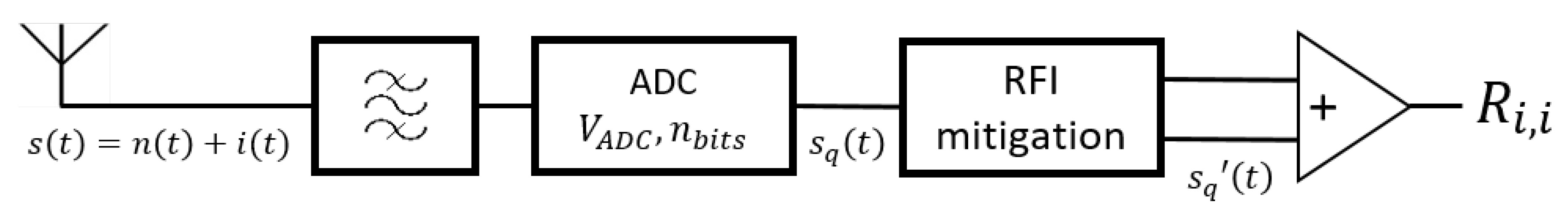
Considering the non-linearities of the quantization process and the broad number of RFI types and quantization schemes considered, analytical treatment of the problem is very problematic. Therefore, a simulated processing chain has been implemented mimicking the properties of a real system, including filtering, quantization, mitigation, and correlation. In Figure 1, the block diagram of the modules implemented is shown.
The contaminated signal has been simulated as a complex random noise source of 300 K, added to an RFI signal of varying type and power. The combined signal was sampled and filtered with an anti-aliasing filter of 27 MHz of bandwidth. This simulates the acquisition process of a generic digital radiometer. On a second stage, the combined signal is quantized with a generic quantizer with varying number of bits and a maximum . Finally, the resulting signal is RFI-mitigated by using several proven algorithms detailed below. Mitigation performance of these methods is compared to the performance in the non-quantized case, which has been computed too and is taken as the reference.
Ensembles of samples have been used. As shown in [29], sampling influences the computation of correlation. If low oversampling factors () are used, radiometric sensitivity is degraded. Therefore, to disregard this effect, an of 8 has been selected. Consequently, sampling frequency is , where is the output bandwidth of the anti-aliasing filter, 27 MHz.
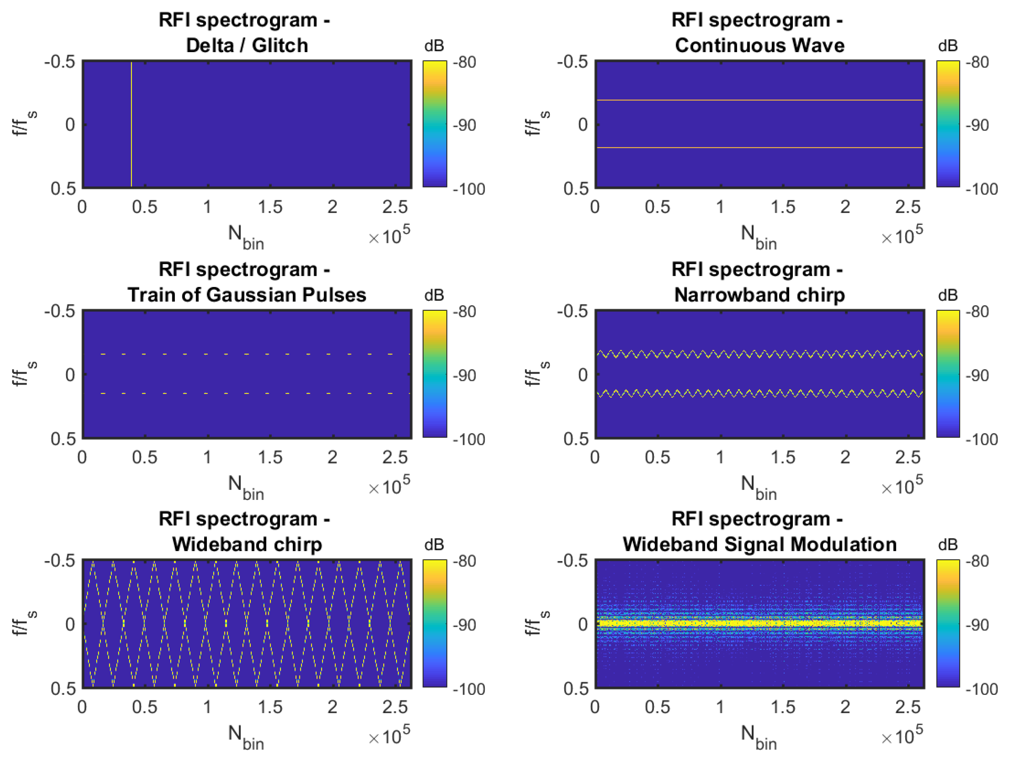
In the framework of this study, six different types of RFI have been simulated [36]:
- 1
- A delta function: A one-sample pulse simulating a very time-concentrated high-power signal captured by the antenna.
- 2
- A continuous wave (CW): A single tone signal (sinusoidal), simulating a narrowband modulation.
- 3
- A burst of pulses: a train of Gaussian pulses with a pulse repetition period () of samples, and a pulse width of samples.
- 4
- A narrowband chirp signal: A chirp signal sweeping linearly with a bandwidth of and a samples.
- 5
- A wideband chirp signal: A chirp signal sweeping linearly with a bandwidth of and a samples.
- 6
- A generic signal modulation: Simulated using a pseudo-random noise code (PRN) of , with its bandwidth overlapping the noise bandwidth.
These types are chosen as they are sufficiently representative of the most common types of RFI found. For example, pulsed signals are typical of Radar-originated RFIs, CW, or PRN are typical of narrow and wideband communication signals, etc. In Figure 2, their time/frequency signatures have been plotted. RFI power considered varies between 0 K and 15,000 K. Quantization is performed following several uniform quantization schemes: 1 bit, 2 bits, 3 bits, 4 bits, 5 bits, and 8 bits. All quantizers are mid-riser, where 0 is a decision threshold. Small, near-0 values are quantized as the first positive or negative level, depending on their sign.
For each of them, two representative ADC dynamic ranges () have been considered. In one case, , representing a system with a fixed adapted to the radiometric noise signal (being the standard deviation of the noise signal). As discussed, a system such as this is prone to clipping in the presence of RFI. On the other case, , being the standard deviation of the combined contaminated signal (noise + RFI). This corresponds to a system with an AGC system, designed to avoid clipping.
For the sake of simplicity, no quantization compression has been considered. As discussed previously, the use of compression actually degrades quantization noise with respect non-compressed quantizations in the presence of RFI. However, the combination of compression with large to avoid clipping could be a sensible compromise between the two methods above, and is proposed for future evaluation.
After quantization, mitigation is performed. Signals have been mitigated using 5 different Time/Frequency mitigation techniques:
PB and FB are performed digitally at the maximum available resolution, i.e., one sample. Therefore, PB time resolution is , and FB resolution is . Regarding SB, a balanced approach between frequency and time domains has been chosen, with equivalent resolutions for both. Taking into account the total number of samples N, the resolution for time is , and for frequency . Wavelet decomposition has been performed using Haar functions and a level of decomposition equal to .
These proven techniques have shown good results for selected RFI in the unquantized case [36]. They are based on the detection of concentrations of energy in certain transformed domains (such as the Time/Frequency domain). Natural radiometric sources produce ’white’ signals without any concentration of energy in the transformed domains. Therefore, any concentration is regarded as RFI-induced. It is important to remark that this family of techniques does not assume anything on the RFI type or power. In addition, it should be noted that these techniques work better for some RFI than for others. Therefore, the final selection depends on the specific RFI environment that the instrument will face. MFTB provides a reasonable trade-off if nothing can be assumed about the type of RFI encountered [36].
The removal of this energy produces an RFI-free signal, and is performed by comparison with a decision power threshold . This threshold must be computed from an RFI-free calibration signal, and it is closely related to the probability of false alarm [40]:
where is the variance of the RFI-free noise calibration signal. In this work, has been set to . Thanks to the useful properties of Gaussian white noise, in a Total Power Radiometer this threshold value may be computed in the temporal domain and applied in any Fourier-like transformed domain [36]. However, in a digital or correlation radiometer, the need for an aliasing filtering and oversampling makes the radiometric noise colored (i.e., non-white). Consequently, the threshold must be computed in each transformed domain. This has been done by estimating a local variance , where z stands for the domain’s variable into consideration.
Since the probability of false alarm is not 0, even in an RFI-free scenario the use of any RFI mitigation algorithm implies that some RFI-free samples will be discarded. This loss of energy must be compensated for. In this study, and considering the spectral response of the filtered noise, this correction has been estimated by computing:
where is the power of the RFI-free calibration noise signal, and is the power of this signal after mitigation. Then, , where is the power of the RFI-contaminated signal after mitigation. The goodness of the estimator depends directly on both the and the number of samples. With higher more samples are required to provide a good estimation. This correction has been applied to all results in Section 3. As it will be shown, with a fixed and samples, the estimation is good enough so that the final bias <1 K. It should be made clear that this loss of energy induced by RFI mitigation methods in RFI-free conditions has nothing to do with the loss of energy induced by clipping, discussed later in this paper.
After mitigation, the autocorrelation is computed. Only the case where the two branches of the correlation have been quantized identically has been considered. To denormalize the quantized correlation, the denormalization function is computed following [29]. The retrieved power is then computed as the value at the origin of this autocorrelation function, . The shape of the autocorrelation is also analyzed.
RFI mitigation performance is measured by the delta between the resulting power after mitigation, , and the original noise temperature without RFI (300 K). Residual RFI temperature, , may be positive in case that the mitigation does not completely remove the RFI. However, when mitigating quantized signals, this residual may be negative. This means that the resulting signal after mitigation has lower power than the original noise signal, and accounts for the fact that the presence of RFI and quantization has destroyed most of the original radiometric signal.
3. Results
3.1. Fixed VADC
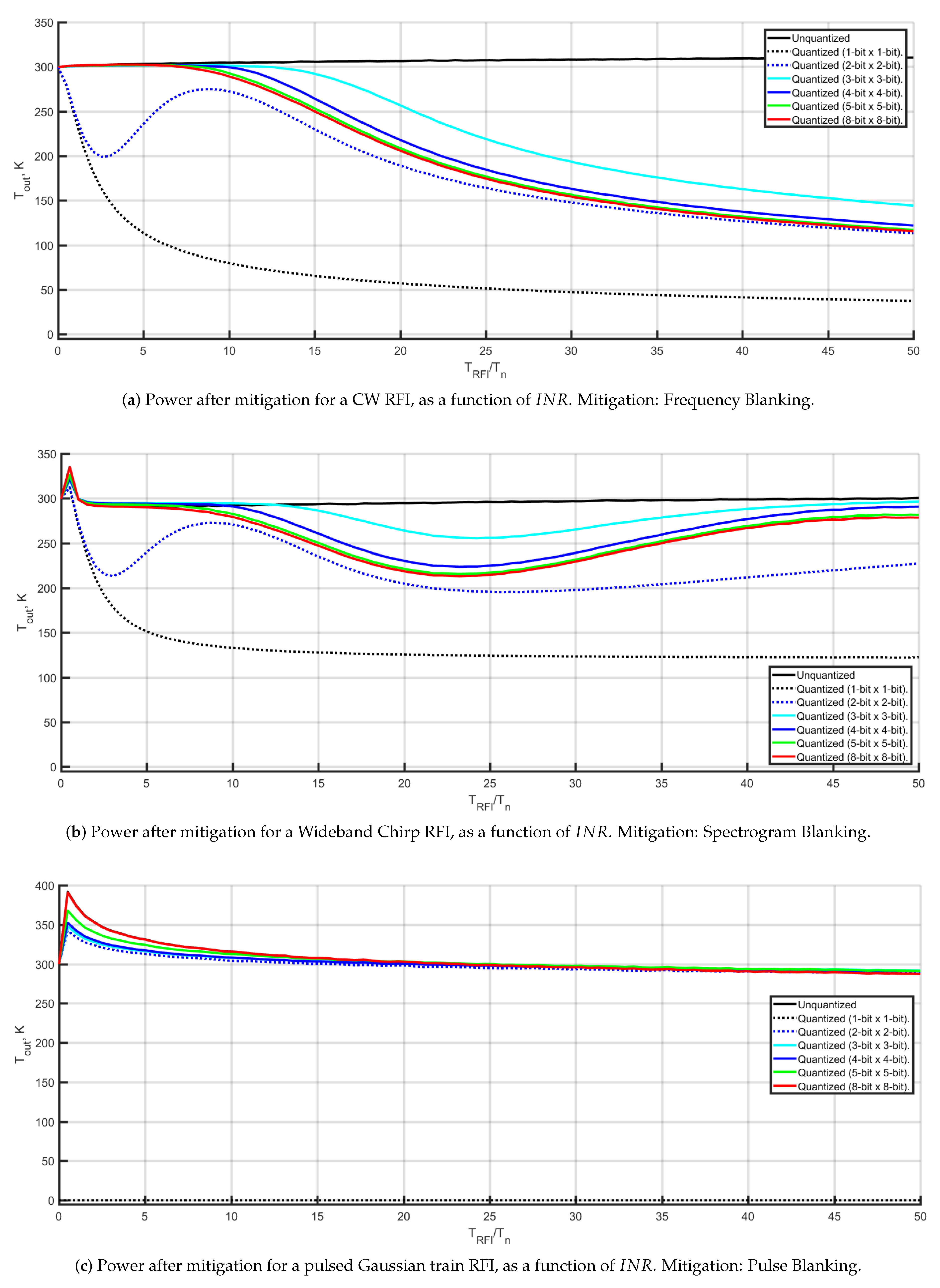
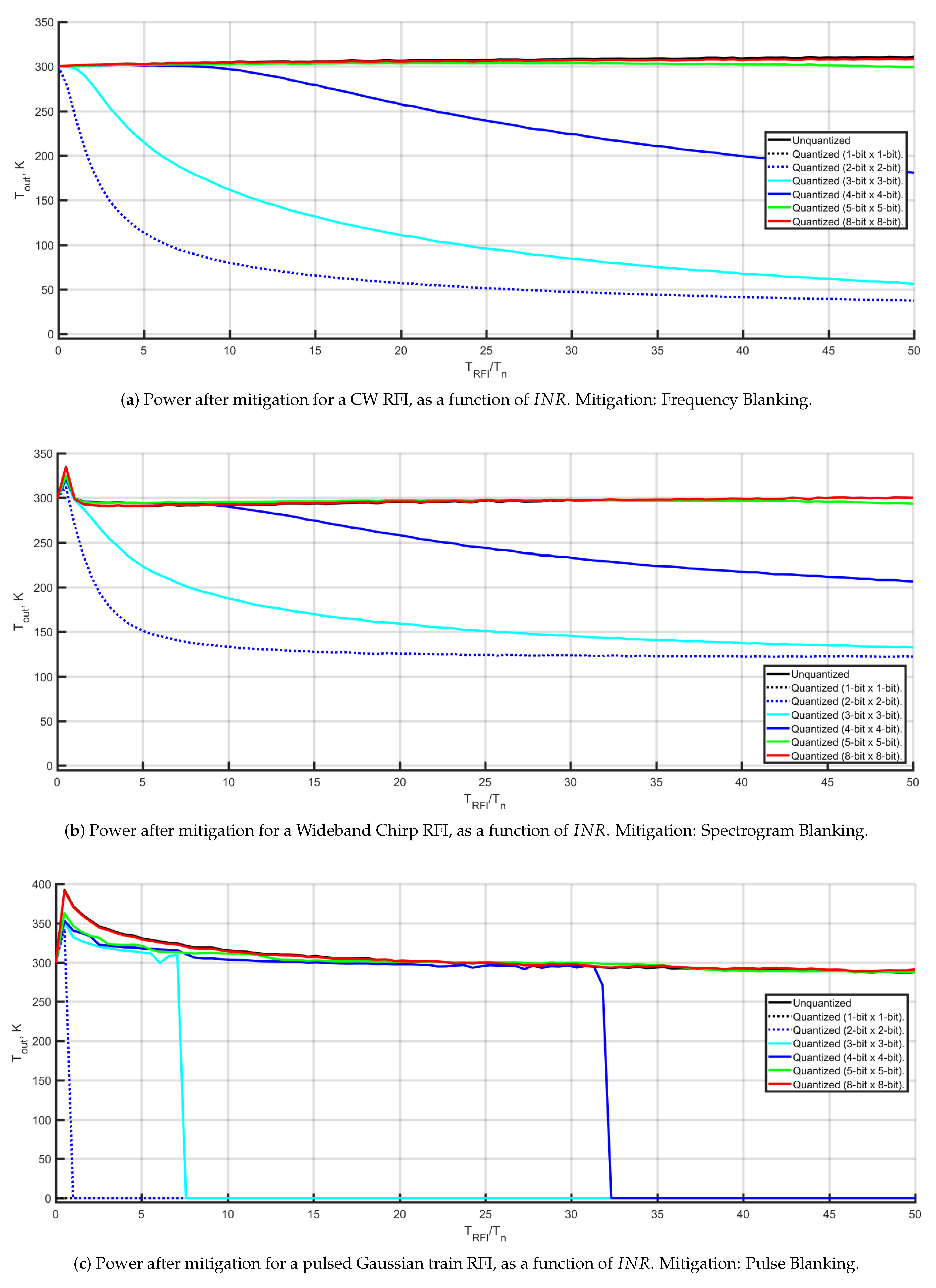
A fixed dynamic range, , accounts for a system where has been tailored to represent well the expected noise signal, but that will clip easily if RFI is introduced. Let us examine the effects of said configuration on mitigated retrieved power. In Figure 3, the retrieved power is plotted as a function of the interference-to-noise ratio, (note that it has been plotted in linear units), for several RFI type/mitigation pairs considered. Pairing of RFI types and mitigation techniques has been selected taking the most appropriate technique for each type, following [36]. Quantized mitigation performance should be compared with the performance of the unquantized case.
- Frequency Blanking shows very good performance when mitigating CW signals for the unquantized case. If quantized signals are considered, the performances are comparable to the reference if the clipping induced by the RFI is relatively small (). If clipping appears, performance quickly degrades for any quantization method, making mitigation of large power RFI not possible. Performance is comparable for non-coarse-quantization schemes (3–8 bits), as the drop-out happens for a similar . Therefore, in this configuration, a higher number of bits does not offer any advantage in what concerns RFI mitigation. This is compatible with the fact that the limiting factor is clipping, which depends on , regardless of bit density. Although not included for simplicity, narrowband chirp RFI mitigated with FB exhibits very similar behavior for all quantization schemes. 1-bit and 2-bit quantization do not provide good performance regardless of , even for small RFI powers. This is because 1-bit and 2-bit are, by definition, introducing clipping regardless of RFI power. 2-bit quantization, however, exhibits an apparent recovery for . The reason for this is still to be understood but, as it will be shown, even if the power performance seems to recover, Gaussianity of the signal is strongly affected.
- Spectrogram Blanking shows a similar behavior than FB. Performance also exhibits drop-outs originated by clipping, and they appear for similar . However, for high RFI powers (), performance seems to recover. This, however, is related to non-mitigated residuals that for high , are noticeable. In such a case, the statistics of the signal would not be Gaussian, and the correlation would not be sinc-shaped. It should be noted that SB is not able to detect well the RFI when the power is comparable to the noise (). This happens too for the unquantized case, and therefore is not originated by the digitization process. This effect is related to the resolution of some of the techniques [36], the T/F properties of the RFI, remaining residuals, etc., and it is observed too for PB, WB, and MFTB.
- Pulse Blanking shows very good performance for all quantization schemes, without drop-outs attributable to clipping. This is related to how PB works. Indeed, for any quantization scheme with more than 2 quantization levels (i.e., 1-bit), the power decision threshold can be tailored to discriminate pulsed RFI. Equivalently, due to the nature of this mitigation, 1-bit quantization cannot work at all: as the decision power threshold is applied in time, and the signal power in time is constant, there are two possibilities (depending on ): or the entire ensemble is discarded, or no sample is flagged as RFI. As the nature of the RFI is comparable, very similar performances are obtained if delta RFI is mitigated with PB.
- Wavelet Blanking performance is comparable to FB and SB, but mitigation is possible for a slightly higher range (). As with FB, performance degrades for higher , and coarse quantization does not work for any considered.
- Multi-resolution Fourier Transform Blanking performance for the unquantized case is not comparable to the ones shown by the other methods. Indeed, for moderate , the method over-corrects, and some residuals are left for higher . Nevertheless, it should be noted that MFTB is a generalist method not tailored to any particular RFI type. Therefore, worse performance with respect the rest of the pairs is expected. Regardless of its absolute performance, the impact of quantization is comparable to the rest of methods: for , the quantized signatures depart from the unquantized mitigation, and this is attributable to signal clipping.
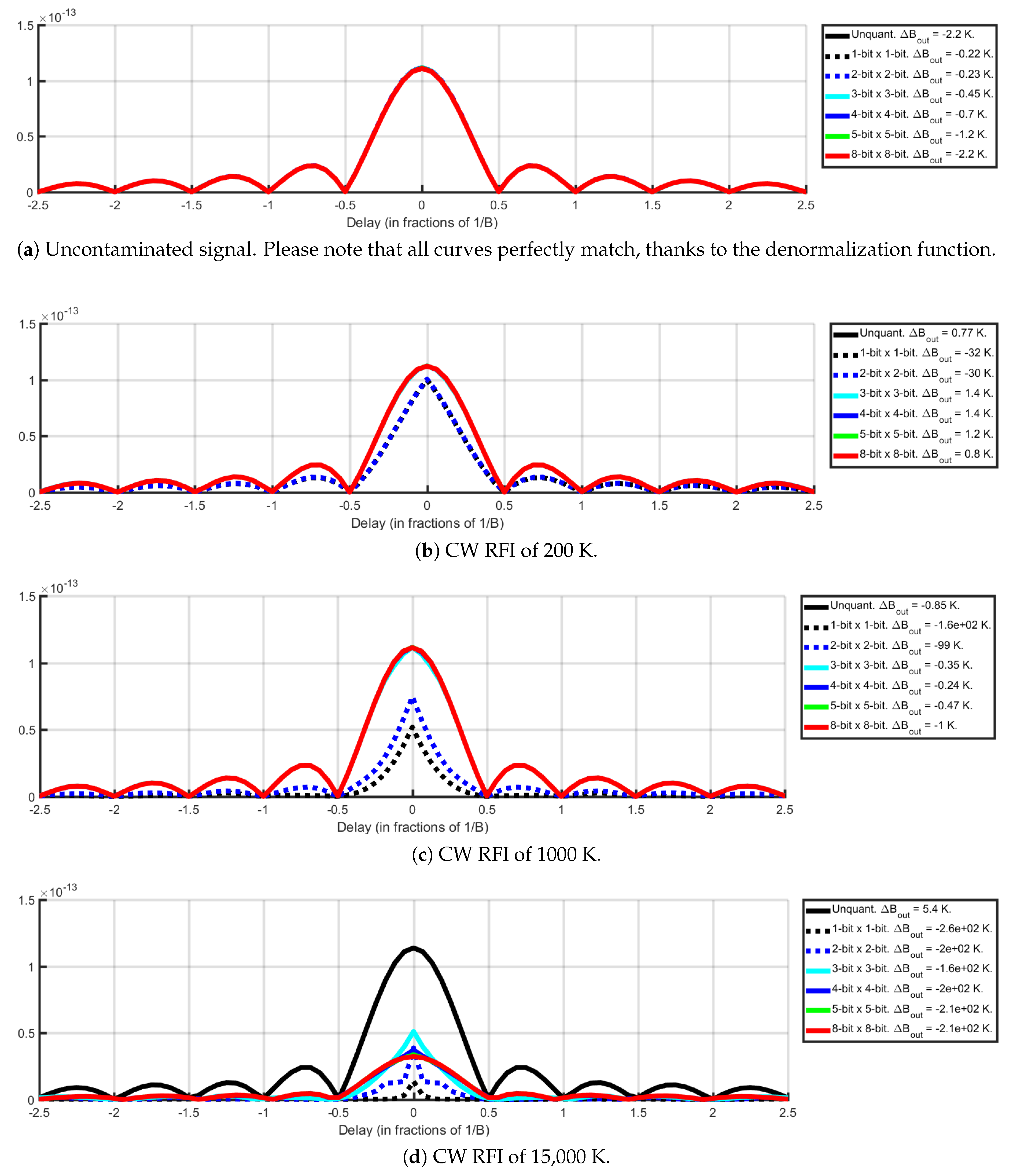
Let us examine the effects on correlation shape for some relevant cases. In Figure 4, the autocorrelation results for a CW-contaminated signal mitigated with Frequency Blanking (FB) are shown. The autocorrelation curves obtained for different quantization schemes are presented. It can be seen that in the absence of RFI (Figure 4a), FB behaves consistently, and the debiasing factor is well estimated for all quantization schemes. Additionally, it can be seen that denormalization of the autocorrelation works as expected, as all autocorrelations match perfectly in the RFI-free case. In Figure 4b–d, it can be seen that FB works well in the unquantized case for all temperatures considered, with residuals below 1% of the input RFI temperature. However, if quantization is introduced, performance degrades very quickly. While, for RFI of moderate power (200 and 1000 K), FB works reasonably well if a large number of bits is used, its performance degrades for larger RFI. FB fails in all quantized cases when mitigating high power (15,000 K) RFI, due to the large portion of the energy that has been clipped. In addition, coarse-quantization schemes such as 1-bit do not work regardless of RFI power.
It is interesting to note the relationship between autocorrelation shape and Gaussianity of the mitigated signal. In fact, a sinc-shaped autocorrelation is indicative of the fact that the mitigated signal follows a Gaussian distribution. This can be seen in Figure 4d: for 8-bit quantization, and even if clipping prevents a proper retrieval of the original signal power, mitigation has been able to generate a signal of approximate Gaussian statistics. Therefore, the resulting shape after denormalization is sinc-shaped. However, for other quantization cases (e.g., 1-bit), the resulting shape is not sinc-shaped, revealing that mitigation has not been able to produce a Gaussian signal. This may be true even if the power performance apparently recovers (e.g., 2-bit quantization for ).
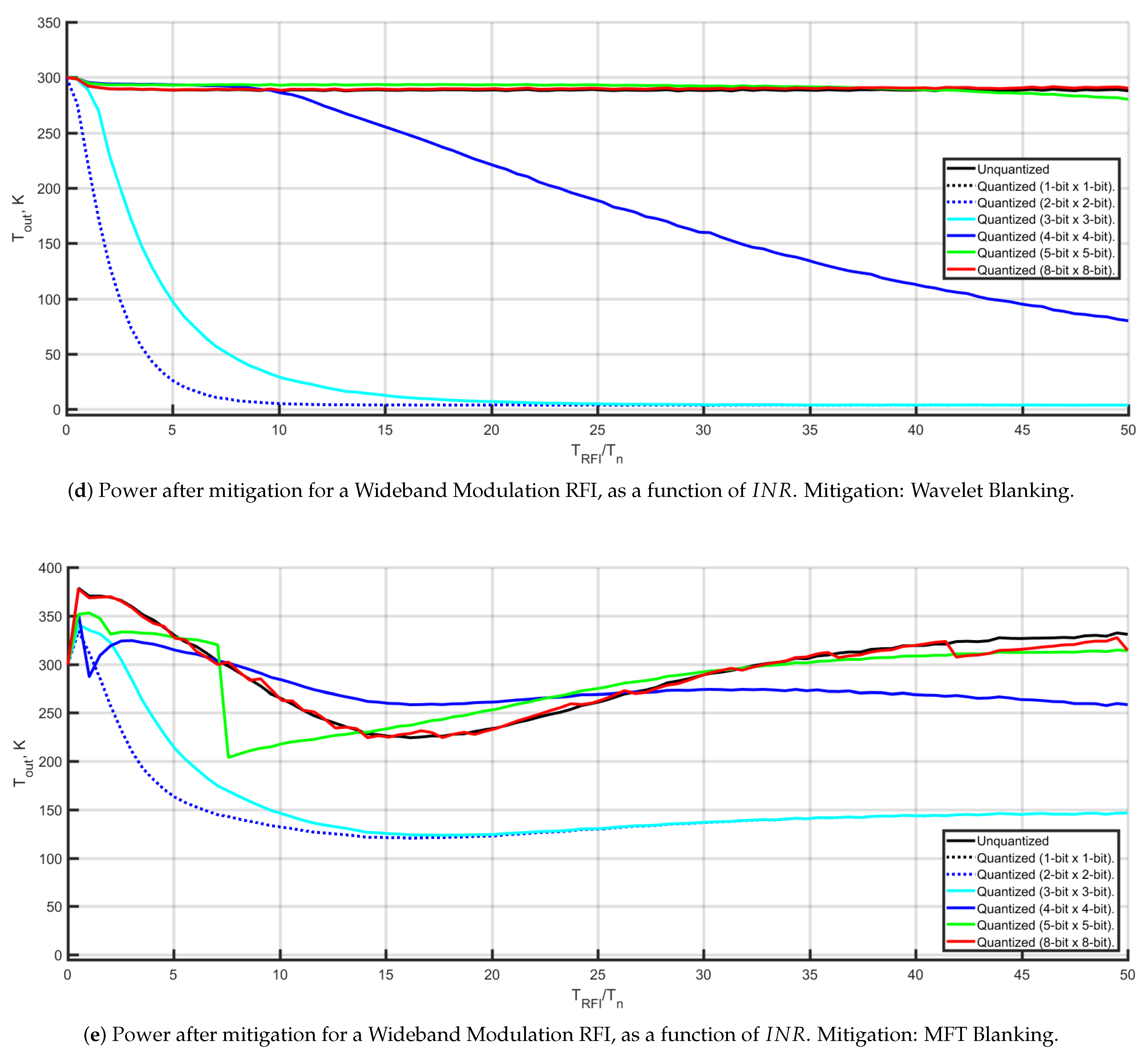
3.2. Adaptive
In this section, a system with Automatic Gain Control, designed to avoid clipping, is considered. Therefore, . In Figure 5, the output power is plotted as a function of the . This figure is equivalent to Figure 3, with the only change of the dynamic range. Consequently, the behavior of the reference does not change.
- Frequency Blanking shows some differences with respect fixed . In particular, 5 and 8-bit quantizers present performances comparable to the reference for high . Therefore, mitigation of high-power RFI is feasible with dense quantizers if AGC is implemented. However, 3 and 4-bit quantizers exhibit quick drops of performance at and respectively. While 4-bit performance is similar to respect fixed , 3-bit quantizer clearly degrades. The origin for these drops of performance has been called ‘underquantization’, and is related to the inability of the quantization to represent properly the statistics of the radiometric signal. ‘Underquantization’, in fact, impacts all quantizers, even 5 or 8-bit. In this case, however, it only comes into play for very high RFI powers (i.e., ), not covered in this study. This effect is briefly described in the next section.
- Spectrogram Blanking and Wavelet Blanking exhibit very similar results, with 5 and 8-bit quantizers showing good performance for larger RFI, and 3 and 4-bit quantizers featuring drops. Coarse quantization (1 and 2-bits) shows very bad performances overall for the three methods.
- Multi-resolution Fourier Transform Blanking exhibits also comparable results. For 5-bit quantization, however, it shows sudden drops of performance. This may be linked to instabilities on the denormalization process, but it is unclear why this effect does not appear for other quantization schemes.
- Pulse Blanking shows worst results with AGC. Indeed, the performance drops for 3 and 4-bits were not present without AGC. The ‘sharpness’ of the drops is related to how the power decision threshold is set: eventually, all samples are flagged as RFI-contaminated. As high-power RFI can be mitigated without the need for adaptive , the use of AGC for PB is not recommended.
Therefore, AGC is a viable solution to mitigate high-power RFI, provided that dense quantizers () are available. 5-bits quantization presents a very wide margin of operation, showing good performance up to an of 50. Systems with a larger number of bits increase even further this margin of operation. The selection of the minimum number of bits that are necessary depends, thus, on the expected RFI environment. If system complexity is an issue, then a 3-bit quantizer with fixed would suffice for .
It should be remarked that 1-bit and 2-bit quantization curves perfectly match in all cases considered, exhibiting very poor performances regardless of . This is caused by the inherent signal clipping introduced in both cases. It is interesting, however, to analyze why the introduction of AGC makes 1-bit and 2-bit essentially identical. By using AGC, is especially tailored to guarantee that the quantizer does not clip the signal. Consequently, higher decision levels are very rarely reached. While this is of no major consequence for a larger number of bits, 2-bit quantizer only has 4 quantization levels. Therefore, as only the 2 lower levels are used, 2-bit acts effectively as a 1-bit quantizer.
In Figure 6, the autocorrelation results for a CW-contaminated signal mitigated with Frequency Blanking (FB) and AGC are shown. For non-coarse-quantization, autocorrelation shapes match the reference if the quantization can represent properly the radiometric noise. When this is no longer true, shape departs from the expected sinc. It is worth remarking how Gaussianity is lost before the performance starts degrading. Indeed, for an RFI power of 15,000 K, power performance of 5-bit quantizer is still not strongly affected by underquantization (see Figure 5a, for ). However, when the shape is examined (Figure 6d), it is clear how the statistics are already affected, even if the residuals are still below 1% of the input RFI temperature.
4. Discussion
To support the interpretation of the simulation results provided, a more formal study of the effects of quantization is given in this section. As discussed, quantization is a non-linear operation which is difficult to treat mathematically. However, quantization may be understood as an amplitude sampling of the signal. As signals are usually stochastic processes, they are defined statistically by their Probability Density Functions (PDFs). Quantization, then, can be described as an operator on its statistical amplitude described by the PDF. This approach was followed by Widrow et al. to derive a statistical theory of quantization [41,42,43], where some parallelisms between the sampling theorems and the quantization were found. However, the specifics of clipping were not discussed, as Widrow’s work focused mainly on quantization noise.
4.1. Clipping Impact to RFI Mitigation
To understand the effects of clipping, let us consider a system with a sufficiently large number of bits, but a finite . Hence, quantization noise can be neglected, and it is worth analyzing how clipping alone distorts the statistical and time-frequency properties of a radiometric signal contaminated by RFI.
Let’s consider a signal defined as , where is a Gaussian radiometric signal of power , and is a generic RFI signal with power . Being a zero-mean Gaussian random variable, its PDF is defined by [44] (pp. 361–362):
with being the standard deviation of the noise. For simplicity, and have been chosen to be real, but for band-pass signals, they must be complex. On the other hand, the PDF of is generic and noted as . Then, the PDF of can be computed by convolving:
Taking into account that the Characteristic Functions and are the Fourier transforms of their respective PDFs, such convolution may be computed as a product of in the frequency domain. Now, let us consider a system that fully clips any input value , while accurately mimicking the original signal otherwise. This would be the response of an ideal quantization scheme of finite dynamic range and infinite number of bits. In this conditions, the quantized signal’s PDF, is:
which could be expressed in a more compact form using the sampling property of the Dirac delta and the rectangular function:
where and . Therefore, clipping concentrates part of the probability of the original PDF on . Assuming a zero-mean , is symmetric, , and variance of this clipped signal is:
From the above expression, it is evident that the variance of the clipped signal will be lower than the variance of the unclipped signal. Clipping, therefore, introduces an unavoidable loss of energy, :
This loss of energy cannot be recovered by any mitigation algorithm. As explained before, time/frequency mitigation algorithms are based on the detection and removal of concentrations of energy. If the combined signal has been clipped, its power will be lower than the combined signal without clipping.
Clipping is a non-linear operation, this loss of energy cannot be split between separable contributions depending on RFI and on radiometric signal: it affects to the non-separable combined signal. In the most extreme case (i.e., full clipping), signal power will be driven solely by :
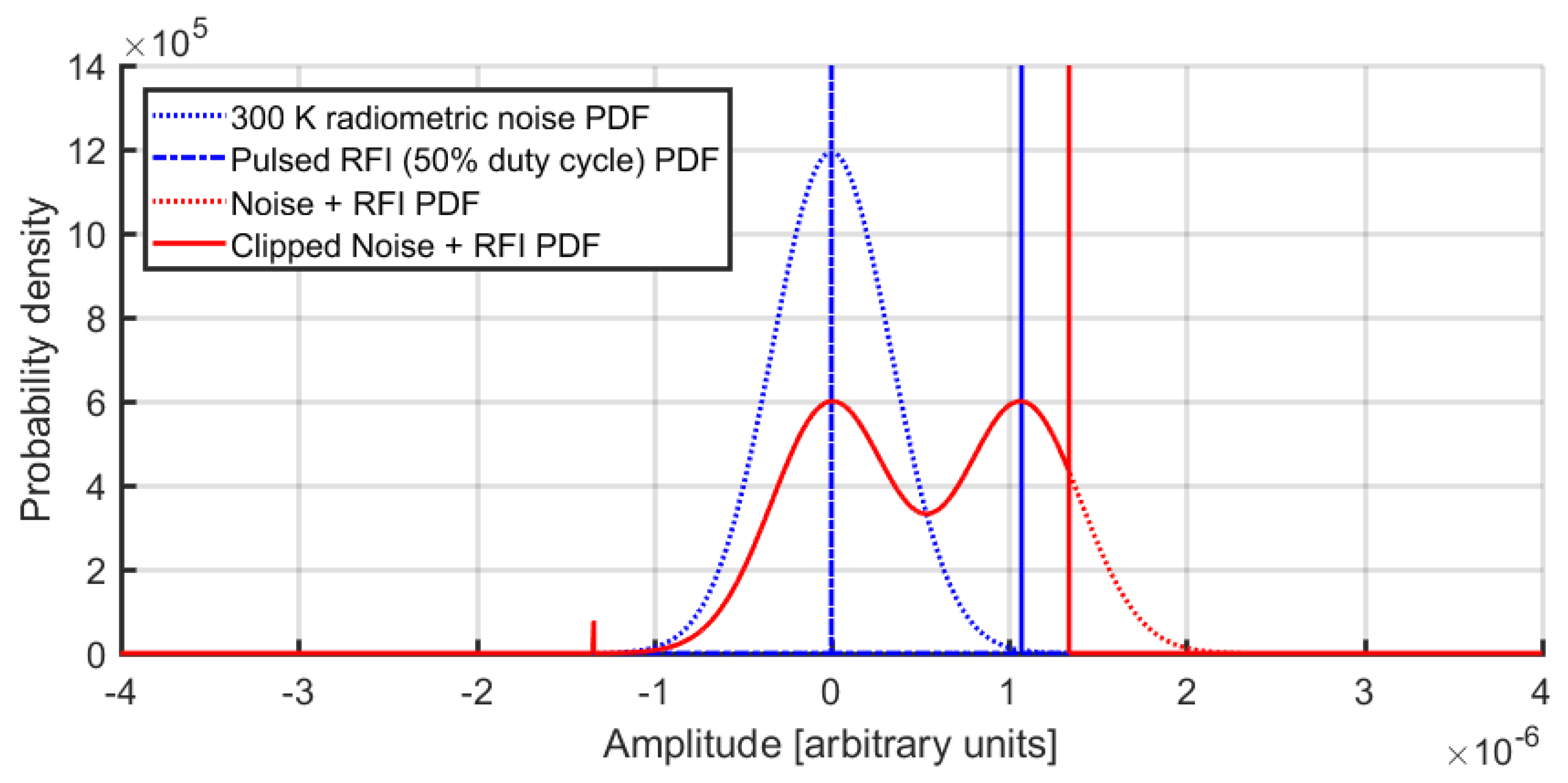
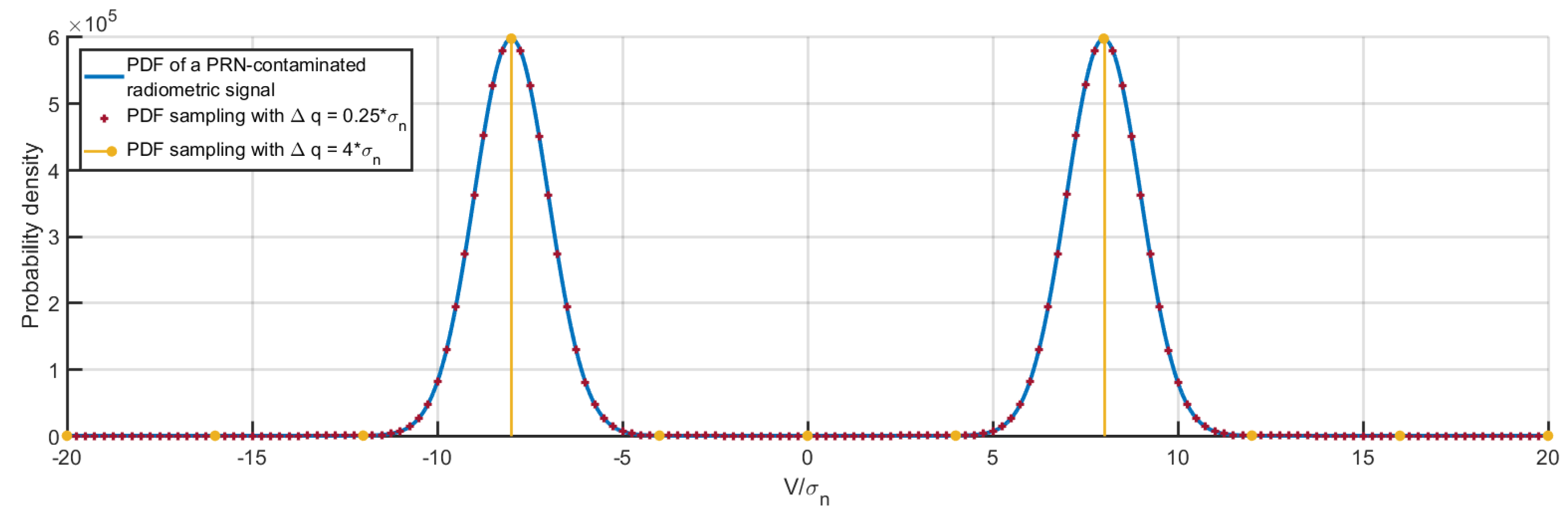
Let’s consider, as an example, the RFI defined by:
This PDF is representative of a radar-originated, pulsed RFI of of amplitude and a duty cycle of . From Equations (4) and (5), then the PDF of the combined signal will be:
The associated PDF for this type of RFI is plotted in Figure 7. As it can be readily seen, clipped power depends strongly on the PDF shape of the RFI, which in this case depends on RFI type and duty cycle. As in general the statistics of the RFI are unknown, there is no way to determine the amount of power clipped, and therefore the measured power cannot be compensated for this.
In addition to this loss of energy, clipping also changes fundamentally the time-frequency properties of the signal. Clipping is, by definition, a sharp transition in time, resulting in a spreading of the signal bandwidth in frequency. The clipping effects on the spectrum of a band-limited noise signal were studied in detail in the early Van Vleck’s and Middleton study [35]. In the absence of RFI, clipping originates a spreading of the band-limited noise outside of the passband. This is too the effect of 1-bit quantization over Gaussian noise, as this quantization scheme could be understood as a system that fully clips the input power.
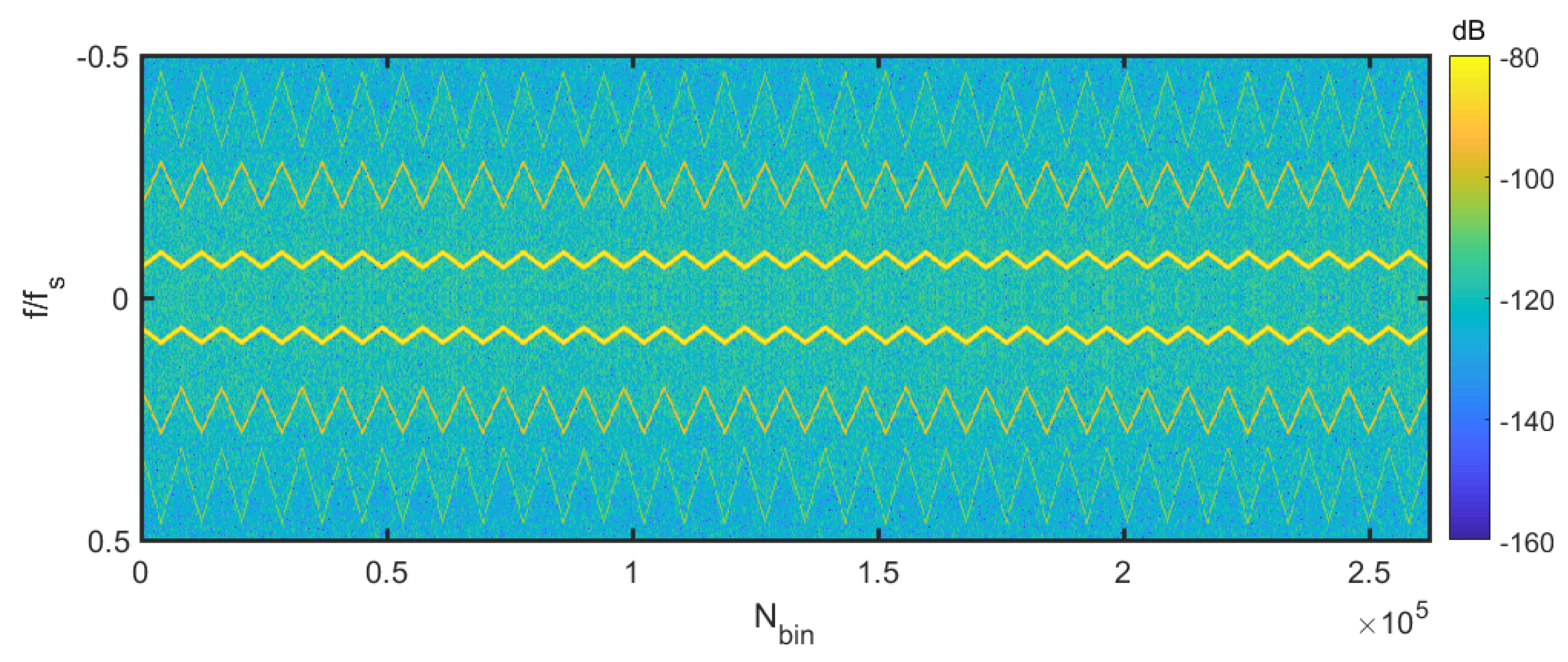
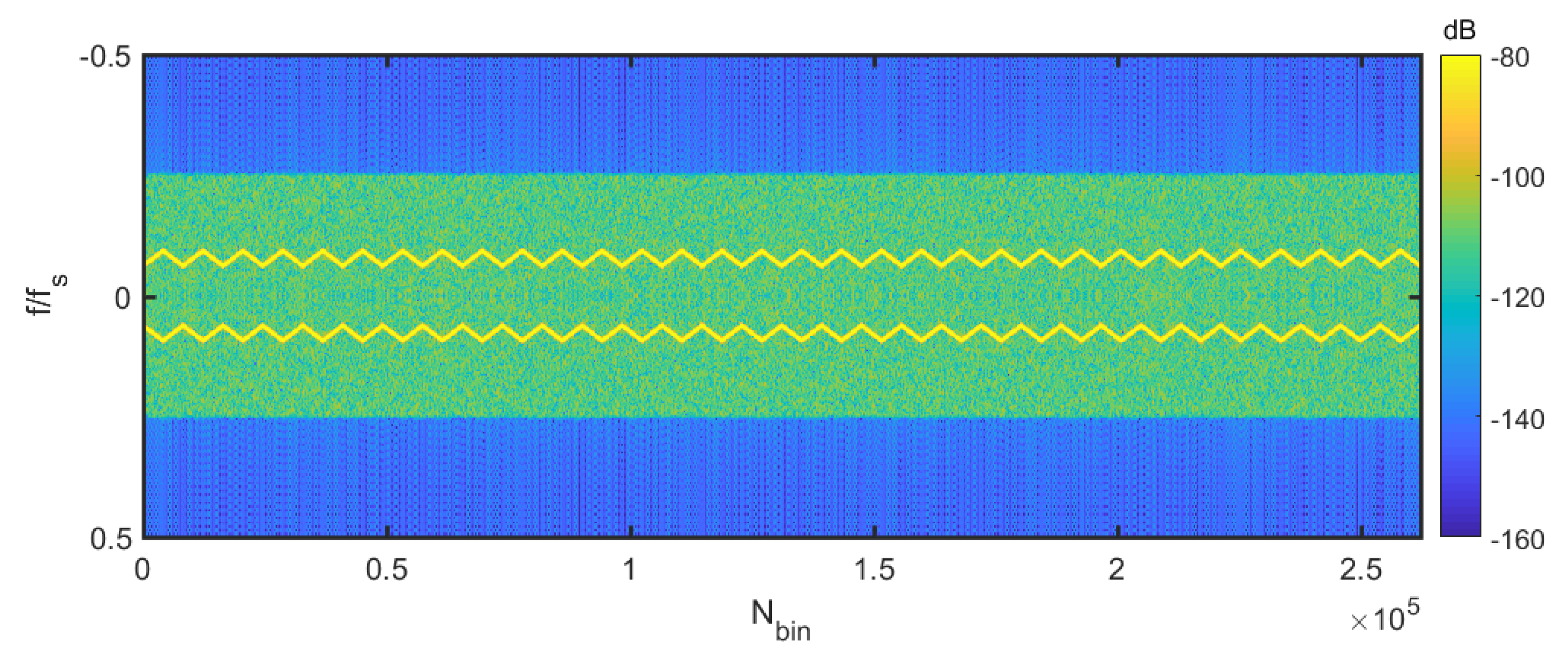
Qualitatively, if the RFI appears concentrated in frequency (e.g., a CW), clipping originates harmonics at multiples of the RFI fundamental frequency. The spectral width of those harmonics increases proportionally to the harmonic number. Therefore, the RFI is spread in frequency, contaminating a larger fraction of the signal’s bandwidth. In addition, as the signal is no longer band-limited, high-order harmonics enter the passband as aliases. These effects can be appreciated in Figure 8, where the spectrogram of a clipped noise signal contaminated by a chirp RFI of 15,000 K is shown. To force strong signal clipping, has been set to , with a power temperature for the noise of 300 K. For comparison, the same unclipped signal is plotted in Figure 9.
4.2. The ‘Underquantization’ Problem
Let us consider now the second scenario, i.e., a system with a fixed number of bits and a variable . As a suitable convention to keep clipping under acceptable levels, . In this case, and assuming b bits, the quantization step will be:
By design, the quantization step depends on the power of the combined signal. Consequently, larger will result in larger . While is somewhat limited in Earth Observation applications, is not, and therefore, the quantization step considered may be arbitrarily high. To study this, let us base our analysis in Widrow’s et al statistical quantization theory [41]. Widrow’s work states that if the PDF of the signal is band-limited (i.e., their CF is limited in frequency) so that for , then the original PDF can be reconstructed from the PDF of the quantized signal. Equivalently, quantization can represent properly the statistics of the signal.
Let us consider the problem of quantization of an RFI-free noise signal. Gaussian signals are never strictly band-limited. In fact, their is Gaussian too, with standard deviation . However, most of its energy (more than 99%) falls below from its center. Therefore, its PDF may be considered to be band-limited with bandwidth . As a consequence, the original PDF could be (approximatively) recovered from the quantized PDF as long as Widrow’s first condition applies, i.e., . Or equivalently,
This is based on the fact that quantization is similar to sampling the PDF. Sampling the PDF would introduce replicas every on the frequency/ domain. If Equation (14) verifies, then these replicas do not overlap. Taking the central replica (or, in the probability domain, interpolating the PDF) makes possible the complete recovery of the original PDF [41] (pp. 353–354).
Let us consider now a signal contaminated by the RFI defined by Equation (15), an equiprobable PRN:
The PDF of the combined signal is shown in Figure 10 (blue line). In that case, is the product of and :
That is, a cosine damped by the Gaussian function. Consequently, is as band-limited as , and the same considerations apply. Therefore, if Equation (14) holds, taking the fundamental replica will yield:
with being Widrow’s area sampling function [41].
However, as stated in Equation (13), will increase if grows. Consequently, Equation (14) will eventually not be fulfilled, meaning that high-order replicas overlap with the fundamental replica (i.e., aliasing appears). After quantization, becomes the sum of all its aliases:
Now, if the fundamental replica contaminated by aliases is taken:
In general, this makes , and by extension the PDF, non-recoverable. If the question is examined in the PDF domain, something equivalent happens. It is easy to see that if the quantization step is very large with respect to the width of the Gaussian PDF, then quantization is not sampling properly the shape of , only the PDF of the interference. Therefore, the quantized signal does not contain any radiometric information. In Figure 10, the resulting PDF of two different quantizations on the PDF are compared. As it can be readily seen, quantization with large removes any information attributable to radiometric noise. Indeed, the coarseness of this quantization is unable to represent faithfully the Gaussian shape of the radiometric signal, and the resulting PDF only contains RFI information (i.e., two deltas for a PRN RFI). Hence large RFI power leads to large and large , which in turn will lead to undersampling of the radiometric noise information.
It is worth noting that the impact of this effect is directly dependent on the number of bits considered. The larger the number of bits, the lower the impact. Indeed, for the same , is lower with a higher number of bits, and this effect will appear for larger .
5. Conclusions
In this work, the influence of quantization on RFI mitigation performance has been analyzed for different types of RFI as a function of the gain control (either constant or adaptive) and interference-to-noise ratio.
It has been demonstrated that clipping prevents the optimum performance of mitigation algorithms, because the energy content of the signal is strongly affected. This impairs the usefulness of RFI mitigation for large RFI powers. Pulse Blanking is the exception to this, showing performances comparable to the unquantized case, even for high . The rest of mitigation algorithms, however, are only able to correct RFI up to an of 6–10. Depending on the expected RFI environment, this could be insufficient. Therefore, clipping must be avoided as much as possible.
Automatic Gain Control systems adapt the input signal to the dynamic range of the quantizer, preventing clipping, and therefore allowing RFI mitigation. However, because of the finite number of bits and the quantization step, as RFI power increases, the quantization step increases too. Eventually, the quantization is not able to properly reproduce the radiometric signal, but only the RFI, and the mitigation performance degrades. This effect, that it has been termed as signal ‘underquantization’, depends strongly on the number of bits considered. Therefore, a trade-off exists between system complexity and operation range of the RFI mitigation algorithms. ‘Underquantization’, however, degrades performance with respect fixed for 3 and 4-bits quantizers.
In addition, it has been demonstrated that 1-bit quantization prevents the use of any time/frequency mitigation method, regardless of RFI power or other system parameters. This is due to the clipping effects inherent to these coarse-quantization schemes, which are not avoidable using AGC systems.
Author Contributions
Conceptualization and methodology, R.D.-G. and A.C.; software and validation, R.D.-G.; formal analysis and investigation, R.D.-G.; writing—original draft preparation, R.D.-G.; writing—review and editing, A.C.; supervision, A.C.
Funding
This project has been supported by projects MDM-2016-0600, and EU ERDF project RTI2018-099008-B-C21 “Sensing with pioneering opportunistic techniques” of the Spanish Ministerio de Ciencia, Innovación y Universidades.
Conflicts of Interest
The authors declare no conflict of interest. The funders had no role in the design of the study; in the collection, analyses, or interpretation of data; in the writing of the manuscript, or in the decision to publish the results.
References
- National Research Council. Spectrum Management for Science in the 21st Century; The National Academies Press: Washington, DC, USA, 2010. [Google Scholar]
- Draper, D.; Newell, D. An assessment of radio frequency interference using the GPM Microwave Imager. In Proceedings of the 2015 IEEE International Geoscience and Remote Sensing Symposium (IGARSS), Milan, Italy, 26–31 July 2015; pp. 5170–5173. [Google Scholar]
- Misra, S.; de Matthaeis, P. Passive Remote Sensing and Radio Frequency Interference (RFI): An Overview of Spectrum Allocations and RFI Management Algorithms. IEEE Geosci. Remote Sens. Mag. 2014, 2, 68–73. [Google Scholar] [CrossRef]
- Misra, S.; Mohammed, P.N.; Guner, B.; Ruf, C.S.; Piepmeier, J.R.; Johnson, J.T. Microwave radiometer radio-frequency interference detection algorithms: A comparative study. IEEE Trans. Geosci. Remote Sens. 2009, 47, 3742–3754. [Google Scholar] [CrossRef]
- Anderson, T.W.; Darling, D.A. A test of goodness of fit. J. Am. Stat. Assoc. 1954, 49, 765–769. [Google Scholar] [CrossRef]
- Jarque, C.M.; Bera, A.K. A test for normality of observations and regression residuals. Int. Stat. Rev. Revue Int. Stat. 1987, 55, 163–172. [Google Scholar] [CrossRef]
- D’Agostino, R.B.; Belanger, A.; D’Agostino, R.B., Jr. A suggestion for using powerful and informative tests of normality. Am. Stat. 1990, 44, 316–321. [Google Scholar]
- Lilliefors, H.W. On the Kolmogorov-Smirnov test for normality with mean and variance unknown. J. Am. Stat. Assoc. 1967, 62, 399–402. [Google Scholar] [CrossRef]
- Shapiro, S.S.; Wilk, M.B. An analysis of variance test for normality (complete samples). Biometrika 1965, 52, 591–611. [Google Scholar] [CrossRef]
- Lin, C.; Mudholkar, G.S. A simple test for normality against asymmetric alternatives. Biometrika 1980, 67, 455–461. [Google Scholar] [CrossRef]
- Kristensen, S.S.; Balling, J.; Skou, N.; Søbjœrg, S.S. RFI in SMOS data detected by polarimetry. In Proceedings of the 2012 IEEE International Geoscience and Remote Sensing Symposium, Munich, Germany, 22–27 July 2012; pp. 3320–3323. [Google Scholar]
- Camps, A.; Gourrion, J.; Tarongi, J.M.; Vall Llossera, M.; Gutierrez, A.; Barbosa, J.; Castro, R. Radio-frequency interference detection and mitigation algorithms for synthetic aperture radiometers. Algorithms 2011, 4, 155–182. [Google Scholar] [CrossRef]
- Park, H.; González-Gambau, V.; Camps, A.; Vall-Llossera, M. Improved MUSIC-based SMOS RFI source detection and geolocation algorithm. IEEE Trans. Geosci. Remote Sens. 2015, 54, 1311–1322. [Google Scholar] [CrossRef]
- Oliva, R. Mitigation of SMOS RFI Contamination Based on BT Frequency Extrapolation. In Proceedings of the IGARSS 2018—2018 IEEE International Geoscience and Remote Sensing Symposium, Valencia, Spain, 22–27 July 2018; pp. 309–312. [Google Scholar]
- Ellingson, S.W.; Bunton, J.D.; Bell, J.F. Removal of the GLONASS C/A signal from OH spectral line observations using a parametric modeling technique. Astrophys. J. Suppl. Ser. 2001, 135, 87. [Google Scholar] [CrossRef]
- Niamsuwan, N.; Johnson, J.T.; Ellingson, S.W. Examination of a simple pulse-blanking technique for radio frequency interference mitigation. Radio Sci. 2005, 40, 1–11. [Google Scholar] [CrossRef]
- Bradley, D.; Brambora, C.; Wong, M.E.; Miles, L.; Durachka, D.; Farmer, B.; Mohammed, P.; Piepmier, J.; Medeiros, J.; Martin, N.; et al. Radio-frequency interference (RFI) mitigation for the soil moisture active/passive (SMAP) radiometer. In Proceedings of the 2010 IEEE International Geoscience and Remote Sensing Symposium, Honolulu, HI, USA, 25–30 July 2010; pp. 2015–2018. [Google Scholar]
- Tarongi, J.M.; Camps, A. Radio frequency interference detection and mitigation algorithms based on spectrogram analysis. Algorithms 2011, 4, 239–261. [Google Scholar] [CrossRef]
- Querol, J. Radio Frequency Interference Detection and Mitigation Techniques for Navigation and Earth Observation. Ph.D. Thesis, Universitat Politècnica de Catalunya, Barcelona, Spain, 2018. [Google Scholar]
- Misra, S.; Kocz, J.; Jarnot, R.; Brown, S.T.; Bendig, R.; Felten, C.; Johnson, J.T. Development of an On-Board Wide-Band Processor for Radio Frequency Interference Detection and Filtering. IEEE Trans. Geosci. Remote Sens. 2018, 57, 3191–3203. [Google Scholar] [CrossRef]
- Lahtinen, J.; Kovanen, A.; Lehtinen, K.; Kristensen, S.S.; Søbjærg, S.S.; Skou, N.; D’Addio, S. Real-Time RFI Processor for the Next Generation Satellite Radiometers. In Proceedings of the 2018 IEEE 15th Specialist Meeting on Microwave Radiometry and Remote Sensing of the Environment (MicroRad), Cambridge, MA, USA, 27–30 March 2018; pp. 1–6. [Google Scholar]
- Lahtinen, J.; Kristensen, S.S.; Kovanen, A.; Lehtinen, K.; Uusitalo, J.; Søbjærg, S.S.; Skou, N.; D’Addio, S. Real-Time RFI Processor for Future Spaceborne Microwave Radiometers. IEEE J. Sel. Top. Appl. Earth Obs. Remote Sens. 2019, 12, 1658–1669. [Google Scholar] [CrossRef]
- McMullan, K.D.; Brown, M.A.; Martin-Neira, M.; Rits, W.; Ekholm, S.; Marti, J.; Lemanczyk, J. SMOS: The Payload. IEEE Trans. Geosci. Remote Sens. 2008, 46, 594–605. [Google Scholar] [CrossRef]
- Bosch-Lluis, X.; Ramos-Pérez, I.; Camps, A.; Rodriguez-Alvarez, N.; Marchan-Hernandez, J.F.; Valencia, E.; Nieto, J.M.; Guerrero, M.A. Digital beamforming analysis and performance for a digital L-band Pseudo-correlation radiometer. In Proceedings of the 2009 IEEE International Geoscience and Remote Sensing Symposium, Cape Town, South Africa, 12–17 July 2009; Volume 5, pp. 184–187. [Google Scholar]
- Camps, A.; Swift, C. A two-dimensional Doppler-radiometer for earth observation. IEEE Trans. Geosci. Remote Sens. 2001, 39, 1566–1572. [Google Scholar] [CrossRef]
- Ruf, C.; Gross, S. Digital radiometers for earth science. In Proceedings of the 2010 IEEE MTT-S International Microwave Symposium, Anaheim, CA, USA, 23–28 May 2010; pp. 828–831. [Google Scholar]
- Bosch-Lluis, X.; Camps, A.; Marchan-Hernandez, J.; Ramos-Pérez, I.; Prehn, R.; Izquierdo, B.; Banque, X.; Yeste, J. FPGA-based implementation of a polarimetric radiometer with digital beamforming. In Proceedings of the 2006 IEEE International Symposium on Geoscience and Remote Sensing, Denver, CO, USA, 31 July–4 August 2006; pp. 1176–1179. [Google Scholar]
- Hagen, J.; Farley, D. Digital-correlation techniques in radio science. Radio Sci. 1973, 8, 775–784. [Google Scholar] [CrossRef]
- Bosch-Lluis, X.; Ramos-Perez, I.; Camps, A.; Rodriguez-Alvarez, N.; Valencia, E.; Park, H. A general analysis of the impact of digitization in microwave correlation radiometers. Sensors 2011, 11, 6066–6087. [Google Scholar] [CrossRef]
- Ruf, C.; Misra, S.; Gross, S.; De Roo, R. Detection of RFI by its amplitude probability distribution. In Proceedings of the 2006 IEEE International Symposium on Geoscience and Remote Sensing, Denver, CO, USA, 31 July–4 August 2006; pp. 2289–2291. [Google Scholar]
- Ruf, C.S.; Gross, S.M.; Misra, S. RFI detection and mitigation for microwave radiometry with an agile digital detector. IEEE Trans. Geosci. Remote Sens. 2006, 44, 694–706. [Google Scholar] [CrossRef]
- De Roo, R.D.; Misra, S. A demonstration of the effects of digitization on the calculation of kurtosis for the detection of RFI in microwave radiometry. IEEE Trans. Geosci. Remote Sens. 2008, 46, 3129–3136. [Google Scholar] [CrossRef]
- Weber, R.; Faye, C. Coarsely Quantized Spectral Estimation of radio Astronomic Sources in Highly Corruptive Environments. In Signal Analysis and Prediction; Springer: New York, NY, USA, 1998; pp. 103–112. [Google Scholar]
- Nita, G.M.; Gary, D.E.; Hellbourg, G. Spectral kurtosis statistics of quantized signals. In Proceedings of the 2016 Radio Frequency Interference (RFI), Socorro, NM, USA, 17–20 October 2016; pp. 75–80. [Google Scholar]
- Van Vleck, J.; Middleton, D. The spectrum of clipped noise. Proc. IEEE 1966, 54, 2–19. [Google Scholar] [CrossRef]
- Querol, J.; Onrubia, R.; Alonso-Arroyo, A.; Pascual, D.; Park, H.; Camps, A. Performance Assessment of Time-Frequency RFI Mitigation Techniques in Microwave Radiometry. IEEE J. Sel. Top. Appl. Earth Obs. Remote Sens. 2017, 10, 3096–3106. [Google Scholar] [CrossRef]
- Guner, B.; Johnson, J.; Niamsuwan, N. Time and frequency blanking for radio-frequency interference mitigation in microwave radiometry. IEEE Trans. Geosci. Remote Sens. 2007, 45, 3672–3679. [Google Scholar] [CrossRef]
- Forte, G.; Querol, J.; Park, H.; Camps, A. Digital back-end for RFI detection and mitigation in earth observation. In Proceedings of the 2013 IEEE International Geoscience and Remote Sensing Symposium-IGARSS, Melbourne, Australia, 21–26 July 2013; pp. 1908–1911. [Google Scholar]
- Camps, A.; Tarongí, J. RFI mitigation in microwave radiometry using wavelets. Algorithms 2009, 2, 1248–1262. [Google Scholar] [CrossRef]
- Querol, J.; Alonso-Arroyo, A.; Onrubia, R.; Pascual, D.; Camps, A. Assessment of back-end RFI mitigation techniques in passive remote sensing. In Proceedings of the 2015 IEEE International Geoscience and Remote Sensing Symposium (IGARSS), Milan, Italy, 26–31 July 2015; pp. 4746–4749. [Google Scholar]
- Widrow, B.; Kollar, I.; Liu, M.C. Statistical theory of quantization. IEEE Trans. Instrum. Meas. 1996, 45, 353–361. [Google Scholar] [CrossRef] [Green Version]
- Widrow, B.; Kollár, I. Quantization Noise; Cambridge University Press: Cambridge, UK, 2008; Volume 2, p. 5. [Google Scholar]
- Kollar, I. Statistical theory of quantization: Results and limits. Period. Polytech. Electr. Eng. 1984, 28, 173–189. [Google Scholar]
- Leon-Garcia, A. Probability and Random Processes for Electrical Engineering: Student Solutions Manual; Pearson Education India: Delhi, India, 1994. [Google Scholar]
Figure 1.
Block diagram of the modules implemented in the simulation.

Figure 2.
Spectrogram of the RFI types considered in this study, for an RFI power of 15,000 K.

Figure 3.
Power after mitigation of a noise-adapted system, .


Figure 4.
Autocorrelation of an CW-contaminated noise signal. Mitigation: Frequency Blanking. .

Figure 5.
Power after mitigation of a signal-adapted system (with AGC), .


Figure 6.
Autocorrelation of an CW-contaminated noise signal. Mitigation: Frequency Blanking. .

Figure 7.
PDF associated with a clipped radiometric signal contaminated by a pulsed RFI of 50% duty cycle.
Figure 7.
PDF associated with a clipped radiometric signal contaminated by a pulsed RFI of 50% duty cycle.

Figure 8.
Spectrogram of a clipped 300 K rms noise signal contaminated by an RFI Chirp of 15,000 K.

Figure 9.
Spectrogram of an unclipped 300 K rms noise signal contaminated by an RFI Chirp of 15,000 K.
Figure 9.
Spectrogram of an unclipped 300 K rms noise signal contaminated by an RFI Chirp of 15,000 K.

Figure 10.
Probability Density Function of a signal contaminated by a equiprobable PRN (Equation (15)), and quantization as a sampling of the PDF, and its impact for large .
Figure 10.
Probability Density Function of a signal contaminated by a equiprobable PRN (Equation (15)), and quantization as a sampling of the PDF, and its impact for large .

© 2019 by the authors. Licensee MDPI, Basel, Switzerland. This article is an open access article distributed under the terms and conditions of the Creative Commons Attribution (CC BY) license (http://creativecommons.org/licenses/by/4.0/).
Share and Cite
MDPI and ACS Style
Díez-García, R.; Camps, A. Impact of Signal Quantization on the Performance of RFI Mitigation Algorithms. Remote Sens. 2019, 11, 2023. https://0-doi-org.brum.beds.ac.uk/10.3390/rs11172023
AMA Style
Díez-García R, Camps A. Impact of Signal Quantization on the Performance of RFI Mitigation Algorithms. Remote Sensing. 2019; 11(17):2023. https://0-doi-org.brum.beds.ac.uk/10.3390/rs11172023
Chicago/Turabian StyleDíez-García, Raúl, and Adriano Camps. 2019. "Impact of Signal Quantization on the Performance of RFI Mitigation Algorithms" Remote Sensing 11, no. 17: 2023. https://0-doi-org.brum.beds.ac.uk/10.3390/rs11172023
Note that from the first issue of 2016, this journal uses article numbers instead of page numbers. See further details here.