Riverine Plastic Litter Monitoring Using Unmanned Aerial Vehicles (UAVs)


1
The Ocean Cleanup, 3014 JH Rotterdam, The Netherlands
2
Faculty of Civil Engineering and Geosciences, Delft University of Technology, 2628 CN Delft, The Netherlands
3
Hydrology and Quantitative Water Management Group, Wageningen University, 6708 PB Wageningen, The Netherlands
4
Faculty of Engineering, Department of Civil Engineering, Universiti Putra Malaysia, Serdang 43400, Malaysia
*
Author to whom correspondence should be addressed.
Remote Sens. 2019, 11(17), 2045; https://0-doi-org.brum.beds.ac.uk/10.3390/rs11172045
Submission received: 21 July 2019
/
Revised: 22 August 2019
/
Accepted: 28 August 2019
/
Published: 30 August 2019
(This article belongs to the Section Environmental Remote Sensing)
Abstract
:Plastic debris has become an abundant pollutant in marine, coastal and riverine environments, posing a large threat to aquatic life. Effective measures to mitigate and prevent marine plastic pollution require a thorough understanding of its origin and eventual fate. Several models have estimated that land-based sources are the main source of marine plastic pollution, although field data to substantiate these estimates remain limited. Current methodologies to measure riverine plastic transport require the availability of infrastructure and accessible riverbanks, but, to obtain measurements on a higher spatial and temporal scale, new monitoring methods are required. This paper presents a new methodology for quantifying riverine plastic debris using Unmanned Aerial Vehicles (UAVs), including a first application on Klang River, Malaysia. Additional plastic measurements were done in parallel with the UAV-based approach to make comparisons between the two methods. The spatiotemporal distribution of the plastics obtained with both methods show similar patterns and variations. With this, we show that UAV-based monitoring methods are a promising alternative for currently available approaches for monitoring riverine plastic transport, especially in remote and inaccessible areas.
1. Introduction
In the past 60 years, the global production of plastics has significantly increased. Plastics have become a dominant material in the consumer marketplace, with production rates of more than 380 million tonnes per year [1]. Subsequently, plastic debris has become an ubiquitous pollutant in marine, coastal and riverine environments [2]. It is estimated that to date, a total of 8.3 billion metric tonnes of plastic has been generated globally, of which 60% has accumulated in the natural environment and landfills [3]. Recent findings underline that plastic pollution is an everlasting threat to marine life [4,5]. As such, marine plastic pollution has been recognised as a global environmental issue by many international organisations.
Effective measures to mitigate and prevent the negative effects of marine plastic pollution require understanding of its origin. Model estimations have been made indicating land-based sources as the main source of marine plastic litter [3,6,7,8]. Lebreton et al. [6] estimated that between 1.15 and 2.41 million tonnes of plastics flow into the oceans via the global riverine system every year, and the majority of this input is estimated to be transported through rivers on the Asian continent. However, the availability of quantitative data to substantiate these estimations is currently limited [9].
Blettler et al. [10] identified that with regard to the size fraction of riverine plastic research, only 7% of all scientific publications on riverine plastic pollution have exclusively focused on macroplastics, while macroplastics represent a significantly larger input in terms of plastic weight than microplastics [7]. Furthermore, little is known about the spatiotemporal distribution of riverine macroplastic transport along river stretches, which could provide further insight into dynamic processes such as entrapment, degradation and beaching of plastic pollution and ultimately give insight into the fate of land-based plastics.
In the marine environment, several methodologies have been proposed for floating litter monitoring implementing visual observations at sea [11], which serve as a basis for harmonisation of international marine litter monitoring approaches. In line with these approaches, several efforts have been made to establish a standardised monitoring methodology to estimate riverine plastic transport using visual counting [12,13,14,15]. However, most of these efforts demand the availability of existing infrastructure such as bridges or accessibility of the monitoring site on both riverbanks.
Unmanned Aerial Verhicles (UAVs) can offer a solution to overcome these practical issues. UAVs are increasingly used for long-term monitoring efforts such as wildlife surveys [16,17], coastal erosion surveys [18,19], and beach litter monitoring [20]. Although some research has been done using UAVs for monitoring purposes in the dynamic riverine environment [21,22,23], to date, no efforts have been made to broaden the application of UAVs for the monitoring of particle fluxes. We foresee many opportunities in usage of UAVs for plastic debris monitoring, both in data acquisition and in data processing. Through application of aerial surveys using UAVs, monitoring of riverine plastic debris is less restricted to local conditions at areas of interest. Furthermore, aerial imaging is very suitable for integration with machine learning tools, which are already being implemented to solve complex object recognition and classification problems across a range of environmental research [24,25,26].
The aim of this study is therefore to explore the possibilities of using UAVs for monitoring of the spatiotemporal distribution of riverine plastic debris. In this paper we present a first effort towards an automated aerial surveying methodology for floating riverine litter monitoring, including the results of a first application in Klang River, Malaysia. The Klang River is assumed to be one of Malaysia’s most polluted rivers, as it drains the megacity of Kuala Lumpur. For this study, we focus on the macroplastic fraction (>2.5 cm) of riverine plastic litter in an effort to reduce the knowledge gaps currently present in riverine plastic pollution research.
2. Methods
Several reports have indicated the need for harmonised riverine litter monitoring procedures to allow for trend assessments and comparisons between different monitoring locations [13,27]. With this need in mind, the methodology presented here is an extension to the methodology proposed by van Emmerik et al. [14] and González-Fernández et al. [13]. Both these studies indicate the need for detailed cross-sectional plastic transport profiles in order to be able to capture the influence of local hydrodynamics on the plastic distribution.
The UAV-borne measurements were taken using an off-the-shelf UAV and processed manually with the use of an online labelling tool. Comparisons with visual riverine plastic counting and plastic sampling using the proposed methodology by van Emmerik et al. [14] provide insight into the accuracy of the procedure.
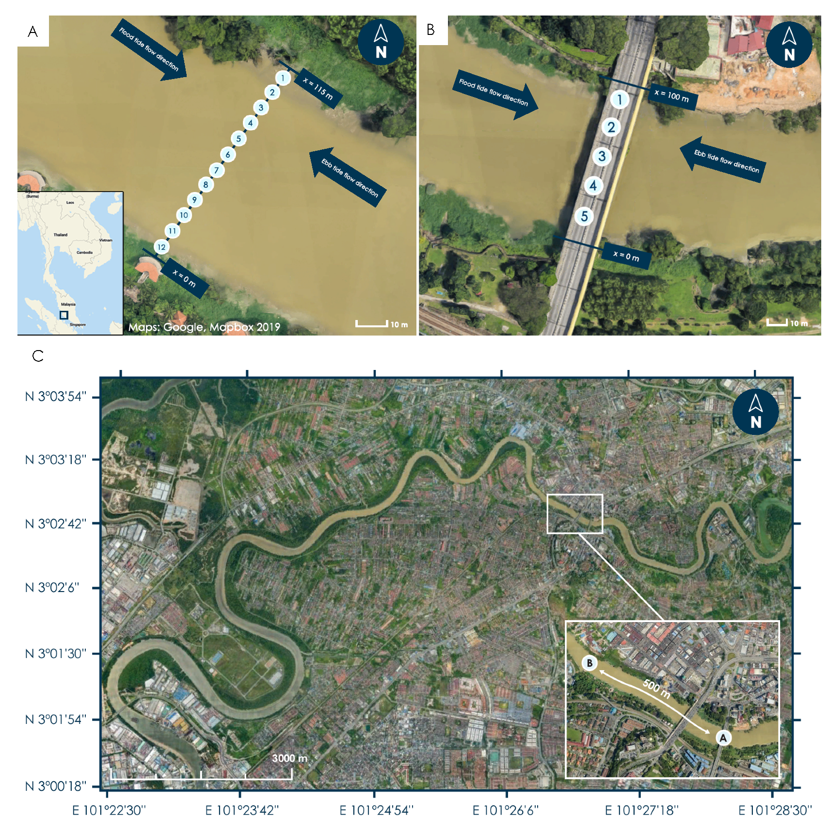
The fieldwork was conducted during the period from 29 April to 4 May 2019. The visual counting measurements were taken from the Jalan Tengku Kalana bridge (30242.5N 1012654.8E) between 09:00 and 17:00 during the entire duration of the measuring campaign. All UAV-borne measurements were taken at a location 700 m downstream (30252.9N 1012631.2E) on Klang River, on 30 April, 1 May and 4 May, between 09:00 and 17:00.
The local climate is characterised as a tropical rainforest climate according to the Köppen–Geiger classification. The cloudier part of the year starts in March and lasts until December. The city of Klang experiences an extreme seasonal variation in monthly rainfall, with the largest precipitation rates between October and December (http://www.weatherspark.com).
2.1. Aerial Survey
2.1.1. Materials
The aerial survey was performed using a DJI Phantom 4 Advanced quadcopter equipped with a 3-axis gimbal mounted 12-megapixel camera. The camera has a 1/2.3 CMOS sensor which, in combination with a lens with a 20 mm (35 mm format equivalent) focal length, provides a field of view of approximately 94°. The UAV makes use of the GPS/GLONASS positioning system in combination with a barometer and Inertial Measurement Unit (IMU), which allows for a hover accuracy of ±0.5 m vertically and ±1.5 m horizontally. The integrated Downward Vision System (DVS) offsets a hover accuracy of ±0.1 m vertically and ±0.3 m horizontally. The vision system requires a surface with a clear pattern and adequate lighting between 0.3 and 3 m distance from the UAV. Under normal conditions, the intelligent flight battery provides approximately 23 min of flight time (DJI, Shenzhen, China; http://www.dji.com).
2.1.2. Data Acquisition
To be able to make detailed cross-sectional plastic transport profiles, the aerial survey consisted of a flight path transecting the river perpendicular to its flow direction. The gimbal angle was set at 90°, at nadir, to allow for good particle shape and size detection without the need for image rectification during post-processing. To reduce inaccuracies induced by human error, the UAV’S flight path was pre-programmed using Python and flown using the Litchi waypoint mission engine (VC Technology, Inc., Brooksville, FL, USA; http://www.flylitchi.com).
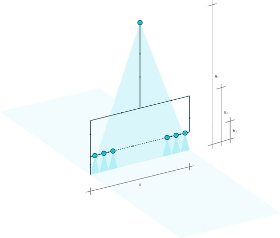
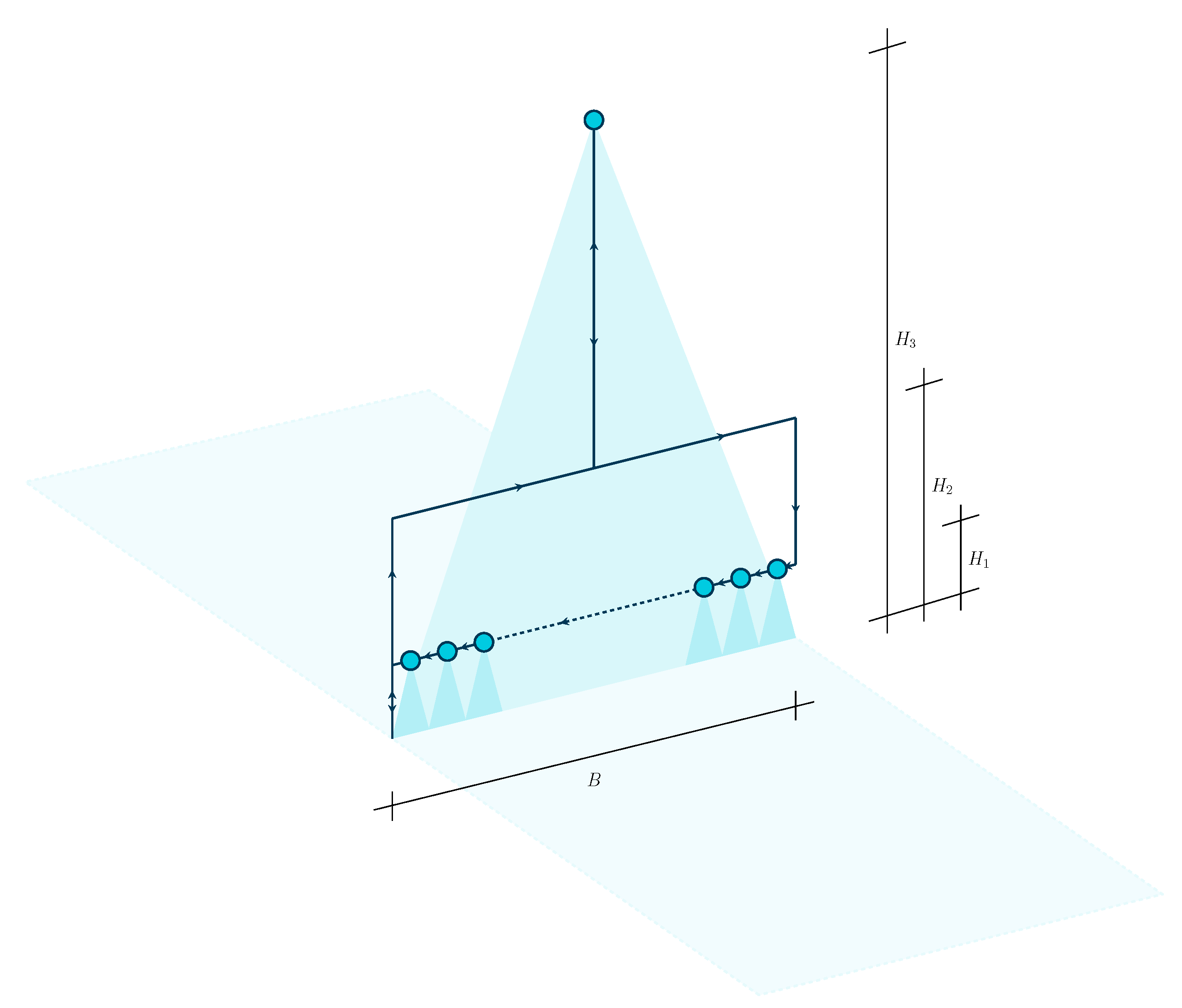
The flight path was set up at three different altitudes relative to the instantaneous water level, indicated by , and in Figure 1. Images taken at these three different altitudes serve different purposes. Stills obtained at a height of provide the basis of visual plastic counts from which plastic transport estimates can be deduced. Images obtained at altitude provide qualitative data on plastic transport “hot spots” in the river, and images obtained at provide qualitative insight into larger flow features as well as plastics stranded on the riverbanks.
During one flight, the UAV first traverses half of the river width at altitude , which is set at 15 m above water level, at a cruising speed of 13.7 km/h. Then, the UAV ascends to altitude at which it hovers for 14 s while taking still images of the total river width and the riverbanks, before descending back to and traversing the remaining half of the river cross-section at cruising speed. Upon reaching the opposite side of the river, the UAV descends further, to a height of 5 m above water level. At this height, the UAV hovers at N subsequent measuring locations along the transect for 14 s before returning to the HomePoint.
Several preliminary tests were conducted at a test site in the Netherlands to determine the ideal flight speed, camera shutter interval and altitudes and . From analysis of these preliminary tests, it was found that, to still be able to distinguish macroplastic particles (>2.5 cm) and their plastic class, the flight altitude should be in the range of 4–6 m above water level. Altitudes at which macroplastic amounts could still be determined, but could no longer be classified were in the range of 8–18 m above water level.
Based on trade-offs among flight time, pixel density, and image footprint, as well as taking into account possible machine-induced altitude inaccuracies, it was chosen to conduct the plastic transport measurements at an altitude of 5 m above water level. The qualitative “hot spot”-indicating stills were chosen to be taken at an altitude of 15 m above water level.
While flying at an altitude of 5 m, most commonly used off-the-shelf UAVs are able to take stills that have a pixel pixel density of 5–9 px/cm. These pixel densities allow for integration with available machine learning based object detection algorithms [28,29,30] and provide good conditions for plastic detection and classification by the human eye. The height was calculated based on the camera specifications of the UAV-mounted camera, the river width B and an additional width to account for the riverbank on both sides of the river. Assuming an at nadir pointing camera angle, this height can be calculated with the following equation:
with (mm) the sensor width of a 35 mm full-frame camera, (mm) the focal length of the camera in 35 mm equivalent format, B (m) the width of the river and (m) the estimated width of the riverbank. In the case study of Klang River, the river width equals approximately 115 m, which leads to an altitude of 63 m.
The amount of measuring locations (N) along the river cross-section can be calculated by dividing the river width B by the horizontal field of view (HFOV) of the used camera at a height , rounded down to the nearest integer. Based on an at nadir pointing camera angle and assuming all other gimbal axes to be equal to 0°, the horizontal field of view of the camera used can be calculated with the following equation:
The amount of measuring locations (N) along the transect can be calculated using the following equation:
For the Klang River application case, this calculation results in 12 measuring locations along the transect. Rounding down the number of measuring locations to the nearest integer implies that, in the application case of Klang River, 94% of the full river width is covered by the stills.
The hovering time of 14 s was chosen such that the altitude inaccuracy introduced by the UAV’s stabilisation procedure during hovering was as small as possible, while the amount of images obtained during the hovering time interval remained sufficiently large. In combination with a camera shutter interval of 2 s, hovering for 14 s resulted in seven or eight images at each measuring location.
Figure 2A depicts the measurement locations of the UAV-borne measurements on Klang River. The measurement locations are numbered 1–12, starting at the opposite side of the river relative to the take-off location. During measurements, the drone was facing downstream with a heading perpendicular to the main transect of the flight path. This made sure that the flow direction could be resolved from the images in the post-processing stage.
A manual record was made of the water level before take-off, after which the flight path altitudes could be adjusted accordingly. After landing, a manual record was made of the GPS altitude upon reaching the HomePoint. This altitude provides an indication of the altitude inaccuracy incurred during flight. If any significant weather changes were evident during flight, this was also manually recorded.
Besides the records that were taken manually, every image taken stores valuable metadata in Exchangeable Image File Format (EXIF), which can be accessed during post-processing of the images. The EXIF metadata stored in these image files contain all camera specifications as well as specific DJI metadata such as GPS location, flight speed, GPS altitude, all three gimbal rotations (yaw, pitch, and roll), image dimensions and the timestamp.
2.1.3. Data Processing
The collected images were subsequently divided into three categories, namely “overview measurements”, “transient measurements” and “measurements”, based on the EXIF metadata stored in each image. Images that were taken at a height higher than 1 m above the initially programmed altitude were stored as “overview measurements” and images that were recorded a flight speed larger than m/s or smaller than m/s in x-, y- or z-direction were classified as “transient measurements”. All other images were classified as “measurements”.
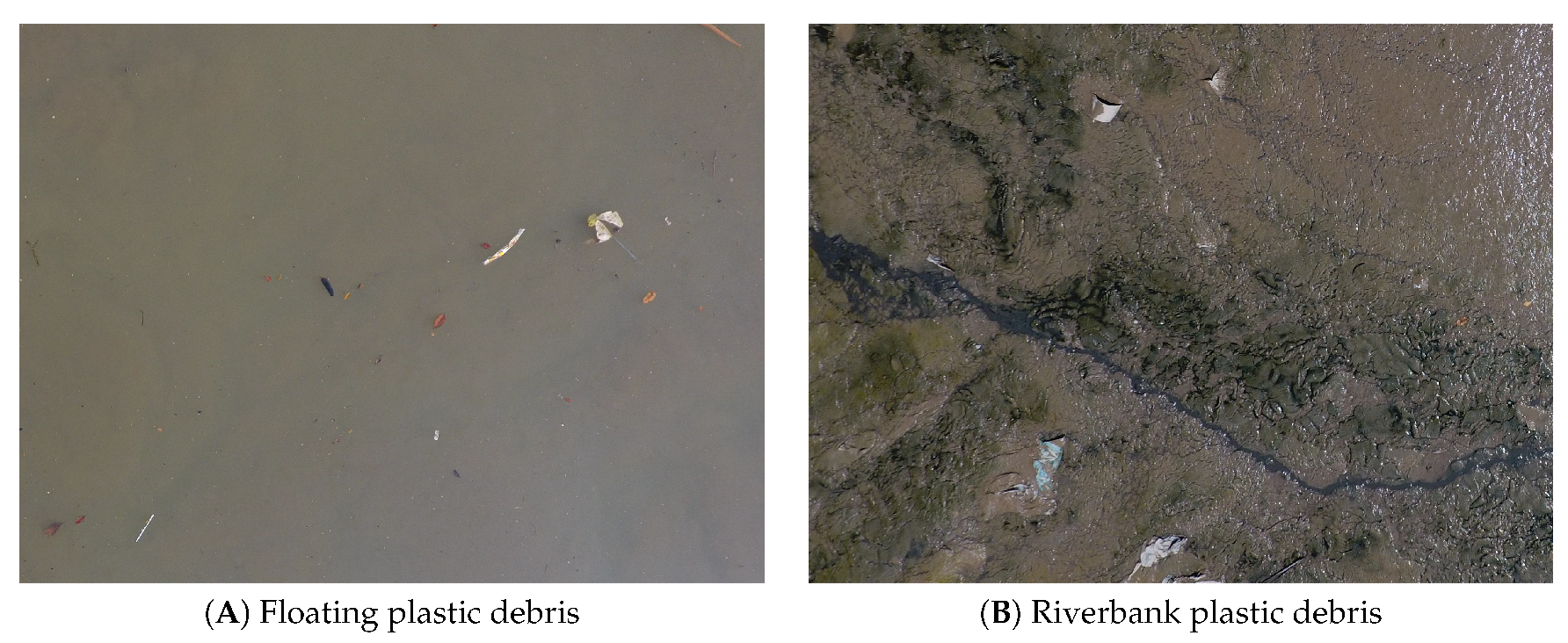
Images that were classified as “measurements” and that were part of a sampling flight for which the recorded altitude at landing (the altitude difference ) was not more than 1 m () were suitable for processing. Using the labelling tool of the online platform Zooniverse Project Builder (Citizen Science Alliance, Oxford, England; www.zooniverse.org), a small group of 15–20 volunteers tagged all visible plastics in the aerial images. The Zooniverse Project Builder platform showed these images in random order. Two different categories of plastic were distinguished: “riverbank plastics”, i.e., plastics that were stranded on or partially embedded into the riverbank, and “floating plastics”, i.e., plastics that were flowing with the current. Plastics that were flowing with the current, but were partially submerged, were also tagged as floating plastics. Debris for which the type was uncertain, was not counted.
The distinction between floating plastics and riverbank plastics was introduced because plastic debris (partially) embedded into the riverbank are distinctly different from floating plastic debris in their size, shape and colour. The distinction between floating plastic and riverbank plastic was made because we hypothesise that future machine learning object detection algorithms may be trained to recognise both classes separately. However, for the purpose of this study, only floating plastic debris was considered. Examples of aerial images with distinctly different visible plastic debris types are indicated in Figure 3.
To comply with the image size restrictions of the platform, each image was split into four smaller images prior to uploading. Even though the sizing restriction introduces the disadvantage of having to split and merge the aerial images, use of the Zooniverse platform versus other manual visual counting techniques is advantageous because exports of Zooniverse Project Builder data are directly applicable for training purposes of machine learning object detection algorithms.
2.2. Plastic Monitoring
Additional plastic measurements were done in parallel with the aerial survey procedure as a means of comparison between both methods. The measurements followed the methodology proposed by van Emmerik et al. [14], which consists of both visual counting and plastic trawling.
2.2.1. Visual Observations
Additional plastic sampling of the floating riverine plastic particles was done on five days (29 and 30 April and 2, 3 and 4 May) between 9:00 and 17:00. During each sampling day, six or seven hourly cross-sectional plastic transport profiles were made. For this, the 100-m-wide Jalan Tengku Kalana bridge was split into five segments, each measuring 20 m in width. During a time frame of 2 min, a team of two observers counted and classified all plastics passing through a segment. Each floating or partially submerged particle that could be identified as plastic was counted, independent of its size. If the debris type was uncertain, it was not counted as plastic.
Velocity estimates were done with a visual approach for each segment after each visual count. Observers traced a plastic particle along a 10-m transect perpendicular to the bridge and noted the time necessary to traverse this transect. Estimates obtained using this method were timed 4–7 min apart.
The segments were observed sequentially, starting at the southern side of the bridge. Counting was done facing upstream since a walkway on the upstream side of the bridge provided shelter from rain and sun. This allowed us to make continuous visual counts regardless of the weather. The exact observation locations on the bridge are indicated in Figure 2B.
Based on visual inspection, it was estimated that the turbidity of the water was relatively stable during the measuring period. With this turbidity, it was estimated that any plastics in the upper 20 cm of the water column were clearly visible. The average height of the bridge above the instantaneous water level was estimated at 12 m, with observed water level fluctuations of approximately 2 m. The minimum size of debris that could still be distinguished at this height was estimated at 2 cm.
2.2.2. Plastic Sampling
Plastic sampling was done using a static bridge-mounted two-layer trawl. The two-layer trawl consisted of a framework to which two 2-m-long nets were attached. The framework was made up of two vertically connected rectangular aluminium frames, the top frame measuring 0.67 m by 0.67 m, and the bottom frame measuring 0.67 m by 0.5 m. Two 0.67-m-long aluminium tubes with floaters were attached perpendicularly to the top frame with t-joints, at a distance of 0.17 m from the top of the upper frame. With this set-up, the top frame sampled the upper 0.5 m of the water column and the bottom frame sampled the water column between 0.5 m and 1.0 m depth. The chosen net mesh size of 2.5 cm was an optimisation between the desired size fraction of plastic catch and manageability of the trawl due to the drag force acting on the nets.
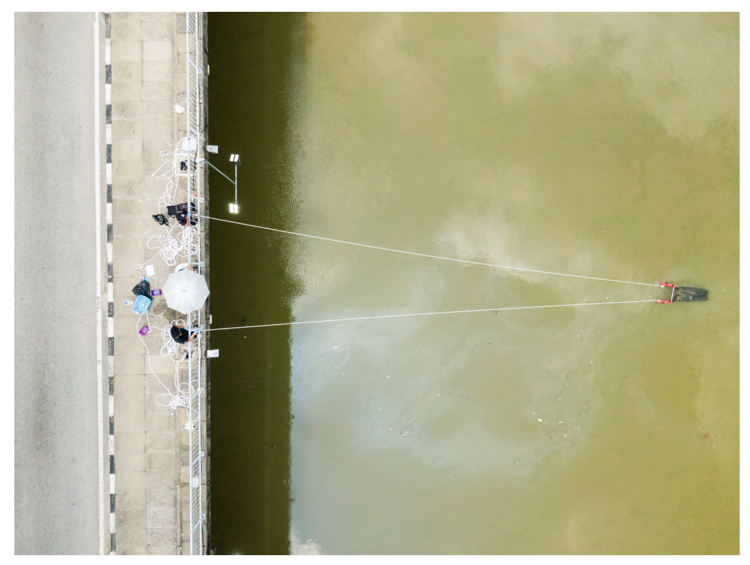
The trawling location was based on the prevailing flow direction and the observed location of the preferential path of the plastic debris, taking into account navigation routes (Figure 4). Depending on the flow velocity and the plastic load, trawl deployment lasted between 10 and 20 min. Debris samples were analysed following a three-step procedure. Firstly, the retrieved sample was divided into two categories: organic debris and plastic debris. Secondly, the debris in both categories was subsequently weighed using a digital scale. As a last step, plastic concentrations were calculated based on the trawled plastic samples. The plastic concentration was calculated from the trawled plastic mass as follows:
with plastic concentration (#/m3), area of the trawl (m2), the number of plastic particles , flow velocity v (m/s) and the trawl deployment time t (s).
3. Results
3.1. Plastic Transport Profiles
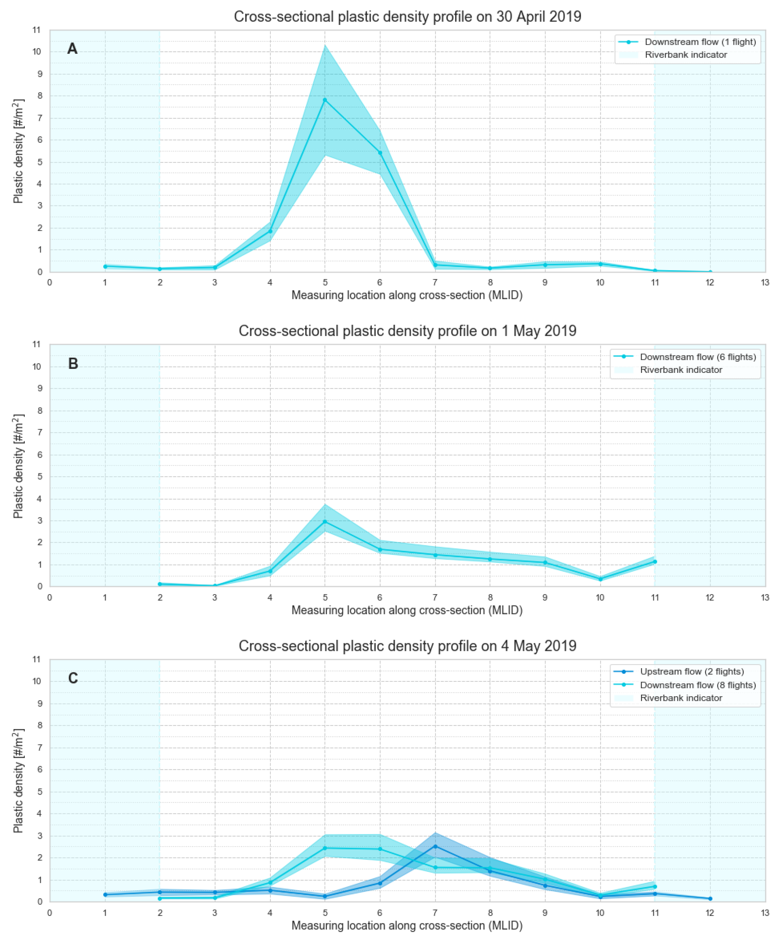
Since the Klang River is a tide-dominated river, two apparent flow directions were observed: (1) an upstream flow (flood current) and (2) a downstream flow (ebb current). Although a tidal cycle was observed on all days, plastic quantities were only determined for observations during high tide on 30 April and 1 May. On 4 May, plastic quantities were measured during flow in both directions.
The highest plastic densities are observed in the middle part of the river on all monitored days. On 30 April and 1 May, the highest plastic densities were found approximately 48 m from the southern riverbank (ML5). This is to be expected, because it is known from previous research that the variation in plastic transport in rivers is mainly influenced by the surface flow velocity [13,14]. During the entire measuring period the flow velocity was highest in the middle part of the river, as was measured with the visual survey. The tidal cycle likely influences the preferential path of the plastics in the river, as is suggested by Figure 5, since during low tide the highest plastic densities were found approximately 67 m from the southern riverbank (ML7).
Figure 5 depicts the absolute cross-sectional mean plastic density profiles on 30 April, 1 May and 4 May 2019 as measured with the aerial survey. The mean plastic densities at the measured height are indicated. The maximum of the error band in Figure 5 indicates the maximum of the plastic density at height or the plastic density at height plus measurement error, and the minimum of the error band indicates the minimum of the plastic density at height and the plastic density at height minus the measurement error. For the calculation of these profiles, only floating plastic debris was taken into account.
3.2. Altitude Inaccuracies
The influence of the recorded altitude difference after landing on the plastic density was estimated by calculating the plastic density for the case that the actual height at which the UAV was flying during the aerial survey was . All other factors considered constant, this altitude difference leads to a plastic density error induced by a difference in image footprint. To estimate this error, the plastic density at height was calculated for each picture and compared with the plastic density calculated based on the recorded height .
On average, the largest absolute altitude differences were recorded on 4 May, with a daily mean altitude difference of 0.47 m. For comparison, on 1 May, the mean altitude difference was 0.32 m. During the one flight executed on 30 April for which the plastics were classified, the altitude difference was zero. The mean absolute error in the plastic density due to the altitude difference on 1 May was 14.4%, whereas the maximum error recorded on 1 May amounted to 19.0%. In comparison, on 4 May, the mean absolute error in plastic density due to the introduction of an altitude difference amounted to 19.5%, and the maximum error was equal to 44.0%.
3.3. Cumulative and Normalised Plastic Transport Distributions
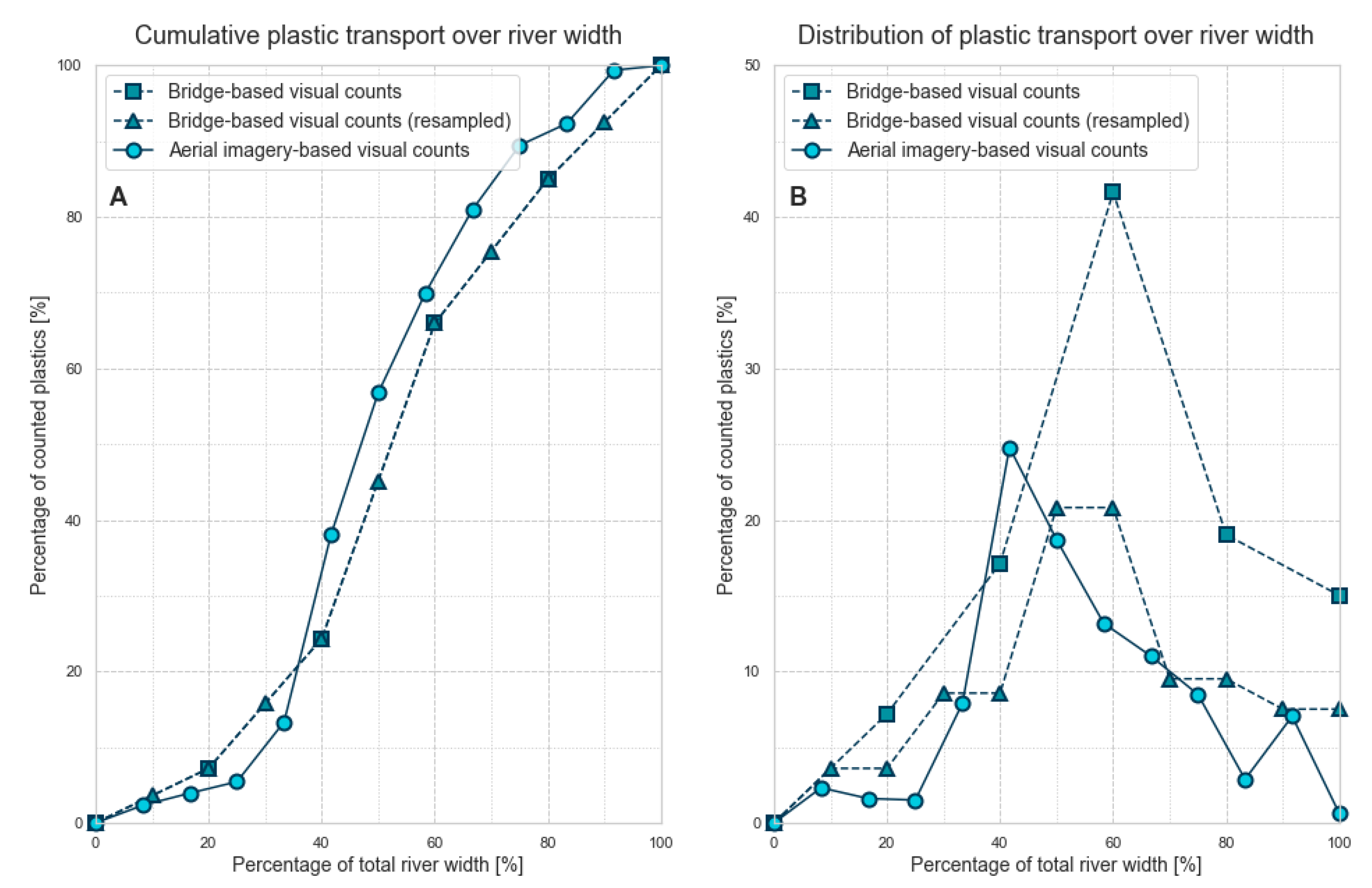
The normalised cumulative plastic transport and the normalised distribution of plastic transport over the river width, measured with both the aerial survey and the bridge-based visual survey, show similar trends (R = 0.97, RMSE = 6.7%). Although this trend is evident visually from the curves presented in Figure 6, it is also clearly visible that the difference in spatial resolution over the river width introduces an asymmetry between the distribution of plastic transport over the river width. The plastic densities obtained with the visual survey, as shown in Figure 6, were resampled for a more accurate comparison between both methods. The resampled data provide plastic counts in 10 segments, each containing half of the plastic counts in comparison with the original data.
3.4. Spatiotemporal Distribution
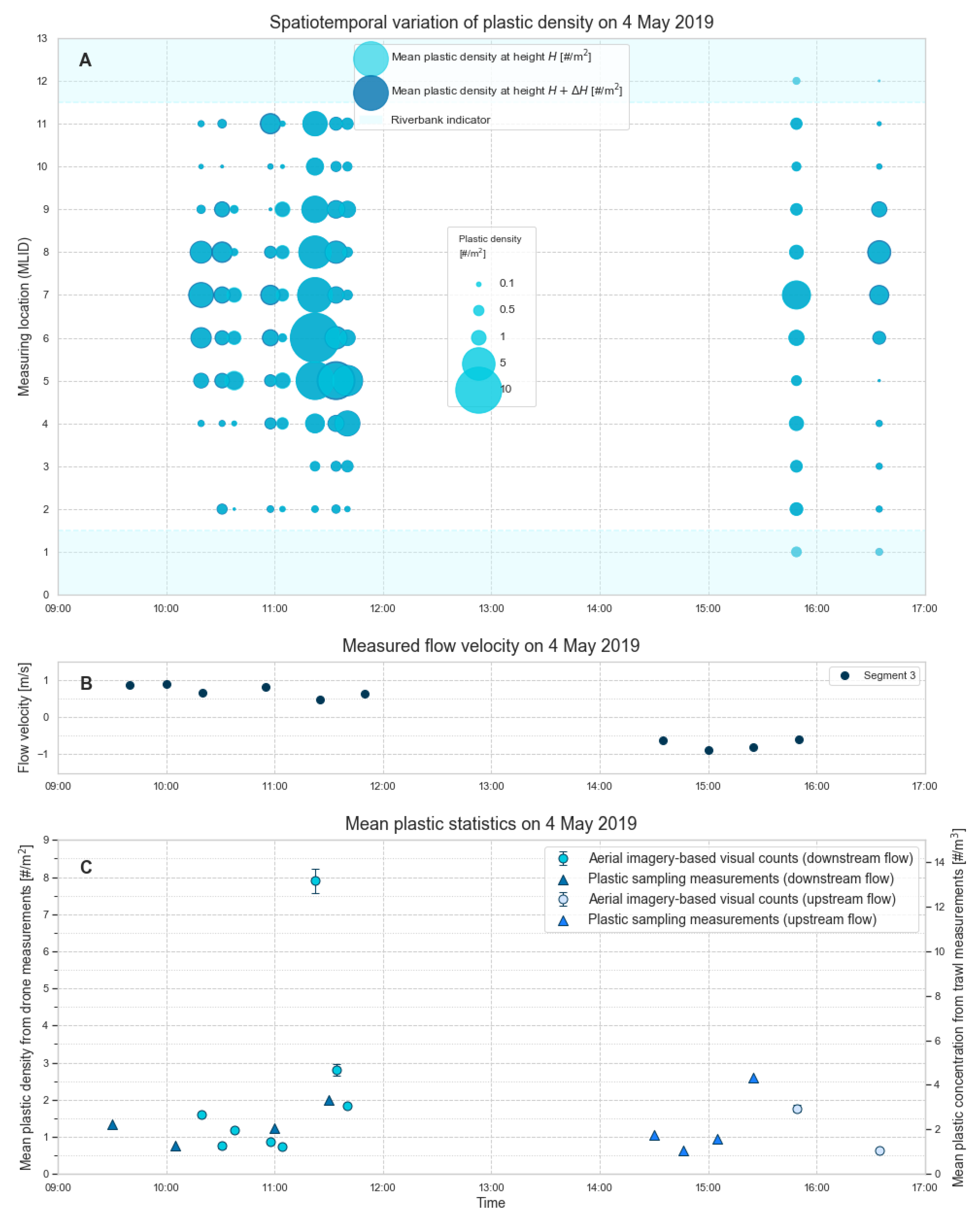
Measured plastic concentrations vary both in time and space during the entire measuring period. The spatiotemporal distribution of the plastic concentrations obtained from the UAV-based approach on 4 May 2019 is depicted in Figure 7A. Plastic amounts increase suddenly between 11:00 and 12:00, although manual velocity measurements do not indicate a velocity increase. Between 11:45 and 15:00, altitude inaccuracies were outside of the 1.0 m range, thus no measurements are presented within this time frame.
The mean plastic concentrations obtained by trawling were set out against the plastic densities obtained with the aerial survey in time (Figure 7C). For the determination of the plastic concentration from trawl measurements, only the plastic counts in the upper frame of the trawl were used (upper 0.5). These are comparable to the plastic counts from the aerial survey, since we estimated that on average the upper 0.2 m of the water column was visible from the aerial images during the entire measuring period. Since trawling was always done at the location with the highest plastic transport rates, the trawling data most accurately represent the plastic transport in Segment 3. The flow velocity was therefore interpolated based on flow velocity measurements from Segment 3 in order to calculate the plastic concentrations. The plastic densities per flight were calculated from solely the plastic counts in the middle section of the river for better comparison. Examining these plastic statistics, we see that, although the units in which the plastic statistics are expressed are not equal, they follow the same overall trend. For the presented application case on Klang River, no hydrological records were available during the monitoring period. If consistent water level records or discharge records are available, the main plastic statistics can be expressed in the same units, which allows for a more detailed comparison between the two methods.
4. Discussion
4.1. Altitude Inaccuracies
In this paper, we have based the measure of the altitude inaccuracy induced during flight on the manually recorded altitude after landing. It must be noted that the altitude difference recorded after landing only gives an indication of the order of magnitude of the introduced altitude difference, as the instantaneous altitude difference at a measuring location could still be higher or lower. Furthermore, we only analysed aerial images taken during flights after which the recorded absolute altitude difference was no larger than 1.0 m. During the entire duration of the fieldwork, however, altitude differences of up to 3.0 m were recorded. This is not taken into account for the presented error estimates.
We expect that these altitude differences are mainly induced by the UAV’s internal stabilisation procedure. When flying with the DJI Phantom 4 Advanced, three flight modes are available: P-mode (positioning), A-mode (altitude) and F-mode (function). Normally, P-mode is activated, as was the case during the application on Klang River. In P-mode, three different states are discerned, one of which is automatically selected depending on GPS signal strength and Downward Vision Positioning sensors. When GPS and Vision Positioning are both available, the aircraft is using GPS positioning (P-GPS mode). If the GPS signal strength is not sufficient but the Vision Positioning System is available, then the Vision Positioning System is used (P-OPTI mode). When the GPS signal is weak and lighting conditions are too dark or too light for the Vision Positioning System, the aircraft will use only the internal barometer for altitude stabilisation (P-ATTI mode). In the Klang River application case, weather conditions were rapidly changing between and during flights. Furthermore, the Vision Positioning System was unavailable during all flights, since the flight altitude was larger than 3 m. When a thick cloud cover was present, the GPS signal was too weak and P-ATTI mode was enabled. If this was accompanied by a sudden temperature drop or increase, the internal barometer recorded an altitude change which triggered the stabilisation procedure, even though an actual altitude change had not occurred. In these types of climates, it is difficult to mitigate this stabilisation effect when using off-the-shelf drones. However, it is possible to record the flight altitude more accurately by introducing an external altitude meter as a payload. A good option would be using real-time kinematic GPS, which has an altitude accuracy of within a meter. Another option would be a set-up with a laser total station theodolite at the river bank and a prism mounted on the UAV, with which millimetre to centimetre accuracy can be achieved.
Improving altitude accuracy is strongly recommended for future research, although improvements could require the use of custom drones instead of off-the-shelf models. The use of custom drones could in turn have implications on the accessibility of the methodology to the broader public, which is possibly undesirable. Alternatively, one could make use of higher resolution cameras in combination with higher flight altitudes. If similar pixel densities can be obtained when flying at larger altitudes using higher resolution cameras, altitude differences in the order of 1–3 m have a relatively smaller influence on error estimates. Additionally, the larger spatial coverage could be beneficial for plastic debris monitoring of some of the top polluting rivers, as estimated by Lebreton et al. [6], many of which are several kilometres in width.
4.2. Comparison of UAV-Based Approach with Visual Counting Survey
Both the cumulative and normalised plastic transport distributions presented in Figure 6 show obvious differences between estimates obtained by using the UAV-based approach and estimates obtained by visual counting.
The plastic distribution might show differences between both surveys because the amount of time that an upstream current was observed during the monitoring period was higher for the visual survey than for the aerial survey. The percentage of observations during an upstream current was 29.3% for the visual survey, while this was 19.5% for the aerial survey. As deduced from Figure 5C, the preferential path of the plastics shifts from the southern riverbank to the northern riverbank during a tidal cycle, which leads to a more uniform distribution for the visual survey when averaging over the entire duration of the monitoring campaign.
Moreover, the observed differences in the distribution of plastic transport obtained with the visual survey could be explained by the distance between both monitoring sites. The distance between the Jalan Tengku Kalana bridge site and the aerial survey site was approximately 500 m. At such distances, the asymmetry in the plastic distribution could be (partly) dismissed as natural variability. Besides the differences in spatial resolution of both methods, asymmetries in the plastic transport distribution can be introduced due to the difference in nature of the sampling methods.
Lastly, as observers were visually counting the plastic debris amounts, they were simultaneously classifying the plastics. This can introduce an error because, in fast-flowing currents, it is likely that not all plastics are able to be counted and classified within the time frame that the plastic debris is visible. This leads to a bias towards the segments with a lower flow velocity. On the other hand, the raw aerial images obtained during the visual survey can be counted and interpreted again, either manually or automatically. The option to revisit raw data and correct for any errors will decrease the uncertainty. The visual survey-approach can therefore not just unequivocally be used as a baseline for quantitative comparison, as the visual survey also has its limitations. Comparison of the trend of mean plastic statistics, both in time and in space, is therefore sufficient for the purpose of this study. Integration with machine learning object detection algorithms and machine learning-based Particle Imaging Velocimetry (PIV) techniques will be necessary to obtain comparative plastic fluxes and ensure scale-up of the methodology.
4.3. Observer Bias
An interesting parameter to asses the observer bias is the difference in plastic counts between subsequent images in the same population. To show the largest differences between these counts, we look at the flight with the highest total amount of plastic counts, which is the flight conducted on 4 May at 11:22. The largest measured difference in plastic counts between subsequent images during this flight was 39 particles. Subsequent images were taken 2 s apart. Although these relatively large differences in successive images can be accurate in case of higher flow velocities, it most likely indicates an observer bias in plastic counts. This presumption is confirmed by looking at the records of the measured flow velocity (Figure 7), which shows that the flow velocity is smaller during previous flights, while these do not show large differences in plastic counts between subsequent images.
Another interesting parameter to potentially assess the observer bias is the increase or decrease of debris amounts between subsequent flights. Figure 7A shows the spatiotemporal variation of the plastic density as measured using the aerial survey, not taking into account the direction of the plastic transport. In Figure 7A, we see that, at 11:22, a large increase in plastic density was observed from the aerial survey. This seems out of the ordinary when looking at the preceding and following flights. This sudden increase and decrease of plastic counts can indicate an event with a sudden increase of the plastic debris amounts, but can also be (partly) induced during data processing. The aerial images were randomised during the labelling process, thus it is not likely that the sudden increase is an artefact of some labelling bias. Furthermore, the overall increase in plastic density is uniform over the river width. This indicates that these sudden changes in plastic amounts most likely represent an actual event.
Observer bias is possibly exacerbated by three factors. During sunny, cloudless weather conditions, sun glint is visible in the images. This not only leads to local loss of information, but in some cases also casts a shadow on small organic particles present on the water surface. In such cases, these particles resemble small dark plastic particles on the water surface, which leads to classification errors. Secondly, the images are not processed in the same order as they were obtained, which makes it more difficult for a human observer to discern actual plastic particles from sun glint. Lastly, any observer bias already present is exaggerated by splitting and combining the original images for the Zooniverse platform.
There are several ways to reduce the bias introduced by sun glint on the surface. The easiest way to reduce sun glint is to make use of polarising filters when flying in sunny conditions. This directly reduces the appearance of sun glint [31]. A disadvantage of using polarising filters, however, are that they cannot be “turned off” during flight. In climates where weather conditions can rapidly change this poses a risk, because information loss can occur if the polarising filter is too strong. Furthermore, polarising filters only work as desired at a specific orientation and might even work adversely at some orientations. Another way to reduce sun glint is to change the pitch angle of the UAV-mounted camera [32]. When the pitch angle is pointing at nadir, the effect of sun glint is strongest. If the pitch angle is changed to, e.g., 10° from nadir, this could already lead to a reduction of the sun glint effect. The main disadvantage of this method is that plastic particles might appear distorted, making it more difficult for observers and machine learning object detection algorithms to classify the plastic debris. To be able to assess whether this effect is significant at a flight altitude of 5 m, further research is recommended.
4.4. Outlook
Upon first application of the presented methodology on Klang River, Malaysia, we found that the trend in cross-sectional plastic density obtained with the proposed aerial survey methodology strongly resembles the trend in plastic flux estimates obtained with a visual survey. For reliable, direct comparisons, it is recommended to couple the obtained plastic densities to consistent hydrological data, which highlights the importance of the availability of such data. In the future, the aerial images obtained with the presented protocol could provide the basis for, e.g., velocity data, by using them as a basis for PIV measurements. Several papers have previously been published implementing such PIV techniques based on aerial images in outdoor environments [33,34,35,36]. This could significantly increase the accuracy and spatial resolution of velocity measurements.
Although the presented methodology is simple, it provides both quantitative data on plastic transport and qualitative data on the amount of plastics present on the riverbanks, and accommodates integration with machine learning approaches for object detection. Additionally, it is easy to obtain extra (meta)data by adding more measuring equipment as a payload, such as a single-beam sonar [37]. Altitude accuracy can potentially be improved by using e.g., real-time kinematic GPS or a laser total station in combination with a UAV-mounted prism. Moreover, error estimates could possibly be reduced by using a UAV with a higher quality camera flying at a higher altitude, for which altitude differences in the range of 1–5 m lead to smaller error estimates.
The presented methodology has been tested for river widths up to 200 m, and in theory it can be applied to river widths up to 500 m if the same hovering time, flight speed and altitudes are used. When looking at the top 20 polluting rivers, as predicted by Lebreton et al. [6], it is evident that this is very small compared to widths of several kilometres that some of these top polluters have. It is important to further research the possibility to apply the proposed aerial survey techniques in these very wide rivers, since practical considerations may restrict application in such cases. Use of higher resolution cameras in combination with larger flight altitudes could partly provide a solution to these practical considerations.
Continuous monitoring would allow more accurate measurements of the evolution of plastic transport over time. In sufficiently narrow rivers, this could be achieved by using tethered drones with power systems positioned on the riverbanks. Unmanned tethered blimps have been used for similar monitoring tasks in the marine environment, which could provide lessons learned [38]. In wider rivers however, this would require usage of a floating object to carry the power systems, which might deform the flow and plastic transport locally. In such cases, it is advised to use tailor-made drones that are built for the specific application, although the methodology presented in this paper might still be applied on a basic level.
Other future perspectives related to the presented work should involve integration with machine learning algorithms for automatic object detection and classification. This can be applied for the detection of floating plastics as well as riverbank plastics [20]. The presented work merely presents a methodology for measuring the spatiotemporal variation of plastic particles, whereas the full potential of the methodology can be realised when combined with machine learning object detection methods and PIV techniques. Volunteers indicated that floating debris was generally easy to classify because of a sharp contrast in colour between debris and water column and the clearly distinguishable shapes of common plastic debris types. Riverbank plastics, however, had more capricious shapes and the transition between debris and riverbank was often unclear. When training object detection algorithms, this should be taken into account.
5. Conclusions
This paper presents a first methodology to quantify floating riverine plastic transport at monitoring sites without any existing infrastructure by use of an off-the-shelf UAV. Use of this methodology opens up many new possibilities to further substantiate the origin, distribution and fate of riverine plastic debris with fieldwork measurements.
The use of an automated flight path as a monitoring technique provides an easy, adaptable and relatively cheap method to monitor floating riverine plastic debris at locations without existing infrastructure. The aerial images obtained with the UAV-based protocol have pixel densities that allow for integration with existing machine learning object detection algorithms, which could drastically reduce the observer bias in future applications and thus lead to more accurate estimations of worldwide riverine plastic debris transport.
The main disadvantage of the proposed methodology is that the application and accuracy of the method are strongly dependent on weather conditions. UAVs should not be used in severe weather conditions, including wind speeds exceeding 10 m/s, as well as during rain, snow, thunderstorms, and fog. In climates that are highly susceptible to sudden weather changes, the altitude accuracy decreases significantly. Coincidentally, many of the top polluting rivers, as estimated by Lebreton et al. [6], are located in countries with highly variable climatic conditions. Although the internal stabilisation procedure inducing the altitude inaccuracy cannot be changed in off-the-shelf UAVs, its effects on the obtained data can be mitigated if the altitude can be monitored more accurately from the drone, e.g. by use of real-time kinematic GPS. Use of higher resolution cameras in combination with larger flight altitudes could also potentially reduce the effects of these altitude inaccuracies. Furthermore, the presented methodology can easily be extended to also monitor many other parameters by the addition of a suitable payload.
Overall, it can be concluded that the use of UAVs shows great potential for monitoring of the spatiotemporal distribution of riverine plastic debris. In the Klang River application case, the pattern of the plastic density profile measured with the aerial survey strongly resembles the pattern of the plastic transport profile measured with the visual counts and the plastic concentrations obtained through plastic sampling. Direct comparisons, however, are difficult to make on account of the lack of hydrological data during the measurement period. In future application cases, it is essential that the obtained plastic statistics can be coupled to this hydrological data in order to make more detailed comparisons on the accuracy of both protocols. Partly, such data can be obtained directly from the aerial images by using PIV techniques.
In this paper, we demonstrate that UAVs offer promising new possibilities for riverine plastic transport monitoring. UAVs can overcome practical challenges associated with current monitoring methods, which is especially of interest to wide, remote or inaccessible rivers. The method presented here is simple, adaptable and can be used in remote areas without many difficulties. It is therefore advantageous in efforts to scale up river plastic monitoring efforts around the world, and will enable making more accurate estimations of riverine plastic transport on a higher spatial and temporal scale.
Author Contributions
Conceptualisation, M.G., R.d.V., and T.v.E.; methodology, M.G. and R.d.V.; data collection, M.G., T.v.E., and M.S.b.A.R.; software, M.G.; formal analysis, M.G.; writing—original draft preparation, M.G.; writing—review and editing, R.d.V., T.v.E., and M.S.b.A.R.; and visualisation, M.G.; supervision, T.v.E.
Funding
This research received no external funding.
Acknowledgments
We would like to thank the donors of The Ocean Cleanup who helped fund this study. The execution of the fieldwork would not be possible without our partners at Beyond Horizon Technologies Sdn Bhd and the Universiti Putra Malaysia (UPM). We are very grateful to M. Fadzly B. M. Khalil for making the drones and pilots available. We thank Nerson Bidin and M. Roslan Anan, the diligent drone pilots from Beyond Horizon Technologies Sdn Bhd, for the execution of the aerial survey. From UPM, we thank Mohd. Shahrizal Ab Razak, Ezanee Bin Gires, Hafíz Rashidi B. Harun, Syaril Azrad Md. Ali, and the student team of UPM for their hard work during the data collection for the visual survey. We gratefully acknowledge the Zooniverse Project Builder platform, which was used for classification of the plastic debris, and all volunteers who helped classify the plastics in the thousands of images. Finally, we thank Arsalan Ahmed Othman and the three anonymous reviewers for their valuable comments.
Conflicts of Interest
The authors declare no conflict of interest.
Abbreviations
The following abbreviations are used in this manuscript:
| EXIF | Exchangeable Image File Format |
| GPS | Global Positioning System |
| GLONASS | Global Navigation Satellite System |
| HFOV | Horizontal Field Of View |
| IMU | Inertial Measurement Unit |
| PIV | Particle Image Velocimetry |
| UAV | Unmanned Aerial Vehicle |
References
- PlasticsEurope. Plastics—The Facts 2018, an Analysis of European Plastics Production, Demand and Waste Data; Technical report; PlasticsEurope, Association of Plastic Manufacturers: Brussels, Belgium, 2018. [Google Scholar]
- Ó Conchubhair, D.; Fitzhenry, D.; Lusher, A.; King, A.L.; van Emmerik, T.; Lebreton, L.; Ricaurte-Villota, C.; Espinosa, L.; O’Rourke, E. Joint effort among research infrastructures to quantify the impact of plastic debris in the ocean. Environ. Res. Lett. 2019, 14, 065001. [Google Scholar] [CrossRef] [Green Version]
- Geyer, R.; Jambeck, J.R.; Law, K.L. Production, use, and fate of all plastics ever made. Sci. Adv. 2017, 3, e1700782. [Google Scholar] [CrossRef] [PubMed]
- Galloway, T.S.; Cole, M.; Lewis, C. Interactions of microplastics debris throughout the marine ecosystem. Nat. Ecol. Evol. 2017, 1, 0116. [Google Scholar] [CrossRef] [PubMed]
- Wang, J.; Tan, Z.; Peng, J.; Qiu, Q.; Li, M. The behaviors of microplastics in the marine environment. Mar. Environ. Res. 2016, 113, 7–17. [Google Scholar] [CrossRef] [PubMed]
- Lebreton, L.C.; van der Zwet, J.; Damsteeg, J.W.; Slat, B.; Andrady, A.; Reisser, J. River plastic emissions to the world’s oceans. Nat. Commun. 2017, 8, 15611. [Google Scholar] [CrossRef] [PubMed]
- Schmidt, C.; Krauth, T.; Wagner, S. Export of Plastic Debris by Rivers into the Sea. Environ. Sci. Technol. 2017, 51, 12246–12253. [Google Scholar] [CrossRef] [PubMed]
- Jambeck, J.R.; Geyer, R.; Wilcox, C.; Siegler, T.R.; Perryman, M.; Andrady, A.; Narayan, R.; Law, K.L. Plastic waste inputs from land into the ocean. Science 2015, 347, 768–771. [Google Scholar] [CrossRef]
- GESAMP. Sources, Fate and Effects of Microplastics in the Marine Environment: Part Two of a Global Assessment; IMO/FAO/UNESCO-IOC/UNIDO/WMO/IAEA/UN/ UNEP/UNDP Joint Group of Experts on the Scientific Aspects of Marine Environmental Protection; Rep. Stud. GESAMP No. 93; International Maritime Organization: London, UK, 2016; 220p. [Google Scholar]
- Blettler, M.C.; Abrial, E.; Khan, F.R.; Sivri, N.; Espinola, L.A. Freshwater plastic pollution: Recognizing research biases and identifying knowledge gaps. Water Res. 2018, 143, 416–424. [Google Scholar] [CrossRef] [Green Version]
- Cheshire, A.; Adler, E.; Barbière, J.; Cohen, Y.; Evans, S.; Jarayabhand, S.; Jeftic, L.; Jung, R.T.; Kinsey, S.; Kusui, T.; et al. UNEP/IOC Guidelines on Survey and Monitoring of Marine Litter; IOC Technical Series No. 83: xii + 120; United Nations Environment Programme/Intergovernmental Oceanographic Commission: Paris, France, 2009. [Google Scholar]
- Rech, S.; Macaya-Caquilpán, V.; Pantoja, J.; Rivadeneira, M.; Madariaga, D.J.; Thiel, M. Rivers as a source of marine litter—A study from the SE Pacific. Mar. Pollut. Bull. 2014, 82, 66–75. [Google Scholar] [CrossRef]
- González-Fernández, D.; Hanke, G.; Tweehuysen, G.; Bellert, B.; Holzhauer, M.; Palatinus, A.; Hohenblum, P.; Oosterbaan, L. Riverine Litter Monitoring—Options and Recommendations. MSFD GES TG Marine Litter Thematic Report; Technical Report, EUR 28307; EUR: Luxembourg, Belgium, 2017. [Google Scholar]
- van Emmerik, T.; Kieu-Le, T.C.; Loozen, M.; van Oeveren, K.; Strady, E.; Bui, X.T.; Egger, M.; Gasperi, J.; Lebreton, L.; Nguyen, P.D.; et al. A Methodology to Characterize Riverine Macroplastic Emission Into the Ocean. Front. Mar. Sci. 2018, 5, 372. [Google Scholar] [CrossRef]
- van Emmerik, T.; Loozen, M.; van Oeveren, K.; Buschman, F.; Prinsen, G. Riverine plastic emission from Jakarta into the ocean. Environ. Res. Lett. 2019, 14, 084033. [Google Scholar] [CrossRef] [Green Version]
- Jones, G.P., IV; Pearlstine, L.G.; Percival, H.F. An Assessment of Small Unmanned Aerial Vehicles for Wildlife Research. Wildl. Soc. Bull. 2006, 34, 750–758. [Google Scholar] [CrossRef]
- Gonzalez, L.F.; Montes, G.A.; Puig, E.; Johnson, S.; Mengersen, K.; Gaston, K.J. Unmanned Aerial Vehicles (UAVs) and Artificial Intelligence Revolutionizing Wildlife Monitoring and Conservation. Sensors 2016, 16, 97. [Google Scholar] [CrossRef] [PubMed]
- Chen, B.; Yang, Y.; Wen, H.; Ruan, H.; Zhou, Z.; Luo, K.; Zhong, F. High-resolution monitoring of beach topography and its change using unmanned aerial vehicle imagery. Ocean. Coast. Manag. 2018, 160, 103–116. [Google Scholar] [CrossRef]
- Turner, I.L.; Harley, M.D.; Drummond, C.D. UAVs for coastal surveying. Coast. Eng. 2016, 114, 19–24. [Google Scholar] [CrossRef]
- Martin, C.; Parkes, S.; Zhang, Q.; Zhang, X.; McCabe, M.F.; Duarte, C.M. Use of unmanned aerial vehicles for efficient beach litter monitoring. Mar. Pollut. Bull. 2018, 131, 662–673. [Google Scholar] [CrossRef] [PubMed] [Green Version]
- Chabot, D.; Dillon, C.; Ahmed, O.; Shemrock, A. Object-based analysis of UAS imagery to map emergent and submerged invasive aquatic vegetation: A case study. J. Unmanned Veh. Syst. 2017, 5, 27–33. [Google Scholar] [CrossRef]
- Bloom, D.; Butcher, P.A.; Colefax, A.P.; Provost, E.J.; Cullis, B.R.; Kelaher, B.P. Drones detect illegal and derelict crab traps in a shallow water estuary. Fish. Manag. Ecol. 2019, 26, 311–318. [Google Scholar] [CrossRef]
- Ezat, M.A.; Fritsch, C.J.; Downs, C.T. Use of an unmanned aerial vehicle (drone) to survey Nile crocodile populations: A case study at Lake Nyamithi, Ndumo game reserve, South Africa. Biol. Conserv. 2018, 223, 76–81. [Google Scholar] [CrossRef]
- Andrew, M.E.; Shephard, J.M. Semi-automated detection of eagle nests: an application of very high-resolution image data and advanced image analyses to wildlife surveys. Remote Sens. Ecol. Conserv. 2017, 3, 66–80. [Google Scholar] [CrossRef] [Green Version]
- Kellenberger, B.; Marcos, D.; Lobry, S.; Tuia, D. Half a Percent of Labels is Enough: Efficient Animal Detection in UAV Imagery using Deep CNNs and Active Learning. arXiv 2019, arXiv:1907.07319. [Google Scholar] [CrossRef]
- Lyons, M.B.; Brandis, K.J.; Murray, N.J.; Wilshire, J.H.; McCann, J.A.; Kingsford, R.T.; Callaghan, C.T. Monitoring large and complex wildlife aggregations with drones. Methods Ecol. Evol. 2019, 10, 1024–1035. [Google Scholar] [CrossRef] [Green Version]
- European Commission Joint Research Center. MSFD Technical Subgroup on Marine Litter (TSG-ML). Guidance on Monitoring of Marine Litter in European Seas. Technical Report, EUR 26113 EN- Joint Research Center. 2013. Available online: https://ec.europa.eu/jrc/sites/jrcsh/files/lb-na-26113-en-n.pdf (accessed on 20 June 2019).
- Ren, S.; He, K.; Girshick, R.B.; Sun, J. Faster R-CNN: Towards Real-Time Object Detection with Region Proposal Networks. IEEE Trans. Pattern Anal. Mach. Intell. 2015, 39, 1137–1149. [Google Scholar] [CrossRef] [PubMed]
- Khashman, A. Automatic detection, extraction and recognition of moving objects. Int. J. Syst. Appl. Eng. Dev. 2008, 2, 43–51. [Google Scholar]
- Etten, A.V. You Only Look Twice: Rapid Multi-Scale Object Detection In Satellite Imagery. arXiv 2018, arXiv:1805.09512. [Google Scholar]
- Tyler, S.; Jensen, O.P.; Hogan, Z.; Chandra, S.; Galland, L.M.; Simmons, J.; Team, T.T.R. Perspectives on the Application of Unmanned Aircraft for Freshwater Fisheries Census. Fisheries 2018, 43, 510–516. [Google Scholar] [CrossRef]
- Joyce, K.E.; Duce, S.; Leahy, S.; Leon, J.; Maier, S.W. Principles and practice of acquiring drone-based image data in marine environments. Mar. Freshw. Res. 2019, 70, 952–963. [Google Scholar] [CrossRef]
- Tauro, F.; Pagano, C.; Phamduy, P.; Grimaldi, S.; Porfiri, M. Large-Scale Particle Image Velocimetry From an Unmanned Aerial Vehicle. IEEE/ASME Trans. Mechatron. 2015, 20, 1–7. [Google Scholar] [CrossRef]
- Tauro, F.; Porfiri, M.; Grimaldi, S. Surface flow measurements from drones. J. Hydrol. 2016, 540, 240–245. [Google Scholar] [CrossRef] [Green Version]
- Koutalakis, P.; Tzoraki, O.; Zaimes, G. UAVs for Hydrologic Scopes: Application of a Low-Cost UAV to Estimate Surface Water Velocity by Using Three Different Image-Based Methods. Drones 2019, 3, 14. [Google Scholar] [CrossRef]
- Detert, M.; Weitbrecht, V. A low-cost airborne velocimetry system: Proof of concept. J. Hydraul. Res. 2015, 53, 532–539. [Google Scholar] [CrossRef]
- Bandini, F.; Olesen, D.; Jakobsen, J.; Kittel, C.M.M.; Wang, S.; Garcia, M.; Bauer-Gottwein, P. Technical note: Bathymetry observations of inland water bodies using a tethered single-beam sonar controlled by an unmanned aerial vehicle. Hydrol. Earth Syst. Sci. 2018, 22, 4165–4181. [Google Scholar] [CrossRef] [Green Version]
- Fürstenau Oliveira, J.S.; Georgiadis, G.; Campello, S.; Brandão, R.A.; Ciuti, S. Improving river dolphin monitoring using aerial surveys. Ecosphere 2017, 8, e01912. [Google Scholar] [CrossRef] [Green Version]
Sample Availability: Processed UAV data and additional plastic sampling data are available as supplementary material. Raw drone footage may be obtained from Robin de Vries ([email protected]). |
Figure 1.
Overview of drone flight path used for the aerial survey. Under normal conditions, = 5 m, for quantitative plastic transport estimation and plastic classification, and = 15 m, for qualitatively indicating plastic transport “hot pots” along the river transect. is calculated based on the total river width, B.

Figure 2.
(A) Measurement locations along a transect at the case study site for the UAV-based measuring procedure on Klang River, Malaysia. Measurement location numbering starts at the opposing riverbank relative to the take-off location. (B) Overview of the measuring locations along the Jalan Tengku Kalana bridge in the city of Klang. (C) Overview of the Klang River and the locations of the observation sites relative to each other. “A” indicates the visual counting observation site at the Jalan Tengku Kalana bridge, and “B” indicates the drone observation site.

Figure 3.
Examples of aerial images obtained during the aerial survey. (A) An example of an aerial image mainly showing floating plastic debris and some organic debris. (B) An example of an aerial image showing (partially) embedded riverbank plastics.
Figure 3.
Examples of aerial images obtained during the aerial survey. (A) An example of an aerial image mainly showing floating plastic debris and some organic debris. (B) An example of an aerial image showing (partially) embedded riverbank plastics.

Figure 4.
Deployment of the sampling net at the additional plastic sampling location (Credit: Florent Beauverd).
Figure 4.
Deployment of the sampling net at the additional plastic sampling location (Credit: Florent Beauverd).

Figure 5.
Cross-sectional profiles of observed plastic density and fictional plastic density for the case over the river width for 30 April, 1 May and 4 May 2019. The maximum of the error band indicates the maximum of the plastic density at height or the plastic density at height plus measurement error , and the minimum of the error band indicates the minimum of the plastic density at height and the plastic density at height minus the measurement error of the sample. (A) The cross-sectional profile of the mean plastic density on 30 April; (B) the cross-sectional profile of the mean plastic density on 1 May 2019; and (C) the cross-sectional profile of the mean plastic density on 4 May 2019.

Figure 6.
(A) Plot of the cumulative plastic transport over the river width, measured with both the aerial survey and the bridge-based visual survey. The cumulative plastic transport over the river width for resampled visual survey data is also indicated. (B) Overview of the distribution of plastic transport over the river width, measured using the aerial survey and the bridge-based visual counts. The distribution of plastic transport over the river width using resampled visual survey data is also indicated.

Figure 7.
Overview of measured plastic statistics. (A) Spatiotemporal variation of the plastic density on 4 May 2019. The mean plastic density without taking into account the possible error introduced by the altitude difference , and the plastic density calculated for the case that the maximum recorded altitude difference is introduced everywhere during flight are indicated. The shown densities are absolute, i.e., not taking into account the flow direction of the river. (B) The recorded flow velocity obtained by visual measurements for all individual segments at the Jalan Tengku Kalana bridge on 4 May 2019. Negative values indicate an upstream current. (C) Overview of the mean plastic density in from drone measurements averaged over the width of the bridge, set out against the total plastic concentration in as measured by plastic sampling.

© 2019 by the authors. Licensee MDPI, Basel, Switzerland. This article is an open access article distributed under the terms and conditions of the Creative Commons Attribution (CC BY) license (http://creativecommons.org/licenses/by/4.0/).
Share and Cite
MDPI and ACS Style
Geraeds, M.; van Emmerik, T.; de Vries, R.; bin Ab Razak, M.S. Riverine Plastic Litter Monitoring Using Unmanned Aerial Vehicles (UAVs). Remote Sens. 2019, 11, 2045. https://0-doi-org.brum.beds.ac.uk/10.3390/rs11172045
AMA Style
Geraeds M, van Emmerik T, de Vries R, bin Ab Razak MS. Riverine Plastic Litter Monitoring Using Unmanned Aerial Vehicles (UAVs). Remote Sensing. 2019; 11(17):2045. https://0-doi-org.brum.beds.ac.uk/10.3390/rs11172045
Chicago/Turabian StyleGeraeds, Marlein, Tim van Emmerik, Robin de Vries, and Mohd Shahrizal bin Ab Razak. 2019. "Riverine Plastic Litter Monitoring Using Unmanned Aerial Vehicles (UAVs)" Remote Sensing 11, no. 17: 2045. https://0-doi-org.brum.beds.ac.uk/10.3390/rs11172045
Note that from the first issue of 2016, this journal uses article numbers instead of page numbers. See further details here.