UAV-Based Slope Failure Detection Using Deep-Learning Convolutional Neural Networks


1
Department of Geoinformatics–Z_GIS, University of Salzburg, Salzburg 5020, Austria
2
Discipline of Geography and Spatial Sciences, University of Tasmania, Hobart 7005, Australia
*
Author to whom correspondence should be addressed.
Remote Sens. 2019, 11(17), 2046; https://0-doi-org.brum.beds.ac.uk/10.3390/rs11172046
Submission received: 29 July 2019
/
Revised: 16 August 2019
/
Accepted: 16 August 2019
/
Published: 30 August 2019
(This article belongs to the Special Issue Mass Movement and Soil Erosion Monitoring Using Remote Sensing)
Abstract
:Slope failures occur when parts of a slope collapse abruptly under the influence of gravity, often triggered by a rainfall event or earthquake. The resulting slope failures often cause problems in mountainous or hilly regions, and the detection of slope failure is therefore an important topic for research. Most of the methods currently used for mapping and modelling slope failures rely on classification algorithms or feature extraction, but the spatial complexity of slope failures, the uncertainties inherent in expert knowledge, and problems in transferability, all combine to inhibit slope failure detection. In an attempt to overcome some of these problems we have analyzed the potential of deep learning convolutional neural networks (CNNs) for slope failure detection, in an area along a road section in the northern Himalayas, India. We used optical data from unmanned aerial vehicles (UAVs) over two separate study areas. Different CNN designs were used to produce eight different slope failure distribution maps, which were then compared with manually extracted slope failure polygons using different accuracy assessment metrics such as the precision, F-score, and mean intersection-over-union (mIOU). A slope failure inventory data set was produced for each of the study areas using a frequency-area distribution (FAD). The CNN approach that was found to perform best (precision accuracy assessment of almost 90% precision, F-score 85%, mIOU 74%) was one that used a window size of 64 × 64 pixels for the sample patches, and included slope data as an additional input layer. The additional information from the slope data helped to discriminate between slope failure areas and roads, which had similar spectral characteristics in the optical imagery. We concluded that the effectiveness of CNNs for slope failure detection was strongly dependent on their design (i.e., the window size selected for the sample patch, the data used, and the training strategies), but that CNNs are currently only designed by trial and error. While CNNs can be powerful tools, such trial and error strategies make it difficult to explain why a particular pooling or layer numbering works better than any other.

1. Introduction
Slope failures are dangerous mass movements that occur frequently in mountainous terrains, causing extensive damage to natural features, as well as to economic and social infrastructure [1]. They can also have direct, long-term, physical impacts on major infrastructure such as roads, bridges, and human habitations, with severe effects on local infrastructure development and land use management [2]. Slope failures can occur for a variety of reasons; they can, for example, be triggered by heavy rainfall, slope disturbance during road construction, or earthquake shocks. There have been a number of investigations into different types of slope failure susceptibility analysis, and mitigation strategies are increasingly being applied [3,4,5]. Slope failure analysis generally aims not only to detect slope failures but also to delineate the areas affected and compile inventories. Recent susceptibility analyses have aimed to determine hazard-prone areas on the basis of previously generated inventory data set [6]. In order to complete a slope failure susceptibility analysis it is crucial to first analyze any available inventory of previous events and their areal extent, and to investigate the relationship between their spatial distribution and the conditioning factors, in order to then be able to identify other hazard-prone areas [3,7]. The results are heavily dependent on the accuracy of the inventory data set, especially when using machine learning for susceptibility analysis as both training and testing are based on selected portions of the inventory [8]. Although most of the knowledge-based susceptibility analysis approaches are not dependent on inventory data sets, the hazard-prone areas predicted still need to be validated, for which a reliable inventory data set is required [9]. Both machine learning and knowledge-based mass movement susceptibility analyses therefore require an accurate inventory data set in order to be able to model and map hazard-prone areas [10].
Slope failures are often dangerous, particularly those that occur along a road. Falling masses of soil and rock require a rapid response [1]. Since such mass movements often occur in remote mountainous areas, there can be considerable time pressure to delineate the areas affected so that any victims can be reached in good time and provided with humanitarian support [11]. Remote sensing and GIS are therefore considered fundamental for slope failure analysis [12]. However, while remote sensing provides frequently updateable data for almost all parts of the world, the data products generated often suffer from relatively low resolution.
In recent years unmanned aerial vehicle (UAV) technologies have become widely accepted as a way of providing low-cost opportunities to obtain critical up-to-date and accurate field data. This technology is still developing and is being used for an increasing number of applications [12]. UAV-based field surveys have been assisted by improvements in the global navigation satellite system (GNSS) [13]. Enhanced data production workflows allow emergency response teams to obtain the required images in a timely manner, in order to respond to emergency situations. The potential for UAV use in natural hazard and emergency situations is clearly growing, and the latest technological developments have been described in recent publications [1,4,14,15]. Compared to traditional mapping methods, the use of UAVs has the potential to acquire data with higher spatial and temporal resolutions, as well as offering flexible deployment capabilities [16].
As well as the possibility of using UAVs to obtain very high resolution (VHR) imagery, software such as Agisoft PhotoScan or Pix4D Processes has also helped in the compilation of mosaics, as well as with image georeferencing and post-processing, allowing users to obtain, for example, digital elevation models (DEMs) [13]. UAVs have in the past been used on a number of occasions to collect data for slope failure inventories [12,17,18], but analysis and classification of remotely sensed (UAV-derived) imagery in order to extract slope failures along roads is a new area of research.
The strategies used for image analysis and classification are generally either object-based or pixel-based. Both have been integrated into different machine learning models for semi-automated feature extraction [19]. Although object-based analysis has become more common [20], pixel-based methods have long been the mainstay for remotely sensed image classification [19]. A number of object-based and pixel-based semi-automated approaches have already been developed for mass movement detection, using different machine learning models [6,21,22].
Over the last decade deep-learning models, and in particular CNNs, have been successfully used for classification and segmentation of remotely sensed imagery [23,24,25], for scene annotation, and for a broad range of object detection applications [26]. Although there are some ways of using deep learning approaches in an unsupervised mode, CNNs are supervised machine learner in which masses of labelled sample patches are used to feed learnable filters, in order to minimize the applied loss function [27]. The performance of these approaches is strongly dependent on their network architecture, the sample patches selected for input, and on graphics processing unit (GPU) speed [28]. While CNNs have been shown to have superior capabilities for extracting features from remotely sensed images, only a limited number of investigations have been carried out to date using CNN approaches for slope failure detection. Ghorbanzadeh et al. [28] evaluated different CNN approaches using different input data sets and sample patch widow sizes for their research into landslide detection in the high Himalayas of Nepal. They trained their CNN approaches on two sets of spectral band data together with topographic information. Their highest detection accuracy using CNNs was obtained using a small window size for the CNN sample patches, with a mean intersection-over-union. Ding et al. [29] used a CNN approach to detect landslides in Shenzhen, China, with optical data from GF-1 imagery, but only obtained a relatively low overall landslide detection accuracy of 67%.
The literature review has revealed that we are not the first to use CNN approaches for mass movement detection. However, the potential of CNN approaches using data from UAV remotely sensed imagery for slope failure detection remains under-explored. We have therefore investigated the use of CNN approaches for slope failure detection from UAV remote sensing imagery. By using the spectral information from the UAV imagery, together with a slope data, we have demonstrated the performance of CNN approaches and the advantages of using topographic data, in particular slope data, for slope failure detection. We compared the maps produced using different CNN approaches with manually extracted slope failure inventory data sets obtained from a variety of different sources. The maps were evaluated using a frequency area distribution (FAD) technique. The detected slope failures were then validated using conventional computer vision validation methods.
2. Study Areas
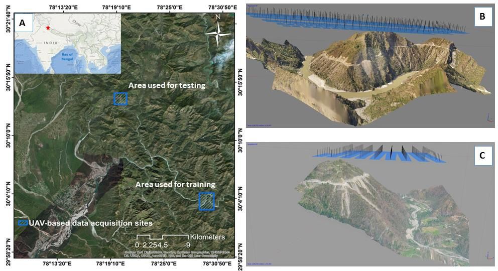
Both the training and testing areas selected for this study were located along the river Ganga, in the Himalayas of northern India (see Figure 1).
This is a high elevation area, with altitudes ranging from 700 m.a.s.l. in the river bed to 2500 m.a.s.l. on the mountain peaks. The rock formations in the area comprise highly fractured and weathered quartzite schist and phyllite [5]. Most of the slope failures occur along the main road, where the road has been widened by cutting into the valley slopes, and they are usually enlarged by heavy rainfall events. This area is therefore particularly vulnerable to mass movements during the monsoon season, when the number of slope failures along this stretch of road is a significant problem. Many new roads are being built at present, to provide access to the numerous popular tourist attractions in the Himalayas [9]. Excavation into slopes for road construction creates areas that are particularly sensitive and susceptible to large mass movements and slope failures. Slope failures along these roads result mainly in debris slides and rockfalls, which block the transportation corridors between the higher Himalayas and the central parts of India. People sometimes have to wait for days for roads to be cleared, as it would be extremely difficult and dangerous to try and get past the road clearance teams on such narrow roads. Slope failures can cause major problems, not only for transportation corridors but also for human settlements, which tend to be located in the lower sections of the roads. Slope failures can have a direct effect on such settlements and have caused casualties in a number of villages.
3. Workflow
3.1. Overall Methodology
The spectral information and the slope data derived from the UAV remotely sensed imagery were used to evaluate the accuracy with which the CNNs were able to detect displaced masses along a road, using different sample patch window sizes. The workflow was as follows:
Layers were first compiled for two different training and testing data sets, one (a) containing spectral information only, and the second (b) containing spectral information and slope data. FAD techniques were used to find the optimal and most detailed slope failure inventories to use for both training and validation purposes. CNN-based patches were created using multiple window sizes. Two different CNN approaches were designed, each with a number of different window sizes. The performance of each CNN approach was tested and validated, and the benefit of and the benefits of including slope data evaluated. A description of the methodology used can be found in the following sections, together with the results of the experiments.
3.2. Materials
UAV Surveys
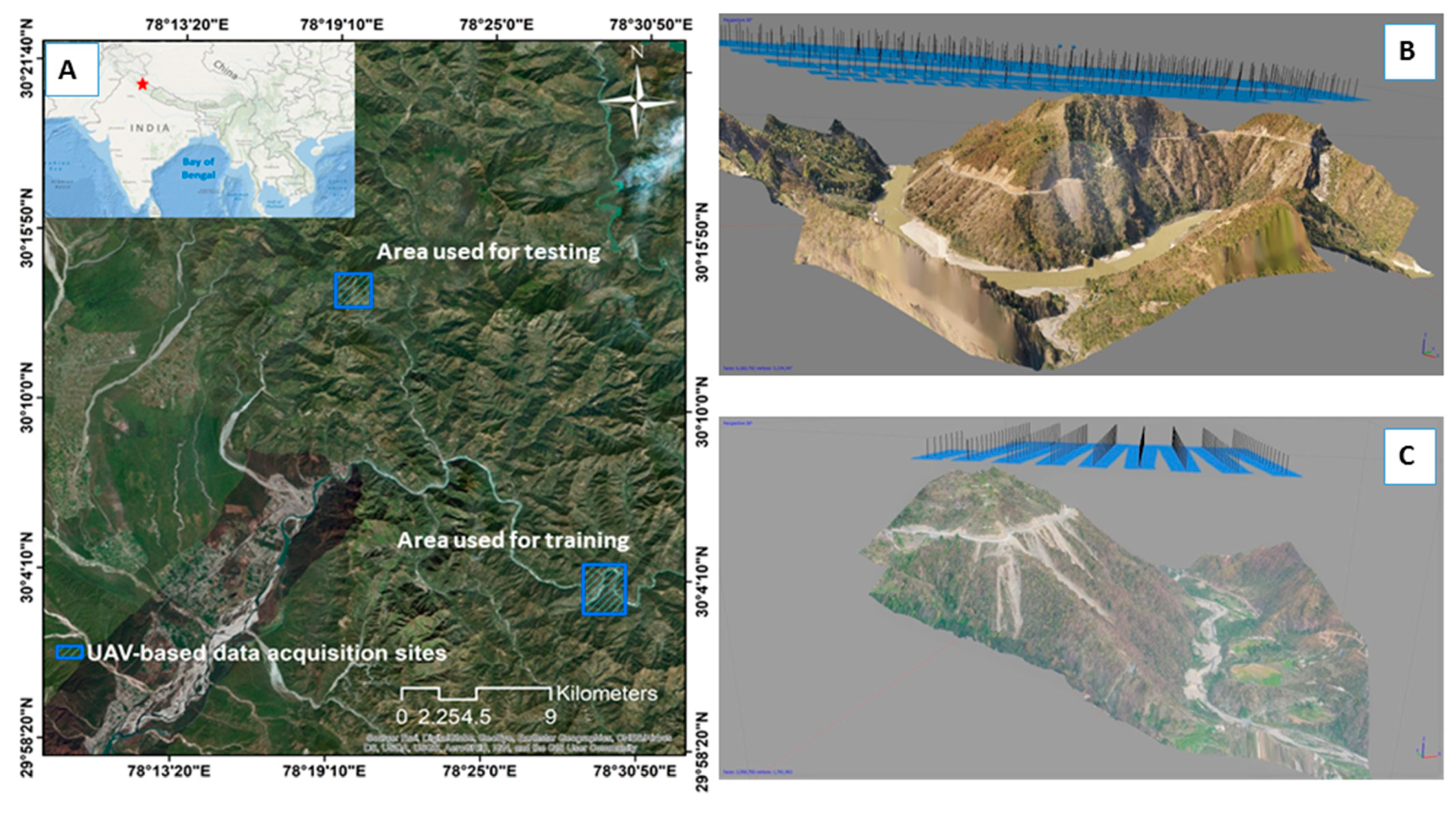
A range of UAVs are currently in use, including both fixed-wing and rotary-wing aircraft. The availability of high quality miniature camera sensors has enabled their use as affordable and practical remote sensing platforms [16]. The low altitude remote sensing platform used for image acquisition in this study (in April 2019) was a quadcopter UAV (DJI Mavic 2 pro, DJI, Nanshan District, Shenzhen, China), see Figure 2), equipped with global navigation satellite system (GNSS), GPS and GLONASS sensors. To achieve acceptable position accuracy with the applied UAV in this study, we used ground control points (GCP) during the fieldwork and data acquisition. Therefore, more than 20 GCPs were measured using GPS (Etre 20X, Garmin, Olathe, Kansas, USA). The accuracy of the GCPs surveyed on the ground is approximately 2 cm standard deviation. The measured GCPs were used in Agisoft Photoscan (St. Petersburg, Russia) during the photo alignment process.
With its 15.4 V/3850 mA-h lithium battery the UAV could fly autonomously for about 25 min following a flight plan, at an altitude of 300 m above the launching site. Data were collected at a ground speed of approximately 15 m/s. An RGB camera was mounted on the UAV and set to collect images at 2-s intervals, which were recorded in a JPEG format. The maximum resolution of the UAV camera was set to 20 megapixel and exposure compensation to -1/3EV. Additional information on the camera is presented in Table 1.
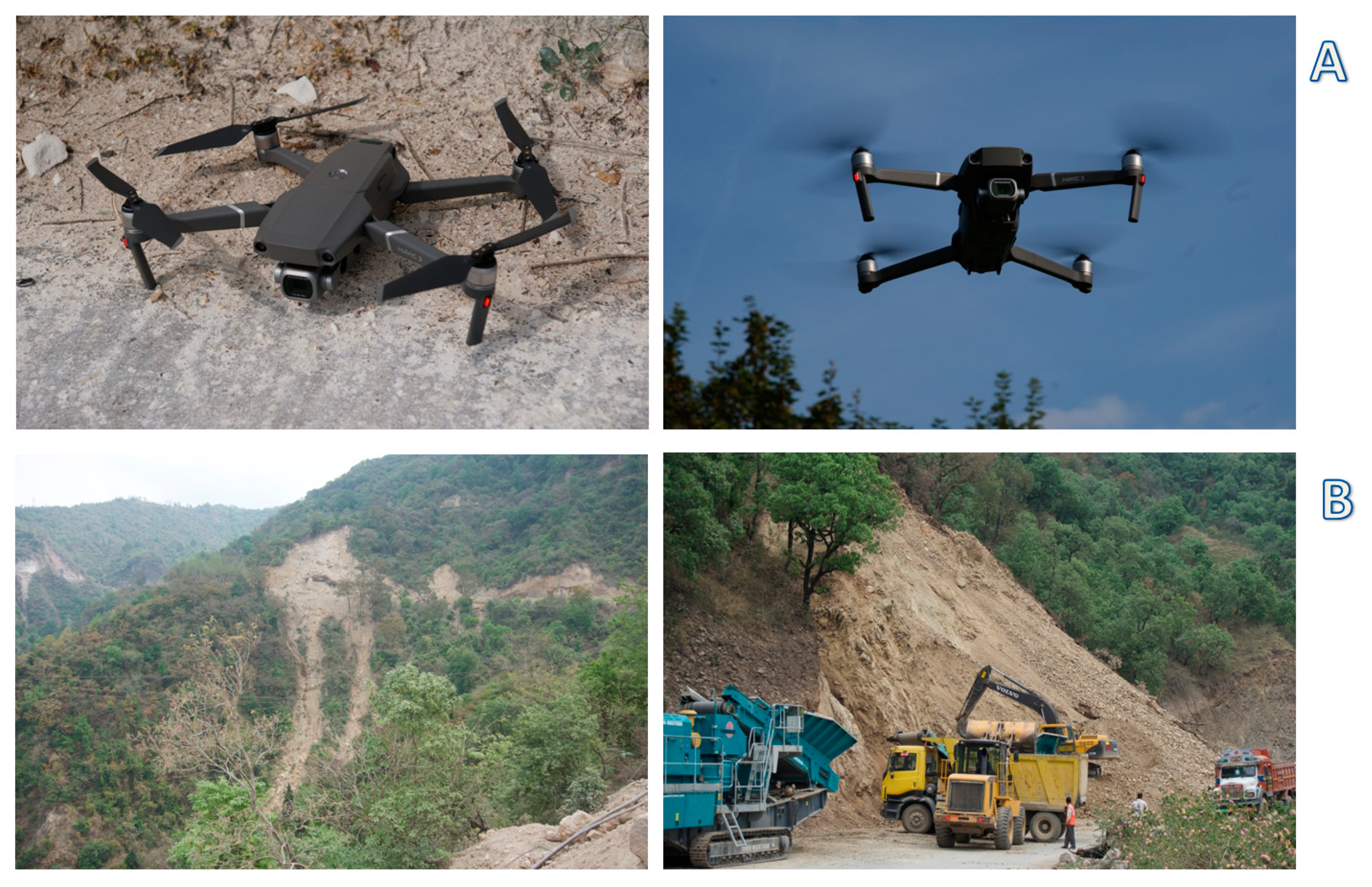
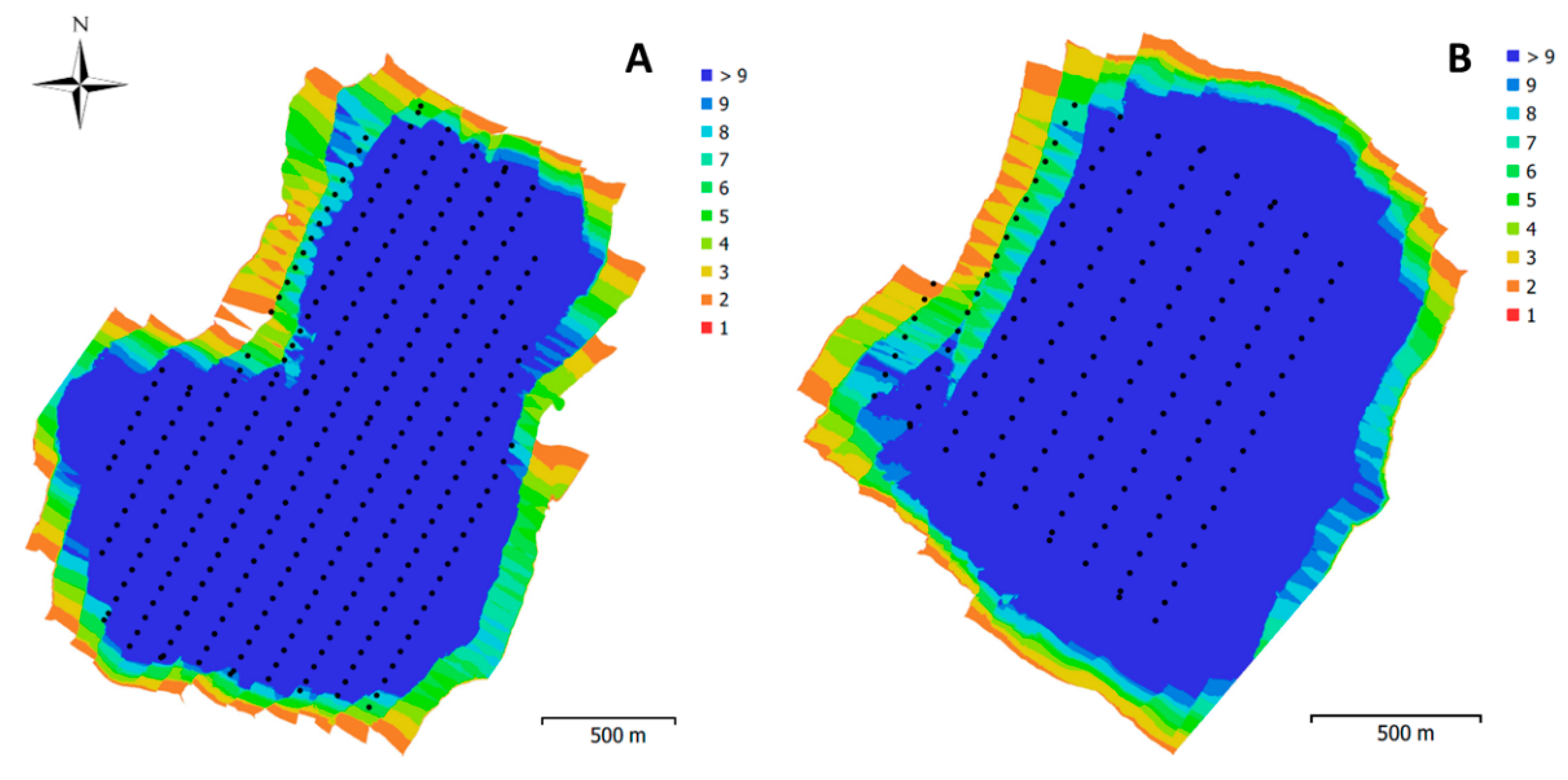
The camera had a 1-inch CMOS sensor with a maximum image resolution of 5472 × 3648 pixels. The camera lens had a focal length of 10.26 mm, resulting in a horizontal field of view (FOV) of 77 degrees. Images were collected during each flight with 75% trajectory overlaps and 65% side overlaps, in order to ensure a high quality for the ortho-mosaic map produced (see Figure 3). RGB images were collected on two flights, one on 8th April 2019 and the second on 9th April; additional information including details of altitude, ground resolution, number of images, and flight dates, can be found in Table 2. A total of 338 images were collected for the training area and 169 for the testing area. The UAV flights were carried out at an altitude of approximately 300m above the launching site. The ground resolution of the imagery obtained over the training and test areas ranged between approximately 11 and 12 cm per pixel. Image overlap between the two study areas ranged from one to more than nine images. The reprojection error is a measure of accuracy of the points, measured in pixels. The reprojection error is one indication of the quality of the calibration process and should be less than or equal to one pixel. According to Table 2, in our case reprojection error is 0.52 pixel for training area and 0.68 for testing area, which are less than one pixel.
3.3. Photogrammetric Processing of UAV Data
Processing of the remotely sensed UAV data started with a manual evaluation of image quality [16]. Those images that had noticeable artefacts or were blurred were deleted, as were those acquired when the drone was too close to the ground (i.e., during take-off and landing). Agisoft PhotoScan software was then used for further photogrammetric processing of the retained images. This processing of raw image data consisted of two steps: (a) ortho-mosaic image generation, and (b) DEM generation.
3.3.1. Ortho-Mosaic Map
To generate a mosaic the acquired UAV image data were processed using software based on the Agisoft PhotoScan Professional 1.5.3 ‘Structure from Motion’ algorithm. Generating the ortho-mosaic images involved three main steps: (a) camera calibration and image alignment, (b) point cloud and mesh generation, and (c) ortho-mosaic map export [30]. The final step generated a map with dimensions of 5472 × 3648 pixels.
3.3.2. Digital Elevation Model Generation
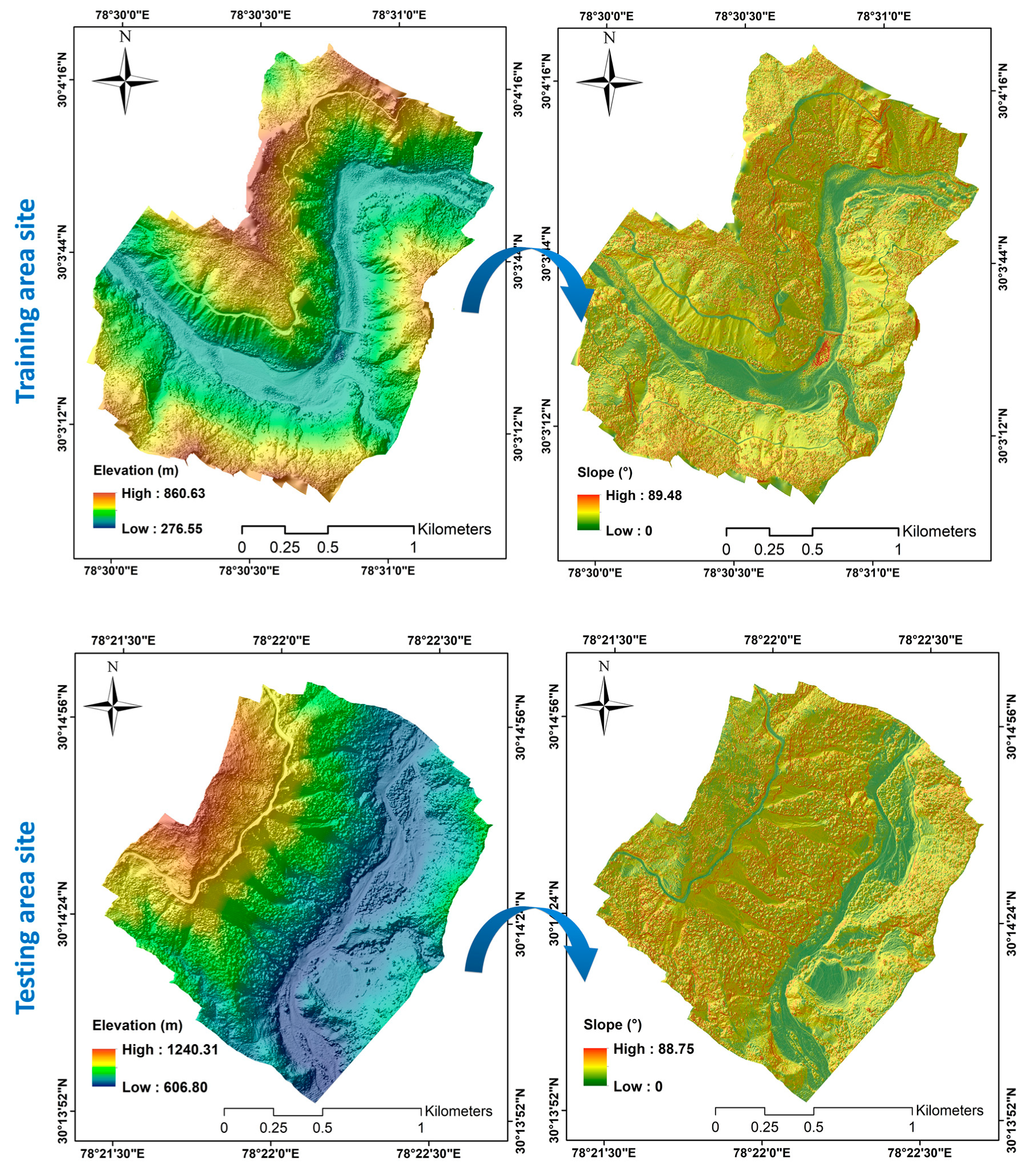
A DEM was produced using the point cloud and mesh generation processes in the same software. A total of 243,141 point cloud points were used for the training area and 121,041 for the testing area. The resultant DEM had a ground resolution of about 44.8 cm/ pixel for the training area and 48.8 cm/ pixel for the testing area. The root-mean-square reprojection error was 0.16 (0.51 pixel) for the training area and 0.12 (0.68 pixel) for the testing area. During the whole the process we were careful to keep the spatial resolution of the orthomosaic resolutions by 11.2 cm/ pixel and 12.2 cm/ pixel for training and testing images respectively. Thus, the resultant DEMs were resampled to the same spatial resolutions. The ortho-mosaic and DEM maps were georeferenced using the latitude and longitude coordinates recorded for each image by the GPS and GLONASS modules on the UAV. The DEMs produced were then used to extract the slope data for both training and testing areas (see Figure 4). The slope data was extracted using ArcMap 10.3 software, (ESRI, Redlands, California, USA).
3.4. Inventory Generation for Training and Testing
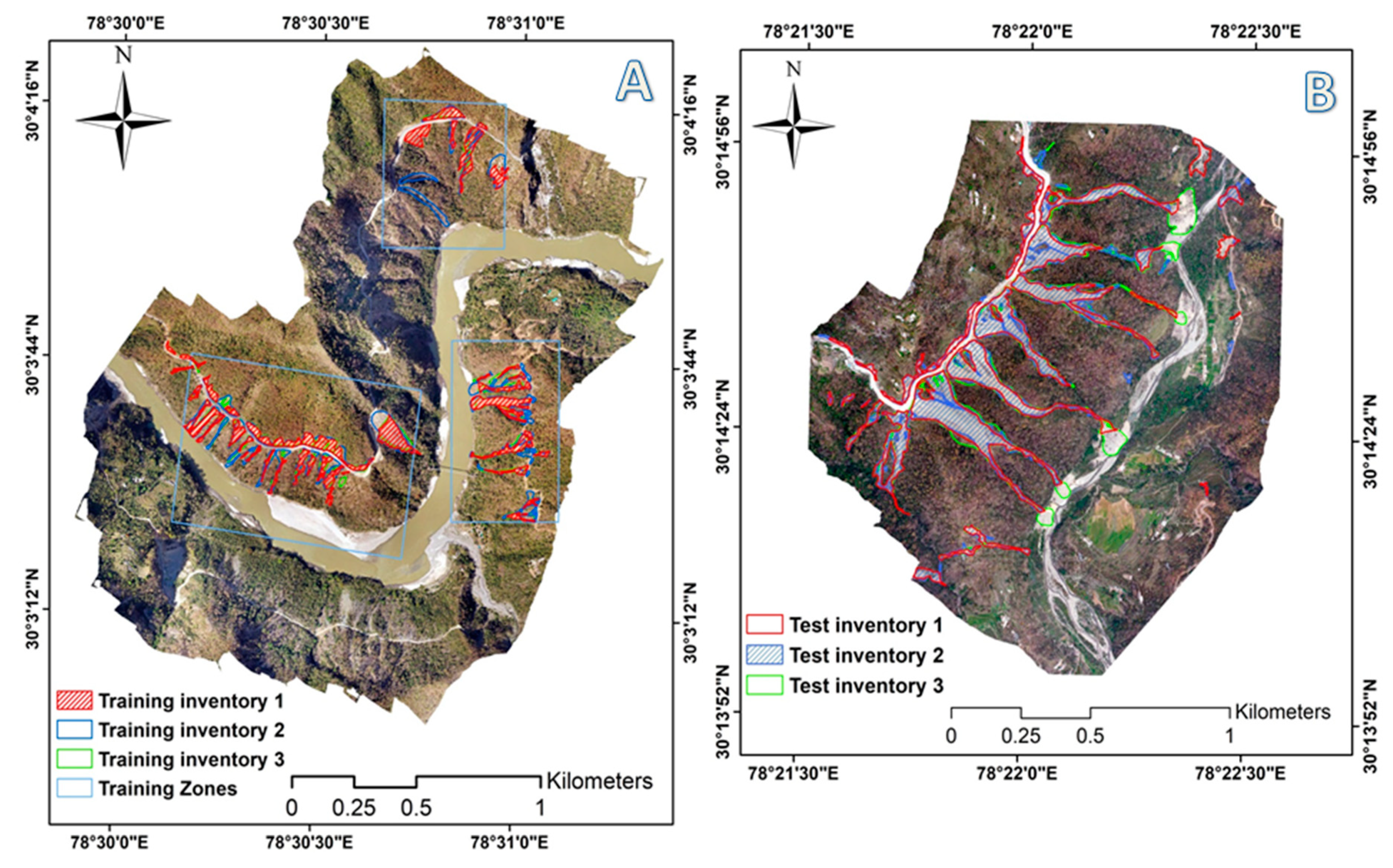
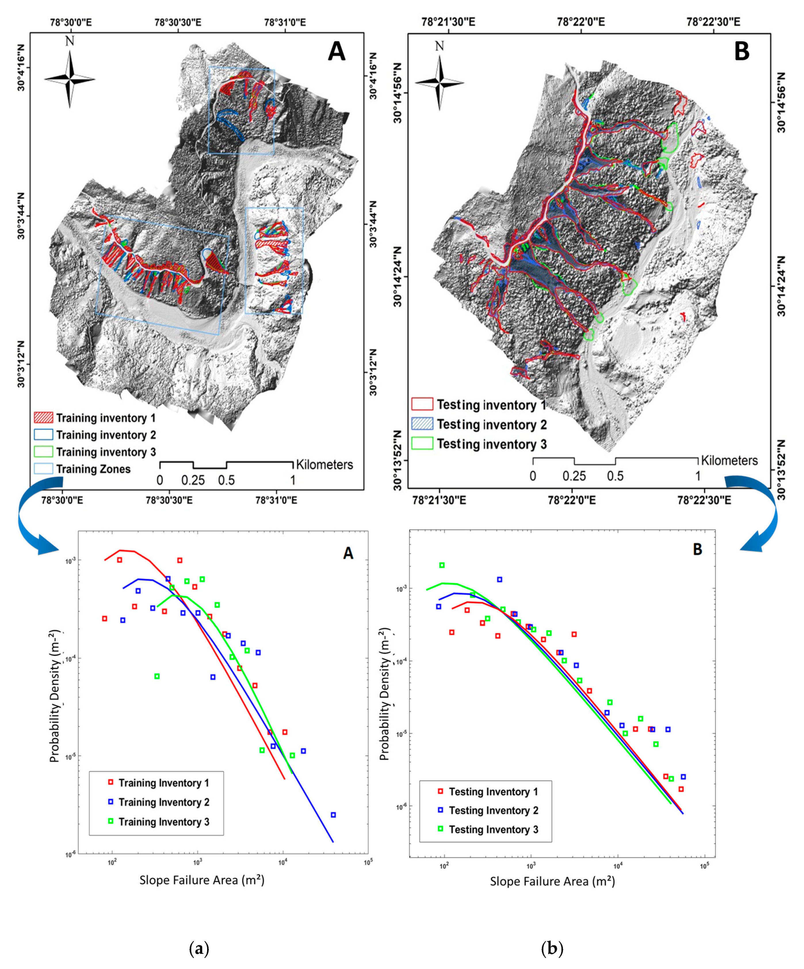
An accurate inventory map of slope failures was required, not only for training the detection algorithm but also for testing its performance. Common techniques used for slope failure inventory production include manual detection and extraction from optical remote sensing data, and field survey techniques such as the use of laser rangefinder binoculars in combination with a GPS receiver. Field surveys are usually expensive and can even be dangerous, and since we had access to very high-resolution imagery we relied on manual slope failure detection from the images that we used for training and testing. Three different experts were asked to manually delineate any slope failures in these images (see Figure 5). A common problem with expert-based techniques is the associated uncertainty in the results [31], which is why three different experts were consulted.
All of the inventories generated by our experts were evaluated using FAD curves. This technique involves plotting areas affected by mass movements against the cumulative and non-cumulative area frequencies. We used a power-law, which is a statistical functional relationship between two quantities. Those areas in the inventories that were affected by slope failures were plotted against their non-cumulative frequency density to generate the FAD curves. The power-law function has previously been successfully used to evaluate some medium to large mass movements [32]. The probability of a landslide of a particular size can be obtained with the power-law using the following equation:
where X is observed values, c is a normalization constant, and β is the power-law exponent of Details of the FAD are presented in Figure 6. In the FAD the power-law distribution curves for larger slope failures diverge from those for smaller slope failures [33]. The point at which this divergence begins is defined as the cut-off point [33]. For non-cumulative probability density distributions of slope failure, the peak value of an FAD curve for small landslides, before it begins to decrease following a positive power-law decay, is referred to as the rollover point [34]. The slope of a power-law distribution is defined by a power-law exponent [35], and that part of the slope that represents large mass movement areas is referred to as the power-law tail. We used this technique to evaluate our inventories, plotting separate FAD curves for inventories for the training and testing areas.
The FAD of the slope failures can be defined by a three-parameter inverse-gamma distribution - see Equation (2) below:
where is the parameter primarily controlling power-law decay for medium and large slope failures is the gamma function of , is the slope failure area, is the location of the rollover point, is the exponential decay for small slope failure areas. According to Malamud et al. [35], the smallest resulting rollover point value is considered to represent the best fit for the power-law exponent.
3.5. Convolutional Neural Network (CNN)
Image processing approaches have traditionally focused on knowledge-based, low-level handcrafted and machine learning feature representations [24]. Although these classification algorithms yield acceptable results for remote sensing classification problems, CNNs have recently been used to obtain state-of-the-art results in computer vision and some limited remote sensing applications (i.e., object detection and scene classification). However, using UAV remotely sensed images for the CNNs still presents a challenge because of the limited availability of labelled data [23]. The multiple layers in feed-forward CNNs are able to provide critical feature representations of an image in a hierarchical manner, which allows them to distinguish the visual laws in the feed-forwarded image from any expert-designed complex ruleset [29]. Any CNN approach involves a number of “hidden” convolutional layers, each consisting of a set of learnable filters together with a nonlinear function, and also pooling layers, which are used to downsample feature maps output from its previous layer in order to reduce computation costs.
The non-linear activation functions commonly used in a convolutional layer are rectified linear units (ReLUs), the sigmoid function, and the hyperbolic tangent function [28]. We used max-pooling, a widely used pooling layer that retains only the maximum values from the feature maps that were produced from its previous convolution layer. The last fully connected layer was responsible for the highly refined features presented in the final probability map [36].
3.5.1. Optimizing Sample Patch Selection
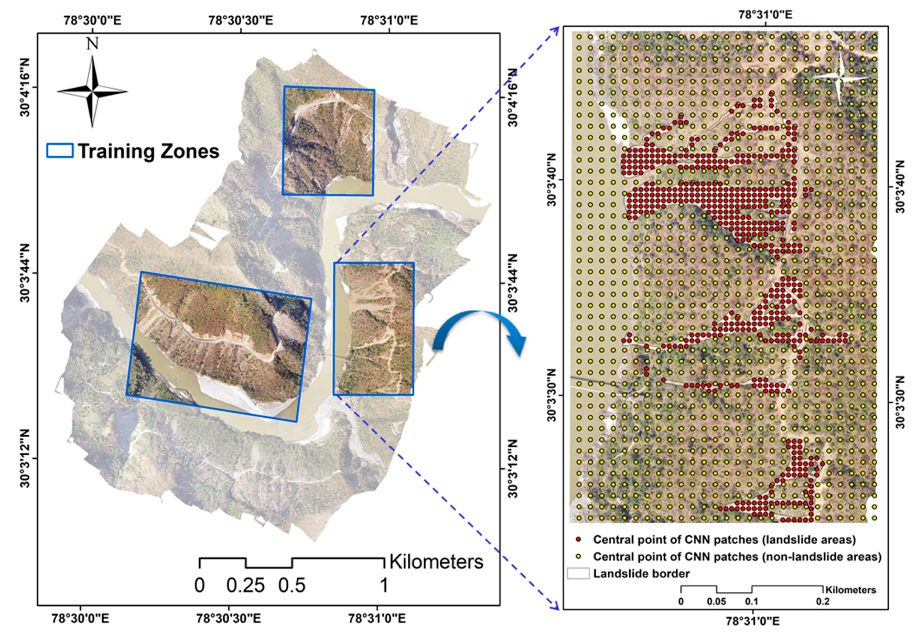
In this subsection the generation of a CNN training data set based on the fishnet tool is explained, and the problems associated with using the common sample patch selection methods (such as the random, central, and moment bounding (MB) box methods) for our specific purpose of slope failure detection discussed. The ultimate objective of preparing any CNN training dataset is to obtain a consistent set of sample patches for feature extraction, segmentation, and object detection [37]. The method most commonly used to select patches is the random selection method, which has been used in a number of previous investigations [28,38]. The MB box method has also been used and is considered a practical method for finding both the optimal position and the optimal size for the patches. The advantages of using the MB box method for CNN sample patch selection have been previously described by Zhang et al. [39], in an investigation into the use of object-based CNN for urban land use classification. However, in view of the large variation in the shape and dimensions of areas affected by slope failure, using this detection method leads to a large increase in the number of neighboring areas in each patch, resulting in increased computation time and reduced accuracy. The central sample patch selection method has been proposed by Ghorbanzadeh and Blaschke [40], who used only those patches selected from the central line/point of an object and compared their results with those obtained using random selection. They found that using the central patch selection method increased the accuracy by 3%. However, considering the resolution of our VHR images and the applied window sizes for sample patches selection, this method is not applicable to our case. We therefore used the fishnet tool, which provides us with equally spaced points that were considered as the central point of each patch. The fishnet tool was used on the inventory polygons in the UAV image that was selected for training (see Figure 7). The central points of the sample patches were then selected on the basis of the fishnet points. Based on the ratio of the slope failure areas to the non-slope failure areas in the images, different distances were applied for the fishnet points. Thereafter these points were used for patch selecting from the slope failure inventory polygons and the other areas.
3.5.2. CNNs with Different Patch Window Sizes and Network Depths
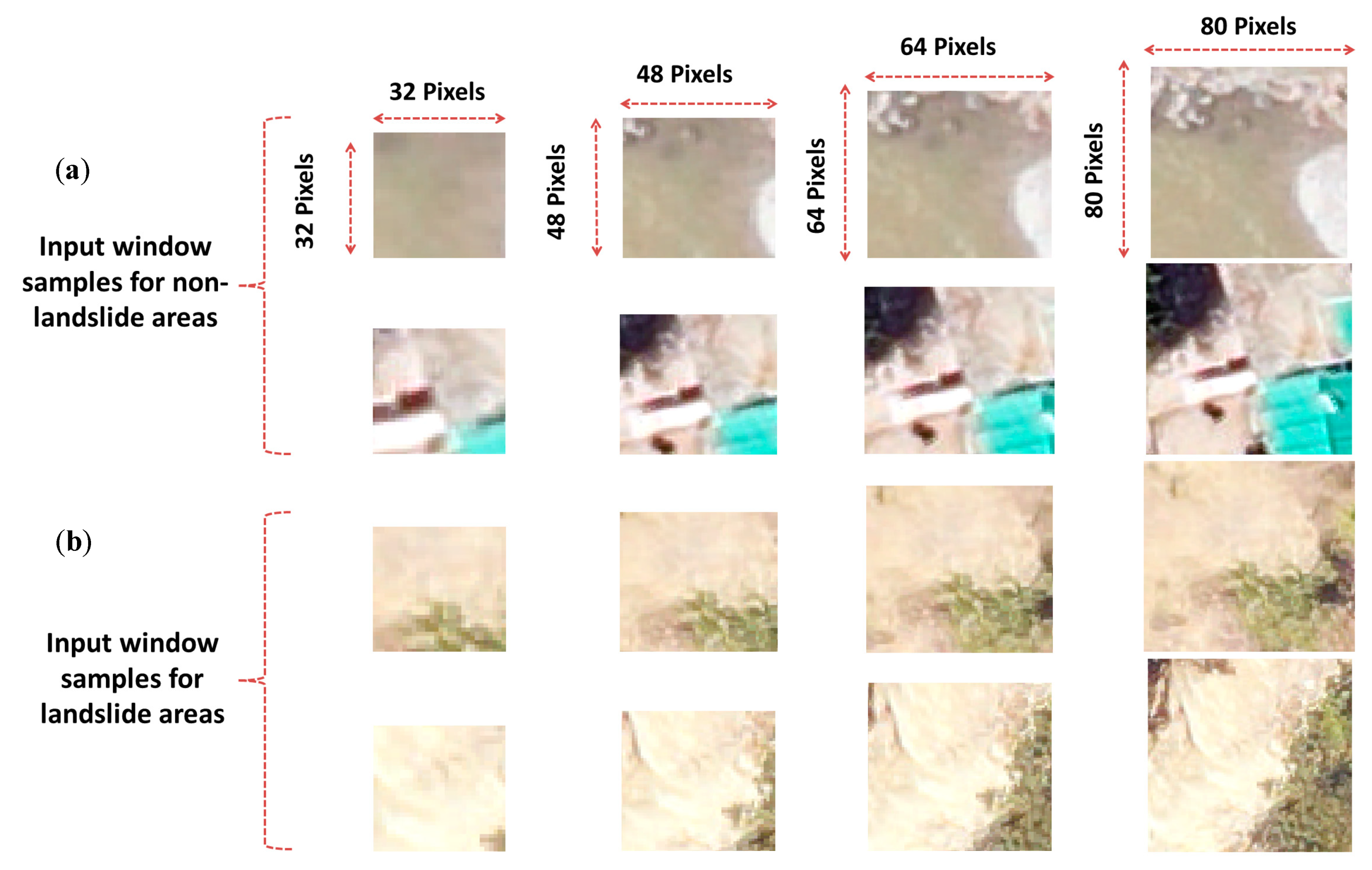
We used multiple CNN training window sizes for slope failure detection. Four sample patch window sizes (32 × 32, 48 × 48, 64 × 64, and 80 × 80 pixels) were used for the CNN training windows. These CNN training window sizes were carefully chosen on the basis of cross-validation results. Multiple input window sizes were used because of the extent of the inventory polygons and the different dimensions of the slope failures. Most of the slope failures were quite extensive along the line of failure, becoming narrower below this line before broadening again in the depositional area. The resulting features can therefore sometimes be quite elongated and thin, more closely resembling an unsealed road than a mass movement. However, we also used the slope data and a single slope failure can consist of different slopes, which should be taken into account in the training process. Zhang et al. [39] and Ghorbanzadeh et al. [28] have previously used the same approach in separate studies to annotate sophisticated shape features in urban areas and in slope failure areas.
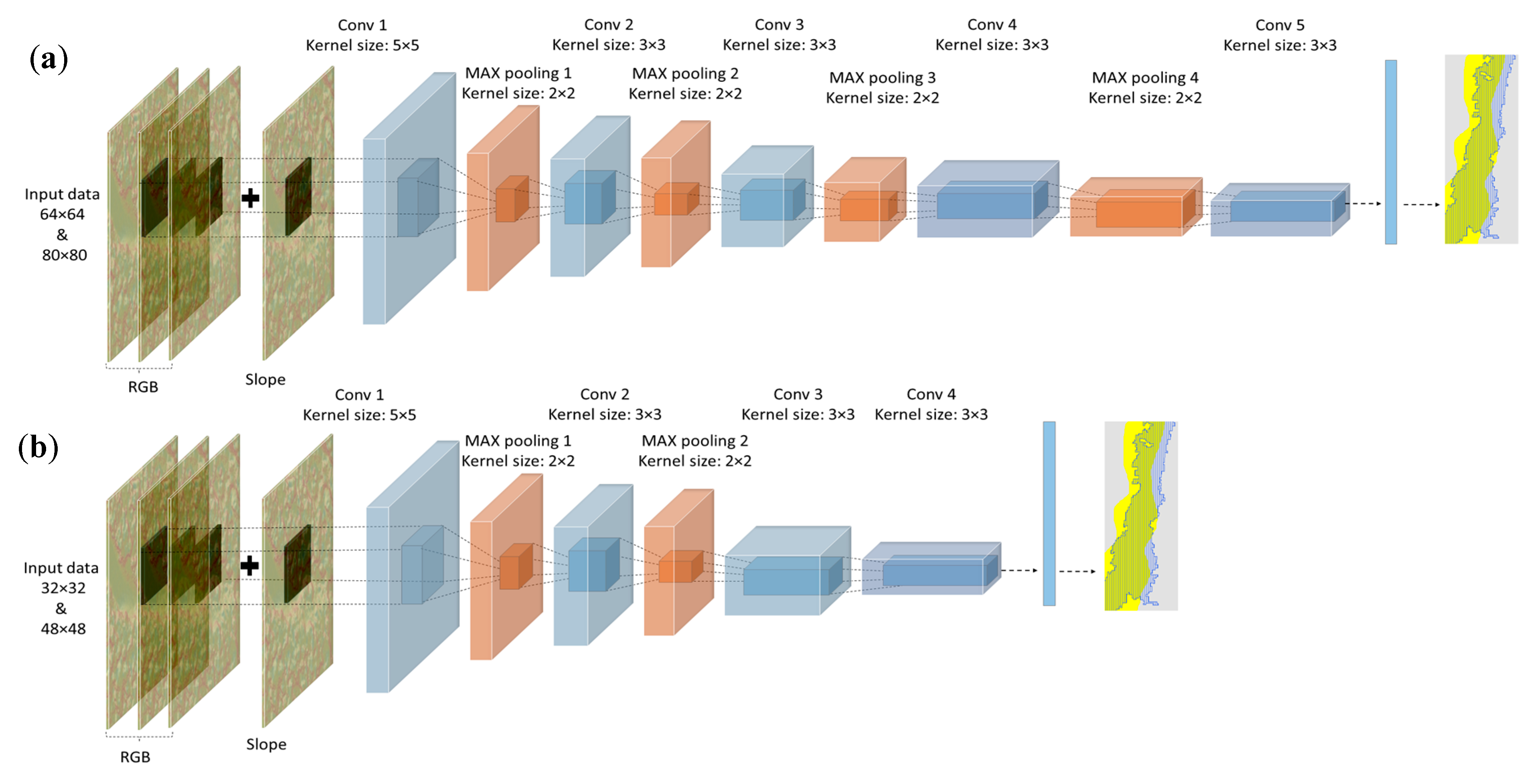
Automatic frameworks for designing the state-of-the-art CNN architectures without any expert knowledge have considered as a crucial part of the related studies recently [41]. There are some studies that attempt to find an automatic solution for defining the optimized CNN architectures [42,43]. However, these frameworks have automatically optimized based on their specific applied training datasets such as CIFAR-100, MNIST, and Tiny-ImageNet, whereas in our case we use our prepared training dataset using the multiple input sample patch selection window sizes. Although the optimal architecture for any specific application of a CNN approach remains a matter of ongoing discussion [44], the number of convolution and pooling layers should correspond to the input patch window sizes. In this study, the number of hidden layers including the convolution and pooling layers is defined by term “depth” taken from term “deep” of deep learning which refers to the several hidden layers in a neural network. We used two CNN structures with a different number of layers in each, in response to the multiple input window sizes that we used (see Figure 8). A six-layer depth CNN was used for 32 × 32 pixels and 48 × 48 pixels window sizes, and a nine-layer depth CNN for 64 × 64 pixels and 80 × 80 pixels window sizes. Both CNNs were fed with the three original RGB spectral bands of the UAV remotely sensed image. We then added the slope data to the input data set as an additional layer. A composite of four layers was therefore used for training both of the CNNs. We used different numbers of feature maps and a max-pooling layer of 2 × 2 was applied immediately after any convolution layer except the last layer of the six-layer depth CNN. The dimensionality-reduced feature maps of the max-pooling layer were then used as input for the next convolution layer. A kernel size of 5 was used for the first convolution layer and of 3 for additional convolution layers. Using a dropout of 0.5 is useful for fully connected layers to increase the generalization of the approach and avoid overfitting, which result in better transferability of the approach. Dropout is considered as a regularization method which use during training and it randomly dropped the connections among the network for reducing overfitting [23]. The kernel sizes and the number of feature maps were selected on the basis of our input window sizes. The last convolution layer of the six-layer depth CNN and the last max-pooling layer of the nine-layer depth CNN were not used for the 32 × 32 and 64 × 64 pixels window sizes, respectively, due to the dimensionality limitation. Our CNN approaches were structured and implemented in Trimble’s eCognition software, based on the Google TensorFlow software library. The resulting gradients for each weighting were calculated within each hidden layer, and a statistical gradient descent function applied to optimize these weightings. The best detection rate was obtained with a batch size of 50, a learning rate of 0.0001, and 5000 training steps.
4. Results
4.1. Selection of Optimal Inventories
The FAD curves were plotted for each of the training and testing areas (see Figure 9) and the extracted values are presented in Table 3. The minimum slope failure areas extracted for the training area ranged between 81 m2 for the first inventory and 334 m2 for the third inventory; those extracted for the testing area ranged between 86 m2 for the third inventory and 144 m2 for the second. The β value ranged from 1.44 to 148 for the training inventories and from 1.53 to 2.02 for the testing inventories. The smallest rollover point value for the training inventories was 256.74 m2 for the first testing inventory, while the smallest rollover point value for the second testing inventory was 171.31 m2. The first inventory for the training area and the second inventory for the testing area were therefore selected as our optimal inventories and used for the training and testing approaches. From the resulting rollover point values we can not claim that the selected inventories are the most accurate, but we can say that the distribution patterns obtained from these inventories were closest to those of accurate slope failure inventories.
The first inventory for the training area, which included three different zones, was the one used to train the different CNN approaches. The fishnet tool was used to produce point features on a uniform grid, based on the inventories for the training zones. The points produced were taken to be the central points of CNN sample patches. The distribution of the sample patches was therefore based on the fishnet tool. As the total area covered by slope failures within a particular image was less than the total area unaffected by slope failure and almost the same number of points allocated to slope failure areas as to areas unaffected by slope failure, the distance between points created within the slope failure areas was less than that between points created outside the slope failure areas.
This higher point density within the slope failure areas made up for their smaller area, resulting in a balance between the total number of points within slope failure areas and the number outside these areas. This balance within the CNN training data is crucial and needs to be taken into account in the training process [28]. Sample patches were generated for all windows with 32 × 32, 48 × 48, 64 × 64 and 80 × 80 pixel sizes, based on the fishnet points. An illustration of sample patches generated for different window sizes is presented in Figure 10.
4.2. Results of Slope Failure Detection
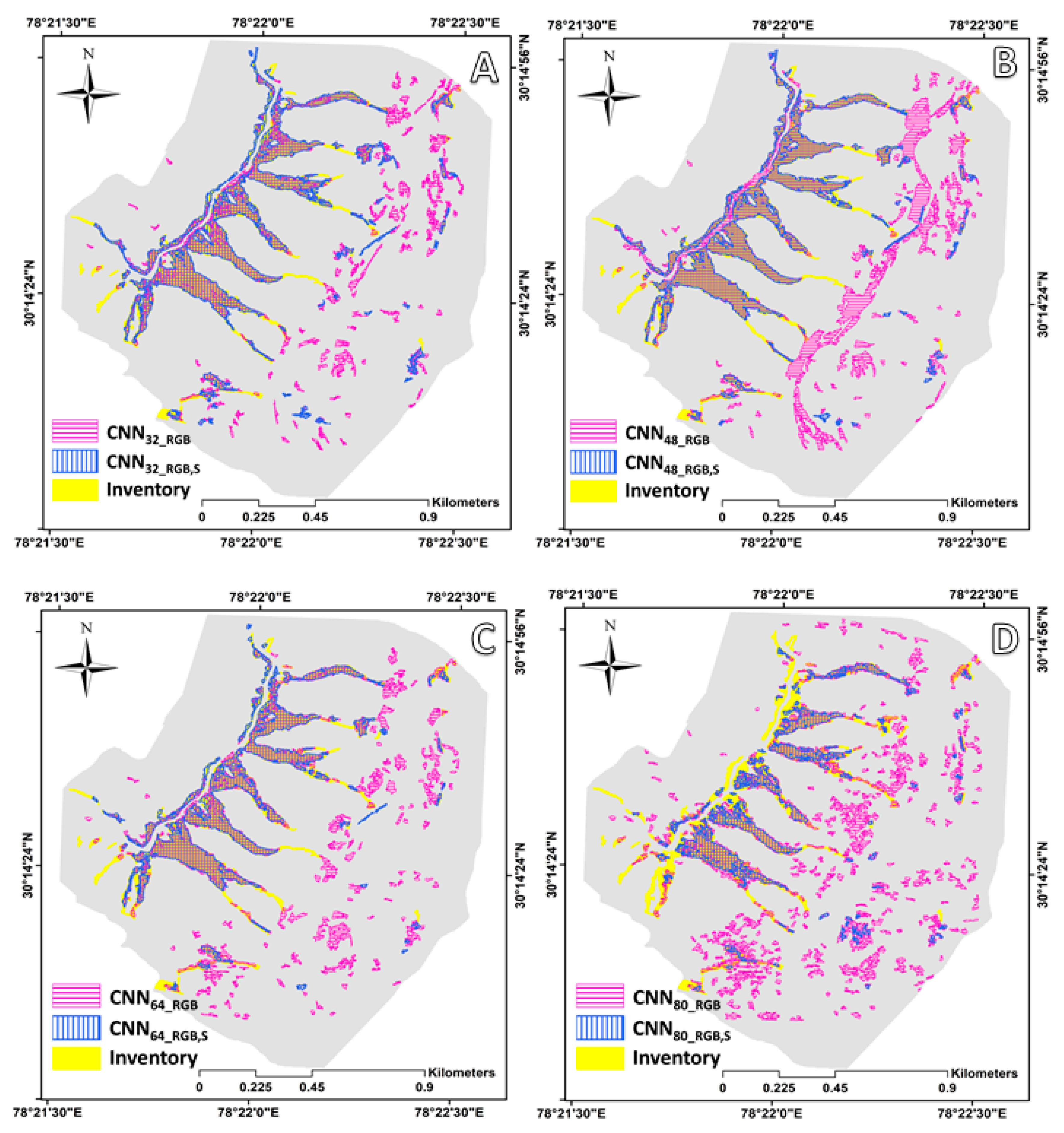
The CNN approaches using all of the above-mentioned parameters were trained using the selected inventory data set for the training zones and tested on the testing area. In all of the resulting maps we removed those detected slope failure areas that covered less than 144 m2 in order to reduce the geometric inaccuracies between the inventories and the UAV remotely sensed images. This area was the area of the smallest polygon in the inventory map chosen for the testing process. The results of a statistical analysis of the detected slope failures (i.e., minimum, maximum, sum, mean and standard deviation of the extracted areas) are presented in Table 4. A total of eight slope failure maps were generated on the basis of all the different CNN approaches and parameters used. Each of the presented maps (see Figure 11) shows the results obtained using the same sample patch window size with different RGB and RGB,S (RGB and slope) data sets, making it easier to distinguish the effects of using different training data sets and sample patches. Both results were overlaid on the chosen optimal testing inventory map. As an example, the approach used a window size of 48 × 48, and RGB,S indicates the use of a training data set comprising optical data from RGB layers, together with slope data.
5. Comparison of Results Obtained by Manual Detection with Those Obtained Using CNNs
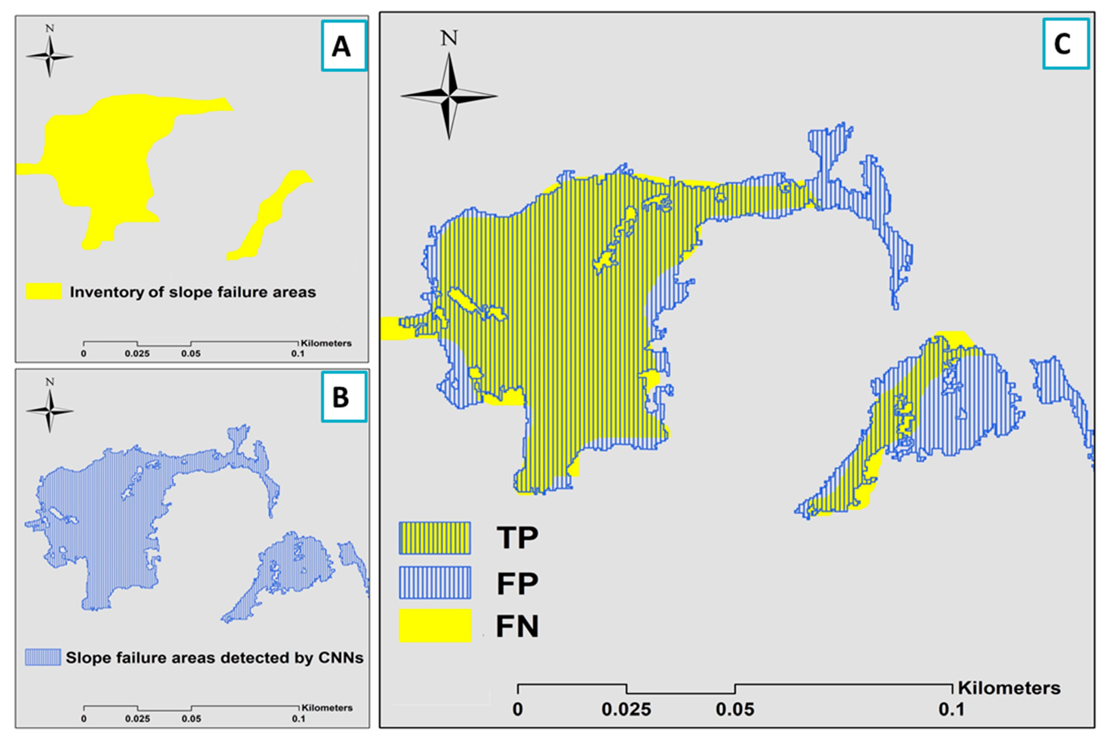
A number of accuracy assessment measures relevant to this study were used to comprehensively evaluate the performance of the applied CNNs by analyzing the conformity between the manually detected slope failure inventory dataset and the dataset derived using CNNs. The performances were compared using the positive predictive value (PPV), the true positive rate (TPR) and the F-score metrics. These accuracy assessment measures were calculated using three different pixel classifications: true positive (TP), false positive (FP), and false negative (FN) - see Table 5. The PPV, also known as the precision (Prec) [45], the proportion of slope failure pixels correctly identified by the CNNs, which can be calculated as:
where TP is the number of pixels that were correctly detected as slope failure areas (i.e., the number of true positives) and FP is the number of false positives – i.e., pixels that were incorrectly identified as slope failure areas (see Figure 12).
The true positive rate (TPR), also known as the recall (Rec), is the proportion of slope failure pixels in the polygons extracted manually from the slope failure inventory that were correctly detected by the CNNs, which is derived as follows:
in which FN is the number of inventory slope failure areas that were not detected by the CNNs, i.e., the number of slope failure areas missed (see Figure 12). The F-score was used to reach an overall model accuracy assessment. The F-score, also known as the F1 measure (F1), is defined as the weighted harmonic mean of the PPV and the TPR, which is calculated using Equation (5):
where α is a figure used to define the desired balance between the PPV and the TPR. When α= 0.5, the PPV and the TPR are in balance, a compromise that gave the highest level of accuracy in our CNN results. The over prediction rate (OPR) - also known as the commission error, the unpredicted presence rate (UPR) [46], are the other relevant accuracy assessment measures used to assess the similarity between manually extracted slope failure areas and CNN-detected areas. These measures are also based on matches and mismatches between the inventory and the CNN-detected polygons of slope failure areas using TPs, FPs and FNs, which can be estimated using Equations (6) and (7):
The mean intersection-over-union (mIOU) is another accuracy assessment metric that applied in this study. The mIOU is a known accuracy assessment metric in computer vision domain, particularly for semantic segmentation and object detection studies. The application of mIOU for landslide detection validation is fully described by [28] and [40]. In general, the mIOU is an appropriate accuracy assessment metric where any approach that results in bounding polygons (see Figure 13) can be validated by using this metric based on the ground truth dataset. It is specified as the mean of Equation (8):
The approach achieved the highest overall accuracy assessment, with an F-score of 85.46%, followed by the and approaches which achieved F-scores of 80.67 and 79.42%, respectively (see Table 6).
The and approaches resulted in the lowest F-scores, both having values of just over 59%. All CNNs apart from those that used a sample patch size of 80 × 80 pixels, yielded higher F-scores when the slope data was taken into account in the training and testing processes. The greatest increase in accuracy obtained by including the slope data was in the CNN with a sample patch size of 48 × 48 pixels, whose F-score increased by 2%; the mIOU value of results from the same CNN when including the slope data increased by about 35. The increases for CNNs with sample patch sizes of 32 × 32 and 64 × 64 pixels were smaller, at about 18 and 19 percent, respectively. The PPV for was 83%, whereas that for was 89.9%; their TPR values decreased to 78.46% and 81.85%, respectively.
6. Discussion
6.1. Sample Patch Selection and Optimality in CNNs
Recent publications have reported high classification performance for CNNs, particularly when compared to the traditional machine learning classifiers. We have also achieved good results with CNNs but our research has shown that it is critical to select appropriate CNN sample patch window sizes and input training data for the specific area under investigation. Sample patch window sizes need to be defined that best reflect the resolution of the images, the dimensions of the areas affected by slope failure, and the shape complexity of the features in the study area. This is often achieved by trial and error and it remains unclear if the window size that yields the highest accuracy in one study will also yield the best results when used in other studies. However, the parameters used in our approach can certainly be used for other similar areas in the Himalayas, when using UAV images with a similar resolution.
There are a number of different ways to design a CNN approach. As discussed in the Introduction, a CNN will not automatically outperform other classification algorithms and feature extraction models, in spite of any such claims in popular science articles. Furthermore, using different training data for the same CNN approach can have a significant effect on the slope failure detection results.
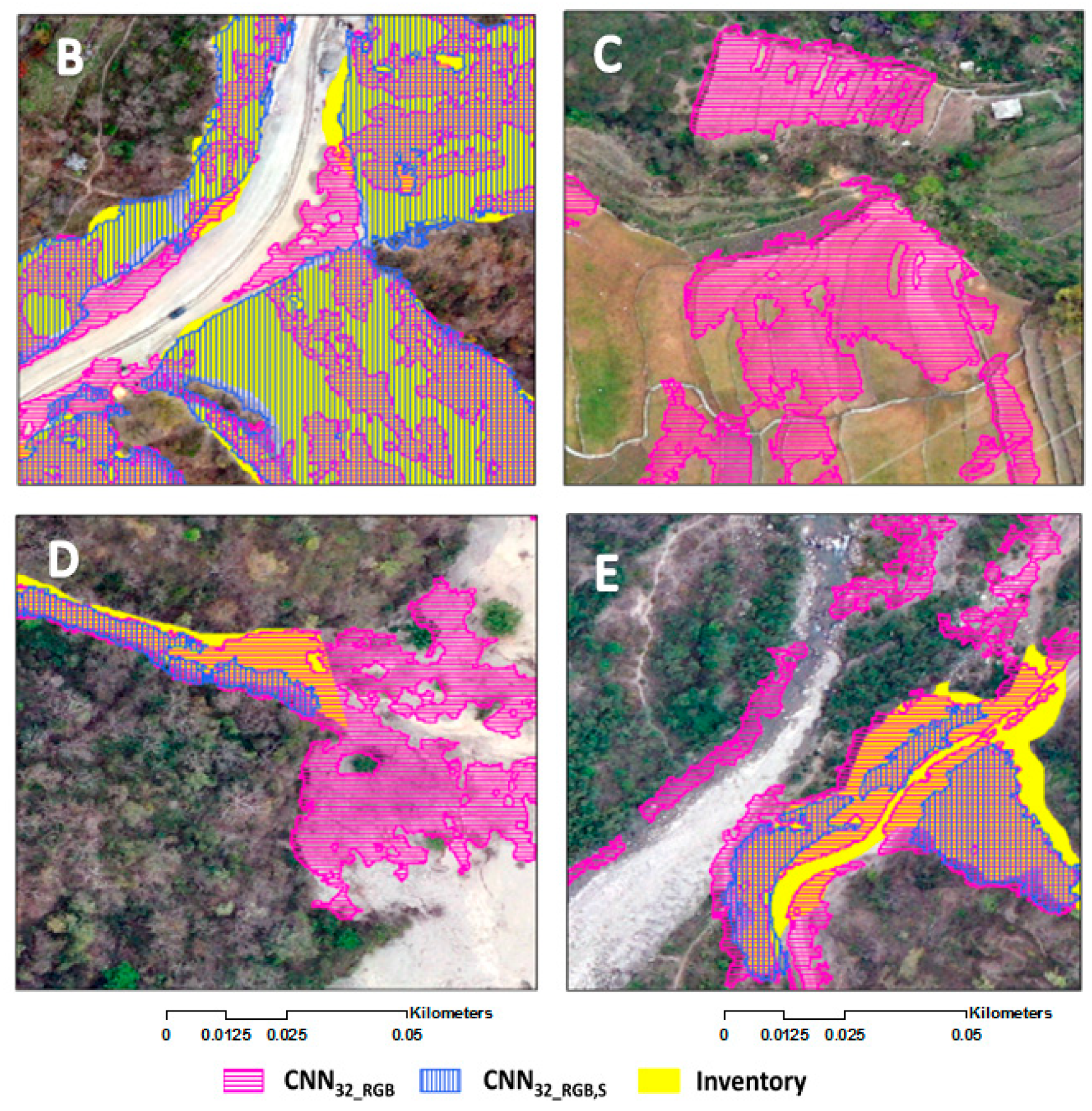
Our experiments have shown that similarities between slope failures and other neighboring features can result in an increased number of FPs. In both of our study areas woodlands were the most common areas adjacent to slope failures. As our CNN approaches were trained with sample patches that took into account these neighboring areas within the window, it was possible to select those areas neighboring to any woodland as the slope failure. This problem is illustrated in Figure 14E: most of the river bed areas adjacent to woodland were incorrectly identified as slope failures, increasing the number of FPs. This problem even is much more when the slope was also applied for training the CNNs and because the samples contain much more neighbored areas with different slope degrees. This is the reason that, as the sample patch window size increases, the overall detection accuracy decreases. As the window size increases, the amount of information that it contains on those areas with no slope failures will also increase if the window is located close to the edge of an area affected by slope failure. Thus when we used a window size of 80 × 80 pixels we obtained the lowest accuracies in almost all accuracy assessment metrics (except the PPV, which yielded a value of 0.86). The mentioned patches could be easily removed by selecting the border areas of an area affected by slope failure. However, this would result in information on the exact position of the border of the area affected by slope failure being lost. A balance therefore needs to be found between the amount of information required from those areas with no slope failures and from the slope failure itself.
However, using small window sizes results in having less information from those areas with no slope failures while still retaining critical information from the border areas of slope failures within the window. By reducing the window size, useful information on the neighboring areas and on the shape a patch, as well as spectral information, would be lost. A CNN approach with a window size of 48×48 pixels yielded a higher F-score when using both input data sets than an approach using a smaller window size of 32 × 32 pixels.
6.2. UAV Remotely Sensed Multiple Training Data Sets
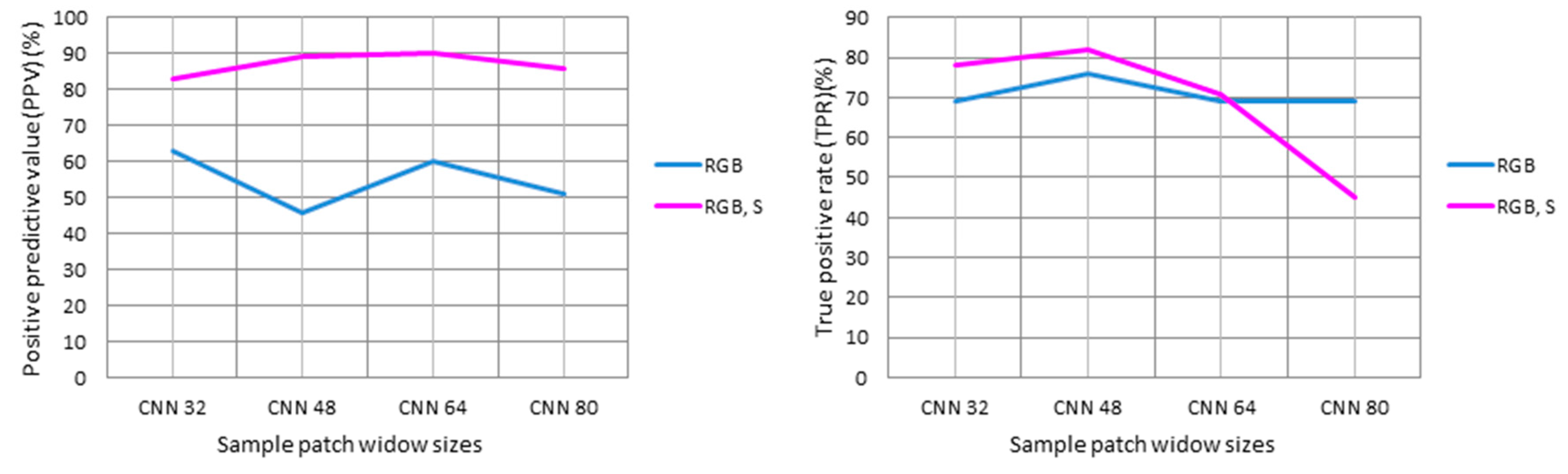
For our research we used two different training data set composites, different sample patch window sizes, and multiple-layer depth CNNs. The only spectral information that we used was derived from the UAV remotely sensed images. According to the different accuracy assessment metrics used in this study, using only optical data resulted in a larger number of FPs than using a combination of optical data and slope data. Similarities between the spectral information from areas affected by slope failure and spectral information from the wrongly detected areas was the main reason for the increase in the number of FPs. Most of the river bed areas (see Figure 14D,E), the road sections (see Figure 14A,B), and uncultivated agriculture fields or bare soils (see Figure 15), usually yielded similar spectral information to areas affected by slope failure. We concluded that, within our study area, it is necessary to use high-resolution slope data for efficient slope failure detection, as it helps to distinguish between different features with similar spectral information within areas affected by slope failure. Using multiple training data sets derived from UAV remotely sensed images, together with different sample patch window sizes, is a practical way to determine the influence of each parameter on the accuracy of slope failure detection. The PPVs levelled out at around 0.85 when the CNNs with different window sizes were trained using the RGB optical data in conjunction with the slope data (see Figure 15). However, the PPV fluctuated around 0.55 when the same CNNs were trained with only the optical RGB data. Use of the slope data therefore reduced the effect of using different sample patch window sizes and, more importantly, resulted in a significant increase in the PPV of the results. The increase in PPV varies as the parameters vary. Although using the RGB data set yielded almost identical TPR values for different window sizes (see Figure 15), using the data set that combines RGB data with slope data dramatically reduced the TPR value when the window size was increased.
6.3. Limitations of This Research
Slope failures have traditionally been detected using knowledge-based algorithms or by visual interpretation of satellite images. The availability of VHR imagery facilitates visual interpretation of slope failures but the requirement for rapid updating of slope failure maps makes an automated approach essential. Our approach has its restrictions because of limitations in our UAV image acquisition, for example in the number of images acquired and the number of spectral bands available. Since only one set of images was acquired for both training and testing areas we were unable to obtain any mass displacement information, since that would require two or more different DEMs. Displacement information would be useful for illustrating the differences between stable areas and areas of slope failure at a specific point in time. The camera used was also unable to capture the near-infrared (NIR) band.
There are also some general limitations regarding the use of UAVs. The market for drones is growing rapidly due to rapidly improving hardware and software, and they have many uses, including field surveys. However, they still have a number of problems such as the limited battery life, which is the main factor preventing larger areas being covered without requiring interim landings and battery replacement before restarting. The limited availability of GNSS satellites is another problem with using UAVs, and wind conditions can also lead to complications, mainly in mountainous areas [47]. Despite these limitations, UAVs are considered to be quite flexible and a valuable tool for monitoring slope failures. We have confirmed the value of using UAV remotely sensed images with CNNs for slope failure detection (when using appropriate parameters), as has been previously reported [12]. However, choosing the optimal parameters when designing a CNN network, including the optimal CNN design and depth, the training data set, sample patch selection, and the training data set, in order to obtain the best results, remains problematic. The presented work offers some solutions to these problems, although these solutions still require improvement as the best options were selected on the basis of trial and error and cross-validation.
7. Conclusions
We have investigated the effectiveness of CNN approaches based on UAV remotely sensed images for slope failure detection. The increasing availability of VHR imagery from different sources, such as UAV products, provides many options for detecting and mapping mass movements. The detection of slope failures that occur along road networks remains a challenging task due to the complexity of possible triggering factors and the many shapes and sizes that the associated mass movements can have. We have analyzed and compared different CNN approaches for slope failure detection along road networks in the Himalayas, using different training data sets and parameters. As could be expected, the CNN approach that included slope data yielded the highest detection accuracy. We conclude that CNN approaches have a high potential for mass movement detection. However, CNNs are currently designed by trial and error and it often remains unclear why a particular design yields the highest accuracy. CNN approaches generally require little human supervision compared to more traditional approaches, and they can be easily transferred to other regions by retraining the CNN with new training data. However, the effectiveness of such approaches for slope failure detection when reapplied at a larger scale remains unclear. Our future work will aim to develop an object-based CNN approach for the detection of different types of slope failures such as debris slide and rock fall. We will aim to increase the detection accuracy by combining CNN productions with object-based geographic analysis. We also plan to investigate a linear transformation method for data augmentation as an alternative to the data distortion methods that have recently been widely used, which are based on deformation techniques used to artificially multiply the volume of the training data set. We thus hope to enable CNNs to reach their full potential in image classification, to move beyond the more standard tasks of basic feature identification in imagery, and to deal with the various problems associated with remotely sensed imagery such as terrain effects, shadows, variations in radiometric conditions, etc.
Author Contributions
Conceptualization, O.G.; methodology, O.G., and S.R.M.; software, O.G., and S.R.M.; validation, O.G. and S.R.M.; data curation, S.R.M.; writing—original draft preparation, O.G. and S.R.M.; writing—review and editing, T.B., and J.A.; visualization, O.G. and S.R.M.; supervision, T.B. and J.A.; funding acquisition, T.B. All authors read and approved the final manuscript.
Funding
This research is partly funded by the Open Access Funding of Austrian Science Fund (FWF) through the GIScience Doctoral College (DK W 1237-N23).
Acknowledgments
We would like to thank four anonymous reviewers for their valuable comments. Open Access Funding by the Austrian Science Fund (FWF).
Conflicts of Interest
The authors declare no conflict of interest.
References
- Sarro, R.; Riquelme, A.; García-Davalillo, J.C.; Mateos, R.M.; Tomás, R.; Pastor, J.L.; Cano, M.; Herrera, G. Rockfall simulation based on uav photogrammetry data obtained during an emergency declaration: Application at a cultural heritage site. Remote Sens. 2018, 10, 1923. [Google Scholar] [CrossRef]
- Miura, H. Fusion analysis of optical satellite images and digital elevation model for quantifying volume in debris flow disaster. Remote Sens. 2019, 11, 1096. [Google Scholar] [CrossRef]
- Pourghasemi, H.R.; Rahmati, O. Prediction of the landslide susceptibility: Which algorithm, which precision? Catena 2018, 162, 177–192. [Google Scholar] [CrossRef]
- Watson, C.S.; Kargel, J.S.; Tiruwa, B. Uav-derived himalayan topography: Hazard assessments and comparison with global dem products. Drones 2019, 3, 18. [Google Scholar] [CrossRef]
- Meena, S.R.; Mishra, B.K.; Tavakkoli Piralilou, S. A hybrid spatial multi-criteria evaluation method for mapping landslide susceptible areas in kullu valley, himalayas. Geosciences 2019, 9, 156. [Google Scholar] [CrossRef]
- Mezaal, M.; Pradhan, B.; Rizeei, H. Improving landslide detection from airborne laser scanning data using optimized dempster–shafer. Remote Sens. 2018, 10, 1029. [Google Scholar] [CrossRef]
- Chen, W.; Shahabi, H.; Zhang, S.; Khosravi, K.; Shirzadi, A.; Chapi, K.; Pham, B.T.; Zhang, T.; Zhang, L.; Chai, H.; et al. Landslide susceptibility modeling based on gis and novel bagging-based kernel logistic regression. Applied Sci. 2018, 8, 2540. [Google Scholar] [CrossRef]
- Ghorbanzadeh, O.; Rostamzadeh, H.; Blaschke, T.; Gholaminia, K.; Aryal, J. A new gis-based data mining technique using an adaptive neuro-fuzzy inference system (anfis) and k-fold cross-validation approach for land subsidence susceptibility mapping. Nat. Hazards 2018, 94, 497–517. [Google Scholar] [CrossRef]
- Meena, S.R.; Ghorbanzadeh, O.; Blaschke, T. A comparative study of statistics-based landslide susceptibility models: A case study of the region affected by the gorkha earthquake in nepal. ISPRS Int. J. of Geo-Inf. 2019, 8, 94. [Google Scholar] [CrossRef]
- Feizizadeh, B.; Roodposhti, M.S.; Jankowski, P.; Blaschke, T. A gis-based extended fuzzy multi-criteria evaluation for landslide susceptibility mapping. Comput. & Geosci. 2014, 73, 208–221. [Google Scholar]
- Plank, S.; Twele, A.; Martinis, S. Landslide mapping in vegetated areas using change detection based on optical and polarimetric sar data. Remote Sens. 2016, 8, 307. [Google Scholar] [CrossRef]
- Fernández, T.; Pérez, J.L.; Cardenal, J.; Gómez, J.M.; Colomo, C.; Delgado, J. Analysis of landslide evolution affecting olive groves using uav and photogrammetric techniques. Remote Sens. 2016, 8, 837. [Google Scholar] [CrossRef]
- Agudo, P.U.; Pajas, J.A.; Pérez-Cabello, F.; Redón, J.V.; Lebrón, B.E. The potential of drones and sensors to enhance detection of archaeological cropmarks: A comparative study between multi-spectral and thermal imagery. Drones 2018, 2, 29. [Google Scholar] [CrossRef]
- Windrim, L.; Bryson, M.; McLean, M.; Randle, J.; Stone, C. Automated mapping of woody debris over harvested forest plantations using uavs, high-resolution imagery, and machine learning. Remote Sens. 2019, 11, 733. [Google Scholar] [CrossRef]
- Zhang, Y.; Yue, P.; Zhang, G.; Guan, T.; Lv, M.; Zhong, D. Augmented reality mapping of rock mass discontinuities and rockfall susceptibility based on unmanned aerial vehicle photogrammetry. Remote Sens. 2019, 11, 1311. [Google Scholar] [CrossRef]
- Brovkina, O.; Cienciala, E.; Surový, P.; Janata, P. Unmanned aerial vehicles (uav) for assessment of qualitative classification of norway spruce in temperate forest stands. Geo. Spat. Inf. Sci. 2018, 21, 12–20. [Google Scholar] [CrossRef]
- Lin, J.; Tao, H.; Wang, Y.; Huang, Z. Practical application of unmanned aerial vehicles for mountain hazards survey. In Proceedings of the International Conference on Geoinformatics, Beijing, China, 18 June 2010. [Google Scholar]
- Yang, Z.-h.; Lan, H.-x.; Gao, X.; Li, L.-p.; Meng, Y.-s.; Wu, Y.-m. Urgent landslide susceptibility assessment in the 2013 lushan earthquake-impacted area, sichuan province, china. Nat. Hazards 2015, 75, 2467–2487. [Google Scholar] [CrossRef]
- Duro, D.C.; Franklin, S.E.; Dubé, M.G. A comparison of pixel-based and object-based image analysis with selected machine learning algorithms for the classification of agricultural landscapes using spot-5 hrg imagery. Remote Sens. Environ. 2012, 118, 259–272. [Google Scholar] [CrossRef]
- Blaschke, T.; Piralilou, S.T. The near-decomposability paradigm re-interpreted for place-based gis. In Proceedings of the 1st Workshop on Platial Analysis (PLATIAL’18), Heidelberg, Germany, 20–21 September 2018. [Google Scholar]
- Hölbling, D.; Füreder, P.; Antolini, F.; Cigna, F.; Casagli, N.; Lang, S. A semi-automated object-based approach for landslide detection validated by persistent scatterer interferometry measures and landslide inventories. Remote Sens. 2012, 4, 1310–1336. [Google Scholar] [CrossRef]
- Dou, J.; Chang, K.-T.; Chen, S.; Yunus, A.; Liu, J.-K.; Xia, H.; Zhu, Z. Automatic case-based reasoning approach for landslide detection: Integration of object-oriented image analysis and a genetic algorithm. Remote Sens. 2015, 7, 4318. [Google Scholar] [CrossRef]
- Qayyum, A.; Malik, A.M.; Saad, N.; Mazher, M. Designing deep cnn models based on sparse coding for aerial imagery: A deep-features reduction approach. Eur J Remote Sens 2019, 52, 221–239. [Google Scholar] [CrossRef]
- Ghorbanzadeh, O.; Tiede, D.; Dabiri, Z.; Sudmanns, M.; Lang, S. Dwelling extraction in refugee camps using cnn-first experiences and lessons learnt. Int. Arch. the Photogramm. Remote Sens. & Spat. Inf. Sci. 2018, 42, 161–166. [Google Scholar]
- Du, Z.; Yang, J.; Ou, C.; Zhang, T. Smallholder crop area mapped with a semantic segmentation deep learning method. Remote Sens. 2019, 11, 888. [Google Scholar] [CrossRef]
- Guirado, E.; Tabik, S.; Alcaraz-Segura, D.; Cabello, J.; Herrera, F. Deep-learning convolutional neural networks for scattered shrub detection with google earth imagery. arXiv 2017, arXiv:1706.00917. Available online: https://arxiv.org/abs/1706.00917 (accessed on 29 July 2019).
- Yang, H.L.; Lunga, D.; Yuan, J. Toward country scale building detection with convolutional neural network using aerial images. In Proceedings of the Geoscience and Remote Sensing Symposium (IGARSS), Fort Worth, TX, USA, 23–28 July 2017. [Google Scholar]
- Ghorbanzadeh, O.; Blaschke, T.; Gholamnia, K.; Meena, S.R.; Tiede, D.; Aryal, J. Evaluation of different machine learning methods and deep-learning convolutional neural networks for landslide detection. Remote Sens. 2019, 11, 196. [Google Scholar] [CrossRef]
- Ding, A.; Zhang, Q.; Zhou, X.; Dai, B. Automatic recognition of landslide based on cnn and texture change detection. In Proceedings of the 2016 31st Youth Academic Annual Conference of Chinese Association of Automation (YAC), Wuhan, China, 11–13 November 2016. [Google Scholar]
- Yang, Q.; Shi, L.; Han, J.; Zha, Y.; Zhu, P. Deep convolutional neural networks for rice grain yield estimation at the ripening stage using uav-based remotely sensed images. Field Crops Res. 2019, 235, 142–153. [Google Scholar] [CrossRef]
- Ghorbanzadeh, O.; Feizizadeh, B.; Blaschke, T. Multi-criteria risk evaluation by integrating an analytical network process approach into gis-based sensitivity and uncertainty analyses. Geomat. Nat. Hazards Risk 2018, 9, 127–151. [Google Scholar] [CrossRef]
- Malamud, B.D.; Turcotte, D.L.; Guzzetti, F.; Reichenbach, P. Landslide inventories and their statistical properties. Earth Surf Process Landf. 2004, 29, 687–711. [Google Scholar] [CrossRef]
- Tanyaş, H.; van Westen, C.J.; Allstadt, K.E.; Jibson, R.W. Factors controlling landslide frequency–area distributions. Earth Surf Process Landf. 2019, 44, 900–917. [Google Scholar] [CrossRef]
- Van Den Eeckhaut, M.; Poesen, J.; Govers, G.; Verstraeten, G.; Demoulin, A. Characteristics of the size distribution of recent and historical landslides in a populated hilly region. Earth Planet Sci. Lett. 2007, 256, 588–603. [Google Scholar] [CrossRef]
- Malamud, B.D.; Turcotte, D.L.; Guzzetti, F.; Reichenbach, P. Landslides, earthquakes, and erosion. Earth Planet Sci. Lett. 2004, 229, 45–59. [Google Scholar] [CrossRef]
- Lv, X.; Ming, D.; Chen, Y.; Wang, M. Very high resolution remote sensing image classification with seeds-cnn and scale effect analysis for superpixel cnn classification. Int. J. Remote Sens. 2018, 1–26. [Google Scholar] [CrossRef]
- Depeursinge, A.; Vargas, A.; Platon, A.; Geissbuhler, A.; Poletti, P.-A.; Müller, H. Building a reference multimedia database for interstitial lung diseases. Comput. Med. Imaging Graphics. 2012, 36, 227–238. [Google Scholar] [CrossRef] [PubMed]
- Wei, Y.; Xia, W.; Huang, J.; Ni, B.; Dong, J.; Zhao, Y.; Yan, S. Cnn: Single-label to multi-label. arXiv 2014, arXiv:1406.5726. Available online: https://arxiv.org/abs/1406.5726 (accessed on 29 July 2019).
- Zhang, C.; Sargent, I.; Pan, X.; Li, H.; Gardiner, A.; Hare, J.; Atkinson, P.M. An object-based convolutional neural network (ocnn) for urban land use classification. Remote Sens. Environ. 2018, 216, 57–70. [Google Scholar] [CrossRef]
- Ghorbanzadeh, O.; Blaschke, T. Optimizing sample patches selection of cnn to improve the miou on landslide detection. In Proceedings of the 5th International Conference on Geographical Information Systems Theory, Applications and Management: GISTAM, Heraklion, Crete, Greece, 3–5 May 2019; Volume 1, p. 8. Available online: https://www.researchgate.net/profile/Omid_Ghorbanzadeh/publication/333408273_Optimizing_Sample_Patches_Selection_of_CNN_to_Improve_the_mIOU_on_Landslide_Detection/links/5cee466a458515026a63a0c4/Optimizing-Sample-Patches-Selection-of-CNN-to-Improve-the-mIOU-on-Landslide-Detection.pdf (accessed on 29 July 2019).
- Adam, G.; Lorraine, J. Understanding neural architecture search techniques. arXiv 2019, arXiv:1904.00438. Available online: https://arxiv.org/pdf/1904.00438.pdf (accessed on 29 July 2019).
- Hang, R.; Liu, Q.; Hong, D.; Ghamisi, P. Cascaded recurrent neural networks for hyperspectral image classification. IEEE Trans Geosci Remote Sens. 2019, 2019.57, 5384–5394. [Google Scholar] [CrossRef]
- Weng, Y.; Zhou, T.; Liu, L.; Xia, C. Automatic convolutional neural architecture search for image classification under different scenes. IEEE Access 2019, 7, 38495–38506. [Google Scholar] [CrossRef]
- Csillik, O.; Cherbini, J.; Johnson, R.; Lyons, A.; Kelly, M. Identification of citrus trees from unmanned aerial vehicle imagery using convolutional neural networks. Drones 2018, 2, 39. [Google Scholar] [CrossRef]
- Lormand, C.; Zellmer, G.F.; Németh, K.; Kilgour, G.; Mead, S.; Palmer, A.S.; Sakamoto, N.; Yurimoto, H.; Moebis, A. Weka trainable segmentation plugin in imagej: A semi-automatic tool applied to crystal size distributions of microlites in volcanic rocks. Microsc. Microanal. 2018, 24, 667–675. [Google Scholar] [CrossRef]
- Leroy, B.; Delsol, R.; Hugueny, B.; Meynard, C.N.; Barhoumi, C.; Barbet-Massin, M.; Bellard, C. Without quality presence–absence data, discrimination metrics such as tss can be misleading measures of model performance. J. Biogeogr. 2018, 45, 1994–2002. [Google Scholar] [CrossRef]
- Lindner, G.; Schraml, K.; Mansberger, R.; Hübl, J. Uav monitoring and documentation of a large landslide. Applied Geomat. 2016, 8, 1–11. [Google Scholar] [CrossRef]
Figure 1.
(A) The geographic location of the study areas (B) the area used for training and (C) the area used for testing.
Figure 1.
(A) The geographic location of the study areas (B) the area used for training and (C) the area used for testing.

Figure 2.
(A) The unmanned aerial vehicle (UAV) used to obtain remote sensing imagery for this study (a DJI Mavic 2 pro), and (B) field photographs of slope failures observed during a field visit to the Himalayas in April 2019.
Figure 2.
(A) The unmanned aerial vehicle (UAV) used to obtain remote sensing imagery for this study (a DJI Mavic 2 pro), and (B) field photographs of slope failures observed during a field visit to the Himalayas in April 2019.

Figure 3.
Camera locations and image overlap density: (A) training area, and (B) testing area. Blue areas indicate the highest overlap densities and red areas correspond to low overlap densities.
Figure 3.
Camera locations and image overlap density: (A) training area, and (B) testing area. Blue areas indicate the highest overlap densities and red areas correspond to low overlap densities.

Figure 4.
Digital elevation model (DEM) and slope map produced for both training and testing areas.

Figure 5.
Presentation of derived inventories for (A) three zones of the training area, and (B) the testing area.
Figure 5.
Presentation of derived inventories for (A) three zones of the training area, and (B) the testing area.

Figure 6.
Schematic representation of the main components of a non-cumulative FAD for a landslide inventory [33].
Figure 6.
Schematic representation of the main components of a non-cumulative FAD for a landslide inventory [33].

Figure 7.
Optimizing sample patch selection from the considered three training zones through the use of a fishnet tool. Red points represent slope failure areas, yellow points correspond to areas with no slope failures.
Figure 7.
Optimizing sample patch selection from the considered three training zones through the use of a fishnet tool. Red points represent slope failure areas, yellow points correspond to areas with no slope failures.

Figure 8.
CNN architectures with (a) a nine-layer depth CNN and (b) a six-layer depth CNN, trained separately, either with just three RGB spectral layers, or combining slope data with the RGB data. Input window sizes of 32 × 32 and 48 × 48 pixels were used for the six-layer depth CNN, and of 64 × 64 and 80 × 80 pixels for the nine-layer depth CNN.

Figure 9.
Dependence of the probability densities on the areas of three slope failure inventories for (a) the training area, and (b) the testing area.
Figure 9.
Dependence of the probability densities on the areas of three slope failure inventories for (a) the training area, and (b) the testing area.

Figure 10.
An illustration of convolution input sample patches with different window sizes for (a) two areas with no slope failures and (b) two areas containing slope failures.
Figure 10.
An illustration of convolution input sample patches with different window sizes for (a) two areas with no slope failures and (b) two areas containing slope failures.

Figure 11.
Landslide detection results using different CNN approaches, training datasets, and parameters. The CNN approaches have window sizes of (A) 32 × 32, (B) 48 × 48, (C) 64 × 64 and (D) 80 × 80, trained with optical data of RGB and also together with slope data.
Figure 11.
Landslide detection results using different CNN approaches, training datasets, and parameters. The CNN approaches have window sizes of (A) 32 × 32, (B) 48 × 48, (C) 64 × 64 and (D) 80 × 80, trained with optical data of RGB and also together with slope data.

Figure 12.
(A) Inventory of slope failure areas. (B) Slope failure areas detected by CNNs. (C) True positive (TP), false positive (FP) and false negative (FN) areas identified by comparing spatial overlaps between the polygons of (A,B).
Figure 12.
(A) Inventory of slope failure areas. (B) Slope failure areas detected by CNNs. (C) True positive (TP), false positive (FP) and false negative (FN) areas identified by comparing spatial overlaps between the polygons of (A,B).

Figure 13.
Illustration of the area of overlap and that of the union.

Figure 14.
Enlarged maps of and , illustrating the impact of adding slope data to the optical data to differentiate the (A,B) road body, (C) agricultural land, (D) river bed, and (E) bare soil and dirt track from slope failures.
Figure 14.
Enlarged maps of and , illustrating the impact of adding slope data to the optical data to differentiate the (A,B) road body, (C) agricultural land, (D) river bed, and (E) bare soil and dirt track from slope failures.


Figure 15.
The influence of different training data sets (RGB, and RGB plus slope data) on the positive predictive value (PPV) (left), and the true positive rate (TPR) (right) of a CNN approach, using multiple sample patch window sizes.
Figure 15.
The influence of different training data sets (RGB, and RGB plus slope data) on the positive predictive value (PPV) (left), and the true positive rate (TPR) (right) of a CNN approach, using multiple sample patch window sizes.


Table 1.
Details of camera model used for the survey.
| Camera Model | Resolution | Focal Length | Pixel Size |
|---|---|---|---|
| L1D-20c (10.26 mm) | 5472 × 3648 | 10.26 mm | 2.41 × 2.41 μm |
Table 2.
Details of remotely sensed (UAV) data acquisition.
| Information | Training Area | Testing Area |
|---|---|---|
| Area name | Chandpur | Fakot |
| Number of images | 338 | 169 |
| Flying altitude | 300 m | 300 m |
| Ground resolution | 11.2 cm/ pixel | 12.2 cm/ pixel |
| Coverage area | 3.7 km2 | 2.45 km2 |
| Camera stations | 336 | 169 |
| Tie points | 243,141 | 121,041 |
| Projections | 862,863 | 434,528 |
| Reprojection error | 0.52 pixel | 0.688 pixel |
| Sensor | 1-inch CMOS | 1-inch CMOS |
| Date | 09 April 2019 | 08 April 2019 |
Table 3.
Statistics from extracted slope failure inventories.
| Inventories | Total Number NLT | Total Area (km2) | Min. Area (m2) | Max. Area (m2) | Power-Law Exponent (β) | Rollover Point (m2) |
|---|---|---|---|---|---|---|
| Training Inventory 1 | 49 | 89.51 | 81 | 9351 | 1.48 | 256.74 |
| Training Inventory 2 | 31 | 119.64 | 133 | 32731 | 1.44 | 388.19 |
| Training Inventory 3 | 46 | 83.44 | 334 | 9560 | 1.44 | 1258.70 |
| Testing Inventory 1 | 33 | 198.49 | 122 | 40715 | 1.66 | 344.30 |
| Testing Inventory 2 | 124 | 717.13 | 144 | 35011 | 1.53 | 171.31 |
| Testing Inventory 3 | 21 | 210.88 | 86 | 49448 | 2.02 | 234.88 |
Table 4.
Statistical analysis of slope failure detection results showing the number of polygons extracted as slope failure areas, the minimum and maximum areas of the individual slope failures detected, total area of all slope failures detected, and the mean and standard deviation of these areas compared to those of the inventory.
| Method | Count | Minimum (ha) | Maximum (ha) | Sum (ha) | Mean (ha) | Standard Deviation (ha) |
|---|---|---|---|---|---|---|
| 157 | 0.0145 | 5.419 | 20.5719 | 0.131 | 0.521 | |
| 58 | 0.0148 | 12.4792 | 17.6917 | 0.305 | 1.6223 | |
| 123 | 0.0144 | 15.3149 | 30.7813 | 0.2487 | 1.3881 | |
| 57 | 0.0149 | 11.4919 | 17.1348 | 0.2919 | 1.5045 | |
| 175 | 0.0144 | 35.042 | 21.4021 | 0.1202 | 0.4489 | |
| 50 | 0.0144 | 7.4502 | 14.8108 | 0.2962 | 1.1267 | |
| 337 | 0.0144 | 3.204 | 25.2534 | 0.0749 | 0.248 | |
| 84 | 0.0144 | 2.5712 | 9.9036 | 0.1156 | 0.3461 | |
| Inventory | 48 | 0.0144 | 3.0945 | 18.7167 | 0.3899 | 0.6439 |
Table 5.
The resulting true positive (TP), false positive (FP), and false negative (FN) areas.
| Method | TP (ha) | FP (ha) | FN (ha) |
|---|---|---|---|
| 12.9236 | 7.6482 | 5.7929 | |
| 14.6846 | 3.0071 | 4.032 | |
| 14.1765 | 16.6048 | 4.54 | |
| 15.3201 | 1.8147 | 3.3965 | |
| 12.7817 | 8.6204 | 5.9349 | |
| 13.3141 | 1.4967 | 5.4025 | |
| 12.9231 | 12.3303 | 5.7935 | |
| 8.4899 | 1.4137 | 10.2267 |
Table 6.
Slope failure detection results for the testing area, for all CNNs trained with two different training datasets, one comprising three layers and the other four layers. Multiple input window sizes and layer depths were used for the CNNs. Accuracies are stated as PPV, TPR, F-score, OPR, UPR and mIOU.
| Method | PPV | TPR | F-Score | OPR | UPR | mIOU |
|---|---|---|---|---|---|---|
| 0.63 | 0.69 | 0.66 | 0.37 | 0.31 | 0.49 | |
| 0.83 | 0.78 | 0.81 | 0.17 | 0.22 | 0.67 | |
| 0.46 | 0.76 | 0.57 | 0.54 | 0.24 | 0.41 | |
| 0.89 | 0.82 | 0.85 | 0.1 | 0.18 | 0.74 | |
| 0.60 | 0.69 | 0.64 | 0.4 | 0.32 | 0.47 | |
| 0.90 | 0.71 | 0.79 | 0.1 | 0.29 | 0.65 | |
| 0.51 | 0.69 | 0.59 | 0.49 | 0.31 | 0.42 | |
| 0.86 | 0.45 | 0.59 | 0.14 | 0.55 | 0.42 |
© 2019 by the authors. Licensee MDPI, Basel, Switzerland. This article is an open access article distributed under the terms and conditions of the Creative Commons Attribution (CC BY) license (http://creativecommons.org/licenses/by/4.0/).
Share and Cite
MDPI and ACS Style
Ghorbanzadeh, O.; Meena, S.R.; Blaschke, T.; Aryal, J. UAV-Based Slope Failure Detection Using Deep-Learning Convolutional Neural Networks. Remote Sens. 2019, 11, 2046. https://0-doi-org.brum.beds.ac.uk/10.3390/rs11172046
AMA Style
Ghorbanzadeh O, Meena SR, Blaschke T, Aryal J. UAV-Based Slope Failure Detection Using Deep-Learning Convolutional Neural Networks. Remote Sensing. 2019; 11(17):2046. https://0-doi-org.brum.beds.ac.uk/10.3390/rs11172046
Chicago/Turabian StyleGhorbanzadeh, Omid, Sansar Raj Meena, Thomas Blaschke, and Jagannath Aryal. 2019. "UAV-Based Slope Failure Detection Using Deep-Learning Convolutional Neural Networks" Remote Sensing 11, no. 17: 2046. https://0-doi-org.brum.beds.ac.uk/10.3390/rs11172046
Note that from the first issue of 2016, this journal uses article numbers instead of page numbers. See further details here.