PLANHEAT’s Satellite-Derived Heating and Cooling Degrees Dataset for Energy Demand Mapping and Planning

Abstract

The urban heat island (UHI) effect influences the heating and cooling (H&C) energy demand of buildings and should be taken into account in H&C energy demand simulations. To provide information about this effect, the PLANHEAT integrated tool—which is a GIS-based, open-source software tool for selecting, simulating and comparing alternative low-carbon and economically sustainable H&C scenarios—includes a dataset of 1 × 1 km hourly heating and cooling degrees (HD and CD, respectively). HD and CD are energy demand proxies that are defined as the deviation of the outdoor surface air temperature from a base temperature, above or below which a building is assumed to need heating or cooling, respectively. PLANHEAT’s HD and CD are calculated from a dataset of gridded surface air temperatures that have been derived using satellite thermal data from Meteosat-10 Spinning Enhanced Visible and Near-Infrared Imager (SEVIRI). This article describes the method for producing this dataset and presents the results for Antwerp (Belgium), which is one of the three validation cities of PLANHEAT. The results demonstrate the spatial and temporal information of PLANHEAT’s HD and CD dataset, while the accuracy assessment reveals that they agree well with reference values retrieved from in situ surface air temperatures. This dataset is an example of application-oriented research that provides location-specific results with practical utility.

1. Introduction

By 2050 the European Union (EU) aims to achieve a prosperous, modern, competitive, and low-carbon economy [1]. To achieve this vision, EU’s heating and cooling (H&C) sector—which is the single largest energy consumer in Europe [2]—must sharply reduce its energy consumption, cut its use of fossil fuel, and renovate the current H&C equipment stock. For instance, in 2012, H&C consumed half of the EU’s energy, and fossil fuels accounted for 75% of the primary H&C energy supply [2]. Moreover, because two-thirds of the EU’s buildings were built when energy efficiency requirements were limited or nonexistent, most of this energy was wasted [2]. To address these issues, the European Commission (EC) proposed in February 2016 a strategy for integrating efficient and sustainable H&C into EU energy policies. This strategy is called “An EU Strategy on Heating and Cooling” [2] and encourages Member States to reduce their H&C demand, to exploit synergies in their energy systems, to use more renewable energy sources, and to improve the energy efficiency of their building stock, amongst other goals. The EU also promotes the role of public authorities as frontrunners in the implementation of its climate and energy objectives. In particular, via the Covenant of Mayors for Climate & Energy (CoM) initiative [3]—which already includes more than 9000 EU signatories—a number of EU municipalities and other public bodies have already put into place integrated approaches to energy saving and energy supply in the form of sustainable energy (and climate) action plans (SEAPs and SECAPs, respectively).

To support municipal and public bodies in the definition, simulation, and evaluation of sustainable H&C strategies, the PLANHEAT project—which is funded by EC’s Horizon 2020 research program—developed and validated an easy-to-use, open-source software tool for selecting, simulating, and comparing alternative low-carbon and economically sustainable H&C scenarios. This tool, which is freely available as a quantum geographic information system 3 (QGIS3) plugin [4], can: (i) map the potential of local low-carbon energy sources; (ii) map the current and future H&C demand; (iii) define and simulate alternative environmentally friendly H&C scenarios; (iv) document the interactions of these new scenarios with the existing infrastructures and networks (e.g., district H&C, gas, sewage, etc.); and (v) compare each H&C scenario against the current situation using energy-related, economic, and environmental key performance indicators (KPIs). However, in order for the resulting maps and scenarios to be reliable, city-specific data regarding the urban form, the building stock, the land use, the population distribution and activity, the proximity to H&C sources, and the local climate are needed [5]. The latter, in particular, is one of the most important factors in energy planning, since the outdoor air temperature directly drives the operation of H&C systems and influences the H&C energy consumption of buildings [6,7,8].

Today it is well established that urban areas are warmer than their surrounding rural areas [9,10]. This local climate modification is known as the urban heat island (UHI) effect, and its intensity varies within a city as a function of the urban morphology, the land use, the presence of vegetation and water, and the time of day [9,10,11]. UHIs increase the need for cooling in summer and reduce the need for heating in winter. In their review, Li et al. [7] report that UHIs increase the cooling energy consumption of buildings by a median of 19.0% and decrease the heating energy consumption by a median of 18.7%. These results are in agreement with a previous review from Santamouris [8], who reports that UHI and global warming effects cause an average increase of 23% in cooling demand and an average decrease of 19% in heating demand. However, both works stress that the UHI impacts on H&C energy demand are not uniform within a city, but vary in space and time as a function of the UHI intensity and also the types and characteristics of the building stock and the occupant activities [7,8]. To that end, Zinzi and Carnielo [11] found that, due to the UHI effect, the cooling energy consumption of a densely built-up area in Rome (Italy), with no vegetation and narrow roads, was higher by 25% in respect to a peripheral articulated neighborhood with extensive vegetation cover. Furthermore, in a similar study in Athens (Greece), Santamouris et al. [6] concluded that, due to UHI effects, the heating load at the city center was lower by 30% to 50%, with respect to the more vegetated suburban areas, and the cooling load was double. In addition, Salvati et al. [12] found that the UHI intensity, the solar gains, and the thermostat cooling settings can increase the sensible cooling load of residential buildings in Barcelona (Spain) by 18% to 28%.

These findings provide strong evidence that, in order to be precise, H&C design estimates should take into account the location- and time-specific UHI intensity [5,7,13]. For this reason, the PLANHEAT tool includes a 1 × 1 km hourly heating and cooling degrees (HD and CD, respectively) dataset that covers several EU cities and provides spatially distributed information about the UHI intensity for each one of them [14]. The HD and CD are widely used, weather-based technical indices that are designed to reflect the energy needed to heat and cool a building [15,16]. They are defined as the deviation of the outdoor air temperature from a base temperature, below or above which a building is assumed to need heating or cooling, respectively [15,17,18]. Traditionally, these energy demand proxies have been calculated from surface air temperature data (i.e., the air temperature 2 m above ground) measured by weather stations. However, because weather station networks are usually sparse and irregular, they provide poor spatial coverage [7,17]. In addition, due to restrictions in site selection, many weather stations are installed in locations not suitable for monitoring of the UHI, such as airports [12,18]. As a solution to this problem, the use of satellite thermal data, which offer extensive spatial coverage, has been investigated. To that end, Stathopoulou et al. [17] converted land surface temperature (LST) data from an advanced very high resolution radiometer (AVHRR) to air temperatures and then calculated the cooling degree days (CDDs) for Athens (Greece) for June–August 2000. In a similar manner, Mushore et al. [19] converted Landsat LST to air temperatures and calculated the daytime heating degree days (HDDs) and CDD in Zimbabwe for the years 1984, 1993, 2001, and 2015; while, Rahimikhoob et al. [20] trained an artificial neural network to predict the CDD of the Khuzestan Province in Iran using AVHRR data as the input, the corresponding Julian dates and elevation data.

PLANHEAT’s HD and CD dataset is also based on satellite thermal data. In particular, it uses 1 × 1 km gridded, hourly surface air temperatures from the nowcasting service [21,22] of the Institute for Astronomy, Astrophysics, Space Applications and Remote Sensing of the National Observatory of Athens (IAASARS/NOA) in Greece that are derived using Meteosat-10 Spinning Enhanced Visible and Near-Infrared Imager (SEVIRI) thermal images [23]. In this article we present the method for producing PLANHEAT’s HD and CD dataset and also the results for one of the three validation cities of PLANHEAT, namely Antwerp (Belgium). The goal of this article is to demonstrate the wealth of the spatial and temporal information of these data and also to provide an estimate of their accuracy. Following this introduction, the IAASARS/NOA surface air temperate data product is briefly introduced in Section 2.1, and the methodology for retrieving the hourly HD and CD is described in detail in Section 2.2. Next, in Section 3 and Section 4 the results for Antwerp are presented and discussed, respectively; and finally, in Section 5, the main conclusions are outlined.

2. Materials and Methods

2.1. IAASARS/NOA Gridded Surface Air Temperature Data Product

The IAASARS/NOA nowcasting service [21] produces 1 × 1 km surface air temperature raster data of Europe every 5 min in almost real time. It has operational since mid-2015, and in its current implementation, it uses the 6.2, 7.3, 10.8, 12.0, and 13.4 μm SEVIRI brightness temperatures (BTs) with appropriate spatially, temporally, and vertically interpolated numerical weather predictions (NWPs) from the Global Forecast System (GFS). SEVIRI is a geostationary satellite instrument operated by the European Organization for the Exploitation of Meteorological Satellites (EUMETSAT) that acquires image data of Europe every 5 min with a spatial resolution that ranges from 4 km at 35°N to 6 km at 50°N [23,24]. GFS, on the other hand, is a global weather forecast model developed by the National Centers for Environmental Prediction (NCEP) of the National Oceanic and Atmospheric Administration (NOAA) in United States (U.S.) that produces 0.25° × 0.25° NWPs for the entire Earth at three-hour intervals every six hours [25].

The workflow of IAASARS/NOA nowcasting service comprises four major operations and is presented in detail in [21]. The first operation is the real-time acquisition and decompression of the SEVIRI data and the masking of pixels containing clouds, dust, or snow/ice using the Satellite Application Facility on Support to Nowcasting and Very Short-Range Forecasting (SAFNWC) software package [26]. Cloud masking is performed using the multispectral threshold method of [27] and has a 96.5% rate of correctly detecting clouds over Europe [28]. The second operation of the service’s workflow is the retrieval of the surface air temperatures at the SEVIRI coarse-scale grid. This is done using the SAFNWC physical retrieval (SPhR) algorithm [29], which retrieves, for each cloud-free SEVIRI pixel, the skin temperature, the corresponding air temperature, and the moisture vertical profiles (covering the 0.1–1013.3 hPa range). The SPhR algorithm starts by building an initial collocated, vertical profile from the interpolated GFS NWPs that is iteratively modified until its radiative transfer properties fit the SEVIRI observations. [29]. Next, from the resulting modified vertical profiles, the air temperature at a height of 2 m above ground is interpolated or extrapolated as described in [21]. For the cloud-covered pixels, the corresponding air temperature profiles are retrieved from the interpolated GFS NWPs without satellite data assimilation (the same time and height interpolations apply both for cloud-free and cloud-contaminated pixels). This cloud-filling process corresponds to the third operation of the service’s workflow and results in a so-called hybrid ~5 km surface air temperature data product, where the cloud-free pixels correspond to the SPhR solutions, and the cloud-contaminated pixels correspond to the interpolated GFS NWPs [21]. The final operation of the IAASARS/NOA nowcasting service is to enhance the spatial resolution of the air temperature data from ~5 km to 1 km. This is done using a modified version of the statistical downscaling algorithm of [30,31], where the utilized disaggregation kernels set has been updated based on the findings of [32]. In particular, the employed downscaling algorithm is based on a support vector machine (SVM) coupled with gradient boosting and uses the elevation, vegetation indices, and information about the LST annual climatology as disaggregation kernels. Its workflow starts by resampling the aforementioned disaggregation kernels to the coarse-scale SEVIRI grid. It then models the relationship between the resampled disaggregation kernels and the ~5 km surface air temperatures using the SVM; and finally, it applies the derived model to the fine-scale 1 × 1 km kernels so as to produce the 1 km spatially enhanced surface air temperatures. The accuracy of the IAASARS/NOA surface air temperature data product has been assessed using in situ air temperature data for various European cities in [21], and the results revealed that the root-mean-square error (RMSE) is close to 2.3 °C, and the correlation coefficient is around 95%.

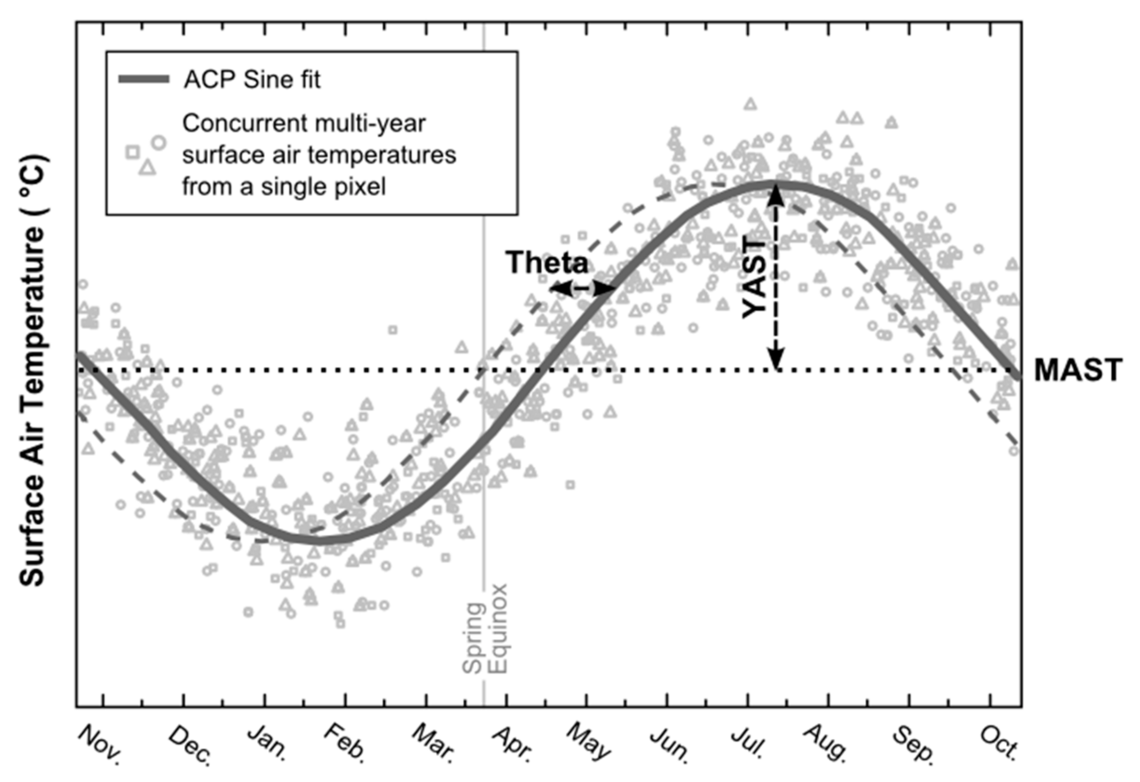
2.2. Heating and Cooling Degree Calculations

PLANHEAT’s HD and CD dataset has been designed to reflect the current average conditions of each city’s UHI at a spatial and temporal resolution of 1 km and 1 h, respectively. For this reason, the HD and CD are calculated from a multiyear dataset of recent (after mid-2016) IAASARS/NOA surface air temperatures that has been aggregated to a synthetic one-year time series of average-like hourly values. The overall workflow for producing PLANHEAT’s HD and CD dataset is presented in Figure 1 and consists of three key processing steps. The first step is to aggregate the IAASARS/NOA multiyear dataset to a set of parameters that describe the average-like diurnal and annual surface air temperature cycle of each pixel; the second step is to use these cycle parameters to generate a synthetic one-year time series of hourly surface air temperatures; and the third and final step is to calculate the hourly HD and CD from the synthetic average-like data.

For midlatitude regions, like Europe, the annual cycle of the surface air temperature can be approximated by a sinusoid function [33]. This work takes advantage of this property and aggregates the multiyear IAASARS/NOA dataset to 24 sets of annual cycle parameters (ACPs)—one set for each hour of the day. The ACPs provide a generalized characterization of the temperature’s temporal dynamics and a gap-free representation of the surface’s thermal characteristics [24,34,35] and are: the mean annual surface temperature (MAST, in °C), the yearly amplitude of surface temperature (YAST, set by definition to be ≥ 0 °C), and the phase shift relative to the spring equinox (theta, set by definition to range between −182.5 and +182.5 d). These three parameters are retrieved by modelling the annual temperature cycle of each pixel using a harmonic (sine) function that is then reduced to the MAST, YAST, and theta parameters, as shown in Figure 2 [35,36]. To retrieve the ACPs for this work, the multiyear IAASARS/NOA dataset is first divided in 24 subsets (one subset for each hour of the day), and then the multiyear data of each subset are stacked according to the day of year (DOY = [1, 2, …, 365]). The sine fitting is then performed for each subset separately, using a least-squares optimization on a pixel-by-pixel basis, and results in 24 sets of corresponding MAST, YAST, and theta raster layers.

The next processing step is to use the aforementioned 24 ACP sets and generate a synthetic one-year time series of hourly surface air temperatures. This is done using Equation (1) for each 1 × 1 km pixel. In this equation, ${\widehat{T}}_{\mathrm{air}}$ is the synthetic surface air temperature (in °C) at datetime d (in decimal DOYs) and ${\mathrm{MAST}}_t$ (in °C), and ${\mathrm{YAST}}_t$ (in °C) and ${\mathrm{Theta}}_t$ (in radians) are the ACPs for the corresponding hour of day t, where t = [1, 2 , …, 24].

$${\widehat{T}}_{\mathrm{air}}\left(d\right)={\mathrm{MAST}}_t+{\mathrm{YAST}}_t\sin \left(\frac{2\pi }{365}d+{\mathrm{Theta}}_t\right).$$

(1)

This step results in a data cube of synthetic surface air temperatures that represent the current average conditions. This data cube includes 8760 values (365 d × 24 h/d) for each 1 × 1 km pixel and is used for calculating PLANHEAT’s hourly HD and CD using Equations (2) and (3), respectively.

$$\mathrm{HD}\left(d\right)=\left\{\begin{array}{cc}{T}_{\mathrm{b},\mathrm{heating}}-{\widehat{T}}_{\mathrm{air}}\left(d\right)& \mathrm{if}{T}_{\mathrm{b},\mathrm{heating}}-{\widehat{T}}_{\mathrm{air}}\left(d\right)\ge 0\\ 0& \mathrm{if}{T}_{\mathrm{b},\mathrm{heating}}-{\widehat{T}}_{\mathrm{air}}\left(d\right)<0\end{array}\right.;$$

(2)

$$\mathrm{CD}\left(d\right)=\left\{\begin{array}{cc}{\widehat{T}}_{\mathrm{air}}\left(d\right)-T_{\mathrm{b},\mathrm{cooling}}& \mathrm{if}{\widehat{T}}_{\mathrm{air}}\left(d\right)-T_{\mathrm{b},\mathrm{cooling}}\ge 0\\ 0& \mathrm{if}{\widehat{T}}_{\mathrm{air}}\left(d\right)-T_{\mathrm{b},\mathrm{cooling}}<0\end{array}\right..$$

(3)

In particular, using Equation (2), the HD data are retrieved as the positive deviation from ${\widehat{T}}_{\mathrm{air}}$ of a base temperature below which it is assumed that heating is needed ($T_{\mathrm{b},\mathrm{heating}}$, in °C). In a similar manner, using Equation (3), the CDs are retrieved as the positive deviation of ${\widehat{T}}_{\mathrm{air}}$ from a base temperature above which it is assumed that cooling is needed ($T_{\mathrm{b},\mathrm{cooling}}$, in °C). The choice of the $T_{\mathrm{b},\mathrm{heating}}$ and $T_{\mathrm{b},\mathrm{cooling}}$ is not straightforward and depends on the local climate, the characteristics of the building stock, and also the thermostat setting of each building [15,37,38]. Because PLANHEAT’s HD and CD dataset covers various cities all over Europe, it is not possible to choose a set of $T_{\mathrm{b},\mathrm{heating}}$ and $T_{\mathrm{b},\mathrm{cooling}}$ that performs optimally for each pixel [15]. For this reason, the PLANHEAT tool, and in particular the PLANHEAT’s district mapping module (DMM) [5], which simulates the hourly thermal energy demand of each building using these hourly HD and CD data as input, uses base temperatures at 15.5 °C for the HD and 22.0 °C for CD as default, but it allows the users to arbitrarily set the optimal $T_{\mathrm{b},\mathrm{heating}}$ and $T_{\mathrm{b},\mathrm{cooling}}$ for their work (as done in [5]). The aforementioned values have been selected because they are used by the European Environmental Agency (EEA) and the Statistical Office of the European Union (Eurostat), and they have also been used for studying the climatology and the trends of HD and CD over Europe for 1951–2010 [15].

In addition to the hourly HD and CD dataset, the PLANHEAT tool also includes an aggregated raster dataset that presents (i) the annual sum of the HD and CD (${\mathrm{HD}}_{\mathrm{Annual}}$ and ${\mathrm{CD}}_{\mathrm{Annual}}$, respectively); and (ii) the annual sum of hours (${\mathrm{HDH}}_{\mathrm{Annual}}$ and ${\mathrm{CDH}}_{\mathrm{Annual}}$, respectively) for which the ${\widehat{T}}_{\mathrm{air}}$ is lower (for HD) and higher (for CD) than the corresponding base temperatures. The former are derived using Equations (4) and (5), respectively, while the latter are derived using Equations (6) and (7), respectively. This aggregated raster dataset has a spatial resolution of 1 × 1 km and has been calculated using, as base temperatures, 15.5 °C and 18.0 °C for HD and 22.0 °C for CD.

$${\mathrm{HD}}_{\mathrm{Annual}}={\sum }_{d=1}^{8760}\mathrm{HD}\left(d\right);$$

(4)

$${\mathrm{CD}}_{\mathrm{Annual}}={\sum }_{d=1}^{8760}\mathrm{CD}\left(d\right);$$

(5)

$${\mathrm{HDH}}_{\mathrm{Annual}}={\sum }_{d=1}^{8760}\mathrm{HDH}\left(d\right)\mathrm{where}\mathrm{HDH}\left(d\right)=\left\{\begin{array}{cc}1& \mathrm{if}{T}_{\mathrm{b},\mathrm{heating}}-{\widehat{T}}_{\mathrm{air}}\left(d\right)\ge 0\\ 0& \mathrm{if}{T}_{\mathrm{b},\mathrm{heating}}-{\widehat{T}}_{\mathrm{air}}\left(d\right)<0\end{array}\right.;$$

(6)

$${\mathrm{CDH}}_{\mathrm{Annual}}={\sum }_{d=1}^{8760}\mathrm{CDH}\left(d\right)\mathrm{where}\mathrm{CDH}\left(d\right)=\left\{\begin{array}{cc}1& \mathrm{if}{\widehat{T}}_{\mathrm{air}}\left(d\right)-T_{\mathrm{b},\mathrm{cooling}}\ge 0\\ 0& \mathrm{if}{\widehat{T}}_{\mathrm{air}}\left(d\right)-T_{\mathrm{b},\mathrm{cooling}}<0\end{array}\right..$$

(7)

3. Results for Antwerp

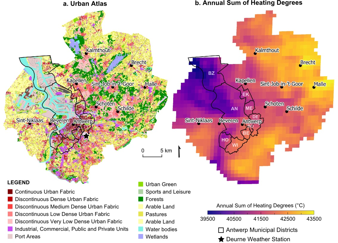
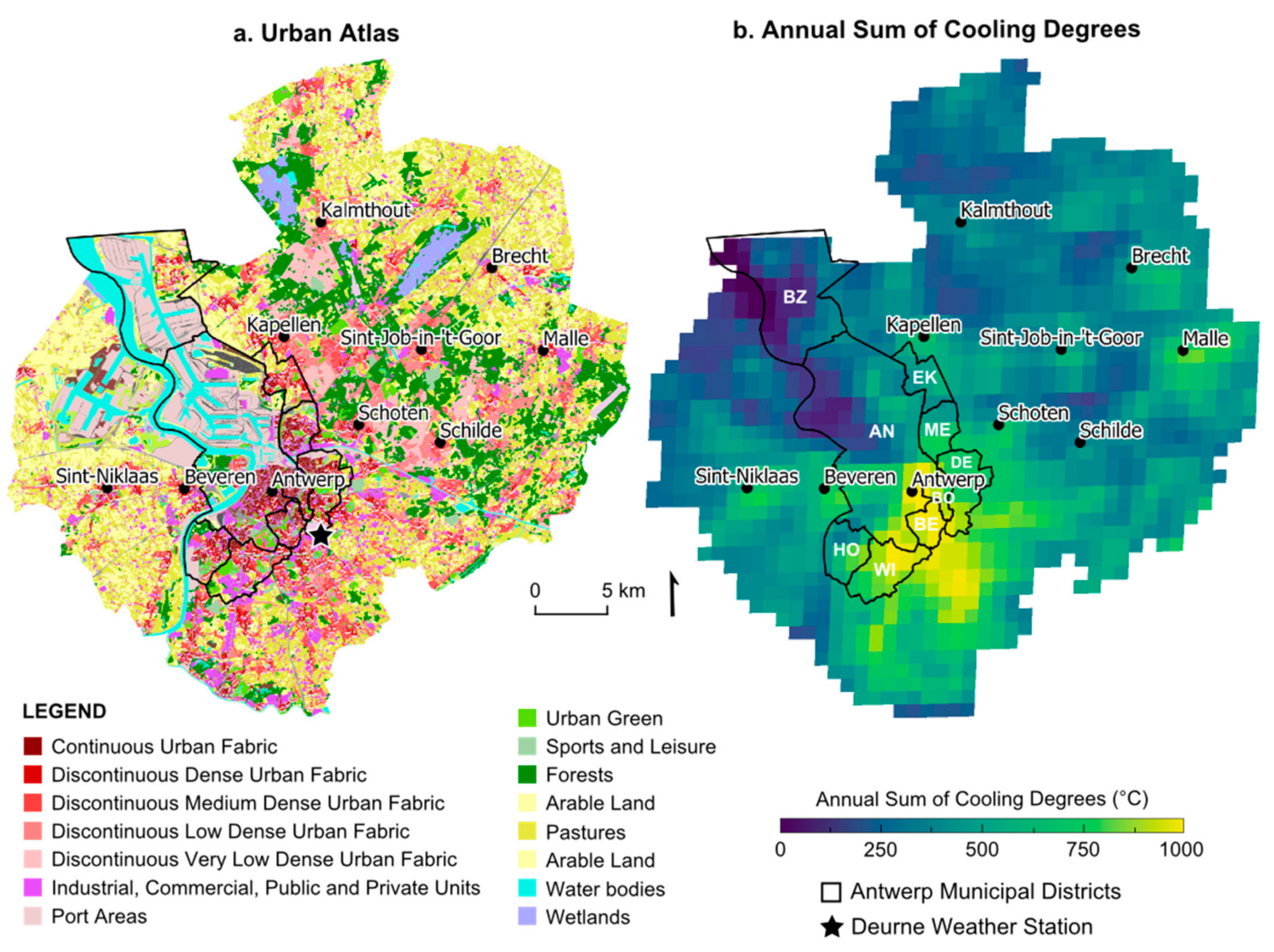
3.1. Antwerp’s Functional Urban Area

Antwerp is a major port city in Belgium and one of the three validation cities of PLANHEAT. It is the capital of the Antwerp Province in the community of Flanders and on 1 January 2018 had a population of 523,245 people. Its metropolitan area accommodates approximately 1,200,000 people, which is surpassed in Belgium only by Brussels. Antwerp’s functional urban area (FUA) covers an area of 1187.03 km², and according to the 2012 European Urban Atlas (UA) dataset [39] the most dominant land cover and land use (LCLU) classes are pastures (21.5%), arable land (15.6%), discontinuous urban fabric (14.4%), forests (11.8%), industrial and commercial units (6.5%), water (5.7%), port areas (5.2%), urban green (2.1%), and continuous urban fabric (2.0%). The Municipality of Antwerp covers an area of 204.51 km² and is located on the River Scheldt, which discharges into the North Sea via the Westerschelde estuary. Antwerp is divided into nine municipal districts, and its port area is one of the 20 largest ports in the world, ranking third in Europe. According to the Köppen climate classification, Antwerp’s climate is oceanic (Köppen: Cfb) with cool summers and cool, but not cold, winters and with a relatively narrow annual temperature range. The mean annual surface air temperature is 10.6 °C, and the warmest and coldest months are July (18.5 °C) and January (3.4 °C), respectively (

Table 1. Climate data for Antwerp, Belgium (1981–2010 normals).

Climate Data	Jan.	Feb.	Mar.	Apr.	May	Jun.	Jul.	Aug.	Sep.	Oct.	Nov.	Dec.	Year
Daily Mean °C	3.4	3.7	6.8	9.6	13.6	16.2	18.5	18.2	15.1	11.3	7.0	4.0	10.6
Average Low °C	0.7	0.5	2.8	4.8	8.8	11.7	13.8	13.2	10.6	7.4	4.1	1.5	6.7
Average High °C	6.2	7.0	10.8	14.4	18.4	20.9	23.2	23.1	19.7	15.3	10.1	6.6	14.7
Mean Precipitation (mm)	69.3	57.4	63.8	47.1	61.5	77.0	80.6	77.3	77.2	78.7	79.0	79.5	848.4

Source: Royal Meteorological Institute of Belgium.

).

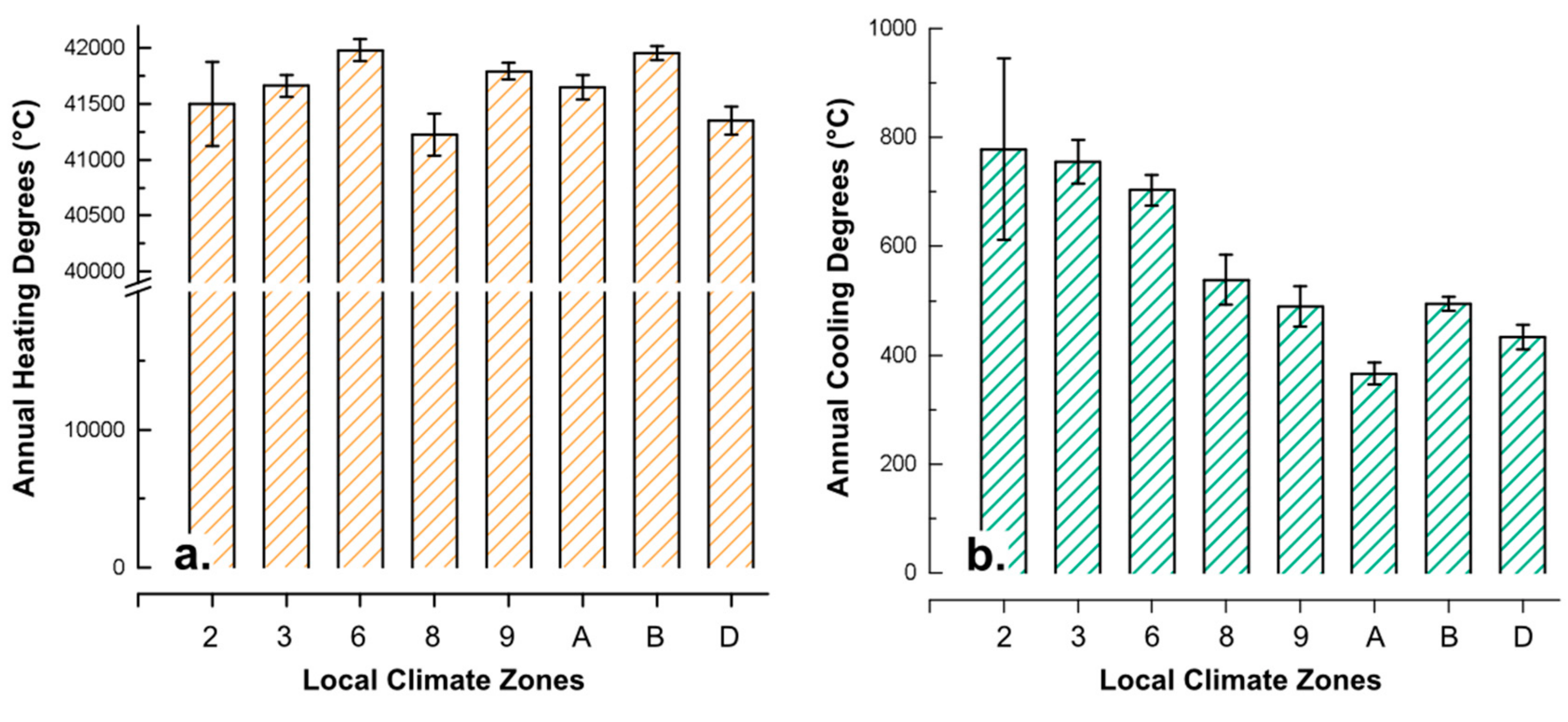
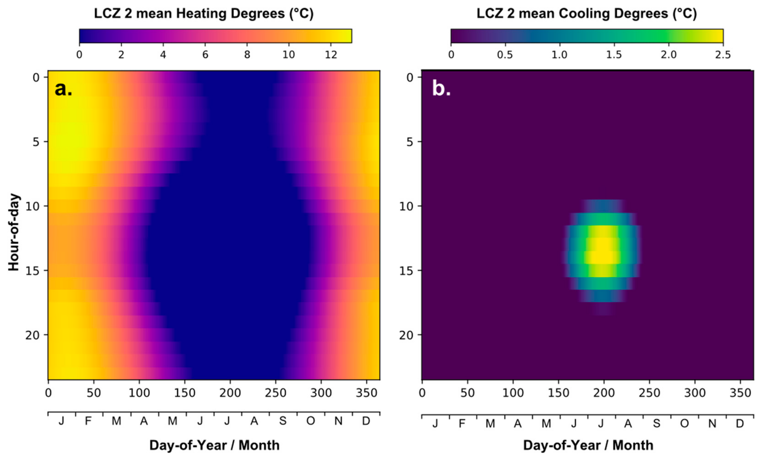
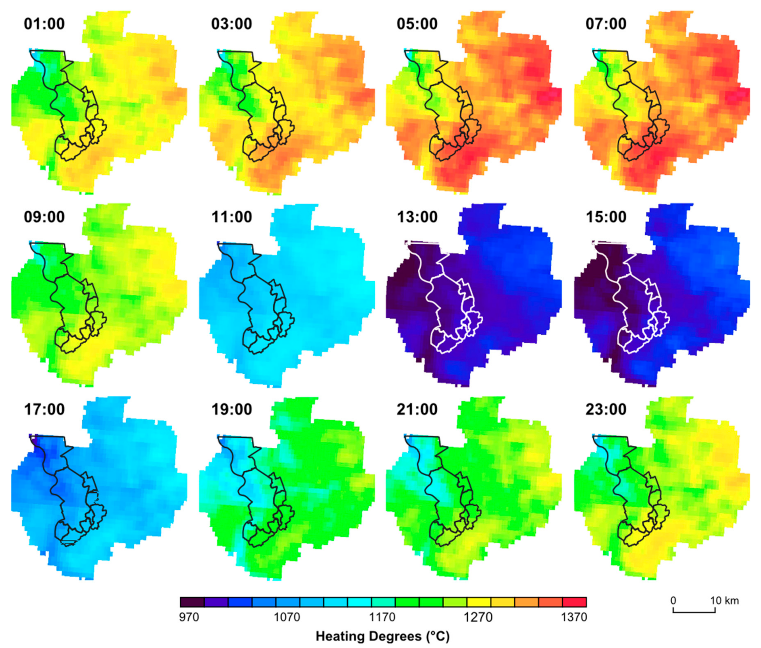
3.2. PLANHEAT’s Heating Degree (HD) and Cooling Degree (CD) Data for Antwerp

Figure 3 and Figure 4 present PLANHEAT’s ${\mathrm{HD}}_{\mathrm{Annual}}$ (for a base temperature of 15.5 °C) and ${\mathrm{CD}}_{\mathrm{Annual}}$ data for Antwerp’s FUA, respectively. The minimum, mean, median, and maximum ${\mathrm{HD}}_{\mathrm{Annual}}$ values are 38,563 °C, 41,818 °C, 41,937 °C, and 43,491°C, respectively. The distribution of the ${\mathrm{HD}}_{\mathrm{Annual}}$ data is negatively skewed (the skewness is −0.6.) and slightly platykurtic with a kurtosis of 2.9. The highest ${\mathrm{HD}}_{\mathrm{Annual}}$ values are found in the east part of Antwerp’s FUA (Figure 3b), where the dominant LCLU classes are pastures and arable land (Figure 3a). In contrast, the lowest ${\mathrm{HD}}_{\mathrm{Annual}}$ values are observed over Antwerp because of the UHI effect and, in particular, over the districts of Antwerp (AN), Borgerhout (BO), Berendrecht-Zandvliet-Lillo (BZ), Ekeren (EK), and Merksem (ME), which include Antwerp’s densely built historic city center and also the port area. The districts of Berchem (BE), Hoboken (HO), Wilrijk (WI), and Deurne (DE), which are closer to the outskirts of the city, have higher ${\mathrm{HD}}_{\mathrm{Annual}}$ values and implies that the need for heating is stronger in AN, BO, BZ, EK, and ME. Figure 3b also shows that water bodies, such as the Scheldt River, influence the HD and result in lower HD values. This can be attributed to the higher heat capacity and thermal inertia of water and also to industrial activities that discharge warm water in the river.

The minimum, mean, medium, and maximum of the ${\mathrm{CD}}_{\mathrm{Annual}}$ presented in Figure 4b are 0 °C, 496 °C, 478 °C, and 1025 °C, respectively. The skewness and kurtosis of the ${\mathrm{CD}}_{\mathrm{Annual}}$ distribution are 0.27 and 3.2, respectively. The highest ${\mathrm{CD}}_{\mathrm{Annual}}$ values are found over Antwerp’s historic city center and also over the WI and BE districts, where the dominant 2012 UA LCLU classes are continuous and discontinuous medium and dense urban fabric. Satellite towns, such as Sint-Niklaas, Brecht, and Malle, also have high CD values with respect to their surroundings and are presented as CD hotspots in Figure 4b. The lowest ${\mathrm{CD}}_{\mathrm{Annual}}$ values correspond to forested areas and areas with water, such as the wetlands east of Kalmthout and Brecht, and also the Scheldt River.

The mean ${\mathrm{HD}}_{\mathrm{Annual}}$ and ${\mathrm{CD}}_{\mathrm{Annual}}$ values for the dominant local climate zones (LCZs) of Antwerp’s FUA are presented in Figure 5 (the LCZ data used here are the World Urban Database and Access Portal Tools, WUDAPT, level-0 data [40,41] for Antwerp, aggregated to PLANHEAT’s 1 × 1 km grid using a majority filter). The LCZ is a standardized, comprehensive, climate-based classification of urban and rural sites for temperature studies [42]. Antwerp’s FUA includes LCZs 2, 3, 6, 8, 9, 10, A, B, and D [43]. The first two correspond to compact mid- and low-rise urban areas with tightly packed buildings and little or no green spaces. LCZs 6 and 9 correspond to areas with sparsely arranged buildings and an abundance of trees and pervious cover, whereas LCZs 8 and 10 correspond to areas with large structures (e.g., for industrial use) with few or no trees and mostly paved surfaces. Lastly, LCZs A, B, and D correspond to forested and low plant areas. Figure 5a shows that in the residential areas (i.e., LCZs 2, 3, 6, and 9) the ${\mathrm{HD}}_{\mathrm{Annual}}$ increases as the urban fabric becomes less dense with lower buildings and the vegetation more abundant. In addition, in the port area, which corresponds to industrial and large low-rise LCZs, the ${\mathrm{HD}}_{\mathrm{Annual}}$ are the lowest, while in the vegetated rural and forested areas (i.e., LCZs A and B) they are the highest. The mean ${\mathrm{CD}}_{\mathrm{Annual}}$ values present the opposite picture, as it can be seen in Figure 5b. Specifically, the residential LCZs that need the most cooling are LCZs 2 and 3, which are tightly packed with mid- and low-rise buildings, and the ones that require the least cooling are LCZs 6 and 9 that have plenty of vegetation and sparsely arranged buildings. In addition, the LCZs with the lowest mean ${\mathrm{CD}}_{\mathrm{Annual}}$ values are the natural classes A, B, and D.

Figure 6 demonstrates the temporal information of PLANHEAT’s HD and CD dataset. In particular, it shows the temporal distribution of the hourly mean HD and CD for Antwerp’s LCZ 2 (10 pixels in total) for an entire year. According to this figure, the coldest months with the most HDs are December, January, and February, while the hottest one with the most CD is July (both observations agree with the climate data of Table 1). The total number of hours for which the hourly mean HDs for LCZ 2 are above 0.5 °C is equal to 5771, which is equivalent to ~65% of the year. In addition, the total number of hours for which the hourly mean CDs are above 0.5 °C is 541 (i.e., ~6% of the year). The maximum hourly mean HD value for LCZ 2 is equal to 13 °C and is observed at DOY 25 at 06:00 UTC, while the corresponding maximum mean CD value is equal to 2.5 °C and is observed at DOY 199 at 15:00 UTC. In general, the highest HD values are found at nighttime around 06:00 UTC, and the highest CD values are found at noon around 14:00 UTC. In addition, according to Figure 6, the longest continuous time periods for which heating or cooling is needed are 24 h and 8 h, respectively.

Last but not least, the change of Antwerp’s HD spatial patterns during the course of a day is presented in Figure 7. The HD of this figure refers to the time period between 1 October and 31 March—when the most heating is needed (used in [15])—and are equal to the pixelwise sum of the corresponding 1 × 1 km hourly HD. In agreement with Figure 6, the HD peak is at around 06:00 UTC and is at a minimum around 15:00 UTC. The HD spatial patterns are strongest during the nighttime and the least pronounced during daytime. The rural areas south and east of Antwerp exhibit the highest HD values, especially between 03:00 and 07:00 UTC, while the port area of Antwerp and the areas adjacent to the River Scheldt exhibit the lowest HD values throughout the day. According to Figure 7, at noon (11:00–15:00 UTC) the nine municipal districts of Antwerp exhibit similar HD values and no distinct major spatial features. Antwerp’s HD spatial patterns start to strengthen after 19:00 UTC and peak at around 07:00 UTC. In particular, the HD of the municipal districts of WI, BE, and BO, which are located at the southern side of Antwerp’s municipality (see Figure 3 or Figure 4) increase faster than that of the other municipalities; they peak at a higher value and have higher HD values with respect to the other districts throughout the night. This is attributed to the lower intensity of the UHI effect near the city outskirts. Similarly, the municipal districts of EM, ME, and DE, which are located at the eastern side of the municipality, also have high HD values throughout the night. On the other hand, the district of Antwerp, which is located at the center of the city and includes most of Antwerp’s port area, has the lowest HD values throughout the day. To that end, at nighttime there is a clear difference between the residential and port area HDs, which most probably is due to UHI effects and the presence of water at the port area.

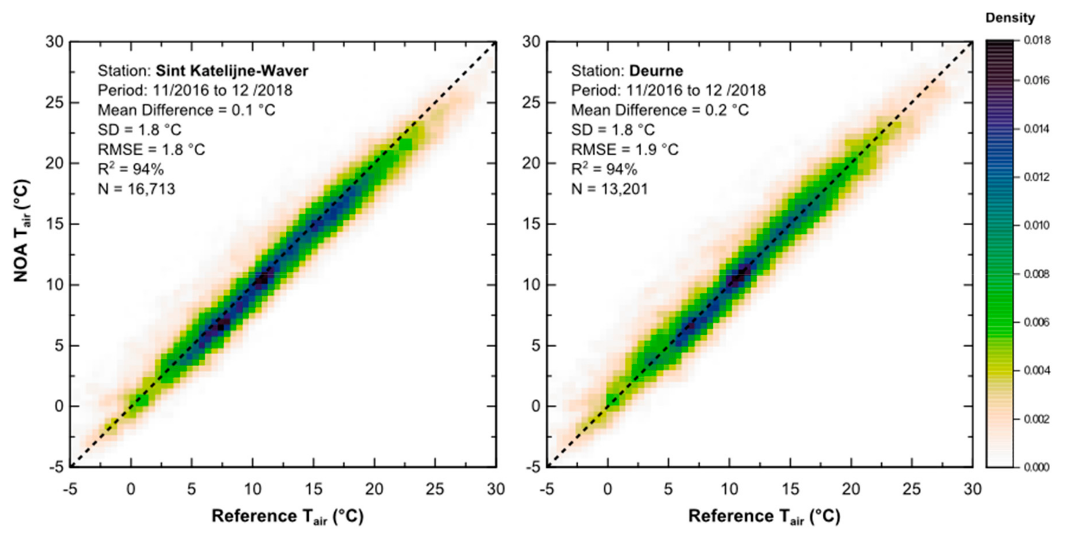
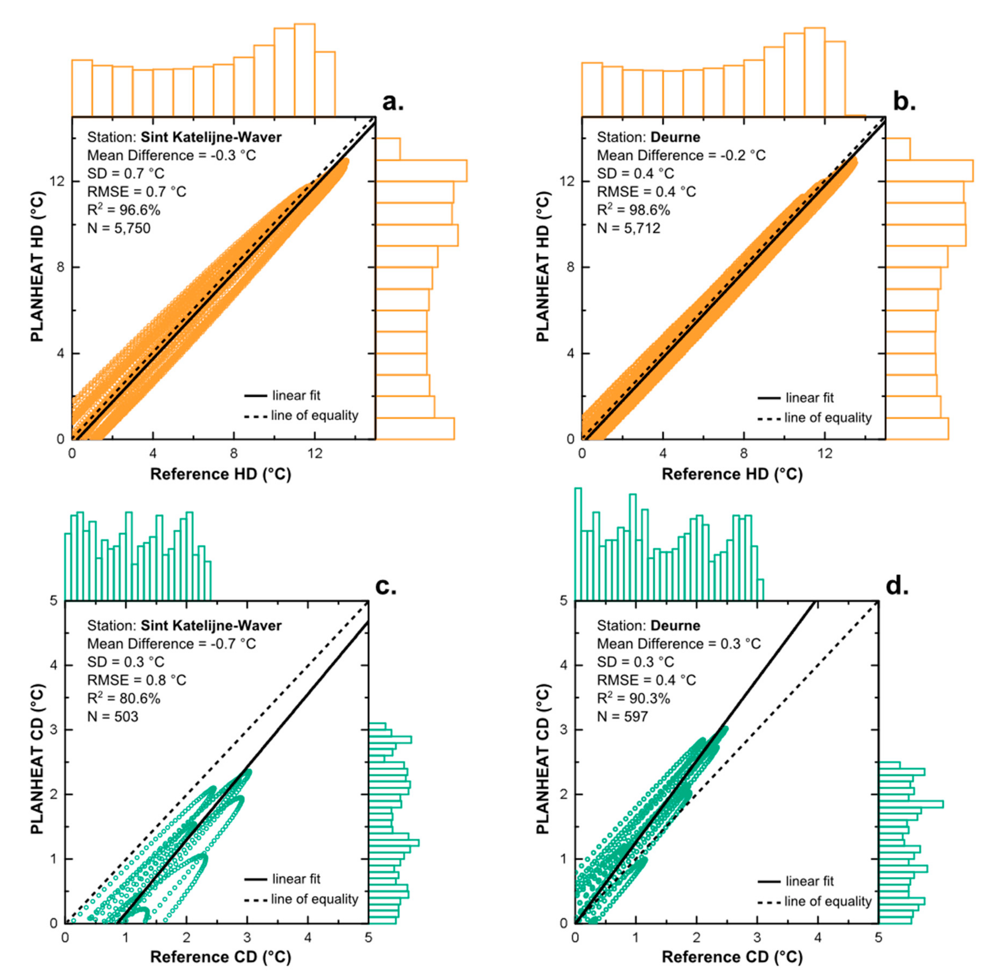
3.3. Accuracy of PLANHEAT’s Hourly HD and CD

The validation of PLANHEAT’s hourly HD and CD is performed in two stages: first, by comparing the original IAASARS/NOA hourly data with concurrent, collocated, in situ surface air temperature measurements, and secondly, by comparing PLANHEAT’s hourly HD and CD with corresponding reference values derived from the aforementioned in situ measurements after applying the ACP-based HD/CD retrieval method of Figure 1. The in situ hourly data cover the time period between 1 November 2016 and 31 December 2018 and are from the Sint Katelijne-Waver (51.083°N, 4.517°E) and Deurne (51.189°N, 4.460°E; star symbol in Figure 3a and Figure 4a) weather stations, which are located close to Antwerp. Specifically, the former is located at a rural site 16 km south of Antwerp, while the latter is 4 km south of the city center at the Antwerp International Airport. The source of the in situ data is NOAA’s National Climatic Data Center (NCDC), which preserves, monitors, assesses, and provides public access to climate and historical weather data and information through the Climate Data Online (CDO) portal.

Figure 8 presents the results of the first validation stage and shows that the IAASARS/NOA surface air temperatures agreed well with the corresponding in situ measurements for both the Sint Katelijne-Waver and the Deurne stations (Figure 8a,b, respectively). In detail, the mean difference was close to 0 °C for both stations, and the standard deviation (SD) was equal to 1.8 °C. The RMSE for Sint Katelijne-Waver was 1.8 °C and was 1.9 °C for Deurne, while the squared correlation coefficient (R²) was equal to 94% for both. The aforementioned statistics have been calculated from 16,713 comparisons for Sint Katelijne-Waver and 13,201 for Deurne.

The results of the second validation stage are presented in Figure 9. In particular, Figure 9a,b present agreement between the PLANHEAT and the in situ hourly HD (base temperature: 15.5 °C) for Sint Katelijne-Waver and Deurne, respectively; while Figure 9c,d present agreement for the corresponding hourly CD (base temperature: 22.0 °C). The validation results suggest that, for Antwerp, the PLANHEAT HD agreed quite well with the reference HD for both stations. Specifically, the mean difference was −0.3 °C for Sint Katelijne-Waver (5750 comparisons) and −0.2 °C for Deurne (5712 comparisons), while the corresponding SDs were 0.7 °C and 0.4 °C, respectively. The RMSE and the R² for Sint Katelijne-Waver were 0.7 °C and 96.6%, respectively, and for Deurne they were 0.4 °C and 98.6%, respectively (Figure 9a,b). Validation of the hourly CD data for Antwerp revealed that the CD mean difference and SD for Sint Katelijne-Waver (503 comparisons) were −0.7 °C and 0.3 °C, respectively, and for Deurne (597 comparisons) +0.3 °C and 0.4 °C, respectively. The corresponding RMSE and R² values were 0.8 °C and 80.6%, and 0.4°C and 90.3%, respectively (Figure 9c,d).

4. Discussion

The results of this work demonstrate the spatial and temporal information of PLANHEAT’s HD and CD dataset, which reflects the current average conditions of each city’s UHI at a spatial and temporal resolution of 1 km and 1 h, respectively. The UHI effects influence the H&C energy demand of buildings, and, if omitted in energy demand simulations, they can result in increased error [12,18,44]. These errors can be so large that Palme et al. [44] challenged the validity of building assessments that do not take the UHI effects into account. Using PLANHEAT’s HD and CD dataset, the users of the PLANHEAT integrated tool can obtain hourly HD and CD data that correspond to their study area and, thus, capture the intensity of the UHI effect at this exact location. This can be a superior alternative to standard meteorological data from airport weather stations that are widely used today but seem to be rather inaccurate to run energy simulations [12,18]. Moreover, users of this dataset can also exploit the extensive spatial coverage of HD and CD data and investigate the spatial patterns of the UHI impacts on the H&C energy consumption of buildings.

In contrast to previous remote sensing works [17,19,20] that retrieve the HDD and CDD from thermal images acquired by sun-synchronous near-polar orbiting satellites (e.g., AVHRR and Landsat), this work utilizes data from Meteosat-10 SEVIRI, which is a geostationary satellite instrument. This is because only geostationary satellite instruments can provide data that capture the diurnal temperature cycle at hourly intervals [22], albeit with a very coarse spatial resolution. To address this issue, the IAASARS/NOA nowcasting service downscales the SEVIRI coarse-scale data to a spatial resolution of 1 km, for which the basic features of UHIs (i.e., the intensity, the spatial extent, the orientation, and the centroid) can be calculated [45,46] (spatiotemporal fusion can also be used to address this issue if corresponding pairs of high- and coarse-resolution surface air temperatures are available [47,48]). Another improvement with respect to previous works is the method used for retrieving the required surface air temperatures. In particular, in [17] and [19] these temperature data are retrieved using a regression model derived from collocated and concurrent satellite-derived LST and in situ surface air temperatures. The applicability of this method depends on the availability and distribution of weather stations, which can become a limiting factor for regions with few weather stations. In addition, the performance of the derived regression models will only be good at the locations and the datetimes for which these models were developed [21]. In contrast to this approach, the data assimilation method used in the IAASARS/NOA nowcasting service [21,29] can be generally applied to any SEVIRI pixel and does not require in situ data.

Overall, satellite thermal image data describe the spatial heterogeneity of the urban thermal environment in much greater detail than spatially interpolated weather station measurements [7]. Hence, satellite data can provide the basis for a more physically realistic HD and CD data product. Typically, computer simulations of buildings and solar energy systems [49,50] use test reference years (TRYs) and typical meteorological years (TMYs), which represent a year of hourly weather data values. TRYs and TMYs are extracted from long-term data records (a minimum of 10 years), do not provide information on extreme events, and do not necessarily represent actual conditions at any given time. However, because the IAASARS/NOA archive of surface air temperatures covers only the last few years, it is not possible to extract TRYs or TMYs for each 1 × 1 km pixel. As a partial workaround to this problem, the input multiyear IAASARS/NOA surface air temperatures are aggregated to a synthetic one-year time series of average-like hourly values using the ACPs. This way it is possible to remove the extreme values from the input surface air temperatures and produce an HD and CD dataset that reflects the current average conditions.

PLANHEAT’s HD and CD dataset is an example of solution-oriented research that provides place-based results with practical utility. This, according to Zhu et al. [51], is an important precondition for practitioners to use urban science and urban remote sensing. To that end, PLANHEAT’s HD and CD have already been used in [5] so as to calculate the current hourly thermal energy demand of each building in Antwerp’s historic city center.

5. Conclusions

UHIs can have significant impacts on the H&C energy consumption of buildings by increasing the cooling energy demand in summer and decreasing the heating energy demand in winter. The PLANHEAT integrated tool includes a dataset of 1 × 1 km, hourly HD and CD that covers several EU cities and reflects the current average conditions of each city’s UHI. This article describes the method for producing this dataset from satellite-derived surface air temperatures and presents its accuracy for the city of Antwerp in Belgium. PLANHEAT’s HD and CD are a key part of PLANHEAT’s city and district mapping modules that map and quantify the current H&C energy demand at city and district levels, respectively. This integrated GIS software tool aims to support municipal and public bodies in the definition, simulation, and evaluation of sustainable H&C strategies and is freely available as a QGIS3 plugin.

References

1. European Commission. A Clean Planet for All. A European Strategic Long-Term Vision for a Prosperous, Modern, Competitive and Climate Neutral Economy; European Commission: Brussels, Belgium, 2018. [Google Scholar]
2. European Commission. An EU Strategy on Heating and Cooling; European Commission: Brussels, Belgium, 2016. [Google Scholar]
3. Pablo-Romero, M.d.P.; Sánchez-Braza, A.; González-Limón, J.M. Covenant of Mayors: Reasons for Being an Environmentally and Energy Friendly Municipality. Rev. Policy Res. 2015, 32, 576–599. [Google Scholar] [CrossRef]
4. QGIS Development Team. QGIS Geographic Information System; QGIS Development Team: Beaverton, OR, USA, 2019. [Google Scholar]
5. Oregi, X.; Hermoso, N.; Prieto, I.; Izkara, J.L.; Mabe, L.; Sismanidis, P. Automatised and georeferenced energy assessment of an Antwerp district based on cadastral data. Energy Build. 2018, 173, 176–194. [Google Scholar] [CrossRef]
6. Santamouris, M.; Papanikolaou, N.; Livada, I.; Koronakis, I.; Georgakis, C.; Argiriou, A.; Assimakopoulos, D. On the impact of urban climate on the energy consumption of buildings. Sol. Energy 2001, 70, 201–216. [Google Scholar] [CrossRef]
7. Li, X.; Zhou, Y.; Yu, S.; Jia, G.; Li, H.; Li, W. Urban heat island impacts on building energy consumption: A review of approaches and findings. Energy 2019, 174, 407–419. [Google Scholar] [CrossRef]
8. Santamouris, M. On the energy impact of urban heat island and global warming on buildings. Energy Build. 2014, 82, 100–113. [Google Scholar] [CrossRef]
9. Oke, T.R. The energetic basis of the urban heat island. Q. J. R. Meteorol. Soc. 1982, 108, 1–24. [Google Scholar] [CrossRef]
10. Oke, T.R.; Mills, G.; Christen, A.; Voogt, J.A. Urban Climates; Cambridge University Press: Cambridge, UK, 2017; ISBN 0521849500. [Google Scholar]
11. Zinzi, M.; Carnielo, E. Impact of urban temperatures on energy performance and thermal comfort in residential buildings. The case of Rome, Italy. Energy Build. 2017, 157, 20–29. [Google Scholar] [CrossRef]
12. Salvati, A.; Coch Roura, H.; Cecere, C. Assessing the urban heat island and its energy impact on residential buildings in Mediterranean climate: Barcelona case study. Energy Build. 2017, 146, 38–54. [Google Scholar] [CrossRef] [Green Version]
13. Kolokotroni, M.; Ren, X.; Davies, M.; Mavrogianni, A. London’s urban heat island: Impact on current and future energy consumption in office buildings. Energy Build. 2012, 47, 302–311. [Google Scholar] [CrossRef]
14. European Environment Agency. Heating and Cooling Degree Days; European Environment Agency: Copenhagen, Denmark, 2016. [Google Scholar]
15. Spinoni, J.; Vogt, J.; Barbosa, P. European degree-day climatologies and trends for the period 1951–2011. Int. J. Climatol. 2014, 35, 25–36. [Google Scholar] [CrossRef]
16. Thom, H.C.S. The rational relationship between heating degree days and temperature. Mon. Weather Rev. 1954, 82, 1–6. [Google Scholar] [CrossRef]
17. Stathopoulou, M.; Cartalis, C.; Chrysoulakis, N. Using midday surface temperature to estimate cooling degree-days from NOAA-AVHRR thermal infrared data: An application for Athens, Greece. Sol. Energy 2006, 80, 414–422. [Google Scholar] [CrossRef]
18. Radhi, H.; Sharples, S. Quantifying the domestic electricity consumption for air-conditioning due to urban heat islands in hot arid regions. Appl. Energy 2013, 112, 371–380. [Google Scholar] [CrossRef]
19. Mushore, T.D.; Odindi, J.; Dube, T.; Mutanga, O. Understanding the relationship between urban outdoor temperatures and indoor air-conditioning energy demand in Zimbabwe. Sustain. Cities Soc. 2017, 34, 97–108. [Google Scholar] [CrossRef]
20. Rahimikhoob, A.; Behbahani, S.; Nazarifar, M.H. Estimation of cooling degree days (CDDs) from AVHRR data and an MLF neural network. Can. J. Remote Sens. 2008, 34, 596–600. [Google Scholar] [CrossRef]
21. Keramitsoglou, I.; Kiranoudis, C.; Sismanidis, P.; Zakšek, K. An Online System for Nowcasting Satellite Derived Temperatures for Urban Areas. Remote Sens. 2016, 8, 306. [Google Scholar] [CrossRef]
22. Sismanidis, P.; Keramitsoglou, I.; Kiranoudis, C.T. A satellite-based system for continuous monitoring of Surface Urban Heat Islands. Urban Clim. 2015, 14, 141–153. [Google Scholar] [CrossRef]
23. Schmetz, J.; Pili, P.; Tjemkes, S.; Just, D.; Kerkmann, J.; Rota, S.; Ratier, A. An introduction to Meteosat Second Generation (MSG). Bull. Am. Meteorol. Soc. 2002, 83, 977–992. [Google Scholar] [CrossRef]
24. Sismanidis, P.; Bechtel, B.; Keramitsoglou, I.; Kiranoudis, C.T. Mapping the Spatiotemporal Dynamics of Europe’s Land Surface Temperatures. IEEE Geosci. Remote Sens. Lett. 2018, 15, 202–206. [Google Scholar] [CrossRef]
25. Global Climate and Weather Modeling Branch. The GFS Atmospheric Model—NCEP Office Note 442; Global Climate and Weather Modeling Branch: Camp Springs, MD, USA, 2003. [Google Scholar]
26. Fernandez, P. Software User Manual for the SAFNWC/MSG Application: Software Part (SAF/NWC/CDOP/INM/SW/SUM/2); EUMETSAT NWCSAF: Madrid, Spain, 2012. [Google Scholar]
27. Derrien, M.; Gleau, H.L.; Fernandez, P. Algorithm Theoretical Basis Document for “Cloud Products” (CMa-PGE01 v3.2, CT-PGE02 v2.2 & CTTH-PGE03 v2.2); NWC SAF: Madrid, Spain, 2013. [Google Scholar]
28. Derrien, M.; Gleau, H.L.; Fernandez, P. Validation Report for “Cloud Products” (CMa-PGE01 v3.2, CT-PGE02 v2.2 & CTTH-PGE03 v2.2); NWC SAF: Madrid, Spain, 2013. [Google Scholar]
29. Martinez, M.A.; Manso, M.; Fernández, P. Algorithm Theoretical Basis Document for “SEVIRI Physical Retrieval” (SPhR-PGE13 v2.0); NWC SAF: Madrid, Spain, 2013. [Google Scholar]
30. Keramitsoglou, I.; Kiranoudis, C.T.; Weng, Q. Downscaling Geostationary Land Surface Temperature Imagery for Urban Analysis. IEEE Geosci. Remote Sens. Lett. 2013, 10, 1253–1257. [Google Scholar] [CrossRef]
31. Sismanidis, P.; Keramitsoglou, I.; Kiranoudis, C.T.; Bechtel, B. Assessing the Capability of a Downscaled Urban Land Surface Temperature Time Series to Reproduce the Spatiotemporal Features of the Original Data. Remote Sens. 2016, 8, 274. [Google Scholar] [CrossRef]
32. Sismanidis, P.; Keramitsoglou, I.; Bechtel, B.; Kiranoudis, C.T. Improving the downscaling of diurnal land surface temperatures using the annual cycle parameters as disaggregation kernels. Remote Sens. 2017, 9, 23. [Google Scholar] [CrossRef]
33. Mckinnon, K.A.; Stine, A.R.; Huybers, P. The spatial structure of the annual cycle in surface temperature: Amplitude, phase, and lagrangian history. J. Clim. 2013, 26, 7852–7862. [Google Scholar] [CrossRef]
34. Bechtel, B. Robustness of Annual Cycle Parameters to Characterize the Urban Thermal Landscapes. IEEE Geosci. Remote Sens. Lett. 2012, 9, 876–880. [Google Scholar] [CrossRef]
35. Bechtel, B. A New Global Climatology of Annual Land Surface Temperature. Remote Sens. 2015, 7, 2850–2870. [Google Scholar] [CrossRef] [Green Version]
36. Bechtel, B.; Sismanidis, P. Time Series Analysis of Moderate Resolution Land Surface Temperatures. In Remote Sensing Time Series Image Processing; Weng, Q., Ed.; CRC Press: Boca Raton, FL, USA, 2018; pp. 89–120. ISBN 9781138054592. [Google Scholar]
37. Büyükalaca, O.; Bulut, H.; Yılmaz, T. Analysis of variable-base heating and cooling degree-days for turkey. Appl. Energy 2001, 69, 269–283. [Google Scholar] [CrossRef]
38. Papakostas, K.; Kyriakis, N. Heating and cooling degree-hours for Athens and Thessaloniki, Greece. Renew. Energy 2005, 30, 1873–1880. [Google Scholar] [CrossRef]
39. Montero, E.; Van Wolvelaer, J.; Garzón, A. The European Urban Atlas. In Land Use and Land Cover Mapping in Europe; Manakos, I., Braun, M., Eds.; Springer: Dordrecht, The Netherlands, 2014; pp. 115–124. [Google Scholar]
40. Bechtel, B.; Alexander, P.J.; Beck, C.; Brousse, O.; Ching, J.; Demuzere, M.; Gal, T.; Hidalgo, J.; Hoffman, P.; Middel, A.; et al. Generating WUDAPT Level 0 data–current status of production and evaluation. Urban Clim. 2019, 27, 24–45. [Google Scholar] [CrossRef]
41. Ching, J.; Mills, G.; Bechtel, B.; See, L.; Feddema, J.; Wang, X.; Ren, C.; Brousse, O.; Martilli, A.; Neophytou, M.; et al. World Urban Database and Access Portal Tools (WUDAPT), an urban weather, climate and environmental modeling infrastructure for the Anthropocene. Bull. Am. Meteorol. Soc. 2018, 99, 1907–1924. [Google Scholar] [CrossRef]
42. Stewart, I.D.; Oke, T. Local Climate Zones for Urban Temperature Studies. Bull. Am. Meteorol. Soc. 2012, 93, 1879–1900. [Google Scholar] [CrossRef]
43. Verdonck, M.-L.; Okujeni, A.; van der Linden, S.; Demuzere, M.; De Wulf, R.; Van Coillie, F. Influence of neighbourhood information on ‘Local Climate Zone’ mapping in heterogeneous cities. Int. J. Appl. Earth Obs. Geoinf. 2017, 62, 102–113. [Google Scholar] [CrossRef]
44. Palme, M.; Inostroza, L.; Villacreses, G.; Lobato-Cordero, A.; Carrasco, C. From urban climate to energy consumption. Enhancing building performance simulation by including the urban heat island effect. Energy Build. 2017, 145, 107–120. [Google Scholar] [CrossRef]
45. Zakšek, K.; Oštir, K. Downscaling land surface temperature for urban heat island diurnal cycle analysis. Remote Sens. Environ. 2012, 117, 114–124. [Google Scholar] [CrossRef]
46. Keramitsoglou, I.; Kiranoudis, C.T.; Ceriola, G.; Weng, Q.; Rajasekar, U. Identification and analysis of urban surface temperature patterns in Greater Athens, Greece, using MODIS imagery. Remote Sens. Environ. 2011, 115, 3080–3090. [Google Scholar] [CrossRef]
47. Wu, P.; Shen, H.; Zhang, L.; Göttsche, F.-M. Integrated fusion of multi-scale polar-orbiting and geostationary satellite observations for the mapping of high spatial and temporal resolution land surface temperature. Remote Sens. Environ. 2015, 156, 169–181. [Google Scholar] [CrossRef]
48. Quan, J.; Zhan, W.; Ma, T.; Du, Y.; Guo, Z.; Qin, B. An integrated model for generating hourly Landsat-like land surface temperatures over heterogeneous landscapes. Remote Sens. Environ. 2018, 206, 403–423. [Google Scholar] [CrossRef]
49. Lee, K.; Yoo, H.; Levermore, G.J. Generation of typical weather data using the ISO Test Reference Year (TRY) method for major cities of South Korea. Build. Environ. 2010, 45, 956–963. [Google Scholar] [CrossRef]
50. Levermore, G.J.; Parkinson, J.B. Analyses and algorithms for new test reference years and design summer years for the UK. Build. Serv. Eng. Res. Technol. 2006, 27, 311–325. [Google Scholar] [CrossRef]
51. Zhu, Z.; Zhou, Y.; Seto, K.C.; Stokes, E.C.; Deng, C.; Pickett, S.T.A.; Taubenböck, H. Understanding an urbanizing planet: Strategic directions for remote sensing. Remote Sens. Environ. 2019, 228, 164–182. [Google Scholar] [CrossRef]
Figure 1. The workflow for retrieving the heating degree (HD) and cooling degree (CD) data from a multiyear time-series of hourly surface air temperatures.
Remotesensing 11 02048 g001
Figure 2. The annual cycle parameter (ACP) retrieval principle.
Remotesensing 11 02048 g002
Figure 3. (a) The 2012 Urban Atlas land cover and land use (LCLU) for Antwerp’s functional urban area (FUA) and (b) the PLANHEAT aggregated (annual sum) HD calculated using a base temperature of 15.5 °C.
Remotesensing 11 02048 g003
Figure 4. (a) The 2012 Urban Atlas LCLU for Antwerp’s FUA and (b) the PLANHEAT aggregated (annual sum) CD calculated using a base temperature of 22.0 °C.
Remotesensing 11 02048 g004
Figure 5. The mean (a) HD Annual (base temperature: 15.5 °C) and (b) CD Annual values (with the corresponding 95% confidence intervals) for the dominant local climate zone (LCZ) of Antwerp’s FUA. LCZ 2: compact midrise; LCZ 3: compact low-rise; LCZ 6: open low-rise; LCZ 8: large low-rise; LCZ 9: sparsely built; LCZ A: dense trees; LCZ B: scattered trees; and LCZ D: low plants.
Remotesensing 11 02048 g005
Figure 6. The hourly mean (a) HD (base temperature: 15.5 °C) and (b) CD for Antwerp’s LCZ 2.
Remotesensing 11 02048 g006
Figure 7. The hourly sum of HD (base temperature: 15.5 °C) for Antwerp’s FUA for the time period between 1 October and 31 March.
Remotesensing 11 02048 g007
Figure 8. Density plots presenting the IAASARS/NOA vs. in situ surface air temperatures for (a) the Sint Katelijne-Waver weather station and (b) the Deurne weather station.
Remotesensing 11 02048 g008
Figure 9. Scatterplots presenting the PLANHEAT vs. reference HD (base temperature: 15.5 °C) and CD for (a,c) the Sint Katelijne-Waver and (b,d) the Deurne weather stations, respectively.
Remotesensing 11 02048 g009