Supervised Distance-Based Feature Selection for Hyperspectral Target Detection


1
Department of Photogrammetry and Remote Sensing, Faculty of Geodesy and Geomatics Engineering, K.N. Toosi University of Technology, Tehran 19967-15433, Iran
2
GeoInfoSolutions BV, Adastraat 33, 7607 HA Almelo, The Netherlands
3
Department of Geomatics Engineering, School of Civil Engineering, Iran University of Science and Technology, Tehran 16846-13114, Iran
*
Author to whom correspondence should be addressed.
Remote Sens. 2019, 11(17), 2049; https://0-doi-org.brum.beds.ac.uk/10.3390/rs11172049
Submission received: 25 July 2019
/
Revised: 18 August 2019
/
Accepted: 24 August 2019
/
Published: 30 August 2019
(This article belongs to the Section Remote Sensing Image Processing)
Abstract
:Feature/band selection (FS/BS) for target detection (TD) attempts to select features/bands that increase the discrimination between the target and the image background. Moreover, TD usually suffers from background interference. Therefore, bands that help detectors to effectively suppress the background and magnify the target signal are considered to be more useful. In this regard, three supervised distance-based filter FS methods are proposed in this paper. The first method is based on the TD concept. It uses the image autocorrelation matrix and the target signature in the detection space (DS) for FS. Features that increase the first-norm distance between the target energy and the mean energy of the background in DS are selected as optimal. The other two methods use background modeling via image clustering. The cluster mean spectra, along with the target spectrum, are then transferred into DS. Orthogonal subspace projection distance (OSPD) and first-norm distance (FND) are used as two FS criteria to select optimal features. Two datasets, HyMap RIT and SIM.GA, are used for the experiments. Several measures, i.e., true positives (TPs), false alarms (FAs), target detection accuracy (TDA), total negative score (TNS), and the receiver operating characteristics (ROC) area under the curve (AUC) are employed to evaluate the proposed methods and to investigate the impact of FS on the TD performance. The experimental results show that our proposed FS methods, as compared with five existing FS methods, have improving impacts on common target detectors and help them to yield better results.

1. Introduction
Hyperspectral imagery (HSI) have properties that provide scientists with various applications, such as crop and mineral identification in agriculture and geology, improved classification map production [1], subpixel target and anomaly detection [2,3,4,5,6,7], spectral unmixing [8], and data fusion. However, huge data volumes are produced due to the high number of spectral bands. Moreover, much of the information that is supplied by hyperspectral data is redundant, since adjacent spectral bands are highly correlated. Hence, studies have been conducted on reducing the data dimensionality by feature/band selection (FS/BS) and feature extraction (FE) methods. In general, the goal of dimensionality reduction (DR) is to reduce data volume, speed up computing, and improve the accuracy of analyses [9,10].
FE methods, such as principal components analysis (PCA) [11], maximum noise fraction (MNF) [12], linear discriminant analysis (LDA) [13], independent components analysis (ICA) [14], and wavelet transform [15] produce new features from a linear combination of the original bands. FE methods have received less attention in target detection (TD) studies since subtle information regarding the target and the background may be lost in this approach. However, there is a new type of FE methods that is based on the deep learning concept, such as the convolutional neural network (CNN) and deep belief network (DBN), which are used to extract new high-level features in order to improve the classification accuracy [16,17].
As for FS methods, there are three main categories: filter, wrapper, and embedded methods [18]. Each of these categories is further divided into supervised and unsupervised methods [19]. Supervised methods rely on training samples and prior information of classes, targets, and background to conduct FS, while unsupervised methods use no prior knowledge. The filter methods select features that are independent of the subsequent image analysis to be conducted, such as classification. The selected features are then given as input to the classifier. Several unsupervised filter methods have been developed, based on the information theory, which use criteria, such as correlation coefficient [18], entropy [20], mutual information [21], linear prediction error (LPE) [22], first/second spectral derivative, contrast, and spectral ratio [20]. Some unsupervised FS methods employ search strategies, such as sequential forward/backward selection (SFS/SBS) and sequential floating forward/backward selection (SFFS/SFBS) [23], which are computing-intensive and yield suboptimal results. Other unsupervised criteria, such as fuzzy logic [24], clonal selection [25], Inf-FS [26], and eigenvector centrality (EC) FS [27], have also been used for FS. In contrast, there are supervised filter methods that are based on distance metrics, such as the Euclidean, Mahalanobis, and Bhattacharyya distances [18]. Other supervised FS methods to be mentioned are gain ratio, chi-square feature evaluation, Relief-F, and correlation-based feature selection (CFS) [18].
Furthermore, some unsupervised filter methods have applied the endmember extraction (EE) criteria [28], which select the most distinctive features as optimal. Examples of such methods are G-FS [29], linear prediction (LP) [30], and orthogonal subspace projection (OSP)-based [31] techniques. These three methods are developed based on the N-FINDR [32], unsupervised fully-constrained least squares (UFCLS) [33], and automatic target generation process (ATGP) [31] measures, respectively. In another class of unsupervised filter FS methods, such as PFS and MTD [34], optimal features are selected based on the geometrical properties of features in the prototype space [35].
In contrast to the filter FS methods, there are several supervised wrapper FS methods. These methods select features that are based on the classification results. Therefore, the FS is iteratively completed. The random forest (RF) and support vector machine recursive feature elimination (SVM-RFE) classifiers have been used as wrappers in [18]. The genetic algorithm (GA) has also been used as a supervised FS method [36]. Furthermore, a kernel-based supervised wrapper FS method developed for SVM can be found in [37].
There are embedded FS methods in addition to the filter and wrapper FS methods. The embedded methods are quite similar to the wrapper methods. The difference to the wrapper methods is that an intrinsic model building metric is used during learning. Examples of embedded methods are L1 regularization (LASSO) [38] and decision tree [39].
A fact to be noticed is that the criteria developed in the literature for FS/FE are mostly used for classification. However, classification and detection are conceptually different. To be more specific, the targets are very rare in an image in terms of the number of pixels. Moreover, many targets are smaller than the ground sampling distance (GSD). Hence, practically no spatial and statistical information can be extracted from them. The only available information is the mixed spectra. Furthermore, a challenge is to suppress the background since it deteriorates the accuracy of TD. In this regard, features that help discriminate the targets from the background are considered to be optimal. Therefore, the DR methods employed for classification might not be as helpful for TD.
Several filter FS methods, supervised and unsupervised, which are aimed at improving TD have been introduced in the literature. For example, in an unsupervised manner, features with more skewness or deviations from the Gaussian distribution are considered to be optimal for TD in [40]. In [41], features that produce better edge maps are regarded to be more informative in an unsupervised fashion. PSO-MSR employs a band search strategy that is based on the particle swarm optimization (PSO) along with a supervised target-background separation ratio in [42] in order to improve TD. Some unsupervised FS methods use band clustering and ranking. For instance, in clustering-based band selection (CBS) [43], band clustering is conducted while using the density-based spatial clustering of applications with noise (DBSCAN) [44] algorithm. The clustered bands are then sorted and selected based on divergence.
In another type of supervised FS, methods are based on similarity measures. Variable-number variable-band selection (VNVBS) [45] uses the concept of orthogonal subspace projection (OSP) to select bands that contain the most discriminatory information. Moreover, some supervised FS methods rank and select bands based on weights. In band selection for CEM (BSC) [46], the feature vector values of the constrained energy minimization (CEM) detector [47] are regarded as the weights of bands. CEM-based constrained band selection (CCBS) [48] also exploits the CEM detector to select the bands. In this unsupervised filter method, each band vector is thought of as the desired target vector and all of the remaining band vectors are regarded as undesired. The output of the finite impulse response (FIR) filter is used as the FS criterion. CCBS uses virtual dimensionality (VD) [49] to determine the signal subspace dimension or the number of bands to be selected. Constrained band subset selection (CBSS) [50] is another unsupervised FS method that is similar to CCBS. The difference is that CBSS constrains multiple bands as a subset as opposed to CCBS, which constrains a single band as a singleton set. In the unsupervised band add-on (BAO) method, a decomposition of the spectral angle mapper (SAM) is presented to select optimal bands based on the angular separation [51].
In contrast, there is also wrapper FS methods that are designed for TD. In [52], for a fixed false alarm (FA) value, the power of detection, PD, is used as the criterion to evaluate the selected features in a supervised fashion. Feature subsets are selected while using the SFS search strategy. Curve area and genetic theory (CAGT) [53] uses the genetic algorithm as the search strategy to find the optimal feature subset. The receiver operating characteristics (ROC) [54] area under the curve (AUC) is used as the supervised criterion to evaluate each feature subset.
Furthermore, there are embedded FS methods that are designed for TD. A supervised sparsity-based method, called LASSO-based band selection (LBS), has been developed to select different band subsets that are based on the CEM detector [55]. The band subset that minimizes the objective function is selected as optimal. In [56], CEM feature vectors have been interpreted based on a sparsity model similar to [55] in which bands with non-zero weights are selected. Moreover, recently, a few studies have been dedicated to applying deep learning concept to TD. For example, in [57], a method, called the CNN-based target detection (CNNTD), was employed to extract features for TD.
It must be noticed that an ideal FS method is one that helps target detectors to more effectively discriminate the target and the image background. Therefore, developing an FS method that is based on the TD concept would help to select more discriminative features. In this regard, the first proposed supervised filter method, called autocorrelation-based feature selection (AFS), innovatively utilizes the image autocorrelation matrix as well as the target signature to simultaneously include the target and the background separation or distance information in the FS process. This is in contrast to many unsupervised FS methods, which only rely on the background information, and many supervised methods, which only use the target information and little background information. The other innovative feature of this method is that it introduces the detection space (DS) to select the optimal features. Indeed, the performance of an FS method depends on the efficiency of the FS criterion and the space that is used for data representation. In addition, it would be ideal to characterize the background, so that more useful information regarding the target and the background separability can be extracted. Hence, in the second proposed supervised filter approach, called target-background separability (TBS), at first, background modeling is performed via the K-Means method [58]. Subsequently, the target spectrum and the cluster mean spectra are projected into the detection space. To conduct FS, two methods that are based on two different criteria, i.e., the orthogonal subspace projection distance (OSPD) and the first-norm distance (FND), are proposed. The innovation of these two methods is they model the background prior to FS and avoid using all background pixels, since neighbouring pixels are usually highly correlated. In addition, they use geometrical measures to select optimal the features in the detection space. Therefore, it must be emphasized that AFS, OSPD, and FND have three key characteristics, i.e., (1) they implement statistical and geometrical FS criteria in the detection space, (2) exploit the target and the background information together as opposed to many of the existing FS methods, and (3) measure three types of distances between the target and the background.
Therefore, this paper is organized, as follows. In Section 2, the datasets that were used for experiments are introduced. Subsequently, five existing TD-based FS methods, i.e., CCBS, VNVBS, BAO, LBS, and PSO-MSR, are briefly introduced for comparison. Furthermore, the concepts behind the three proposed FS methods are explained completely, followed by the explanation of the evaluation measures. Section 3 presents the experiments and results. Section 4 provides discussions regarding the performance of the proposed methods. For detection, the CEM and adaptive matched filter (AMF) [59] detectors are employed. Finally, Section 5 gives the conclusion.
2. Data and Methods
2.1. HyMap Dataset
The HyMap dataset was collected in July 2006 in Cooke City, Montana, USA [60]. The GSD of the image is approximately 3 m. The data contains 126 spectral bands in the VNIR-SWIR range. Water absorption and low signal-to-noise bands were removed, leaving 112 bands. Civilian vehicles and small fabric panels are used as targets. The locations of the ground truth objects or targets are shown in the circles in Figure 1. Zoomed views of the target locations can be seen in Figure 2. Table 1 shows the details of the number, size, and type of the targets. Moreover, the HyMap dataset and all of the information regarding the ground truth given in Figure 1, Figure 2, and Table 1 are available online at [61].
It must be added that the ground truth samples consist of pure and mixed pixels, as well as guard pixels that separate the target panels from the surrounding areas. In our experiments, the guard pixels were removed from the targets list. Furthermore, for targets F1 and F2, the spectra of the central pure pixels were given as input to target detectors. F3 and F4 are arranged in two sizes. Therefore, they are considered as F3a, F3b, F4a, and F4b. F3a and F4a have central pure pixels, but F3b and F4b only consist of mixed pixels. As a result, for F3a and F4a, pure pixels and, for F3b and F4b, mixed pixels are used as target spectra. For targets V1, V2, and V3, only mixed pixels were available, which were inevitably used as input to the detectors. Meanwhile, the HyMap dataset is geometrically and radiometrically corrected and the pixel values demonstrate the reflectance spectra. In Figure 3, the reflectance spectra of the targets are shown. As can be seen, most of the targets have spectral responses that are similar to those of the background vegetation. This implies a very difficult condition to separate the targets from the background.
Meanwhile, in this research, the reflectance values of the HyMap dataset pixels are multiplied by 10,000 to avoid floating-point computation complexities.
2.2. SIM.GA Dataset
The SIM.GA dataset was collected in May 2013 in Viareggio, Italy [62]. It contains 511 spectral bands in the VNIR region. There is also a 127-band binned noise-whitened dataset in the blue and green spectral region, which is used in this research for reduced data size and faster computations. The GSD is about 60 cm. The locations of the ground truth target panels are shown in circles in Figure 4. Table 2 demonstrates the names and number of pixels for each target.
For the SIM.GA dataset, no information regarding the purity or mixture of target pixels was available. Hence, for each target, the mean radiance spectrum of the inner pixels was used as input for detection. In addition, the SIM.GA dataset is in radiance and it is not geometrically and radiometrically corrected. Only two radiometric corrections on the sensor level are done, i.e., destriping and noise-whitening. The destriped image shows high amounts of variability in the radiance spectra of pixels for each target. However, the noise-whitened image displays little spectral variability for each target. Therefore, the noise-whitened version of the SIM.GA dataset is used in this research. Figure 5 displays the mean radiance spectra of the targets. Furthermore, the SIM.GA dataset and all the ground truth data can be downloaded from [63].
2.3. Existing Feature Selection Methods Aimed for Target Detection
In this section, five existing FS methods are briefly explained. The reason that these methods are selected is that they are conceptually developed for TD, similar to our proposed methods. Therefore, these methods are used in Section 4 for comparison.
2.3.1. CCBS
This method is developed based on the concept of the CEM detector. However, CCBS only takes advantage of the cost function in the CEM optimization problem in an unsupervised manner while neglecting the target information. In CCBS, the CEM cost function is differently interpreted, so that the CEM vector detects a particular band among the full-band set. In this method, it is supposed that bands yielding higher values of the cost function have higher correlations with other bands, and are therefore more informative for detecting a target [48]. However, the main drawback of CCBS is that it only focuses on the background and ignores the target information.
2.3.2. VNVBS
This method uses the target signature and a reference signature in a supervised manner to select bands. The reference signature is usually the mean vector of the image. To conduct FS, this method employs the OSP concept by projecting the target vector into the subspace orthogonal to the reference signature. Subsequently, a local window is defined around each band in order to analyze the bands. The inner product of the local band vectors is then used as the criterion for FS. Bands having the biggest absolute values of the inner products are selected as optimal [45].
Although this method uses the target information for FS, it ignores the bulk of background information by only using the image mean vector as the representative of the background. The selected bands are not optimal in terms of background suppression and TD since the image mean cannot completely describe the background spectral complexity.
2.3.3. BAO
This supervised method is developed based on the SAM concept, where bands that produce the maximum angles between the target and a reference signature are selected as optimal. Similar to VNVBS, the image mean vector is used as the reference signature. The FS cost function is formulated by decomposing SAM, such that the value of a derived multiplier is used to select the bands. FS starts from an initial band subset and the remaining bands are added one by one to the initial subset. Bands which minimize the cost function are the ones which maximize the discrimination between the target and the background [51].
This method suffers from the fact that it neglects the background information. Indeed, the image mean vector is not a good representative for the background, especially in a case such as TD, where subtle spectral information is required to separate the target and the background.
2.3.4. LBS
This method operates in a supervised manner based on the TD concept, where the difference between the target abundance map that was obtained in the full dimension and the abundance map that was produced by the selected bands is used as the criterion for FS. The CEM vector in the reduced dimension is estimated using the linear regression model with L1 regularization (LASSO). The model is solved by the quadratic programming technique. Subsequently, the indices of the non-zero elements in the estimated CEM vector are interpreted as the optimal band numbers [55].
This method uses a potentially convincing FS criterion in terms of TD. However, the proposed criterion is mathematically complex to be solved and, unfortunately, does not exactly yield the desired solution, i.e., the number of bands selected is not the same as the number of bands intended to be selected. In other words, the method cannot select the desired number of bands given as input to the algorithm.
2.3.5. PSO-MSR
This method is developed to select features in a supervised manner for TD. PSO-MSR employs a search strategy that is based on the PSO algorithm and a cost function, called maximum-submaximum ratio (MSR). This method evaluates the feature subsets selected by PSO based on the MSR values. Therefore, it is of the wrapper type methods. For each feature subset, the average of the maximum value of the detection image and four of its neighbouring pixels is calculated. Afterwards, the average of the remaining pixels in the detection image having the largest values is calculated. The ratio of the first average value to the second one is used to select optimal features. Feature subsets producing the maximum MSR values are regarded as optimal [42].
However, there are some problems with PSO-MSR. It uses PSO as the search strategy that needs tuning parameters to initialize and it is also very time-consuming, since huge numbers of feature subsets are selected to be evaluated. Moreover, in MSR, it is supposed that the maximum value of the detection abundance map is the target pixel. However, this assumption might not always be true.
2.4. The Proposed Feature Selection Algorithms
Feature/Band Selection (FS/BS) that is based on the target detection (TD) concept, by using a projection vector consisting of the image autocorrelation matrix and the target signature, can help to select more discriminative bands. Moreover, it must be emphasized that extracting further information on the background, while using an appropriate space for the representation of bands and employing effective criteria that were developed specifically for TD-based FS, can lead to more informative bands to be selected. In this regard, the proposed FS criteria are presented in details, as follows.
2.4.1. Autocorrelation-Based Feature Selection (AFS)
Conceptually, TD generally occurs in two steps, no matter whether it is the CEM, AMF, or any other detector. In the first step, the target signal is magnified prior to background suppression. Subsequently, in the second step, the background is suppressed by projecting the image into a new subspace. Based on this concept, we introduce a new vector, called the ‘TD projector’, in order to develop the autocorrelation-based feature selection (AFS) method. This vector is defined as:
where is the TD projector, is the number of spectral bands, is the desired target signature, and is the inverse of the image autocorrelation matrix :
where is the number of image pixels and is an -dimensional image pixel vector.
The TD projector in Equation (1) is embedded in the CEM and AMF detectors. Since the background suppression is accompanied by the target energy being reduced, the first term is introduced by multiplying the image pixel vectors by . This term magnifies the target energy, which helps to increase the probability of the target to be detected.
In the second term, the image pixels are transferred into the subspace spanned by . It must be emphasized that, in the TD concept, is regarded as the mean energy or power of the image. Hence, in this step, approximately the largest amount of the image background energy is suppressed.
Two points must be noticed here. The first point is that the TD projector is defined based on the detection concept. Therefore, the values of the image pixel vectors or target vectors, after being multiplied in an element-wise fashion by Equation (1) and then projected into a new subspace, change from reflectance or radiance into new values. Hence, we name this new subspace as the detection space (DS) hereafter and the FS criterion for AFS will be implemented in this space. The second point is that, since the TD projector uses the target signature and the AFS method is also defined using this projector, hence, the FS process is conducted in a supervised manner.
One other important point in Equation (1) is that the inverse of the sample autocorrelation matrix plays a key role in suppressing the image background. In fact, in , each diagonal element can be regarded as the mean energy of the ith band in the original feature space. Therefore, in (1) minimizes the energy of individual bands. In this regard, if we do an element-wise product of and the diagonal in , the product can be considered as the mean value of the background in different bands in the detection space. Furthermore, detectors, such as CEM, use the second power of to suppress ; hence, we also use the second power of in order to be consistent with the TD concept:
where is the vector containing the diagonal elements of and is the mean energy of the image bands in the detection space. The asterisk in Equation (4) is used to denote the element-wise multiplication of vectors. also means the element-wise second power. Likewise, the projector can also multiply the target:
where indicates the target values in each band in the detection space. The signs of the values in are not important, as they only denote the direction of autocorrelation. Therefore, the absolute values of are employed in Equation (5). Since is a positive matrix, also has positive elements in Equation (4). Theoretically, target detectors exploit the distance between the target and the background pixels in the detection space to conduct detection. Therefore, the greater the difference between the absolute values of and , the greater the discrimination between the target and the background. Hence, the FS criterion is defined, as follows:
where is the vector that represents the separability between the target and the background. Indeed, means the first-norm distance between the target and the background in the ith feature. Features that yield the biggest values for are regarded as optimal, since they provide the greatest amount of separability between the target and the background in the detection space.
To further clarify the FS criterion, Figure 6a displays the target and background spectra after being projected into the detection space. The target spectrum in the detection space seems like a straight line since the target values are very small when compared with the mean background values. Figure 6b displays the values for all features or the difference in absolute values between and in the full-dimensional detection space, i.e., original features. As it is seen, the sixth feature ( provides the greatest absolute distance between the target and the background. Therefore, it can be selected as the first optimal feature in the full-dimensional detection space. However, our analysis demonstrated that selecting features based on a backward elimination strategy, i.e., removing the features with the minimum values in Equation (6), which are the least discriminative ones, leads to better results. Therefore, we use the backward strategy for selecting the features by AFS. The steps of the AFS method are as follows:
- (1)
- For target , the TD projector in Equation (1) is constructed while using the autocorrelation matrix defined in Equation (2).
- (2)
- and are calculated based on Equations (4) and (5).
- (3)
- For feature , the is obtained, as follows:This step is conducted for all of the features.
- (4)
- Using a backward elimination strategy, the feature with the minimum value is removed from the original set of features :
- (5)
- and are updated by removing the feature determined in step 4.
- (6)
- is updated in the reduced-dimensionality detection space using the new and .
- (7)
- Vector defined in Equation (6) is computed for all of the new features in the reduced-dimensionality detection space using the updated set of features . It must be emphasized that the two feature sets and are different in both the number of features and the features themselves.
Steps 3 to 7 are repeated until a stop criterion is met, e.g., features are left. These features have the maximum values in Equation (7) and they thus provide the highest amount of discrimination between the target and the background. The remaining features are then used for TD. Furthermore, can be determined based on the application or the user needs. For example, it can be set when the number of FAs for a given feature subset is minimum when compared with that of other subsets. Apart from FA, other criteria, such as the number of truly detected targets or true positives (TPs), can be also employed to stop the FS process.
Furthermore, a question might be raised as to how the optimal number of features that are required to stop the FS process can be determined in reality, i.e., when there is no ground truth available and, hence, the FA and TP values cannot be calculated and no ROC can be computed. Based on our experiments, no reasonable relationship could be found between the VD value and the feature subsets in which the minimum FA or maximum TP was obtained with the aid of the ground truth samples. However, we propose a stop criterion for FS that is based on the TD concept. This criterion does not rely on the ground truth data; the only information that it needs is the target signature.
In this regard, after the AFS algorithm sorts all of the features based on the backward elimination strategy, a forward inclusion strategy is adopted where the features are selected one by one from the first optimal feature to the last and the least discriminative feature to construct subsets in the detection space in order to determine the optimal number of features. In other words, the dimensionality of the detection space is incremented one at a time. In each feature subset, the following criterion is calculated:
In Equation (9), is the distance between the lengths of the target and the background in the detection space while using the ith feature subset or features, is the projection vector in Equation (1) constructed in the -dimensional feature space, is the target vector, and is the background vector defined in Equation (3). and are both constructed while using the first optimal features. The feature subset yielding the maximum value of can then be regarded as the best subset. To further illustrate the proposed stop criterion, the values that were obtained while using all of the selected features from the first optimal feature—the first feature subset—to the last feature subset—containing all of the selected and sorted features—for both HyMap and SIM.GA datasets are demonstrated in Figure 1.
As seen in Figure 7a, feature subset 19 () yields the maximum distance between the first target (F1) and the background in the HyMap dataset. Figure 7b displays the sum of distances between all targets and the background in the HyMap dataset. It is seen that () gives the maximum separability. Similarly, Figure 7c,d demonstrate the distances for the SIM.GA dataset. In Figure 7c, () results in the maximum separability between the first target (P1) and the background. In Figure 7d, () yields the maximum distance between all targets and the background.
It must be noticed that these subsets are selected while only using the target signature and the mean background energy. Since the ground truth is not employed, the best subsets selected may not be necessarily the best subsets that can be obtained while using the ground truth data for all of the target pixels. This will be further investigated in the experiments section.
Therefore, it must be emphasized that AFS introduces a new space that is based on the TD concept, in which the discriminative features can be selected based on a simple geometric criterion, i.e., the first-norm distance between the target and the background in the detection space.
Furthermore, as previously mentioned, it must be noticed that unsupervised FS methods only rely on the background data to select optimal features ignoring the target information, while a few existing supervised FS methods mainly focus on the target information ignoring the background. In contrast, AFS simultaneously employs the full information regarding the target and the background separation while using the general TD concept to select features without directly resorting to the detector feature vector. It does so by simultaneously exploiting the autocorrelation matrix as well as the target signature.
Moreover, since AFS is a supervised method, it is able to select more discriminative features for TD when compared with most of the existing FS methods developed for TD, which operate in an unsupervised manner. It must be also emphasized that many target signatures are spectrally mixed at the subpixel level, which can only be detected using subtle spectral information; hence, a supervised TD-oriented approach to FS leads to better results.
2.4.2. Target-Background Separability (TBS)
Target-background separability (TBS), similar to AFS, uses both target and background information in the detection space (DS) in a supervised manner to select optimal features. The TD projector in Equation (1) is also employed to develop the feature selection (FS) criterion. However, in contrast to AFS, TBS uses image clustering to model the background. In fact, using all image pixels for FS is not essential, since the neighbouring pixels are usually highly correlated, which leads to unnecessary computational complexity. Therefore, a few representative pixels can be used to select informative bands. In this regard, in the TBS approach, background modeling is conducted while using the K-Means algorithm prior to FS, which aims to extract information on the background. The number of clusters or the VD is estimated while using the HySime [49] algorithm. Therefore, the cluster mean vectors are used as the delegates to the background.
To continue, similar to what is done with AFS, the target signature and the cluster mean vectors are transferred into the detection space while using the TD projector defined in Equation (1). The target vector in the detection space is obtained using Equation (5). Subsequently, the cluster mean vectors in the detection space are obtained, as follows:
where is a matrix consisting of cluster mean vectors in the detection space, is the number of spectral bands, is the TD projector, and is a matrix containing the original cluster mean vectors in the feature space:
In Equation (11), each represents the mean column vector for cluster . As in Equations (4) and (5), the asterisk in Equation (10), , represents the element-wise multiplication. Again, similar to Equations (4) and (5), the absolute values in Equation (10) are used in the FS process. Two criteria are implemented in the following sections to select optimal features.
Orthogonal Subspace Projection Distance (OSPD)
To select features using the OSPD criterion, first, a multi-dimensional space is built while using the transpose of and , as follows:
where is the transformed matrix that is built by the target and cluster mean vectors in the detection space. In the TDS space, similar to the prototype space, each column in Equation (12) represents a feature. TDS has properties that are similar to those of the prototype space. For example, the orthogonal distance to the space diagonal demonstrates the separability between the target and the clusters. In order to calculate the orthogonal distances from features to the TDS diagonal, the OSP projector is used, as follows:
where is an identity matrix and is the TDS space diagonal vector. Afterwards, the OSP vectors are obtained:
In Equation (14), column represents the OSP vector from feature to the space diagonal. Features having the maximum OSP vector lengths are regarded as optimal, since they provide the greatest separability or distance between the target and the clusters. However, similar to AFS, we use a backward elimination strategy and remove the features with the minimum OSP distances:
is the feature with the minimum OSP value.
Figure 8a shows a sample two-dimensional TDS that was built by the target and the first cluster using all the original feature vectors. displays the orthogonal distance vector from the sample feature to the space diagonal that was obtained by Equation (14). Figure 8b shows the values of the orthogonal distances for all the original features in the -dimensional TDS. is the first optimal feature.
First-Norm Distance (FND)
While using the FND criterion, the first-norm distances between the target and the cluster mean vectors are obtained, as follows:
where is a matrix, the columns of which correspond to the first-norm distance vectors and and are defined as in Equations (5) and (10), respectively. Each row in Equation (16) represents a single feature. Therefore, for a given feature , the sum of elements in row gives the total distance between the target and the cluster means in that feature. Subsequently, features with maximum values are regarded as optimal. However, following the backward elimination strategy, the least discriminative features are removed, as follows:
where is the feature with the minimum sum of FND values. is the number of clusters. Figure 9a displays the target and clusters in the full-dimensional detection space to illustrate this criterion. Figure 9b shows the values obtained in Equation (17) for all the original features. As it is seen, feature ( has the highest FND value, which is considered as the first optimal feature.
The TBS approach is implemented in the following steps:
- (1)
- For target , the TD projector in Equation (1) is computed using the autocorrelation matrix defined in Equation (2).
- (2)
- Image clustering is conducted using K-Means. , as defined in (11), is the matrix containing cluster mean vectors.
- (3)
- and are obtained by transferring the target vector and the cluster mean vectors into the detection space using based on Equations (5) and (10).
- (4)
- One FS criterion, i.e., OSPD or FND is employed.
- (5)
- Depending on the FS criterion, one feature, i.e., the least discriminative one, , is removed from the original set of features .
- (6)
- and are updated by removing the feature .
- (7)
- is updated in the reduced-dimensionality detection space using the new and .
- (8)
- and are computed in the reduced-dimensionality detection space using the new and updated set of features . As with AFS, the two feature sets and are different in both the number of features and the features themselves.
- (9)
- The FS criterion that was employed in step 4 is used again to remove the second least discriminative feature.
Steps 5 to 9 are repeated until a stop criterion is met, e.g., features are left. These features are selected as optimal. Furthermore, similar to what was proposed as the stop criterion for AFS in real situations where there are no ground truth data available, the same criterion can also be applied to OSPD and FND. However, here, instead of the mean background vector defined in Equation (3), the cluster mean vectors in Equation (11) are used. To be specific, the sum of distances between the target and the clusters is employed to select the best feature subset.
Therefore, some points regarding OSPD and FND must be mentioned. The two TBS-based methods, unlike AFS, use a different approach to background modelling. They employ image clustering to further characterize the background. In other words, they do not solely depend on the image autocorrelation matrix as the background representative. Moreover, TBS-based methods avoid using all image pixels that are highly correlated and may deteriorate the FS results. Additionally, the two FS methods, similar to AFS, simultaneously use both target and background information to select optimal features in a supervised manner.
Another point to be mentioned regarding the above two methods is that they employ geometric criteria in the detection space to conduct FS. In other words, they give a geometric interpretation of the relationship between the target and the background in a new space that is different from the traditional spaces, such as the feature space.
2.5. Evaluation Measures
As to the authors’ knowledge, a few detailed analyses have been reported on the quantitative comparison between target detection (TD) in the full-band and reduced-dimensionality spaces. Comparisons are only made between FS methods based on the detection results in the reduced-dimensionality space. In some studies, measures, such as the separability index and the correlation coefficient, have been used to evaluate the detection results that were produced by different FS methods. Furthermore, in many studies, not enough attention has been paid to the ROC analysis as a standard measure for evaluating the detection performance. In contrast, in this research, a complete ROC analysis is introduced to evaluate the proposed algorithms in the full-band and reduced-dimensionality spaces. Meanwhile, it is beneficial to investigate the effect of FS on more than one target detector, since detectors have different capabilities. Hence, in our experiments, two common detectors, CEM and AMF, are employed.
2.5.1. False Alarm (FA)
In target detection (TD), it is common to give more importance to the number of false alarm (FA) pixels. This is due to the fact that avoiding incorrect decisions means less cost. However, in our research, the focus is on both FA and true positive (TP) pixels by simultaneously minimizing FAs and maximizing TPs.
In the first experiment, after the feature selection process finishes, subsets containing different numbers of selected features are employed to conduct detection by the CEM and AMF detectors. To do so, the number of features in the optimal feature subset progressively increases from 10 to the last feature. Afterwards, we introduce the following equation to be applied to the detection abundance image in order to obtain the best FAs and TPs for each subset:
where is the maximum target detection accuracy (TDA) obtained for target using the subset containing optimal features, is the number of true positive pixels, is the number of false alarm pixels, is the number of target pixels, and is the total number of features. Ideally, when and , i.e., all target pixels are detected with no FAs, then, . In the worst case when , i.e., the detector cannot detect any target pixels, . To be specific, in order to determine and , a threshold must be used to convert a detection abundance map to a binary classification map. In this regard, for each target in each selected feature subset, a full range of thresholds from the minimum abundance to the maximum abundance in the detection map is used for the conversion. For each threshold, FAs and TPs are counted and is calculated. The threshold that gives the maximum value, i.e., or the best trade-off between FAs and TPs, is used to produce the classification map. Subsequently, the and values corresponding to are regarded as the best result accomplished by a detector while using the ith feature subset for target based on Equation (18).
It must be noticed that Equation (17) is designed so that both FAs and TPs are considered to evaluate the effect of different feature subsets that are produced by the FS methods. It must be also emphasized that, for each feature subset, the best FA and TP are separately obtained for each target. Afterwards, for each feature subset, the sum of best FAs and TPs of all targets are given as the final result achieved by a detector while using an FS method:
In Equation (19), is the total number of FAs regarding all targets, is the best FA obtained for target in Equation (18), is the total number of TPs while considering all targets, is the best TP gained for target in Equation (18) and is the number of targets. is the selected feature subset. Therefore, in the first experiment, the values are used to compare the FS methods.
2.5.2. Target Detection Accuracy (TDA)
Both false alarms and true positives are taken into account as the measure of performance in order to have a better comparison of the effect of FS methods on the target detection (TD). In this regard, the and values that were obtained by Equation (19) are used to determine the best TDA for each feature subset regarding all targets as follows:
where and are obtained for the ith feature subset by Equation (19), is the total number of pixels for all targets, and is the best TDA obtained for all of the targets while using the ith feature subset.
2.5.3. Total Negative Score (TNS)
Here, we introduce a new measure, called the total negative score (TNS). To obtain TNS, the following equation is first calculated:
where is the total number of target pixels, means the total number of false alarms for all targets, and is the total number of true positives corresponding to . In fact, denotes the number of missed target pixels. Hence, denotes the negative score or the number of incorrect decisions by a detector. Subsequently, TNS for each FS method equals:
The lower the value of , the higher the performance of a detector while using an FS method. Therefore, the FS method that results in lower false alarms and higher true positives is regarded as the best method.
2.5.4. Receiver Operating Characteristics (ROC)
The ROC area under the curve (AUC) is used in order to evaluate the overall performance of the FS methods, as this is a standard measure in the target detection analyses. To conduct the evaluation, for each feature subset, ROC AUC is obtained for each target separately. Subsequently, we calculate the average of ROC AUC values for all of the targets for each feature subset.
2.5.5. Computing Speed (CS)
Finally, the time periods that were consumed by the proposed FS methods to select optimal features are compared with those of other FS methods.
3. Results
3.1. FA Curves
As stated above, false alarm (FA) is important in target detection (TD), since it can reduce the costs of wrong decisions. Hence, based on the above explanations, Figure 10 displays the FA curves for the CEM and AMF detectors while using different FS methods. Specifically, for each feature subset, the values that were obtained by Equation (19) are shown in Figure 10. The feature subsets are sorted from the first subset containing the first optimal feature to the last subset containing all of the sorted features. The black horizontal lines indicate the full-band detection FAs. This line is introduced by FB standing for ‘full-band’ in the legends. The proposed methods are displayed while using solid color lines.
Figure 10a shows the results of CEM while using different feature selection methods for the HyMap dataset. As can be seen, the proposed methods have produced much lower FAs when compared with other methods. Furthermore, FND in subsets 33 and 37 and AFS, OSPD, and FND from subset 48 to subset 63, have even resulted in FAs that are lower than the value of the full-band detection. In Figure 10b, the AMF results for the HyMap dataset are given. Again, the FAs that are produced by the proposed methods are much lower than those of other methods in different feature subsets. In addition, AFS, OSPD, and FND have successfully achieved very close or better results when compared with the full-band detection from subset 50 to subset 63.
In Figure 10c, the results of CEM for the SIM.GA dataset are displayed. Interestingly, all of the proposed FS methods have produced much lower FAs across all feature subsets in comparison with other methods. More importantly, the proposed methods have generated fewer FA pixels as compared with the full-band detection, even in the initial subsets with just a few features. LBS has also gained better results when compared with the full-band detection in some feature subsets. However, the overall performance of LBS considering all of the feature subsets is not satisfactory, especially in the initial feature subsets. VNVBS has generated FAs that are lower than the result of the full-band detection in the final feature subsets, but again its overall performance regarding other feature subsets is weak. The performance of PSOMSR is very unstable, especially in the initial subsets. Figure 10d demonstrates the results obtained by AMF for the SIM.GA dataset. The proposed methods have resulted in much lower FAs, especially in the initial and middle feature subsets. Meanwhile, in most of the feature subsets, especially with fewer features, the FAs are lower than the result of the full-band detection. In just a few of the end feature subsets, LBS, VNVBS, and PSOMSR have led to FAs that are lower than the full-band detection value. Nevertheless, the overall performance of these two methods is not convincing.
3.2. TDA Curves
Similar to Figure 10, the target detection accuracy (TDA) values are displayed as curves. The black horizontal lines show the full-band TDA values. FB in the legends stands for ‘full-band’. Meanwhile, it must be noticed that, in general, the detection accuracy values are low when compared with the traditional measures that are often employed in classification studies, such as the overall accuracy and kappa coefficient. This is due to the fact that the number of target pixels is usually much lower than that of FA pixels. Therefore, the number of FAs mostly influence the values that were obtained by Equation (20).
Figure 11a displays the performance of CEM while using different FS methods for the HyMap dataset. It is seen that all of the proposed methods have a better performance in all of the selected feature subsets when compared with other methods. Moreover, AFS, OSPD, and FND have also managed to obtain TDAs that are higher than the full-band result from subset 53 to subset 63. In Figure 11b, the results of AMF for the HyMap dataset are given. Again, the proposed feature selection methods have a superior performance in all of the feature subsets. Furthermore, from subset 50 to subset 68, AFS, OSPD, and FND have also achieved TDAs that are higher than the full-band result in most of the subsets.
Figure 11c,d shows the TDA curves of CEM and AMF for the SIM.GA dataset, respectively. As it is seen in Figure 11c, all of the three proposed FS methods have demonstrated superior performance in contrast to other methods. Moreover, all of the proposed methods have achieved better results when compared with the full-band detection. Additionally, in Figure 11d, the proposed FS methods have outperformed other methods. All of our methods have also had TDAs that are higher than the full-band value in a great number of feature subsets. In addition, it must be noted that, in the SIM.GA dataset, in contrast to the HyMap dataset, the proposed methods have yielded results that are close to the full-band value from the initial subsets containing just a few of the optimal features. However, only in the final feature subsets, VNVBS has gained TDA values that are slightly above the full-band horizontal line.
3.3. TNS
In this experiment, Table 3 demonstrates the and values that were obtained in Equation (19), corresponding to the values in Equation (20) achieved by the two target detectors while using different FS methods for both datasets. TDA% is the maximum target detection accuracy that is based on TFA and TTP; #F denotes the number of selected optimal features. In each column, the results of detection achieved by two target detectors, CEM and AMF, based on the features that were selected by one FS method are demonstrated. In the last column at the right, the results of the full-band (FB) detection are given for comparison with those of the reduced-dimensionality detection. In the first column from the left, NT indicates the total number of targets for each dataset.
In the HyMap dataset, a look at the results by the CEM detector shows that AFS and OSPD have led to the number of FAs lower than that of the full-band detection, while maintaining the number of TPs equal to that of the full-band value. FND has achieved TPs that are higher than that of the full-band detection with a few more FAs. In terms of the TDA%, all of the proposed FS methods have successfully gained values higher than those of other methods. AFS, OSPD and FND have also achieved TDA% values higher than the full-band result. With the AMF detector, AFS has successfully produced lower FAs and higher TPs as compared with the full-band result. OSPD and FND have produced higher TPs when compared with the full-band result. OSPD has also produced lower FAs as compared with the full-band detection. Moreover, AFS, OSPD and FND have also generated higher TDA% values as compared with other methods as well as the full-band value. In terms of TNS, AFS is the best FS method with the lowest TNS value and the lowest number of features. In the second place, OSPS has obtained a TNS value that was lower than those of other methods.
In the SIM.GA dataset, with CEM, all of the proposed FS methods have led to FAs that are lower than the full-band value. However, the number of TPs is also lower than that of the full-band detection. Among other FS methods, VNVBS has achieved the lowest FA value; but, the TP value is also low. The same situation also applies to the AMF detector, i.e., all of the proposed FS methods have accomplished lower FAs with TPs, also, a little lower than the full-band result. In terms of TDA%, with CEM and AMF, all of the proposed FS methods have achieved higher values than those of the full-band detection. Among all of the methods, VNVBS has accomplished the maximum TDA% using both CEM and AMF. However, this result is obtained with a much higher number of features compared with the proposed FS methods.
The reason the ratio of true positives to the total number of targets achieved in the HyMap dataset is higher when compared with the situation in the SIM.GA dataset is that in the second dataset, the pixel values are in radiance and the amount of spectral variability in target pixels is high. Unfortunately, this deteriorates the detection performance.
Finally, in terms of TNS, in the HyMap dataset, AFS and OSPD have successfully obtained lower values in comparison with the other methods. In addition, AFS and OSPD have successfully achieved TNS values that are lower than the full-band value. In the SIM.GA dataset, all of the proposed FS methods have accomplished TNS values much lower than the full-band value. Additionally, all of the proposed FS methods have achieved the lowest TNS values when compared with other methods. However, VNVBS has also obtained a close score as compared with the proposed methods.
3.4. ROC AUC Curves
Figure 12 displays the ROC AUC curves. The x-axis demonstrates the number of selected features by the FS methods in each feature subset. The y-axis shows the average ROC AUC values that were calculated for each feature subset. In Figure 12a,b, the ROC AUC curves for different FS methods are given using the CEM and AMF detectors, respectively, for the HyMap dataset. Figure 12c,d demonstrate the ROC AUC curves using the same target detectors, respectively, for the SIM.GA dataset. Similar to the previous experiments, in each figure, a black horizontal line is used to indicate the average ROC AUC value of the full-band detection for comparison with the FS-derived ROC AUC results. This line is introduced by the term FB, i.e., “full-band” in the legends. Moreover, the curves for the proposed FS methods are displayed by solid color lines.
As it is seen in Figure 12a, for the HyMap dataset and using the CEM detector, all of the proposed FS methods have successfully achieved average AUC values higher than those of other methods in all of the selected optimal feature subsets. Moreover, the proposed methods have gained AUC values that are higher than the full-band value in most of the feature subsets. In Figure 12b, with the AMF detector and for the HyMap dataset, again, all of the proposed FS methods have accomplished AUC values that are higher than those of other methods in all optimal feature subsets. AFS, OSPD, and FND have also obtained AUC values that are higher than the full-band result in some of the middle feature subsets.
In Figure 12c, while using the CEM detector with the SIM.GA dataset, AFS, OSPD, and FND have shown relatively stable results with AUC values steadily increasing from the initial feature subsets towards the final feature subset. As previously mentioned, the SIM.GA dataset is spectrally complex, since it is not geometrically and radiometrically corrected. Therefore, none of the proposed FS methods achieved AUC values that were higher than the full-band value. However, the results were so close to the full-band AUC. Meanwhile, the other five compared FS methods have demonstrated very unsteady results in different feature subsets. Surprisingly, BAO has produced AUC values that are higher than the full-band result in the middle-to-final feature subsets; but, a close inspection of Figure 12c reveals the unstable behaviour of this method, especially in the initial feature subsets containing a smaller number of optimal features. In particular, BAO had such a weak performance in the initial feature subsets that it could not be plotted completely in the figure. Furthermore, LBS showed a stable and close performance s compared with the proposed methods. However, LBS also demonstrated a weak performance in some of the initial feature subsets.
Figure 12d shows the AUC values of the AMF detector for the SIM.GA dataset. AFS, OSPD and FND have achieved higher AUC values in comparison with other methods, especially in the initial subsets. The three proposed FS methods have also led to AUC values very close to the full-band result. Moreover, among the compared methods, VNVBS has obtained AUC values higher than the full-band result in a few of the middle feature subsets. Nevertheless, as it is seen, all of the compared FS methods suffer from abrupt changes from one feature subset to the next.
3.5. CS
In this experiment, the amounts of time spent by the proposed FS methods along with other FS methods to select and rank the complete set of optimal features are displayed as computing speeds (CS) in Table 4. All of the proposed FS methods consumed much less time when compared with CCBS and LBS. However, VNVBS and BAO also performed FS in very short time periods. The reason is that they only use the target and the image mean vectors to conduct FS. The same situation applies to the proposed OSPD and FND methods, since they perform FS using the target and cluster mean vectors and do not use all the image pixels for FS. Hence, they are also quick FS methods. AFS is also fast, because it only employs the target vector and the image autocorrelation matrix to select optimal features. The time spent by PSOMSR is much longer that all of the other methods. The reason is that the PSO strategy searches for a large number of feature combinations in a random manner in order to find the best features for a given subset.
4. Discussion
Regarding Section 3.1 (False Alarm Curves), it can be said that, in the HyMap dataset, the CEM and AMF detectors had a superior performance using all of the proposed methods. In the initial and middle feature subsets, the proposed feature selection (FS) methods led to much lower FAs as compared to other methods. Moreover, in contrast to the compared methods, the proposed FS methods for both CEM and AMF managed to produce FAs that were lower than those of the full-band detection in some of the middle feature subsets. In the SIM.GA dataset, CEM and AMF had a much better performance as compared with the HyMap dataset. All of the proposed FS methods led to FAs that were much lower than those of other methods in the initial subsets while only using a few features. Interestingly, the proposed methods produced FAs that were lower than those of the full-band results in most of the initial and middle feature subsets, especially subsets containing a small number of features.
Among the compared FS methods, only LBS had a comparable performance in Figure 10c. However, in Figure 10a,b,d, LBS had a weak performance, especially in the initial feature subsets. In contrast, the proposed FS methods demonstrated a superior performance, particularly while using initial subsets in both datasets and with both detectors. Furthermore, using the SIM.GA dataset, some of the compared FS methods obtained FA values that were lower than the full-band detection result but with a greater number of features.
Regarding Section 3.2 (Target Detection Accuracy Curves), it can be pointed out that, in the HyMap dataset, the CEM and AMF detectors using the proposed FS methods performed much better when compared with when other FS methods were employed. The TDA values that were achieved by the proposed methods were, in general, much higher than those of other methods in almost all of the feature subsets. Furthermore, AFS, OSPD, and FND also succeeded in generating TDA values that were higher than those of the full-band detection in several of the middle and final feature subsets. In the SIM.GA dataset, our proposed FS methods helped CEM and AMF to achieve better TDA values as compared with when other FS methods were used. Moreover, in contrast to the HyMap results, the TDA values that were achieved by both detectors using all of the proposed FS methods in the SIM.GA dataset were higher than those of the full-band detection in most of the feature subsets, especially in the ones containing only a few features.
Again, similar to Section 3.1, the proposed FS methods successfully achieved higher TDA values with noticeable differences when compared with other methods while using just a few features in the initial subsets. Among other methods, only LBS showed results relatively close to those of the proposed FS methods in Figure 11c. Moreover, in the SIM.GA dataset, some of the compared FS methods gained TDA values that were higher than the full-band detection result, but with a greater number of features as compared with the proposed methods.
In Section 3.3 (Total Negative Score), for the HyMap dataset, AFS and OSPD helped detectors to produce lower TNS values in comparison with the situation when other FS methods were employed. Moreover, AFS and OSPD were the best FS methods, with TNS values that were lower than the result of the full-band detection. In addition, AFS was the best method in terms of the maximum TDA% and the minimum TNS values with the two detectors using only 52% and 50% of the original features. Indeed, in contrast to other methods, the proposed FS methods achieved better results while using a lower number of features. For the SIM.GA dataset, all of the proposed FS methods successfully gained lower TNS values as compared with the full-band result. Furthermore, FND was the best method in terms of the minimum TNS. In terms of the maximum TDA%, VNVBS was the best with the CEM detector; however, AFS, OSPD, and FND achieved close results while only using 59%, 56%, and 55% of the original features, respectively, while VNVBS used a larger number of features. Moreover, VNVBS was again the best with the AMF detector. In contrast, it must also be emphasized that AFS, OSPD, and FND, with the AMF detector, interestingly obtained their maximum TDA% values very close to the TDA% of VNVBS using only 50%, 34%, and 36% of the original features.
Regarding Section 3.4 (ROC AUC Curves), it must be said that, for the HyMap dataset, the AUC values that were obtained by both detectors using all of the proposed FS methods were remarkably higher than those of other FS methods in all of the selected feature subsets. In addition, in several feature subsets, the AUC values of AFS, OSPD, and FND were higher than those of the full-dimensionality detection. In the SIM.GA dataset, despite the complex nature of the data, the results of the proposed FS methods were very close to those of the full-band detection in most of the feature subsets. Furthermore, AFS, OSPD and FND displayed a stable overall performance with both detectors while using both datasets across all of the selected optimal feature subsets.
The last point to be mentioned is that, in all of the four cases in Figure 12, the curves of the proposed methods started with higher AUC values in the initial feature subsets containing only a small number of features.
In Section 3.5, the results show that the proposed FS methods are completely efficient in terms of computation speed.
Meanwhile, to give a comparison between the proposed FS methods, it can be observed from the experiments that are presented in Section 3 that the proposed methods have a close performance in terms of the evaluation measures. However, to be precise, it can be pointed out that considering the accuracy values according to Table 3, AFS produced somewhat better results than OSPD and FND in both datasets. In terms of false alarms, negative score and ROC AUC, no FS method can be clearly determined as the best. Furthermore, taking computing speed into account, according to Table 4, OSPD can be selected as the fastest method between the proposed FS methods.
Furthermore, we propose the ratio of TDA to the number of features in each subset in order to be able to select the most parsimonious FS method in terms of the combination of the maximum accuracy, i.e., TDA and the minimum number of features. The FS method, which yields the maximum value of the ratio, can be regarded as the best. In Figure 13, this ratio is demonstrated for the three proposed FS methods while using the CEM detector and the HyMap dataset. As it is seen, FND has achieved the maximum ratio value using 33 features.
In addition, an important point that must be noticed is that, in Section 2.4.1 and Section 2.4.2, a condition was proposed as the stop criterion. In addition, an inspection of the results in Figure 11, Figure 12 and Figure 13 and Table 3 shows that the subsets determined to stop the FS process in Figure 7 are not the same as those selected as the best in the results section. This is due to the fact that the best subsets in the experiments were selected based on the results that were obtained using the ground truth data. However, the stop criterion was proposed based on the assumption that no ground truth was available. Therefore, the subsets that were selected in these two different situations, i.e., with and without ground truth, are inevitably different. However, as the figures in different experiments demonstrate, the subsets selected by the stop criterion in Figure 7 are always in the range of subsets where the proposed FS methods yield better results than other methods. In other words, the proposed stop criterion can hopefully give acceptable results in cases where no ground truth data is available.
Finally, in order to have a view of the original bands selected in the spectral space, the first twenty optimal features selected by the proposed FS methods for the first target are presented in Table 5 for comparison. As seen, although the order in which the optimal features are selected is different for each FS method, most of the features that were selected by the FS methods are similar. This demonstrates that the three distance-based FS criteria are, to a great extent, similar in essence.
The optimal features or bands selected by AFS for the first target and for both datasets, which are shown in Table 5, are represented in the spectral space in Figure 14a,d in order to have a deeper perception of the selected features. The number of optimal features represented is in compliance with Figure 7a,c, i.e., based on the feature selection stop condition. In this regard, the number of optimal features selected and displayed for the HyMap and SIM.GA datasets is 19 and 48, respectively. Red vertical lines display the selected features. Moreover, the last ten bands that were selected by AFS are also displayed in Figure 14b,e while using black vertical lines. These bands are the least discriminative ones that are first selected by AFS and removed from the band subset. Table 6 also gives these bands.
The green curve with bigger width in Figure 14a,b,d,e represents the target signature and the blue curves are the cluster mean spectra. In Figure 14c,f, the first-norm distances between the target and the background in different features in the full-dimensional detection space are demonstrated for both datasets. The last ten and the least discriminative features that are given in Table 6 are shown with back spots in these two figures.
As observed in Figure 14a,d, an interpretation of the selected bands merely based on the geometrical distance between the target and cluster spectra in the spectral space is difficult. In other words, the distance criteria that were employed by the three proposed FS methods are based on the autocorrelation concept. Therefore, in order to establish a relationship between the spectral space and the detection space, the autocorrelation of bands must be considered. Based on Table 6, features and are the least discriminative features in the HyMap and SIM.GA datasets, respectively. These features also have the least values in Figure 14c,f. To be specific, in these two features, the target and the background have the least amount of autocorrelation difference, or, in other words, they are highly correlated. As the distances between the target and the background are of the autocorrelation type, they cannot be directly matched with corresponding distances in the spectral space. However, a visual inspection of Figure 14a,b,d,e shows that in the first optimal features, the changes in the slopes of the target and background signatures are somewhat different, which means that these bands are less correlated. In contrast, in the least discriminative bands, the shapes, and slopes of the target and background spectra are very similar, which denotes that these bands are highly correlated and are not suitable for target detection. Nevertheless, a visual interpretation is very rough and it may not be relied upon.
5. Conclusions
In this paper, three supervised distance-based feature selection methods, called AFS, OSPD, and FND, were proposed and implemented in the detection space. AFS is developed while using the image autocorrelation matrix and the target signature. The first-norm distance between the background energy and the target energy for each feature in the detection space is used as the criterion to select optimal features.
To develop OSPD and FND, background modeling is conducted while using the K-Means clustering algorithm. Subsequently, to select optimal features, OSPD uses the orthogonal distance between the clusters and the target in the detection space. FND employs the first-norm distance between the clusters and the target in the detection space to conduct FS. Five existing feature selection methods, CCBS, LBS, BAO, VNVBS, and PSOMSR, are employed for comparison, to evaluate the proposed methods. To do the comparisons, five experiments are conducted while using two real datasets, i.e., HyMap and SIM.GA. The experiments are based on the false alarm, target detection accuracy, total negative score, ROC area under the curve, and computing speed measures.
The aim of this research was to propose three FS methods that are based on relatively similar distance criteria specifically developed to improve target detection. It is not possible to select one feature selection method as the best one, since target detection can be analyzed from different perspectives. No method can have the best performance in all aspects. However, AFS generally produced higher accuracy values and OSPD was the fastest method. FND was the most parsimonious method in terms of both accuracy and dimensionality reduction. Furthermore, it must be emphasized that, in developing the proposed FS algorithms, the feature space in which target detection occurs and the distance between the target and the background is measured, i.e., the detection space, was the key to their superior performance. To sum up, it can be concluded that the proposed supervised distance-based FS methods demonstrated better and acceptable results in most of the experiments.
Author Contributions
All of the authors listed contributed equally to the work presented in this paper.
Acknowledgments
The authors are grateful to John Kerekes from the Digital Imaging and Remote Sensing Laboratory, Chester F. Carlson Center for Imaging Science (CIS), Rochester Institute of Technology (RIT) for providing the HyMap data. The SIM.GA data was provided thanks to the Remote Sensing and Image Processing Group, University of Pisa through the ‘Viareggio 2013 Trial’ Hyperspectral Data Collection Experiment.
Conflicts of Interest
The authors declare no conflict of interest.
Nomenclature
| AFS | Autocorrelation-based feature selection |
| AMF | Adaptive matched filter |
| BS | Band selection |
| CEM | Constrained energy minimization |
| DR | Dimensionality reduction |
| DS | Detection space |
| FA | False alarm |
| FND | First-norm distance |
| FS | Feature selection |
| OSPD | Orthogonal subspace projection distance |
| ROC | Receiver operating characteristics |
| TBS | Target-background separation |
| TD | Target detection |
| TP | True positive |
References
- Landgrebe, D. Information extraction principles and methods for multispectral and hyperspectral image data. Inf. Process. Remote Sens. 1999, 82, 3–38. [Google Scholar]
- Harsanyi, J.C.; Chang, C.-I. Hyperspectral image classification and dimensionality reduction: An orthogonal subspace projection approach. IEEE Trans. Geosci. Remote Sens. 1994, 32, 779–785. [Google Scholar] [CrossRef]
- Chang, C.-I.; Chiang, S.-S. Anomaly detection and classification for hyperspectral imagery. IEEE Trans. Geosci. Remote Sens. 2002, 40, 1314–1325. [Google Scholar] [CrossRef] [Green Version]
- Manolakis, D.; Siracusa, C.; Shaw, G. Hyperspectral subpixel target detection using the linear mixing model. IEEE Trans. Geosci. Remote Sens. 2001, 39, 1392–1409. [Google Scholar] [CrossRef]
- Chen, Z.; Yang, B.; Wang, B. A Preprocessing Method for Hyperspectral Target Detection Based on Tensor Principal Component Analysis. Remote Sens. 2018, 10, 1033. [Google Scholar] [CrossRef]
- Dong, Y.; Du, B.; Zhang, L.; Hu, X. Hyperspectral Target Detection via Adaptive Information—Theoretic Metric Learning with Local Constraints. Remote Sens. 2018, 10, 1415. [Google Scholar] [CrossRef]
- Xue, B.; Yu, C.; Wang, Y.; Song, M.; Li, S.; Wang, L.; Chen, H.-M.; Chang, C.-I. A subpixel target detection approach to hyperspectral image classification. IEEE Trans. Geosci. Remote Sens. 2017, 55, 5093–5114. [Google Scholar] [CrossRef]
- Bioucas-Dias, J.M.; Plaza, A.; Dobigeon, N.; Parente, M.; Du, Q.; Gader, P.; Chanussot, J. Hyperspectral unmixing overview: Geometrical, statistical, and sparse regression-based approaches. IEEE J. Sel. Top. Appl. Earth Obs. Remote Sens. 2012, 5, 354–379. [Google Scholar] [CrossRef]
- Chang, C.-I.; Du, Q.; Sun, T.-L.; Althouse, M.L. A joint band prioritization and band-decorrelation approach to band selection for hyperspectral image classification. IEEE Trans. Geosci. Remote Sens. 1999, 37, 2631–2641. [Google Scholar] [CrossRef] [Green Version]
- Georganos, S.; Grippa, T.; Vanhuysse, S.; Lennert, M.; Shimoni, M.; Kalogirou, S.; Wolff, E. Less is more: Optimizing classification performance through feature selection in a very-high-resolution remote sensing object-based urban application. GISci. Remote Sens. 2018, 55, 221–242. [Google Scholar] [CrossRef]
- Jolliffe, I. Principal Component Analysis; Springer: Berlin/Heidelberg, Germany, 2011. [Google Scholar]
- Green, A.A.; Berman, M.; Switzer, P.; Craig, M.D. A transformation for ordering multispectral data in terms of image quality with implications for noise removal. IEEE Trans. Geosci. Remote Sens. 1988, 26, 65–74. [Google Scholar] [CrossRef] [Green Version]
- Richards, J.A. Remote Sensing Digital Image Analysis; Springer: Berlin/Heidelberg, Germany, 1999; Volume 3. [Google Scholar]
- Wang, J.; Chang, C.-I. Independent component analysis-based dimensionality reduction with applications in hyperspectral image analysis. IEEE Trans. Geosci. Remote Sens. 2006, 44, 1586–1600. [Google Scholar] [CrossRef]
- Kaewpijit, S.; Le Moigne, J.; El-Ghazawi, T. Automatic reduction of hyperspectral imagery using wavelet spectral analysis. IEEE Trans. Geosci. Remote Sens. 2003, 41, 863–871. [Google Scholar] [CrossRef]
- Chen, Y.; Jiang, H.; Li, C.; Jia, X.; Ghamisi, P. Deep feature extraction and classification of hyperspectral images based on convolutional neural networks. IEEE Trans. Geosci. Remote Sens. 2016, 54, 6232–6251. [Google Scholar] [CrossRef]
- Gao, Q.; Lim, S.; Jia, X. Hyperspectral image classification using convolutional neural networks and multiple feature learning. Remote Sens. 2018, 10, 299. [Google Scholar] [CrossRef]
- Ma, L.; Fu, T.; Blaschke, T.; Li, M.; Tiede, D.; Zhou, Z.; Ma, X.; Chen, D. Evaluation of feature selection methods for object-based land cover mapping of unmanned aerial vehicle imagery using random forest and support vector machine classifiers. ISPRS Int. J. Geo-Inf. 2017, 6, 51. [Google Scholar] [CrossRef]
- Qian, M.; Zhai, C. Robust unsupervised feature selection. In Proceedings of the Twenty-Third International Joint Conference on Artificial Intelligence, Beijing, China, 3–9 August 2013. [Google Scholar]
- Bajcsy, P.; Groves, P. Methodology for hyperspectral band selection. Photogramm. Eng. Remote Sens. 2004, 70, 793–802. [Google Scholar] [CrossRef]
- Guo, B.; Gunn, S.R.; Damper, R.I.; Nelson, J.D. Band selection for hyperspectral image classification using mutual information. IEEE Geosci. Remote Sens. Lett. 2006, 3, 522–526. [Google Scholar] [CrossRef]
- Mitra, P.; Murthy, C.; Pal, S.K. Unsupervised feature selection using feature similarity. IEEE Trans. Pattern Anal. Mach. Intell. 2002, 24, 301–312. [Google Scholar] [CrossRef]
- Devijver, P.A.; Kittler, J. Pattern Recognition: A Statistical Approach; Prentice Hall: London, UK, 1982. [Google Scholar]
- Basak, J.; De, R.K.; Pal, S.K. Unsupervised feature selection using a neuro-fuzzy approach. Pattern Recognit. Lett. 1998, 19, 997–1006. [Google Scholar] [CrossRef]
- Zhang, L.; Zhong, Y.; Huang, B.; Gong, J.; Li, P. Dimensionality reduction based on clonal selection for hyperspectral imagery. IEEE Trans. Geosci. Remote Sens. 2007, 45, 4172–4186. [Google Scholar] [CrossRef]
- Roffo, G.; Melzi, S.; Cristani, M. Infinite Feature Selection. In Proceedings of the IEEE International Conference on Computer Vision (ICCV), Santiago, Chile, 7–13 December 2015; pp. 4202–4210. [Google Scholar]
- Roffo, G.; Melzi, S. Features selection via eigenvector centrality. In Proceedings of the New Frontiers in Mining Complex Patterns (NFMCP), Riva del Garda, Italy, 19 September 2016. [Google Scholar]
- Plaza, A.; Martínez, P.; Pérez, R.; Plaza, J. A quantitative and comparative analysis of endmember extraction algorithms from hyperspectral data. IEEE Trans. Geosci. Remote Sens. 2004, 42, 650–663. [Google Scholar] [CrossRef]
- Wang, L.; Jia, X.; Zhang, Y. A novel geometry-based feature-selection technique for hyperspectral imagery. IEEE Geosci. Remote Sens. Lett. 2007, 4, 171–175. [Google Scholar] [CrossRef]
- Du, Q.; Yang, H. Similarity-Based Unsupervised Band Selection for Hyperspectral Image Analysis. IEEE Geosci. Remote Sens. Lett. 2008, 5, 564–568. [Google Scholar] [CrossRef]
- Ren, H.; Chang, C.-I. Automatic spectral target recognition in hyperspectral imagery. IEEE Trans. Aerosp. Electron. Syst. 2003, 39, 1232–1249. [Google Scholar]
- Winter, M.E. N-FINDR: An algorithm for fast autonomous spectral end-member determination in hyperspectral data. In Imaging Spectrometry V; International Society for Optics and Photonics: Denver, CO, USA, 1999; Volume 3753, pp. 266–276. [Google Scholar]
- Heinz, D.C. Fully-constrained least squares linear spectral mixture analysis method for material quantification in hyperspectral imagery. IEEE Trans. Geosci. Remote Sens. 2001, 39, 529–545. [Google Scholar] [CrossRef]
- Ghamary Asl, M.; Mobasheri, M.R.; Mojaradi, B. Unsupervised feature selection using geometrical measures in prototype space for hyperspectral imagery. IEEE Trans. Geosci. Remote Sens. 2014, 52, 3774–3787. [Google Scholar] [CrossRef]
- Mojaradi, B.; Abrishami-Moghaddam, H.; Zoej, M.J.V.; Duin, R.P. Dimensionality reduction of hyperspectral data via spectral feature extraction. IEEE Trans. Geosci. Remote Sens. 2009, 47, 2091–2105. [Google Scholar] [CrossRef]
- Raymer, M.L.; Punch, W.F.; Goodman, E.D.; Kuhn, L.A.; Jain, A.K. Dimensionality reduction using genetic algorithms. IEEE Trans. Evol. Comput. 2000, 4, 164–171. [Google Scholar] [CrossRef]
- Kuo, B.-C.; Ho, H.-H.; Li, C.-H.; Hung, C.-C.; Taur, J.-S. A kernel-based feature selection method for SVM with RBF kernel for hyperspectral image classification. IEEE J. Sel. Top. Appl. Earth Obs. Remote Sens. 2014, 7, 317–326. [Google Scholar]
- Tibshirani, R. Regression shrinkage and selection via the lasso. J. R. Stat. Soc. Ser. B (Methodol.) 1996, 58, 267–288. [Google Scholar] [CrossRef]
- Rokach, L.; Maimon, O.Z. Data Mining with Decision Trees: Theory and Applications; World Scientific; World Scientific Publishing Co. Pte. Ltd.: Singapore, 2008; Volume 69. [Google Scholar]
- Geng, X.; Sun, K.; Ji, L.; Tang, H.; Zhao, Y. Joint skewness and its application in unsupervised band selection for small target detection. Sci. Rep. 2015, 5, 9915. [Google Scholar] [CrossRef] [PubMed]
- Cao, X.; Wu, B.; Tao, D.; Jiao, L. Automatic band selection using spatial-structure information and classifier-based clustering. IEEE J. Sel. Top. Appl. Earth Obs. Remote Sens. 2016, 9, 4352–4360. [Google Scholar] [CrossRef]
- Xu, Y.; Du, Q.; Younan, N.H. Particle swarm optimization-based band selection for hyperspectral target detection. IEEE Geosci. Remote Sens. Lett. 2017, 14, 554–558. [Google Scholar] [CrossRef]
- Datta, A.; Ghosh, S.; Ghosh, A. Clustering based band selection for hyperspectral images. In Proceedings of the 2012 International Conference on Communications, Devices and Intelligent Systems (CODIS), Kolkata, India, 28–29 December 2012; pp. 101–104. [Google Scholar]
- Ester, M.; Kriegel, H.-P.; Sander, J.; Xu, X. A density-based algorithm for discovering clusters in large spatial databases with noise. In Kdd; 1996; Volume 96, pp. 226–231. [Google Scholar]
- Wang, S.; Chang, C.-I. Variable-number variable-band selection for feature characterization in hyperspectral signatures. IEEE Trans. Geosci. Remote Sens. 2007, 45, 2979–2992. [Google Scholar] [CrossRef]
- Sun, K.; Geng, X.; Ji, L. A band selection approach for small target detection based on CEM. Int. J. Remote Sens. 2014, 35, 4589–4600. [Google Scholar] [CrossRef]
- Du, Q.; Ren, H.; Chang, C.-I. A comparative study for orthogonal subspace projection and constrained energy minimization. IEEE Trans. Geosci. Remote Sens. 2003, 41, 1525–1529. [Google Scholar] [Green Version]
- Chang, C.-I.; Wang, S. Constrained band selection for hyperspectral imagery. IEEE Trans. Geosci. Remote Sens. 2006, 44, 1575–1585. [Google Scholar] [CrossRef]
- Nascimento, J.M.; Bioucas-Dias, J.M. Hyperspectral signal subspace estimation. In Proceedings of the 2007 IEEE International Geoscience and Remote Sensing Symposium, Barcelona, Spain, 23–27 July 2007; pp. 3225–3228. [Google Scholar]
- Yu, C.; Song, M.; Chang, C.-I. Band subset selection for hyperspectral image classification. Remote Sens. 2018, 10, 113. [Google Scholar] [CrossRef]
- Keshava, N. Distance metrics and band selection in hyperspectral processing with applications to material identification and spectral libraries. IEEE Trans. Geosci. Remote Sens. 2004, 42, 1552–1565. [Google Scholar] [CrossRef]
- Diani, M.; Acito, N.; Greco, M.; Corsini, G. A new band selection strategy for target detection in hyperspectral images. In Proceedings of the International Conference on Knowledge-Based and Intelligent Information and Engineering Systems, Zagreb, Croatia, 3–5 September 2008; Springer: Berlin/Heidelberg, Germany, 2008; pp. 424–431. [Google Scholar]
- Wang, Y.; Huang, S.; Liu, D.; Wang, H. A novel band selection method based on curve area and genetic theory. J. Opt. 2014, 43, 193–202. [Google Scholar] [CrossRef]
- Fawcett, T. An introduction to ROC analysis. Pattern Recognit. Lett. 2006, 27, 861–874. [Google Scholar] [CrossRef]
- Sun, K.; Geng, X.; Ji, L. A new sparsity-based band selection method for target detection of hyperspectral image. IEEE Geosci. Remote Sens. Lett. 2015, 12, 329–333. [Google Scholar]
- Geng, X.; Sun, K.; Ji, L. Band selection for target detection in hyperspectral imagery using sparse CEM. Remote Sens. Lett. 2014, 5, 1022–1031. [Google Scholar] [CrossRef]
- Du, J.; Li, Z. A hyperspectral target detection framework with subtraction pixel pair features. IEEE Access 2018, 6, 45562–45577. [Google Scholar] [CrossRef]
- Han, J.; Pei, J.; Kamber, M. Data Mining: Concepts and Techniques; Elsevier: Waltham, MA, USA, 2011. [Google Scholar]
- Fuhrmann, D.R.; Kelly, E.J.; Nitzberg, R. A CFAR adaptive matched filter detector. IEEE Trans. Aerosp. Electron. Syst. 1992, 28, 208–216. [Google Scholar] [Green Version]
- Snyder, D.; Kerekes, J.; Fairweather, I.; Crabtree, R.; Shive, J.; Hager, S. Development of a web-based application to evaluate target finding algorithms. In Proceedings of the IGARSS 2008–2008 IEEE International Geoscience and Remote Sensing Symposium, Boston, MA, USA, 6–11 July 2008; pp. II-915–II-918. [Google Scholar]
- Target Detection Blind Test. Available online: http://dirsapps.cis.rit.edu/blindtest/ (accessed on 30 August 2019).
- Acito, N.; Matteoli, S.; Rossi, A.; Diani, M.; Corsini, G. Hyperspectral airborne “Viareggio 2013 Trial” data collection for detection algorithm assessment. IEEE J. Sel. Top. Appl. Earth Obs. Remote Sens. 2016, 9, 2365–2376. [Google Scholar] [CrossRef]
- ‘Viareggio 2013 Trial’ Hyperspectral Data Collection Experiment. Available online: http://rsipg.dii.unipi.it/login/index.php (accessed on 30 August 2019).
Figure 1.
The HyMap dataset color image of Cook City, Montana, USA.

Figure 2.
Zoomed views of the fabric panels (left) and vehicles (right) used as targets in the HyMap dataset.
Figure 2.
Zoomed views of the fabric panels (left) and vehicles (right) used as targets in the HyMap dataset.

Figure 3.
The reflectance spectra of targets in the HyMap dataset.

Figure 4.
The SIM.GA dataset color image of Viareggio City, Tuscany, Italy.

Figure 5.
The radiance spectra of targets in the SIM.GA dataset.

Figure 6.
(a) The target and background spectra in the detection space (DS). (b) The absolute values of the difference between and in all features obtained by the autocorrelation-based feature selection (AFS) method in the full-dimensional DS. is the first optimal feature.
Figure 6.
(a) The target and background spectra in the detection space (DS). (b) The absolute values of the difference between and in all features obtained by the autocorrelation-based feature selection (AFS) method in the full-dimensional DS. is the first optimal feature.

Figure 7.
The distance between the target and the background in different feature subsets selected by AFS. The first feature is the first optimal feature and the last feature subset contains all of the selected and sorted features. (a) The distance obtained for the first target and (b) all targets in the HyMap dataset. (c) The distance obtained for the first target and (d) all targets in the SIM.GA dataset.

Figure 8.
(a) Features represented in a 2-dimensional transformed detection space (TDS) built by the target and cluster 1 using all the original feature vectors in the orthogonal subspace projection distance (OSPD) method. is the orthogonal distance vector from feature to the space diagonal. (b) The values of the orthogonal distances for all features in the -dimensional TDS. is the first optimal feature.

Figure 9.
(a) The target and background spectra in the detection space (DS). (b) The sum of first-norm distances between the target and the cluster means obtained by the first-norm distance (FND) method for each feature in the full-dimensional DS. Feature ( is selected as the first optimal feature.
Figure 9.
(a) The target and background spectra in the detection space (DS). (b) The sum of first-norm distances between the target and the cluster means obtained by the first-norm distance (FND) method for each feature in the full-dimensional DS. Feature ( is selected as the first optimal feature.

Figure 10.
The number of false alarm (FA) pixels produced by the constrained energy minimization (CEM) and adaptive matched filter (AMF) detectors using feature subsets selected by different feature selection (FS) methods. Figure (a,b) are the results for the HyMap dataset and figure (c,d) show the results for the SIM.GA dataset. The curves in solid color lines are generated by the proposed FS methods. The black horizontal line in each figure indicates the full-band (FB) result for comparison with FS-based results.

Figure 11.
The best target detection accuracy (TDA) obtained by the CEM and AMF detectors using different feature selection (FS) methods. Figure (a,b) show the results for the HyMap dataset. The results of the SIM.GA dataset are displayed in figure (c,d). The curves in solid color lines are generated by the proposed FS methods. The black horizontal line in each figure indicates the full-band (FB) result for comparison with FS-based results.

Figure 12.
The receiver operating characteristics area under the curve (ROC AUC) versus the number of optimal features in each feature subset using the CEM and AMF detectors. Figure (a,b) show the results of the HyMap dataset; figure (c,d) show the results of the SIM.GA dataset. The curves in solid color lines are generated by the proposed FS methods. The black horizontal lines indicate the full-band result.

Figure 13.
The ratio of target detection accuracy (TDA) to the number of features (#F) for the AFS, OSPD and FND methods. Detection was conducted by CEM using the HyMap dataset.
Figure 13.
The ratio of target detection accuracy (TDA) to the number of features (#F) for the AFS, OSPD and FND methods. Detection was conducted by CEM using the HyMap dataset.

Figure 14.
The first target and the HyMap dataset: (a) The optimal bands selected by AFS. The selected bands are represented by red vertical lines. (b) The last ten and the least discriminative bands selected by AFS. These features are represented by black vertical lines. (c) The target-background first-norm distances in the detection space with the last ten bands displayed by black spots. The first target and the SIM.GA dataset: (d), (e), and (f) are similar to (a), (b), and (c), respectively. In (a,b) and (d,e), the green curve with bigger width represents the target signature and the blue curves are the cluster mean spectra.


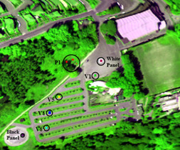
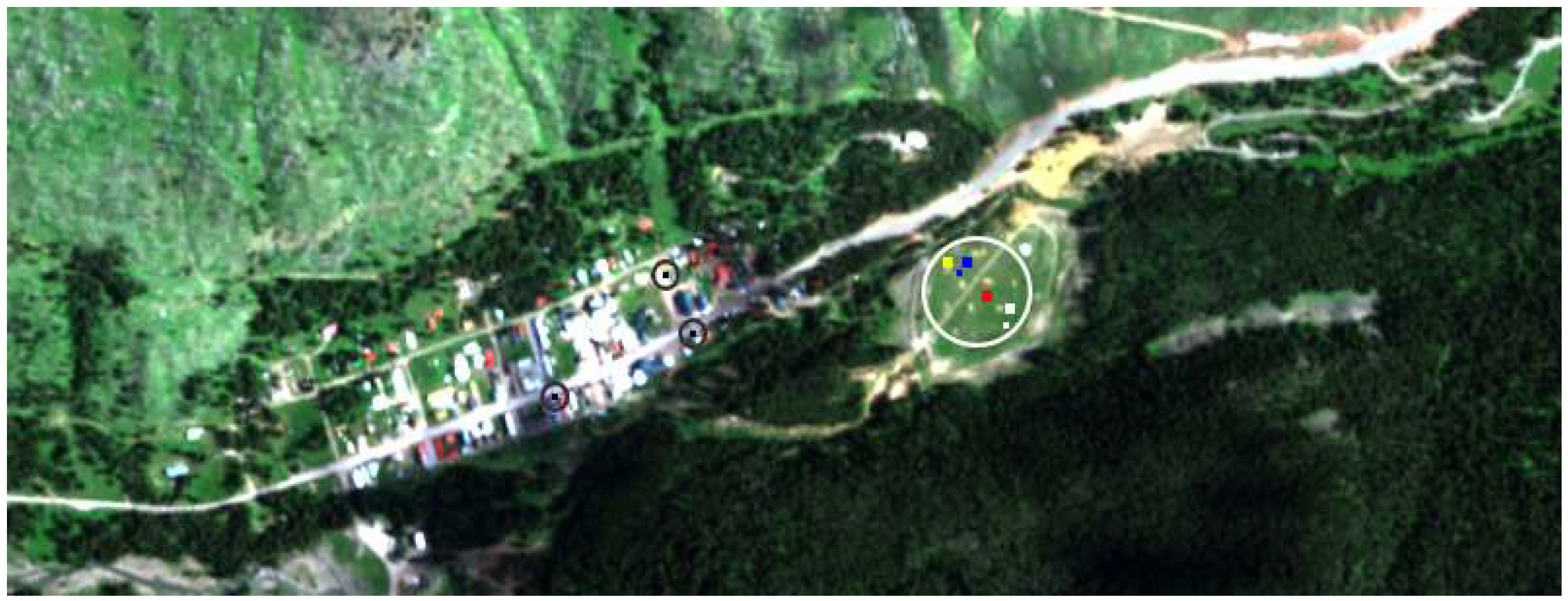
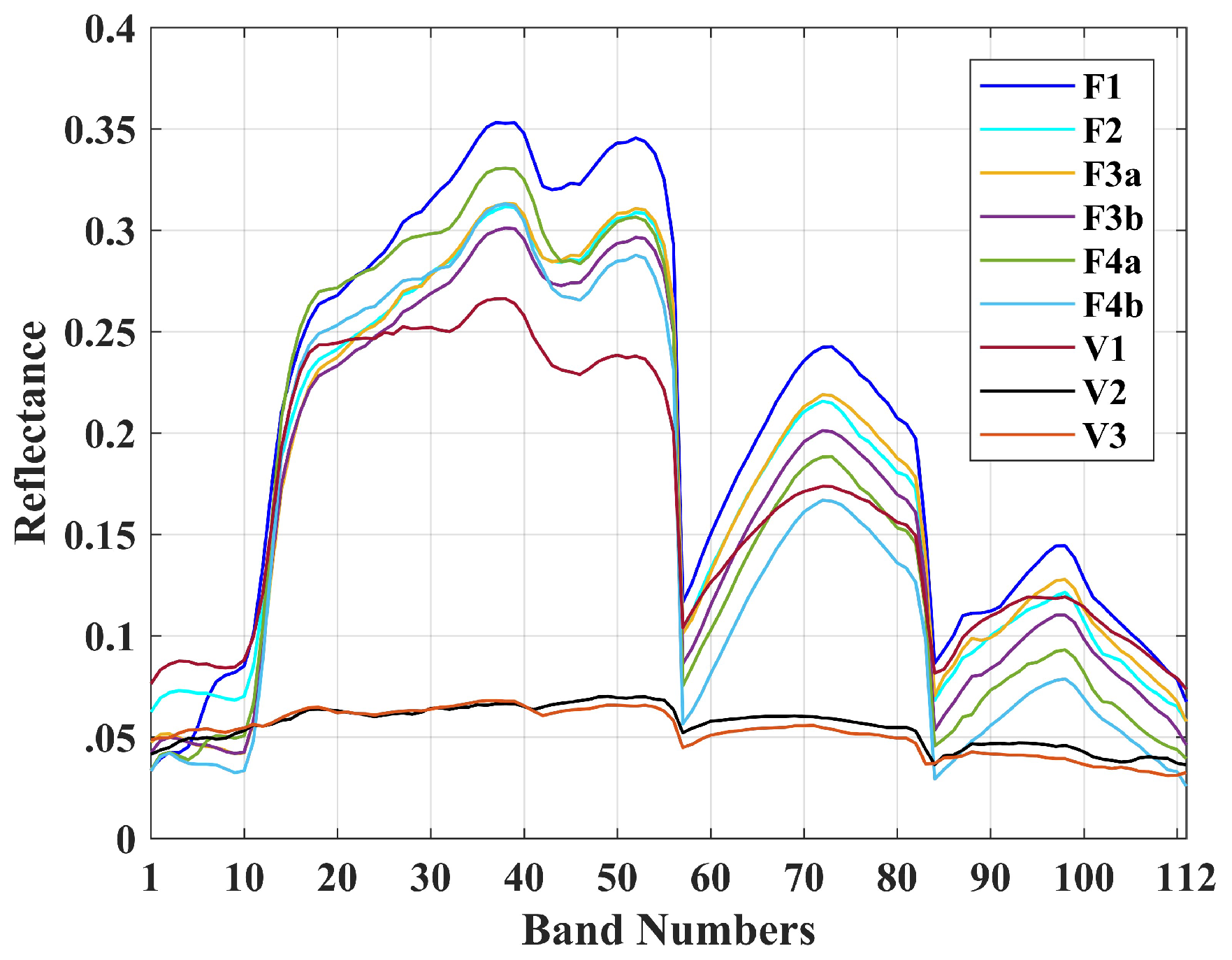
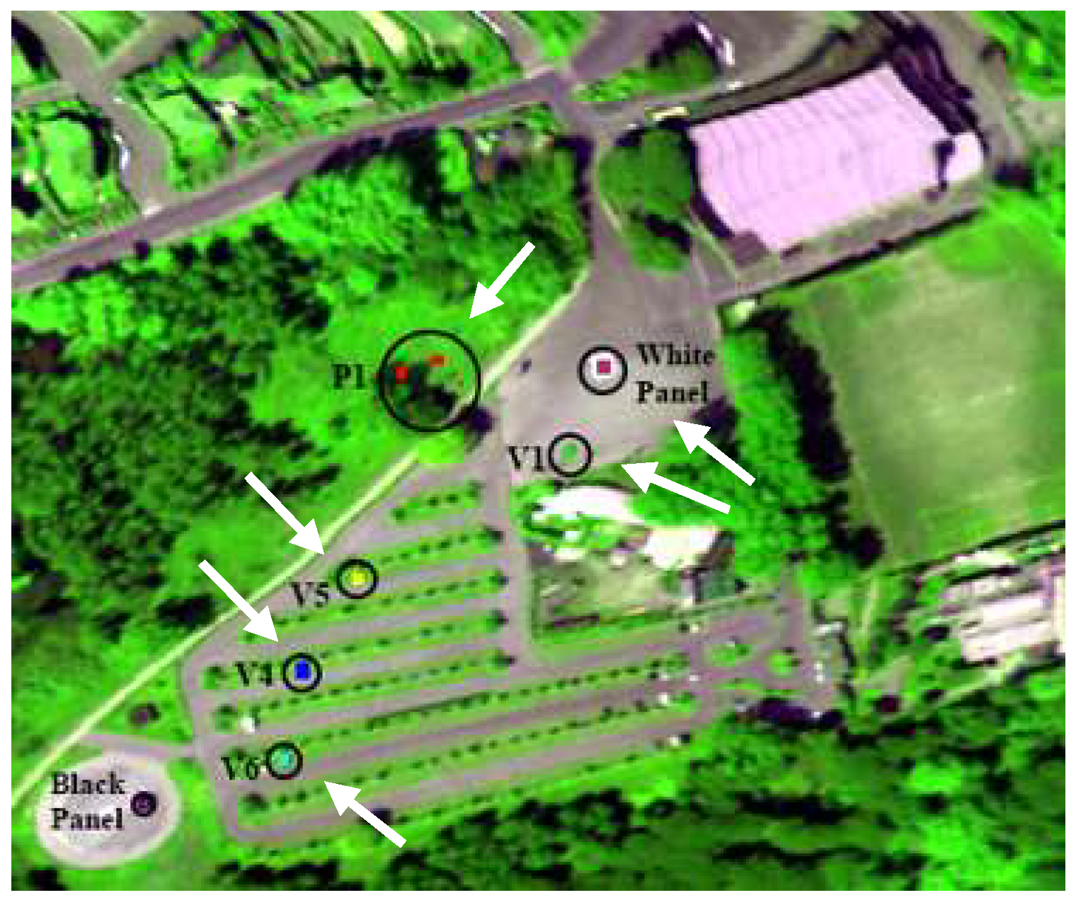
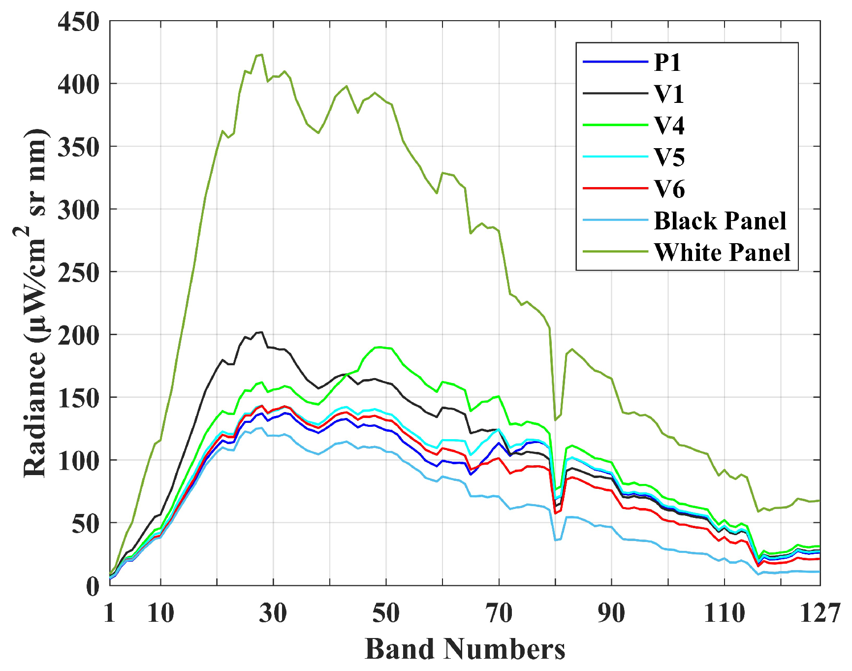
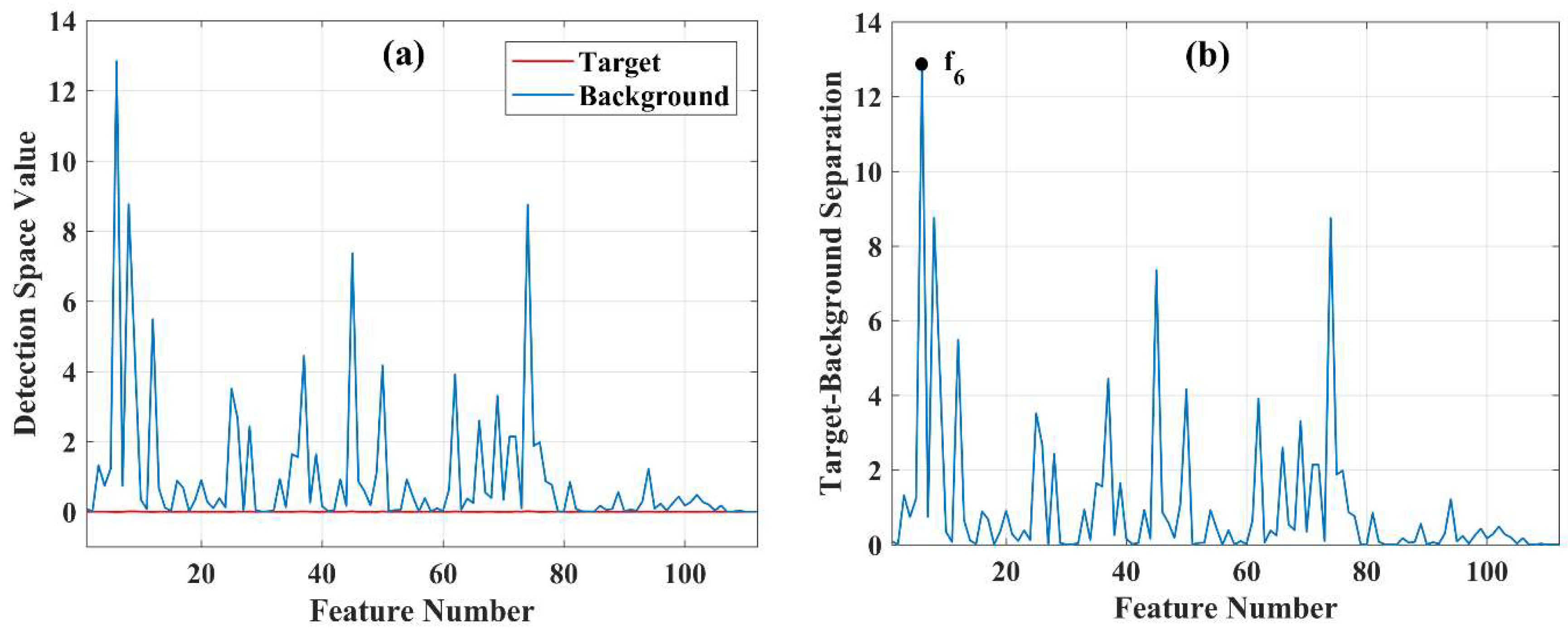
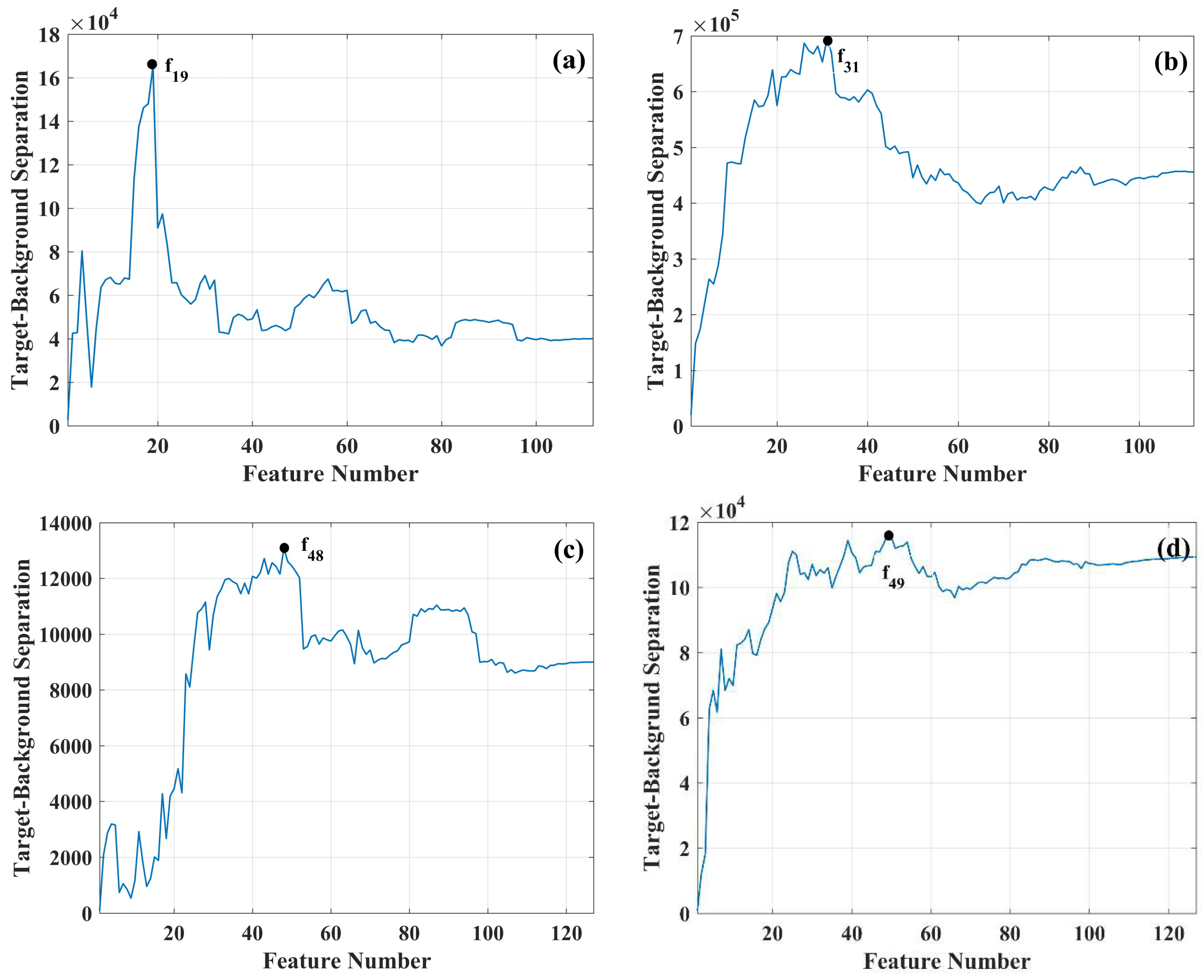
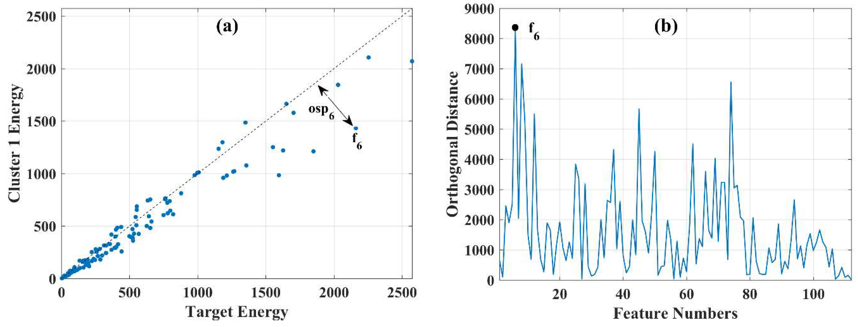
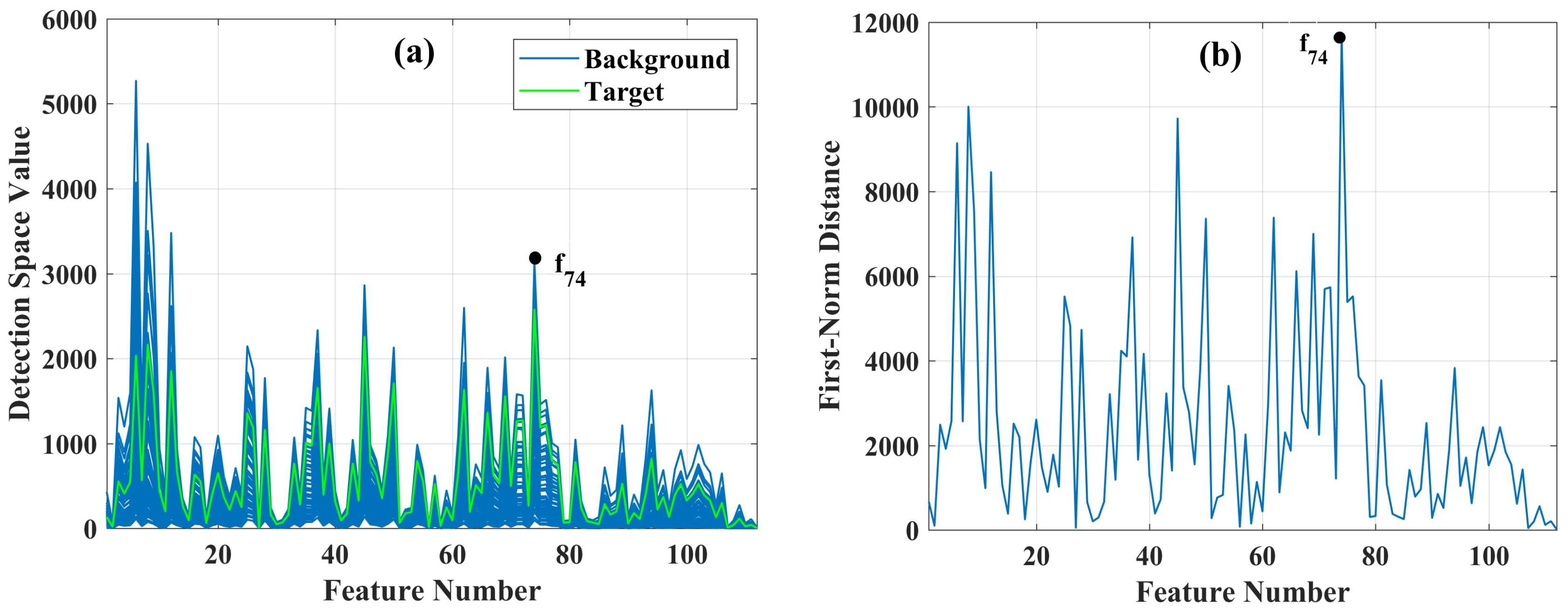
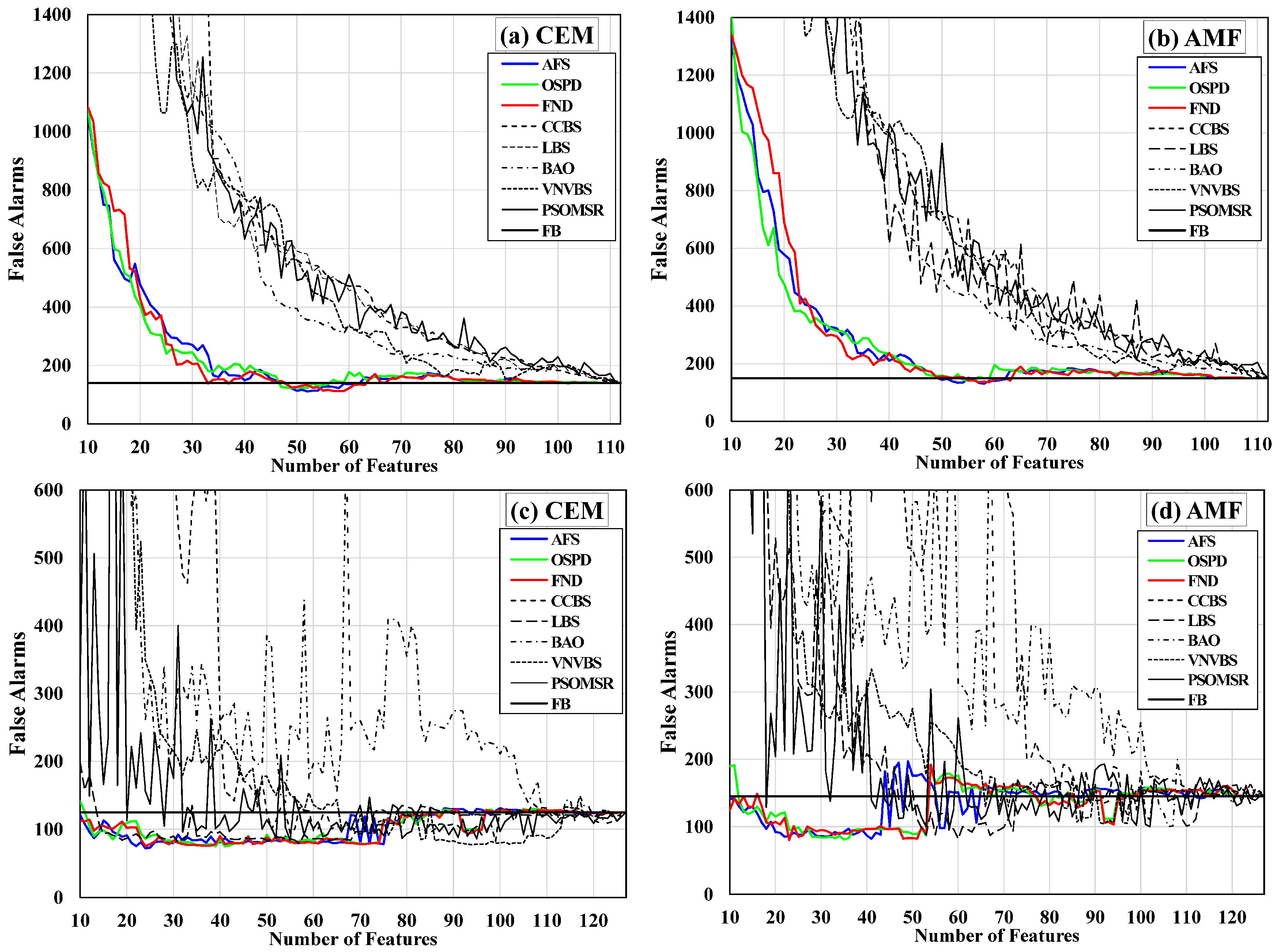
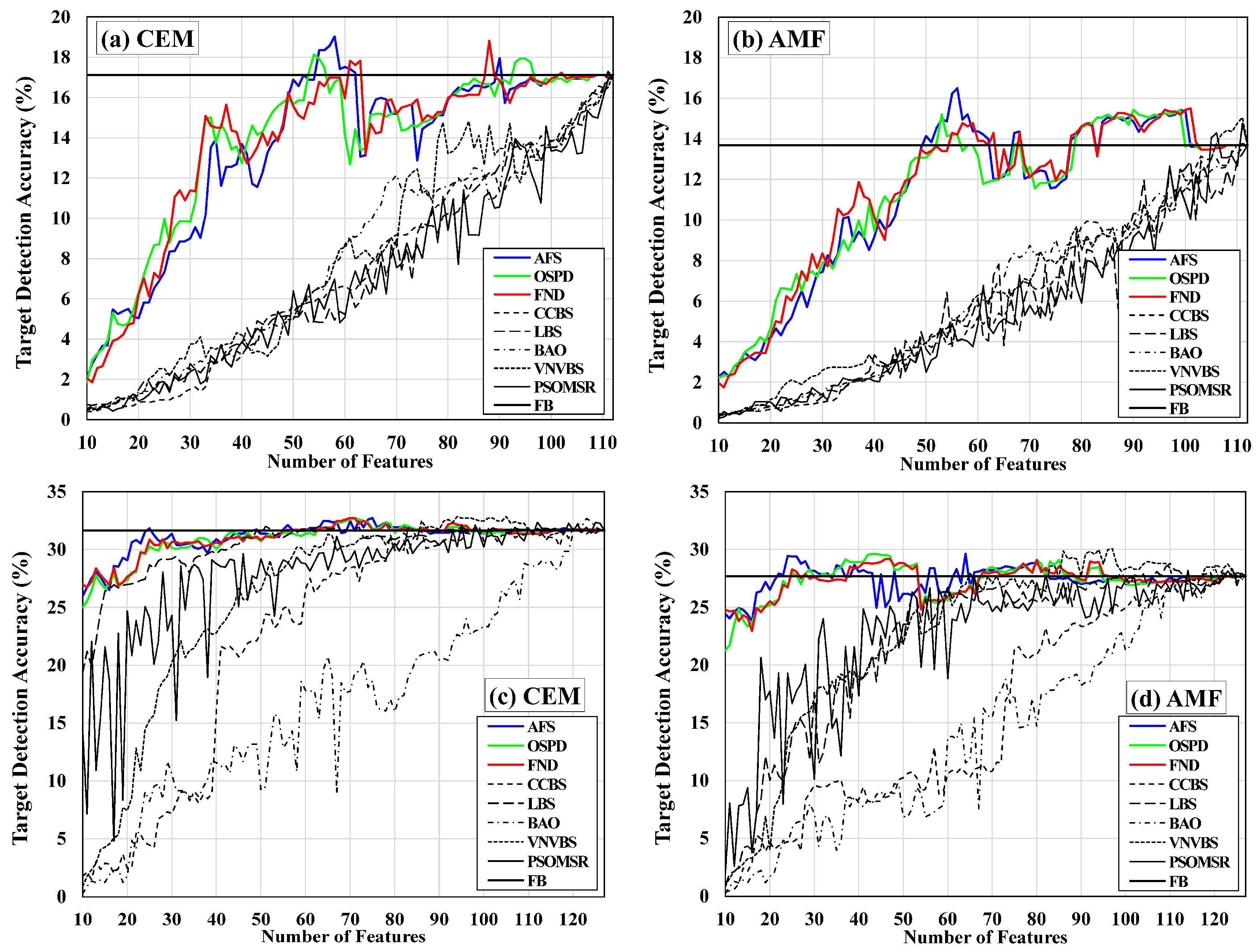
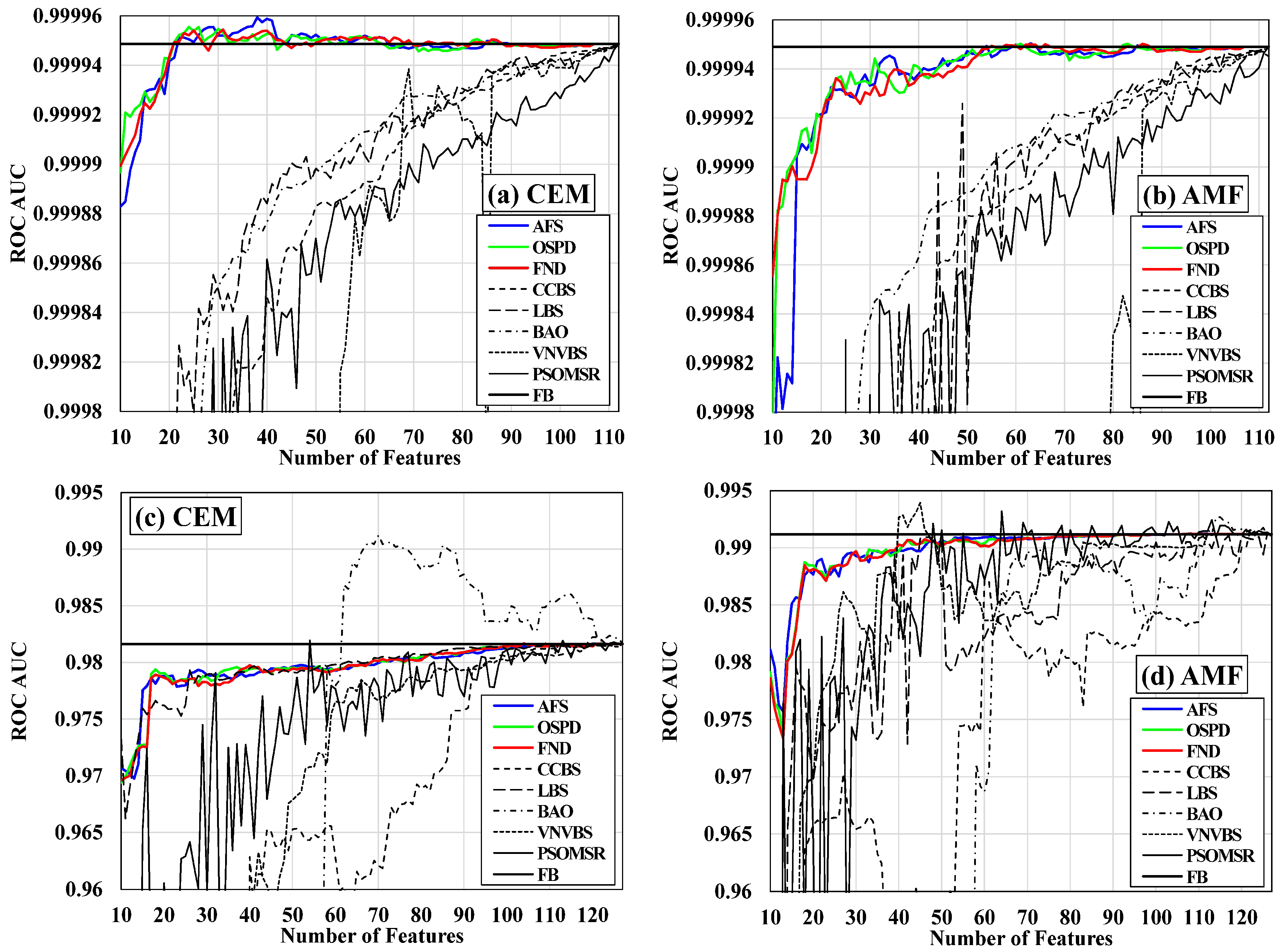
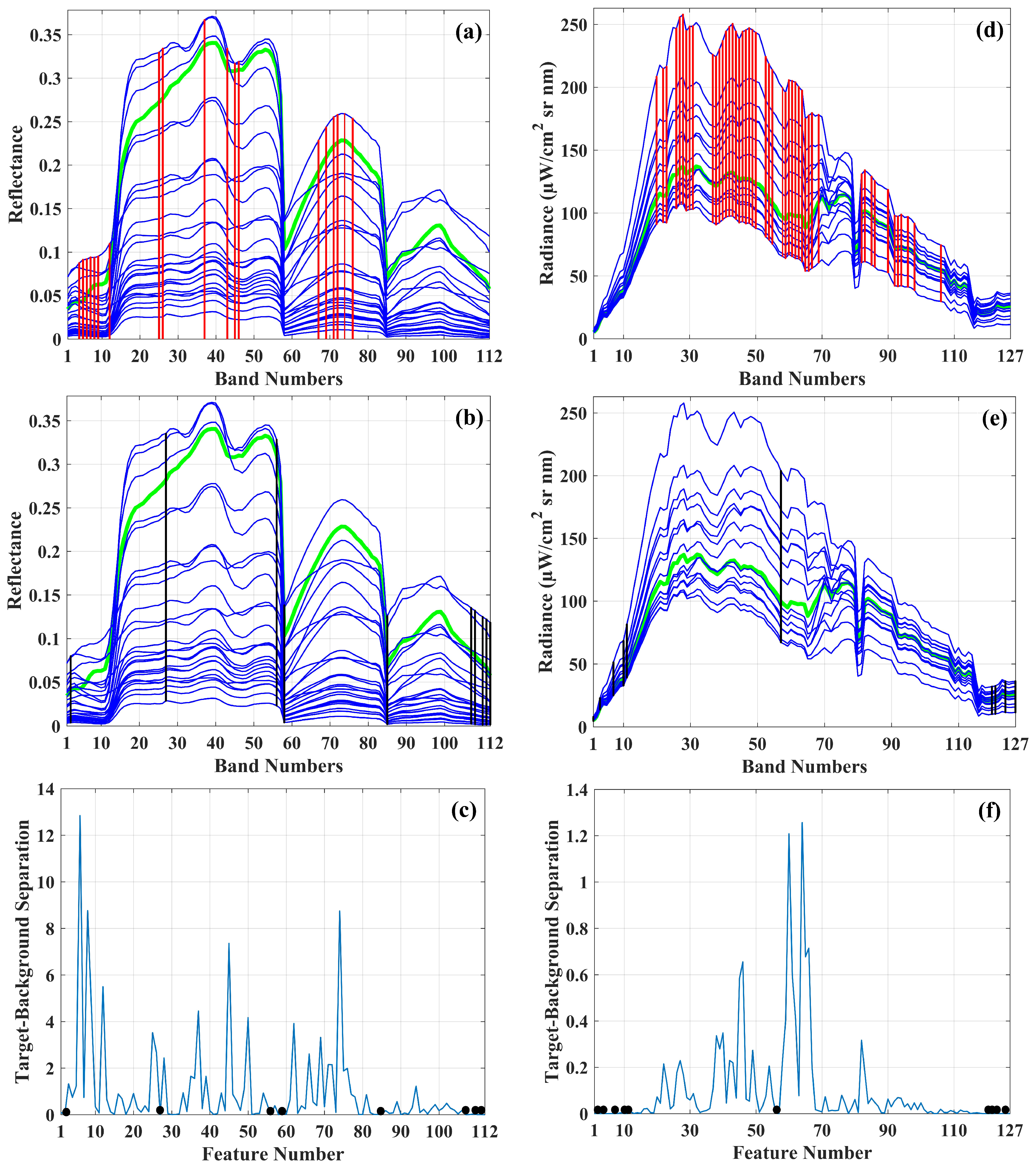
Table 1.
Details of the fabric panels and vehicles used as targets in the HyMap dataset.
| Names | Materials and Sizes | Number of Pixels |
|---|---|---|
| F1 | 3 m Red Cotton Panel | 9 |
| F2 | 3 m Yellow Nylon Panel | 9 |
| F3a | 2 m Blue Cotton Panel | 9 |
| F3b | 1 m Blue Cotton Panel | 1 |
| F4a | 2 m Red Nylon Panel | 9 |
| F4b | 1 m Red Nylon Panel | 1 |
| V1 | 1993 Chevy Blazer | 1 |
| V2 | 1997 Toyota T100 | 1 |
| V3 | 1985 Subaru GL Wagon | 1 |
Table 2.
Details of the panels and vehicles used as targets in the SIM.GA dataset.
| Names | Number of Pixels |
|---|---|
| P1 | 44 |
| Black Panel | 4 |
| White Panel | 36 |
| V1 | 20 |
| V4 | 42 |
| V5 | 25 |
| V6 | 20 |
Table 3.
Total false alarms (TFA) and the corresponding total true positives (TTP) achieved by the feature selection (FS) methods based on the maximum target detection accuracy (TDA%). NT is the total number of targets. #F is the number of optimal features. TNS indicates the total negative score for each FS method.
| Detector | Existing Feature Selection Methods | Proposed Feature Selection Methods | FB | |||||||||
|---|---|---|---|---|---|---|---|---|---|---|---|---|
| CCBS | LBS | BAO | VNVBS | PSOMSR | AFS | OSPD | FND | |||||
| TFA | TFA | TFA | TFA | TFA | TFA | TFA | TFA | TFA | ||||
| TTP | TTP | TTP | TTP | TTP | TTP | TTP | TTP | TTP | ||||
| TDA% | TDA% | TDA% | TDA% | TDA% | TDA% | TDA% | TDA% | TDA% | ||||
| #F | #F | #F | #F | #F | #F | #F | #F | #F | ||||
| Dataset | HyMap NT = 41 | CEM | 140 | 144 | 140 | 140 | 140 | 122 | 130 | 145 | 140 | |
| 31 | 32 | 31 | 31 | 31 | 31 | 31 | 35 | 31 | ||||
| 17.13 | 17.3 | 17.13 | 17.13 | 17.13 | 19.02 | 18.13 | 18.82 | 17.13 | ||||
| 112 | 111 | 112 | 112 | 112 | 58 | 54 | 88 | 112 | ||||
| AMF | 149 | 155 | 148 | 165 | 169 | 147 | 160 | 159 | 149 | |||
| 26 | 26 | 26 | 31 | 31 | 31 | 31 | 31 | 26 | ||||
| 13.68 | 13.27 | 13.76 | 15.05 | 14.76 | 16.49 | 15.42 | 15.5 | 13.68 | ||||
| 112 | 111 | 111 | 111 | 111 | 56 | 90 | 101 | 112 | ||||
| TNS | 314 | 323 | 313 | 325 | 329 | 289 | 310 | 320 | 314 | |||
| SIM.GA NT = 191 | CEM | 109 | 84 | 109 | 80 | 112 | 78 | 78 | 78 | 125 | ||
| 96 | 88 | 98 | 89 | 98 | 88 | 88 | 88 | 100 | ||||
| 32 | 32 | 32.67 | 32.84 | 32.34 | 32.71 | 32.71 | 32.71 | 31.65 | ||||
| 98 | 51 | 123 | 105 | 125 | 75 | 71 | 70 | 127 | ||||
| AMF | 158 | 149 | 134 | 105 | 153 | 106 | 96 | 97 | 145 | |||
| 98 | 90 | 93 | 89 | 97 | 88 | 85 | 84 | 93 | ||||
| 28.08 | 27.94 | 28.62 | 30.07 | 28.2 | 29.63 | 29.62 | 29.17 | 27.68 | ||||
| 119 | 126 | 120 | 97 | 114 | 64 | 43 | 46 | 127 | ||||
| TNS | 455 | 437 | 434 | 389 | 452 | 390 | 383 | 379 | 459 | |||
Table 4.
The time in seconds spent by the feature selection (FS) methods to select optimal features.
Table 4.
The time in seconds spent by the feature selection (FS) methods to select optimal features.
| Existing FS Methods | Proposed FS Methods | ||||||||
|---|---|---|---|---|---|---|---|---|---|
| CCBS | LBS | BAO | VNVBS | PSOMSR | AFS | OSPD | FND | ||
| Dataset | HyMap | 111 | 55 | 3 | 2 | 21,500 | 8 | 2 | 4 |
| SIM.GA | 132 | 53 | 2 | 1 | 11,396 | 9 | 1 | 3 | |
Table 5.
The first twenty optimal features selected by the proposed methods for the first target.
| Dataset | FS Method | Selected Features |
|---|---|---|
| HyMap | AFS | 26 25 6 8 4 5 69 74 76 72 71 45 46 67 12 9 43 7 37 13 |
| OSPD | 8 6 5 4 69 74 76 67 72 71 12 9 45 49 25 28 26 43 35 37 | |
| FND | 72 69 8 6 4 5 67 71 12 9 45 48 74 25 28 26 43 35 37 49 | |
| SIMGA | AFS | 65 60 58 64 59 45 61 38 66 27 46 40 62 54 43 82 94 49 67 39 |
| OSPD | 65 61 64 58 60 59 45 38 66 26 62 46 40 54 39 43 67 49 23 22 | |
| FND | 61 65 64 58 60 59 45 38 66 26 62 46 40 54 63 43 39 67 23 22 |
Table 6.
The last ten features selected by AFS.
| AFS | HyMap | 85 111 2 108 58 110 56 27 107 112 |
| SIMGA | 1 10 121 7 124 57 3 11 127 120 |
© 2019 by the authors. Licensee MDPI, Basel, Switzerland. This article is an open access article distributed under the terms and conditions of the Creative Commons Attribution (CC BY) license (http://creativecommons.org/licenses/by/4.0/).
Share and Cite
MDPI and ACS Style
Moeini Rad, A.; Abkar, A.A.; Mojaradi, B. Supervised Distance-Based Feature Selection for Hyperspectral Target Detection. Remote Sens. 2019, 11, 2049. https://0-doi-org.brum.beds.ac.uk/10.3390/rs11172049
AMA Style
Moeini Rad A, Abkar AA, Mojaradi B. Supervised Distance-Based Feature Selection for Hyperspectral Target Detection. Remote Sensing. 2019; 11(17):2049. https://0-doi-org.brum.beds.ac.uk/10.3390/rs11172049
Chicago/Turabian StyleMoeini Rad, Amir, Ali Akbar Abkar, and Barat Mojaradi. 2019. "Supervised Distance-Based Feature Selection for Hyperspectral Target Detection" Remote Sensing 11, no. 17: 2049. https://0-doi-org.brum.beds.ac.uk/10.3390/rs11172049
Note that from the first issue of 2016, this journal uses article numbers instead of page numbers. See further details here.