Synergy of Satellite, In Situ and Modelled Data for Addressing the Scarcity of Water Quality Information for Eutrophication Assessment and Monitoring of Swedish Coastal Waters

Abstract

Monthly CHL-a and Secchi Depth (SD) data derived from the full mission data of the Medium Resolution Imaging Spectrometer (MERIS; 2002–2012) were analysed along a horizontal transect from the inner Bråviken bay and out into the open sea. The CHL-a values were calibrated using an algorithm derived from Swedish lakes. Then, calibrated Chl-a and Secchi Depth (SD) estimates were extracted from MERIS data along the transect and compared to conventional monitoring data as well as to data from the Swedish Coastal zone Model (SCM), providing physico-biogeochemical parameters such as temperature, nutrients, Chlorophyll-a (CHL-a) and Secchi depth (SD). A high negative correlation was observed between satellite-derived CHL-a and SD (ρ = −0.91), similar to the in situ relationship established for several coastal gradients in the Baltic proper. We also demonstrate that the validated MERIS-based estimates and data from the SCM showed strong correlations for the variables CHL-a, SD and total nitrogen (TOTN), which improved significantly when analysed on a monthly basis across basins. The relationship between satellite-derived CHL-a and modelled TOTN was also evaluated on a monthly basis using least-square linear regression models. The predictive power of the models was strong for the period May-November (R²: 0.58–0.87), and the regression algorithm for summer was almost identical to the algorithm generated from in situ data in Himmerfjärden bay. The strong correlation between SD and modelled TOTN confirms that SD is a robust and reliable indicator to evaluate changes in eutrophication in the Baltic proper which can be assessed using remote sensing data. Amongst all three assessed methods, only MERIS CHL-a was able to correctly depict the pattern of phytoplankton phenology that is typical for the Baltic proper. The approach of combining satellite data and physio-biogeochemical models could serve as a powerful tool and value-adding complement to the scarcely available in situ data from national monitoring programs. In particular, satellite data will help to reduce uncertainties in long-term monitoring data due to its improved measurement frequency.

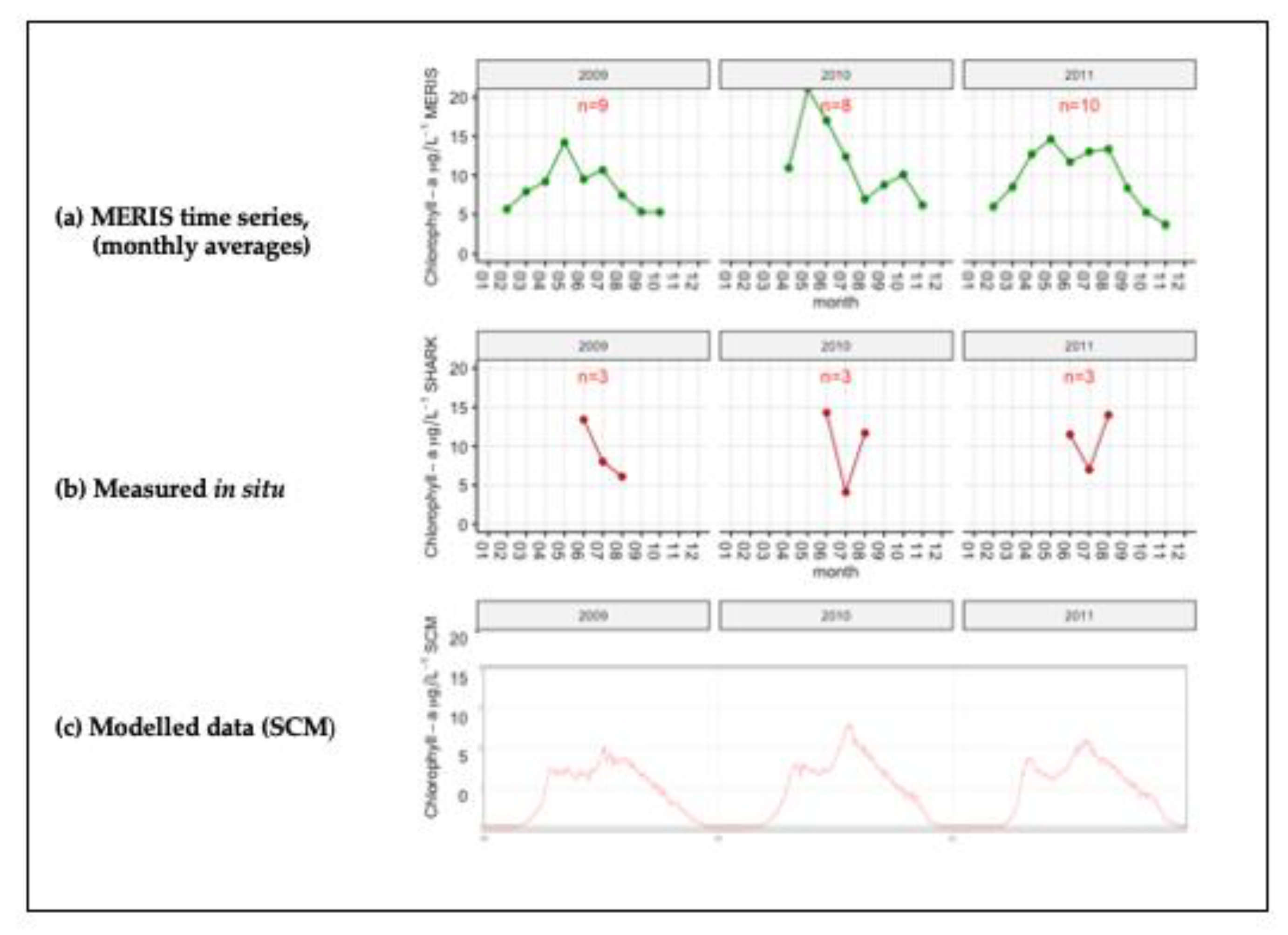
1. Introduction

Eutrophication is a process of increased production of organic matter in the waterbody, which is stimulated by increased availability of inorganic nitrogen (N) and phosphorus (P) [1]. In the Baltic Sea eutrophication is recognized as a major large-scale environmental pressure, partially attributed to an excess loading of anthropogenically-derived nutrients [2,3,4]. In marine systems, eutrophication occurs predominantly in coastal areas and semi-enclosed waterbodies [2,5,6]. Nutrient loads to coastal areas have significantly increased in recent decades due to population growth especially in coastal areas. In the Baltic Sea the problem is exalted due to the relatively large catchment area of the Baltic Sea (i.e., 4.2 times the Baltic Sea), and a relatively low water exchange rate with the North Sea. For the last three decades, it is has been acknowledged that excessive amounts of nutrients such as N, P and organic matter—often represented by organic particular carbon (POC)—result in anoxic bottom waters, the spreading of dead bottom zones and increased frequency and intensity of algal blooms [7,8,9,10,11].

In coastal areas, nutrient enrichment frequently correlates with an increase in phytoplankton primary production and phytoplankton biomass—bringing about eutrophic conditions—and decreasing the light penetration through the water column. Usually, CHL-a is used as an indicator for phytoplankton biomass [12] and Secchi depth (SD)—a measure of water transparency—can be used as an indicator of eutrophication as the increase of phytoplankton biomass has a substantial influence on water clarity [2,13]. Thus, CHL-a and SD measurements—besides being the most common measurements in oceanography—are often considered key indicators for eutrophication. However, this approach is somewhat misleading due to the influence of Coloured Dissolved Organic Matter (CDOM) and Suspended Particulate Matter (SPM) on Secchi depth [14,15,16].

When considering eutrophication from a regulatory perspective, our ability to assess and measure water quality and ecologically relevant parameters becomes important. For example, the Water Framework Directive (WFD) [17] requires the assessment of the ecological status of all surface water bodies. This includes coastal and transitional waters (e.g., 690 water bodies along the Swedish coast) within the boundary of one nautical mile measured from a pre-defined, coastal baseline [18]. The WFD objective is to achieve a ‘good’ and non-deteriorating status of all waters including coastal water bodies. Each EU member state is responsible for establishing monitoring programs in order to obtain a coherent and comprehensive overview of the water status within each river basin district [17]. For operational monitoring, the WFD requires the frequency for monitoring to be determined by Member States as to provide sufficient data for reliable assessment of the status of the relevant quality element. Furthermore, measurement frequency shall be chosen in order to achieve an acceptable level of confidence and precision [17]. Additionally, sampling frequencies should take into account and minimize the impact of seasonal variation on the results, and thus ensure that the results reflect changes in the water body as a result of changes due to anthropogenic pressure and be monitored during different seasons within the same year, if required, in order to achieve this objective [17]. As an example, according to European guidelines, phytoplankton should be sampled every six months, for a minimum of three years out of a six-year assessment period. However, many coastal areas in Sweden are sampled more frequently (3–5 times) in July and August.

While such frequencies for monitoring may be sufficient for certain waterbodies to assess water quality, they may be less so for more complex systems exposed to combinations of diffuse sources of pressures; outlets from large river catchments with high seasonal variability; and influences from the open sea. To fully capture the variability, monitoring should be performed on a monthly basis throughout the entire season, and if possible weekly sampling during times of phytoplankton blooms. However, the stations that are included in monitoring programs might still not fully capture the spatial and temporal variability of a waterbody [19,20,21]. Moreover, due to costs associated with in situ measurements, CHL-a samples are often taken only during the summer months (e.g., to track the development of the cyanobacterial blooms) once a month. This leaves the remaining seasons unmonitored—not to mention that most of the waterbodies and coastal zones are left completely unmonitored due to the absence of any monitoring efforts [22].

The solution for lack of temporal and spatial coverage of monitoring data in the coastal zone might be found in remote sensing. Specifically, in the past decade, there has been considerable progress in the remote sensing of optically-complex waters such as the Baltic Sea. This was mostly due to the MEdium Resolution Imaging Spectrometer (MERIS) launched by European Space Agency (ESA) on board of ENVISAT satellite in 2002. Due to its better spatial (300 m/pixel) and spectral resolution, i.e., more distinct bands in the visible compared to other ocean colour sensors (such as SeaWiFS or MODIS). MERIS allowed for the monitoring of coastal areas and to derive improved water quality products (CHL-a, SD, Total Suspended Matter/turbidity from Space). Some of the derived remote sensing products are important ecosystem state variables [16,23]. Thus, the 10-year full mission data set from MERIS allows us to investigate the water quality dynamics in coastal areas, to reliably quantify concentrations of CHL-a, to monitor the spatial patterns of SD and to track the extent of river discharge plumes using suspended matter [16,24,25,26]. This type of information allows us to provide data in areas where conventional in situ monitoring efforts do not deliver any measurements. Remote sensing-based estimations of water quality is envisioned to facilitate the implementation of goals set by WFD, Marine Strategy Planning (MSP) and for supporting the assessments done by the Baltic Marine Environment Protection Commission (HELCOM), also known as Helsinki Commission [1,4,13,14].

Besides remote sensing and in situ monitoring data, there are additional sources of water quality assessment available via modelling. The Swedish Meteorological and Hydrological Institute (SMHI), e.g., has developed a coastal zone hydrological model with high temporal resolution (every 10 min) that can be used by water authorities to make adequate water quality assessment [22]. Such models are designed to fill spatial (approximately 9–10 km resolution) and temporal gaps, to identify problems with measurements, support monitoring programs and provide predictive long-term scenarios. Yet, it is not clear how these three sources of information (i.e., satellite-derived, in situ, and model generated) compare and can be combined across spatiotemporal scales in complex coastal waters to assess water quality and identify eutrophic zones.

The aim of this study is to explore the relationship between these three sources of water quality information: satellite, in situ and modelled data, and to define complementary and value-adding synergy effects from the combination of these different approaches for monitoring using Bråviken bay as a case study. We will evaluate how remotely sensed data can be used for monitoring when in situ measurements are either scarce or not available at all, thus filling in the gaps in existing monitoring programs with the ultimate aim to support the eutrophication assessments by HELCOM and status classification adopted through EU Directives. This will help to address the uncertainties in drawing conclusions which may be related to scarcity of monitoring data.

The objectives of this study thus are:

(1)

to evaluate horizontal coastal-open sea gradients of CHL-a and SD derived from MERIS (monthly averages) between 2002–2012 and to validate them against in situ data and to apply a correction if necessary and subsequently,

(2)

to evaluate the results against corresponding water quality parameters derived from the SCM, and

(3)

to investigate the degree of coupling between two sets of independently acquired data—i.e., satellite vs. modelled and thereby to infer information about nutrient status from satellite data.

(4)

Another objective is to assess which of the discussed method is best able to depict changes in phytoplankton phenology.

2. Materials and Methods

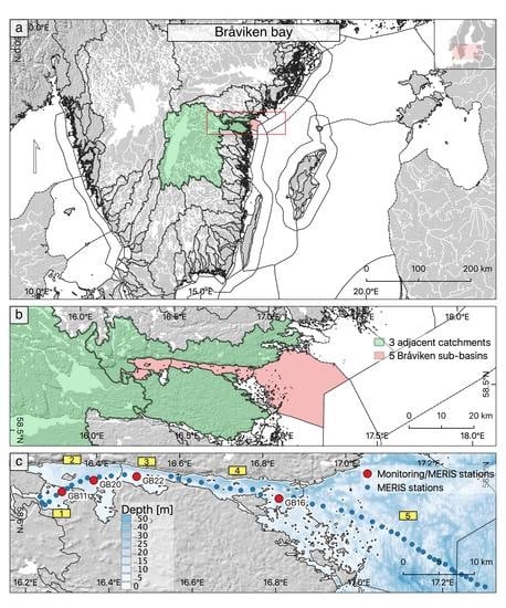
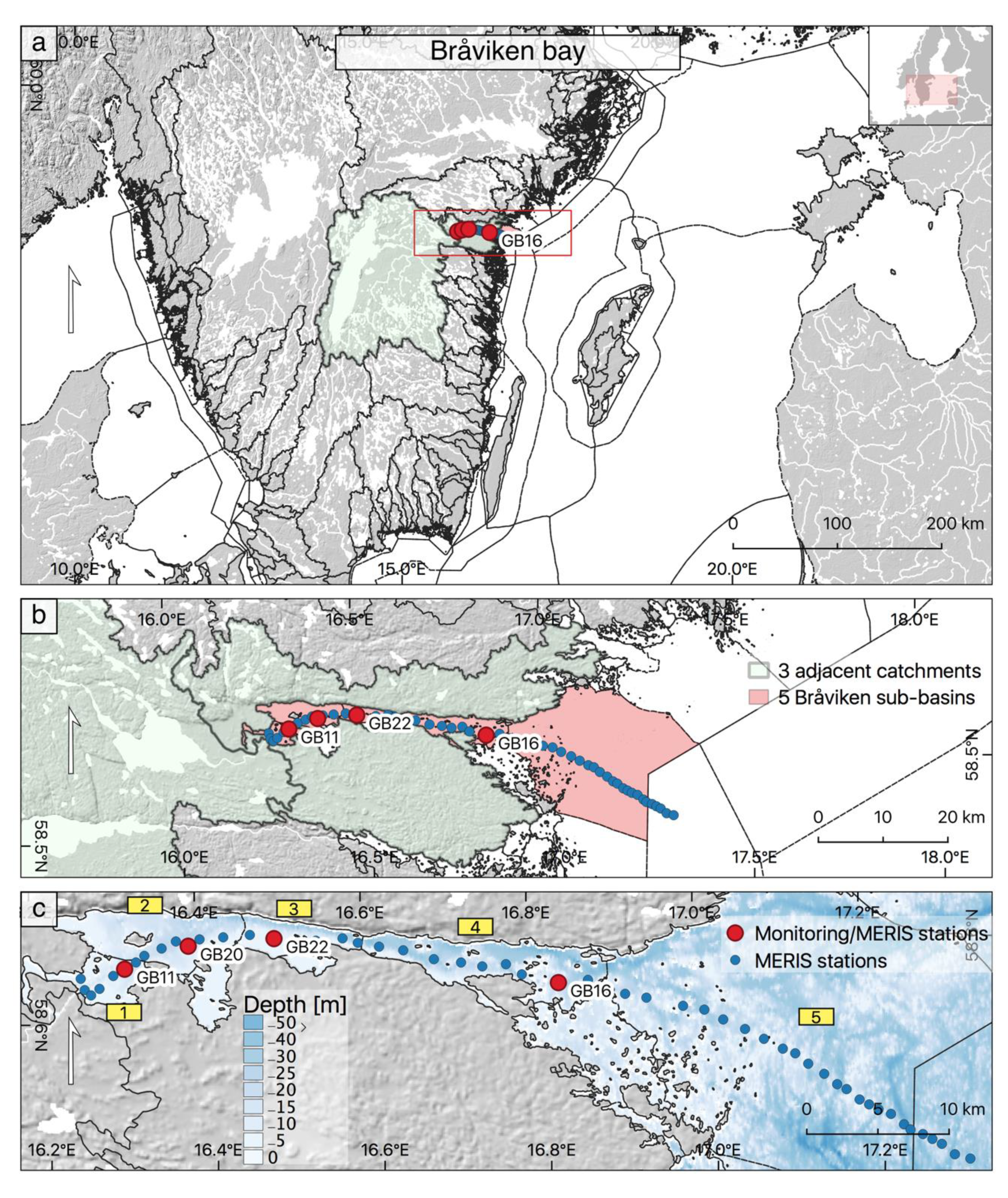
2.1. Area of Investigation

Bråviken (Figure 1) is a narrow, elongated, bay in the northwestern part of the Baltic proper. According to the Swedish Water Archive [27] Bråviken is divided into 5 sub-basins (see Figure 1 and

Table 1. Bråviken waterbodies here listed in the order from the inner-most basin out to the open Baltic along a horizontal transect (Figure 1).

Water Body (no)	Water Body Name in English (In Swedish)	Monitoring Station	No of ‘Pins’ per Waterbody
1	Pampusfjärden (Pampusfjärden)	GB11	7
2	Inner Bråviken (Inre Bråviken)	GB20	6
3	Mid-Bråviken (Mellersta Bråviken)	GB22	5
4	Outer Bråviken (Yttre Bråviken)	GB16	9
5	Bråviken coastal waters (Bråvikens kustvatten)	None	20

): Pampusfjärden (1), Inner Bråviken (2), Mid-Bråviken (3), Outer Bråviken (4), Bråviken’s coastal waters (5). Bråviken is surrounded by one large and two smaller catchments with a total area of 16,470 km². The largest catchment is the drainage basin of Lake Vättern; the second largest lake in Sweden with a surface area of 1912 km² (Figure 1). The catchment contains mostly forest (49%) and agricultural land (18%) as well as water (20%) [28]. Motala river is 100 km long and feeds into Bråviken from Lake Vättern, flowing through one of the richest agricultural areas in Sweden (from Motala to Norrköping). It is the main freshwater contributor to Bråviken. The annual mean water flow to the Baltic Sea from Bråviken is about 100 m³/s [28]. The growth season (sow date to harvest) in the Motala river drainage basin usually starts sometime between early April to early May and lasts, on average, until late September. The discharge point of Motala river is located in the innermost sub-basin of Bråviken—Pampusfjärden—that receives a large freshwater input.

The monitoring stations of the National Monitoring Program are located in each sub-basin (waterbody, Figure 1c) and the monitoring data measured at these stations were used in this study for comparison to MERIS data. A typical horizontal transect along an in-shore to off-shore gradient was chosen using a MERIS scene from Bråviken. The transect was made up of 5–20 pixels in each sub-basin (Table 1). Each pixel location in the transect was marked as a ‘pin’ (i.e., a marker with geographic coordinates on a geo-referenced image referring to a corresponding pixel). Subsequently, all pins were imported into an open source geographic information system (GIS) software for mapping and visualization of geographic data (QGIS 3.0.3-Girona; Figure 1c). The same locations (pins) were then also used for the extraction of water quality constituents (CHL-a and SD) for the 10-year MERIS time-series. The pin extraction process is further explained in Section 2.5 below.

2.2. National Monitoring Data

Swedish National Monitoring data includes various biological and physio-chemical parameters collected at designated stations. For this study, surface CHL-a and SD were downloaded from the national marine environmental monitoring database (SHARKweb [31]) for the monitoring stations GB11, GB20, GB22 and GB16 in Bråviken (Figure 1). Chlorophyll samples were collected at the surface with a Ruttner or rosette sampler and filtered in the lab and subsequently the chlorophyll-a content was determined based on fluorescence measurements [32]. The SD was measured by lowering a white Secchi disk (25 cm in diameter) into the water and noting the water depth (m) at which the disk disappears from the observer’s sight.

2.3. Satellite-Derived Water Quality Data

Medium Resolution Imaging Spectrometer (MERIS) Data Processing

MERIS v.3 data were processed from level 1 to level 2 (L2) using an artificial neural network called ‘Case-2 water processor’ developed by Free University of Berlin, FUB [33]; this L2 processor will be referred to as ‘FUB-processor’ henceforth. The FUB processor is developed for optically-complex waters and has been trained on a range of concentrations of optical properties and corresponding reflectance data. It must be noted that the FUB-processor was developed for coastal waters with a training range of 0–50 μgL⁻¹ for CHL-a, which applies to most Swedish coastal waters. However, for CDOM, the training range of FUB is only from 0.005 m⁻¹ to 1 m⁻¹, which is not sufficient to cover the high CDOM ranges in the inner coastal bays of the Baltic Sea [15,34].

Besides $R_{rs}$ (remote-sensing reflectance) the FUB-processor outputs L2 concentrations of three bio-optical constituents: CHL-a, Total Suspended Matter (TSM) and Coloured Dissolved Organic Matter (CDOM/YEL). The retrieval of these constituents has been validated against in situ measurements in the north-western Baltic Sea during validation campaigns from 2008 and 2010 [35,36] and the FUB performance was assessed [36] with CHL-a overestimated ca. by 27% and TSM underestimated by ca. –27% (compared to sea-truthing data). CHL-a absorption was found to be especially overestimated in inner bays with high CDOM absorption. Additional performance/validation tests were performed using the data from Bråviken which is described in the sections below. Additionally, SD data were generated from remote sensing reflectance ($R_{rs}$) at 490 nm (MERIS channel 3) and 665 nm (MERIS channel 7) using the following local algorithm [37]:

$$\mathrm{SD}=6.55726*e^{\left(-0.8737*\left(\frac{MER7}{MER3}\right)\right)}$$

(1)

Invalid pixels corresponding to land, mixed land and water pixels, various cloud types and cloud buffer as well as coastline were masked out using the following IdePix invalid pixels masking: (LAND, MIXEDPIXEL, CLOUD, CLOUD_SHADOW, CLOUD_BUFFER and COASTLINE; [38,39,40]. Note that no specific ice screening has been performed, and thus high reflectance in spring due to snow on ice may falsely lead to high concentrations of CHL-a.

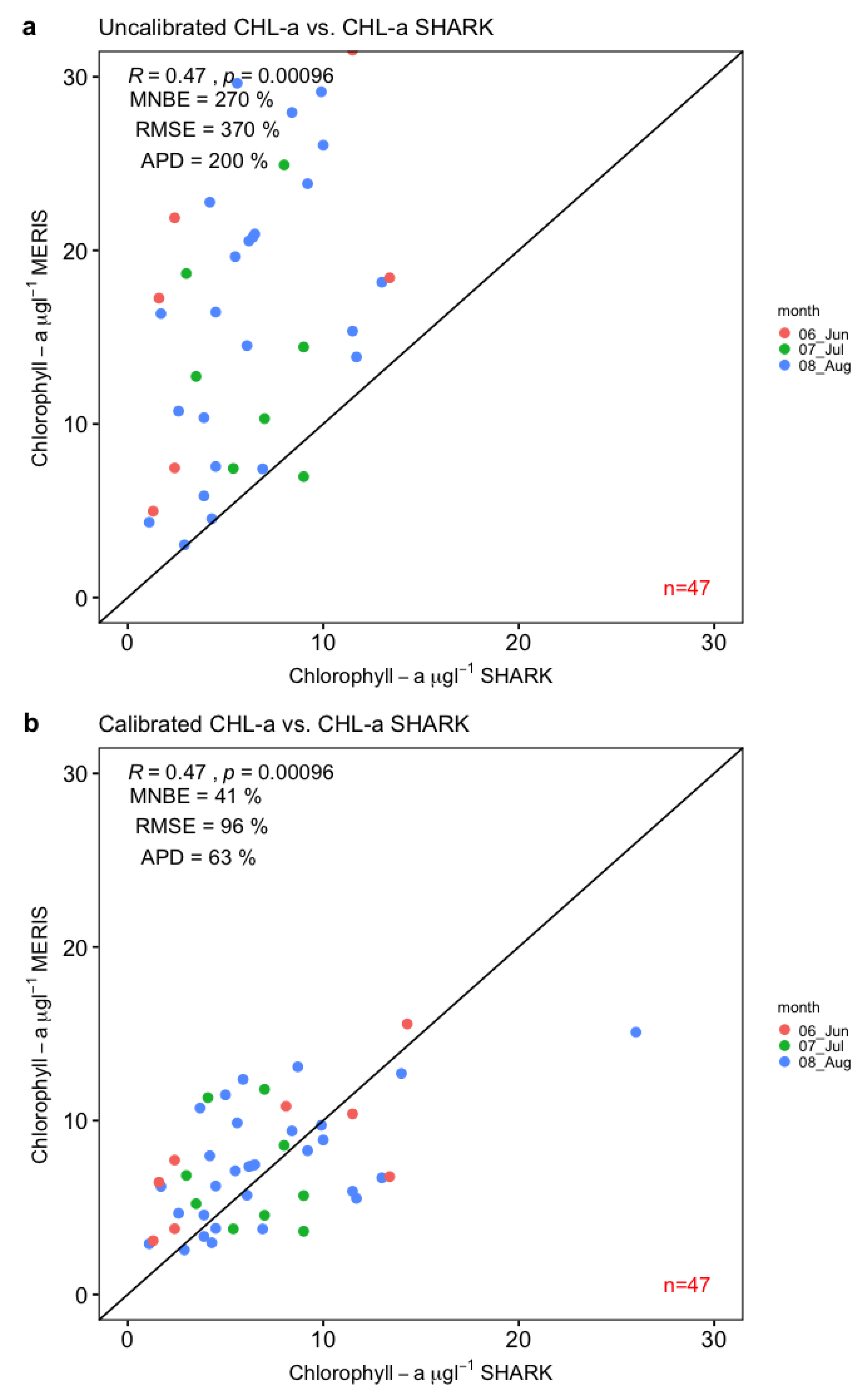
2.4. Application of a Calibration Algorithm for MERIS CHL-a Data Derived from FUB

Previous satellite estimates (FUB-processor) generated CHL-a products in good correspondence with existing in situ data, both in Baltic Sea coastal areas and in Lake Vänern [20,35,36,41]. Further investigations using data from the Swedish great lakes Vänern, Vättern and Mälaren as well as from lake Hjälmaren showed that the FUB-derived CHL-a data performed well in these Swedish lakes when compared to in situ measurements, with a high coefficient of determination (R² = 0.70, [41]). However, the regression line clearly deviated from the 1:1 line, indicating a systematic error. The derived regression model was:

Calib_CHL = 0.2744 × FUB_CHL + 1.7345

(2)

This Swedish lake regression model was then applied to calibrate a time-series of CHL-a data derived from MERIS data in Lake Vänern (using the FUB-processor), and showed good agreement when compared to satellite data [41]. In this study we applied the same calibration algorithm with the assumption that the optical case 2 waters in Bråviken are optically similar to those in Lake Vänern [24,41,42].

The following sections explains the nature of the modelling data (2.4) and how the satellite-derived data (i.e., uncalibrated CHL-a, calibrated CHL-a and SD data) was compared to monitoring and modelled data (2.5).

2.5. Derived Water Quality Estimates from the Swedish Coastal Zone Model (SCM)

The Swedish Meteorological and Hydrological Institute (SMHI) has developed a model system, consisting of a hydrological model called Hydrological Predictions for the Environment Sweden (S-HYPE, [43]) and the Swedish Coastal zone Model (SCM). These two coupled models allow us to derive water quality calculations in lakes, rivers and coastal waters around Sweden. SMHI provides the users with daily, monthly and yearly parameters such as Discharge (Q), Total Nitrogen (TOTN), Nitrate (NO₃), Ammonium (NH₄), Total Phosphorus (TOTP) and Phosphate (PO₄). The SCM delivers physical and bio-geochemical parameters such as water temperature, CHL-a, water turn-over time (days) as well as Secchi depth (SD). The model calculates the vertical profiles of all its variables and assumes that these variables are horizontally homogeneous within the defined water bodies. The sub-basins are identical to the defined national water body classification according to the EU WFD and are described by their hypsographical curve [44]. Recently, the SCM was used to simulate and describe coastal nutrient retention around Sweden [45], and had previously been used for a similar study in the Stockholm archipelago [46]. Both studies have shown that SCM skill to calculate the average state (average vertical profiles and mean seasonal variations) in coastal water bodies is usually good, or acceptable.

For this current study we apply the same cost function (for the same type of data distributions) as in the previous studies [45,46] to evaluate the proximity of the average model states to the average of in situ measurements at three locations in Bråviken. The proximity is evaluated by normalizing the bias between model (P) to observations (O) with the standard deviation of the observations, i.e.,

$$\mathrm{C}=\frac{{{\displaystyle \sum }}_{\mathrm{i}=1}^{\mathrm{n}}\left|\frac{{\mathrm{P}}_{\mathrm{i}}-{\mathrm{O}}_{\mathrm{i}}}{\mathrm{std}\left({\mathrm{O}}_{\mathrm{i}}\right)}\right|}{\mathrm{n}}$$

(3)

where i is a point of comparison. If the average model results fall within the standard deviation of what is observed, C will be below 1. The evaluation covers the years 2002–2012 in the inner and outer Bråviken and also Pampusfjärden. All C values (all three stations and all data types) were below 1. Thus, the SCM performs well at this study site.

2.5.1. Parameterization of CHL-a in the SCM

The CHL-a concentration in SCM is a representation of the modelled phytoplankton (A1, A2 and A3) concentration. The three phytoplankton types are parameterized to function as spring blooming diatoms (A1), smaller summer plankton (A2) and cyanobacteria (A3). The modelled phytoplankton growth is parameterized from light and nutrient availability. The phytoplankton concentrations, and thus CHL-a, decrease as the autotrophs are grazed upon or die. CHL-a concentrations in the SCM thus increase in spring when the phytoplankton has enough light to grow, and decreases in summer if, or when, nutrients are depleted and/or they are grazed upon by zooplankton. Two of the plankton types (A1 and A2) assimilate N and P according to the Redfield ratio, while cyanobacteria (A3) are assumed to be able to use N₂ dissolved in the water, and thus only need to assimilate P.

2.5.2. Parameterization of Secchi Depth in the SCM

The underwater light field in the SCM depends both on the surface irradiance and the attenuation of coastal water. The surface irradiance is calculated from seasonality (incl. e.g., short-wave irradiance, sun angle and the effect of ice) and the light attenuation under water is caused by the attenuation of water itself, the shading of autotrophs and detrital matter and coloured dissolved organic matter (CDOM). The CDOM is parameterized from land-derived dissolved organic nitrogen (DON), which is assumed to be a conservative tracer in the SCM. Secchi depth is calculated from the diffuse attenuation coefficient, K_d, in the 0.5–1 m layer, according to:

$$SD\_SCM=\frac{1.6}{Kd}$$

(4)

2.5.3. Parameterization of Total Nitrogen in the SCM

Total nitrogen (TOTN) in SCM is the sum of inorganic nitrogen (NH4 and NO3), dissolved organic nitrogen (DON), and the nitrogen in particulate organic material, i.e., contained in A1, A2, A3, zooplankton (ZOO) and detrital matter (DET).

TOTN= NH4 + NO3 + DON + (A1 + A2 + A3)_N + (ZOO + DET)_N

(5)

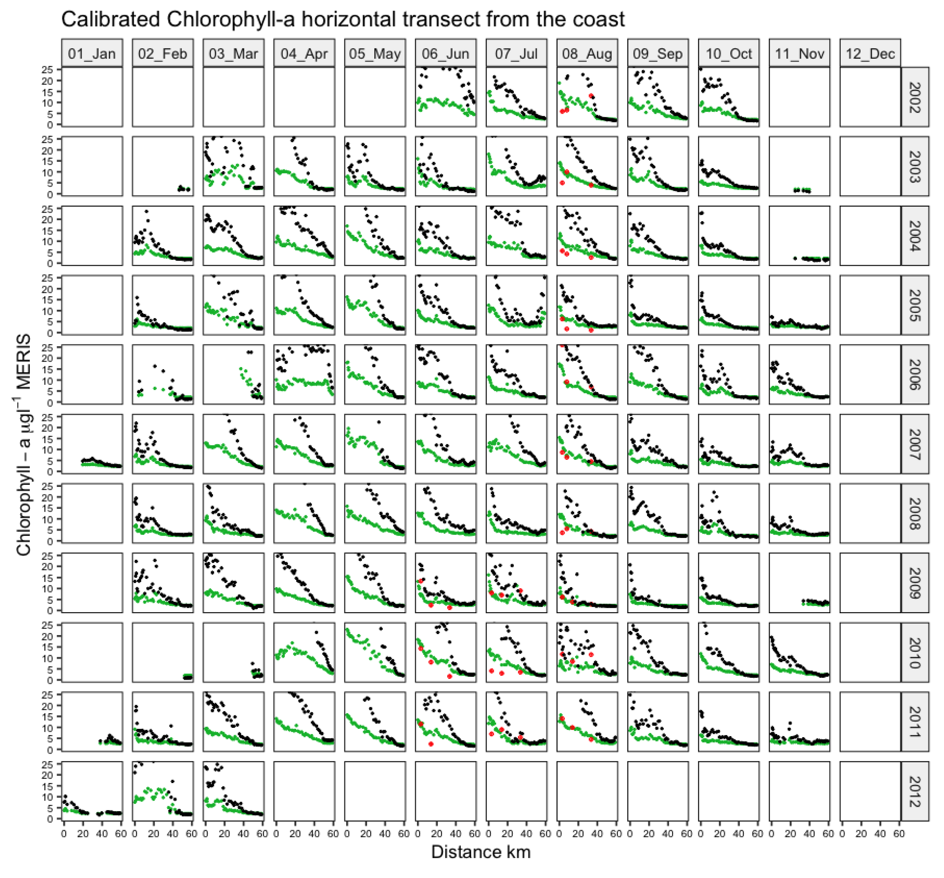
2.6. Horizontal Transects from the Inner Bay out into the Open Sea

CHL-a and SD were both derived from MERIS data and extracted by using a ‘Pixel Extraction’ tool in SentiNel Application Platform (SNAP). All valid pixels available within a 3 × 3 pixel box around the transect stations (a so-called ‘macro pixel’) were extracted from the MERIS data. Hence, each extracted value corresponds to an average of maximum 9 pixels (micropixel) and represents an area of about 1 km². The extracted MERIS transect data were chosen to follow a water quality gradient from the inner bay out into the open sea, including the positions of the monitoring stations. Additional stations located between the monitoring stations, were added to the extracted data, forming a 59 km coastal to open sea transect, starting from the outlet of Motala river.

The full transect consisted of 52 macropixels in total, distributed over the five water bodies as follows: Pampusfjärden—7 macropixels, Inner Bråviken—6 macropixels, Mid-Bråviken—5 macropixels, Outer Bråviken—9 macropixels, Bråviken’s coastal waters—20 macropixels and Open Sea—5 macropixels (Table 1). The macropixel mean values for CHL-a and SD each were plotted against the horizontal distance from the Motala river outlet using the R-package ggpubr [47]. The corresponding available monthly CHL-a and SD data retrieved from SMHI’s SHARKweb database were plotted together with the MERIS-derived horizontal transects in order to visually evaluate the agreement between MERIS and in situ data along the gradient.

The agreement between MERIS and SHARKweb data were also evaluated statistically using 3x3 macropixel windows corresponding to the respective monitoring stations in the SHARKweb data base (in situ data), and using standard metrics as described below in Section 2.6.

In order to compare the MERIS data to the data from the SCM the extracted macropixels within each waterbody were averaged in order to derive an average value (per variable) for each water body. This horizontal transect data (averaged per basin) was then compiled for each month within the 10-year MERIS period (2002–2012), providing a product per basin binned over space and time, and thus corresponding to a L3 product. These L3 data were then analysed and compared to monthly averaged values derived per basin from the SCM model.

2.7. Statistical Analysis

In order to evaluate the agreement between MERIS, SHARKweb and SCM data, the most common metrics used for validation of satellite data were used [36]. The difference between satellite and in situ measurements were quantified statistically (in percent, %) by the Mean Normalized Bias (MNB, Equation (6)) which calculates the systematic bias, the Root-Mean Square Error (RMSE, Equation (7)), indicating the relative error as well as the average Absolute Percentage Difference (APD, Equation (8)), providing the absolute difference between satellite and in situ/modelled data [48,49]. The strength of the correlation was estimated using Spearman’s rank correlation coefficient. The predictive potential between MERIS-derived CHL-a and TOTN for SCM was evaluated fitting least-square regression equation and estimating the coefficient of determination.

$$\left(MNB\right)(\%)=\frac{1}{N}{\displaystyle \sum }_{i=1}^N\left(\frac{Satellit{e}_i-In situ/mode{l}_i}{In situ/mode{l}_i}\right)\times 100$$

(6)

$$\left(RMSE\right)(\%)=\sqrt{\frac{1}{N}{\displaystyle \sum }_{i=1}^N{\left(\frac{Satellit{e}_i-In situ/mode{l}_i}{In situ/mode{l}_i}\right)}^2}\times 100$$

(7)

$$\left(APD\right)(\%)=\exp \left(mean\left|ln\left(\frac{Satellit{e}_i-In situ/mode{l}_i}{In situ/mode{l}_i}\right)\right|\right)-1\times 100$$

(8)

where i is a point of comparison, ($Satellit{e}_i$)_{i=1, N} – MERIS and ($In situ/mode{l}_i$)_{i=1, N} – SHARKweb or SCM, respectively.

3. Results

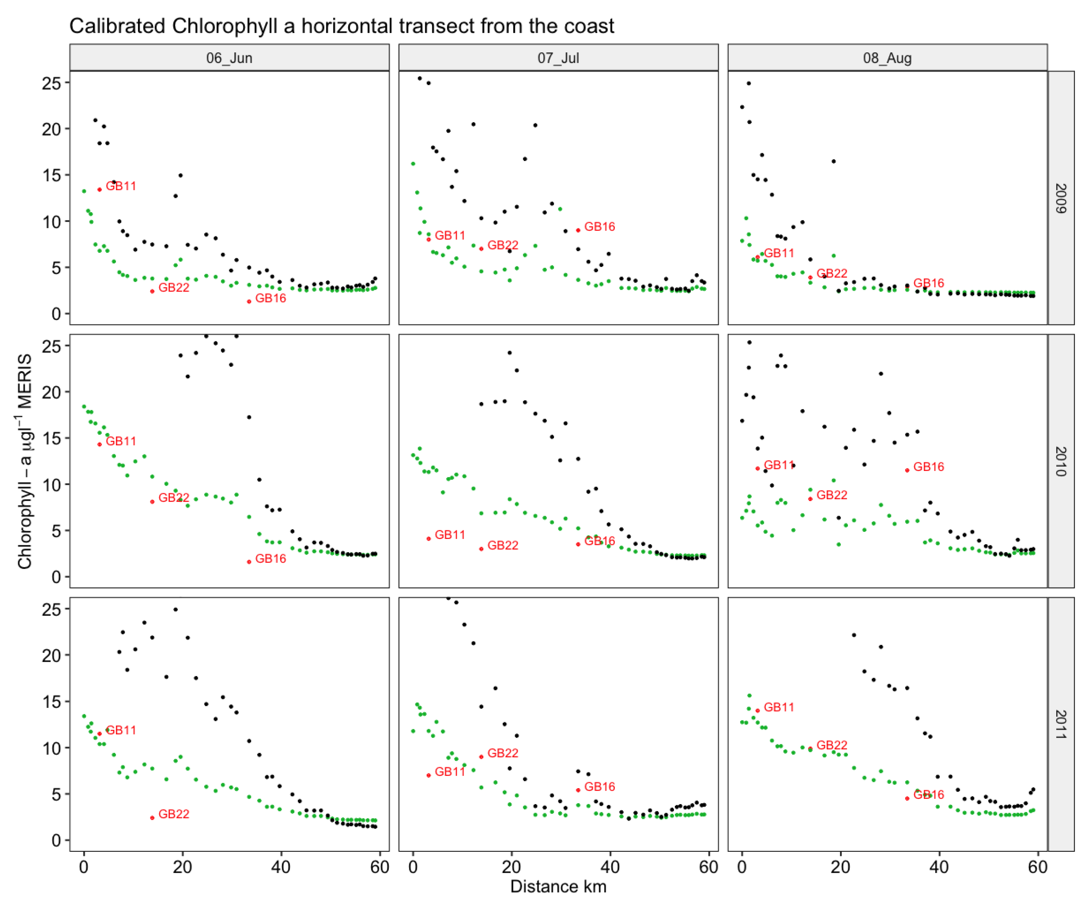
3.1. Horizontal CHL-a Gradients along the Near-Coastal-to-Open Sea Transects

The monthly mean values of the calibrated CHL-a derived for the in situ monitoring stations GB11, GB20, GB22 and GB16 (part of the horizontal MERIS transects) showed 41% MNB, 96% RMS and 63% APD when compared to the SHARKweb in situ point measurements (Figure 1, all available monitoring station throughout Bråviken). This comparison gives an indication how well the in situ samples compare to the monthly means of the respective satellite transect data point before and after applying the calibration algorithm. It indicates that the calibration regression model developed for Swedish lakes improved CHL-a derived from MERIS substantially (Figure 2) also in coastal waters.

CHL-a SHARKweb measurements were available only for June, July and August months from the assessed period 2002–2012. The monthly mean CHL-a concentrations derived from the MERIS archive was plotted with respect to distance from the inner bay out to the open sea (Figure 3). The transect was extracted following the method described in Kratzer and Tett [16]. The article describes and analyses the distribution of bio-optical parameters from the source (inner bay) to the sink (open sea). In the current study, the remote sensing transect thus provides additional CHL-a measurements between monitoring stations, as well for many additional months of the year besides only the summer months (in the case of the SHARKweb in situ database).

Each row in Figure 3 corresponded to the respective year of the MERIS mission (2002–2012) while each column represents the month of year for each year during the MERIS mission. The CHL-a data were plotted before applying the calibration algorithm (black dots) and after calibration (green dots). Additionally, in situ measurements from SHARKweb were plotted along each gradient (red dots) whenever such data were available and illustrated the spatial and temporal discrepancies between MERIS and SHARKweb data.

For the inner Bråviken bay, the mean CHL-a values (calib_CHL) derived from MERIS showed a substantially improved match with in situ data when compared to the uncalibrated values derived from the MERIS FUB-processor. In general, the in situ measurements from Bråviken bay coincide well with the CHL-a transects derived from satellite (calib_CHL), with a few exceptions (see Figure 4; August 2009; June 2010; August 2011) where some in situ data are located below the CHL-a transects derived from MERIS. This was mostly observed in the inner part of Bråviken, where the concentrations of coloured dissolved organic matter are especially high [50]. There is, however, some limitation in comparing data of different temporal scales. In situ measurements taken at one sampling occasion during an entire month may not be the best way of representing the monthly CHL-a concentration for a whole water body (basin) whilst the monthly mean value derived from MERIS data may be closer to the actual mean value. The majority of the points along each transect, however, show good agreement between MERIS and in situ data, and the statistical comparison shown in Figure 2 also confirms that there is relatively good correspondence between the two different data sets, considering that these are optically complex waters. A 3-year sub-set of the full MERIS time-series (2009–2010) is available (Figure 4) during which in situ measurements were measured during all three summer months (June–August). Here, it can be observed that after applying the calibration algorithm (Equation (1)) to the CHL-a concentrations derived from FUB-processed MERIS data, the derived CHL-a values were clearly ‘tuned’ closer to the in situ observations. Amongst this data set, there were some summer months (August 2009, June 2010 and August 2011) during which the calibration algorithm performed especially well.

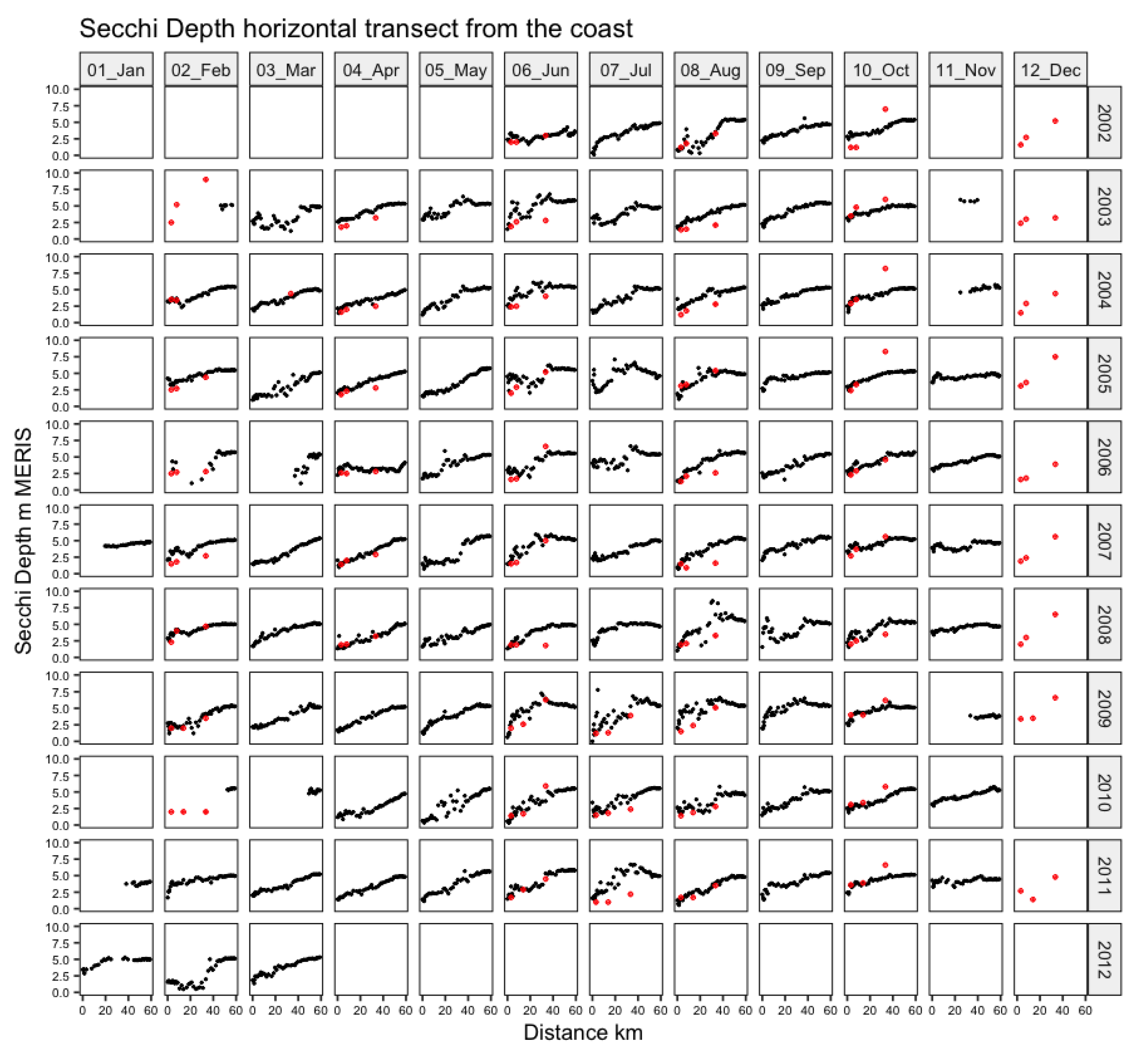
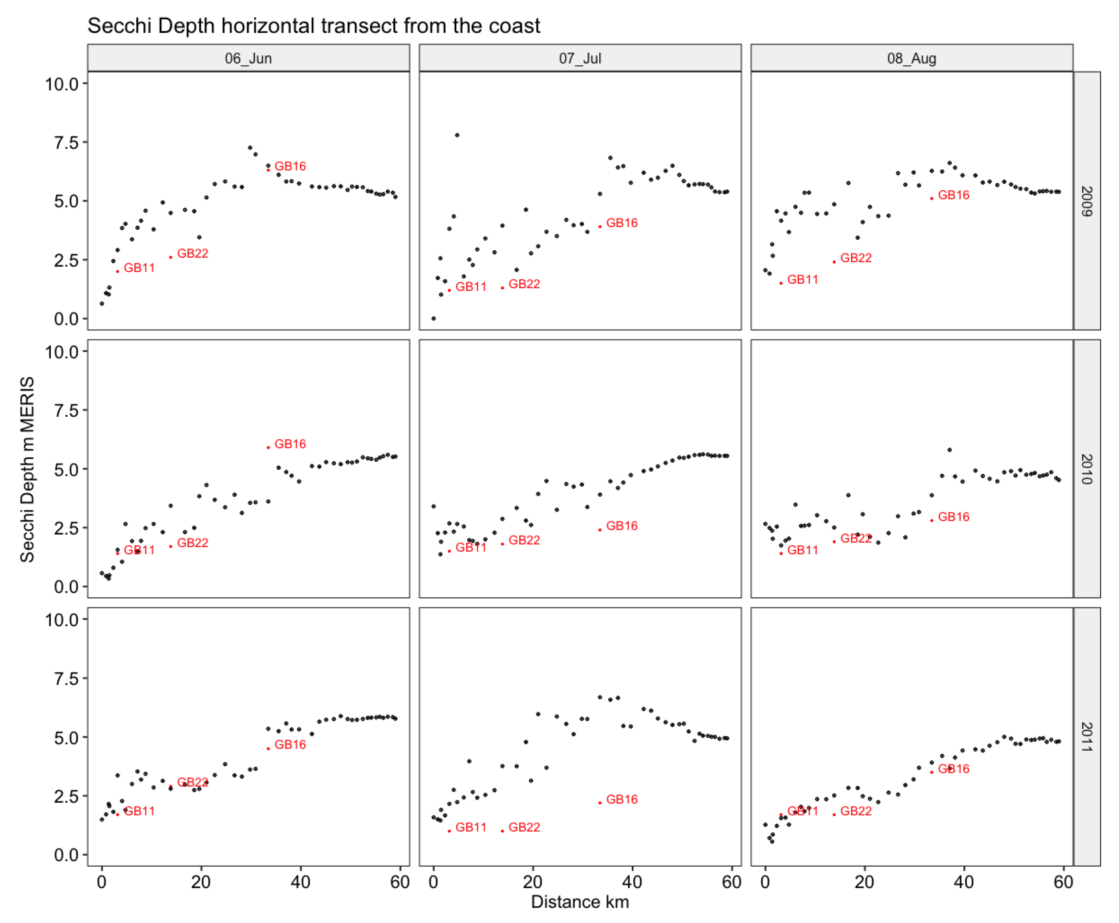
3.2. Horizontal SD Gradients along the Near-Coastal-to-Open Sea Transects

Similarly, Secchi depth (SD) concentrations derived from MERIS FUB were evaluated against SHARKweb data and showed a similar statistical agreement as found between CHL-a (MERIS) and in situ (SHARKweb). SD MERIS had 44% bias (MNB), with a relative error of 73% and 47% APD when compared to data from SHARKweb. SD (SHARKweb) also showed a more abundant temporal frequency, allowing for a comparison not only during the summer months, but also for February, March, April and October (Figure 5).

Further, SD MERIS was plotted against the horizontal distance from the head of Bråviken bay (Figure 6), and visually compared to in situ data. Compared to CHL-a data there were more in situ measurements of SD available and, these included also early spring and late fall measurements whilst CHL-a concentrations were only measured during summer. Figure 6, similar to Figure 5, indicates that the temporal coverage of in situ SD in Bråviken was much higher than for CHL-a and covered a higher number of months in each year (red dots in Figure 3 vs. Figure 6).

As was done for CHL-a, an equivalent sub-set was taken from the time-series of SD in order to highlight how values derived from MERIS lie in relative agreement with SD measured at the in situ monitoring stations (Figure 7). The horizontal gradients of SD from June and August 2010 as well as June and August 2011 showed best agreement between satellite and in situ data. Figure 4 and Figure 7 also illustrate the degree of variability in optical variables (CHL-a and SD) in between in-situ (SHARKweb) monitoring stations. The time-series of Secchi depth measurements in Figure 6 suggests that measurements derived from MERIS show a better temporal frequency (i.e., monthly means available per year), and also have a much better spatial resolution compared to in situ measurements (more pixels per basin), but also indicates that in situ measurements were sometimes available, when MERIS measurements were not available due to limitations associated with snow or cloud cover, or no availability of satellite data due to very low sun angles (Jan–Dec). However, overall the satellite data mostly filled in the gaps when in situ measurements were not available and provided monthly mean gradients through the bay. It must be noted, though, that the MERIS data had a monthly coverage ranging between 0 and 7 scenes per month, dependent on cloud coverage and time of year [36].

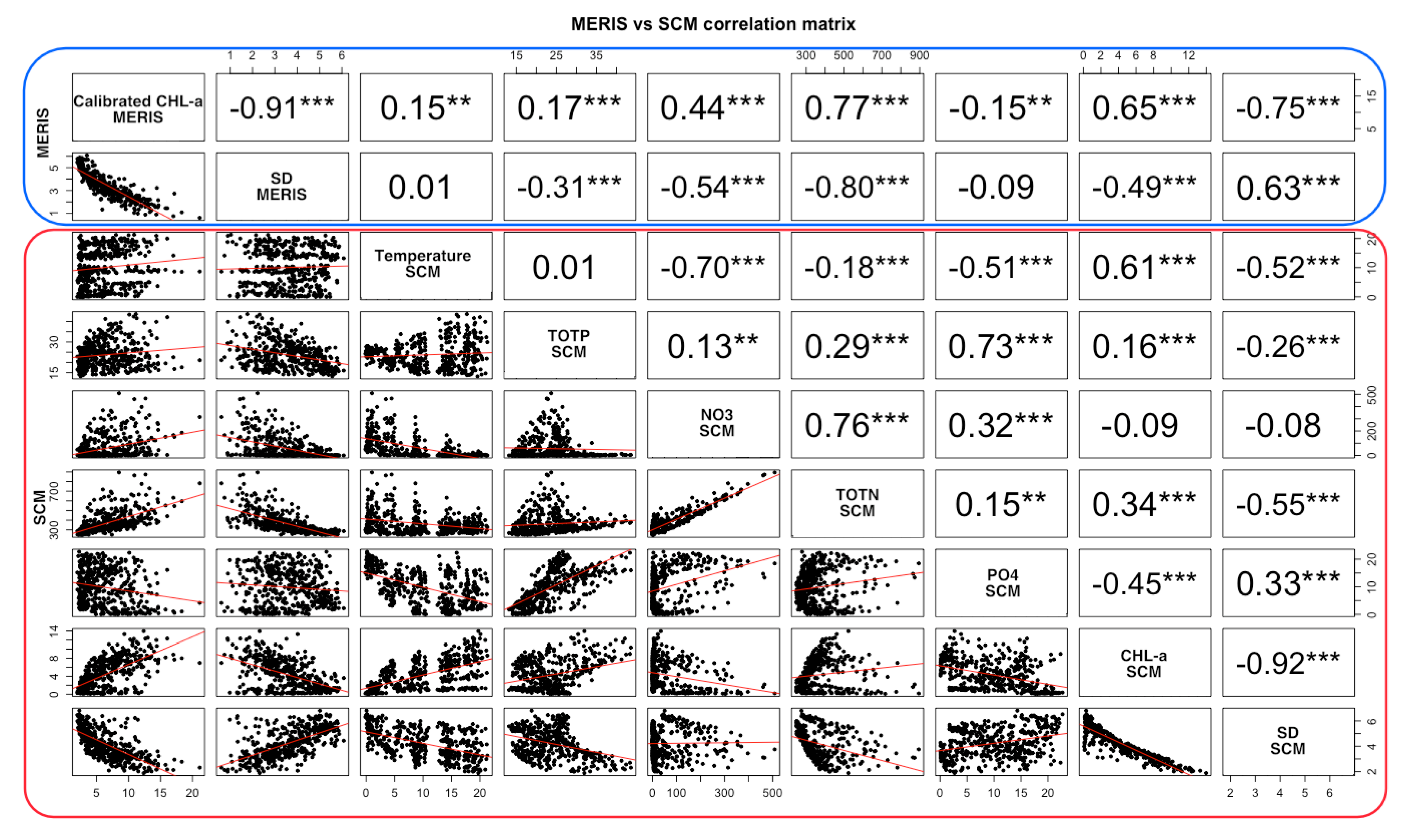
3.3. Comparison between MERIS and SCM

The correlations matrix between calibrated CHL-a and SD derived from MERIS and the physico-biogeochemical parameters computed by the SCM (i.e., water Temp, TOTP, NO₃, TOTN, PO4, CHL-a and SD) is shown in Figure 8. The Spearman’s rank correlation coefficient (ρ) computed in the matrix indicates the degree of association between variables and parameters listed above. There was a very strong inverse correlation (ρ = −0.91), between MERIS-derived CHL-a and MERIS- derived SD. MERIS CHL-a correlates only modestly with NO3 (ρ = 0.44, p < 0.001), but there is a strong correlation with CHL-a parameterized in the SCM with ρ = 0.65; p < 0.001, and a strong inverse correlation with SD SCM (−0.75, p < 0.001).

SD derived from MERIS correlated only modestly with NO3 (ρ = −0.54, p < 0.001), CHL-a SCM (ρ = −0.49, p < 0.001) and with SD SCM (ρ = 0.63, p < 0.001). However, strong correlations were observed between SD MERIS and modelled total nitrogen from the SCM (ρ= −0.80), as well as (calibrated) CHL-a derived from MERIS and modelled total nitrogen (TOTN SCM, ρ = 0.77, p < 0.001) which suggests strong relationships between these estimates derived from these two completely independent methods.

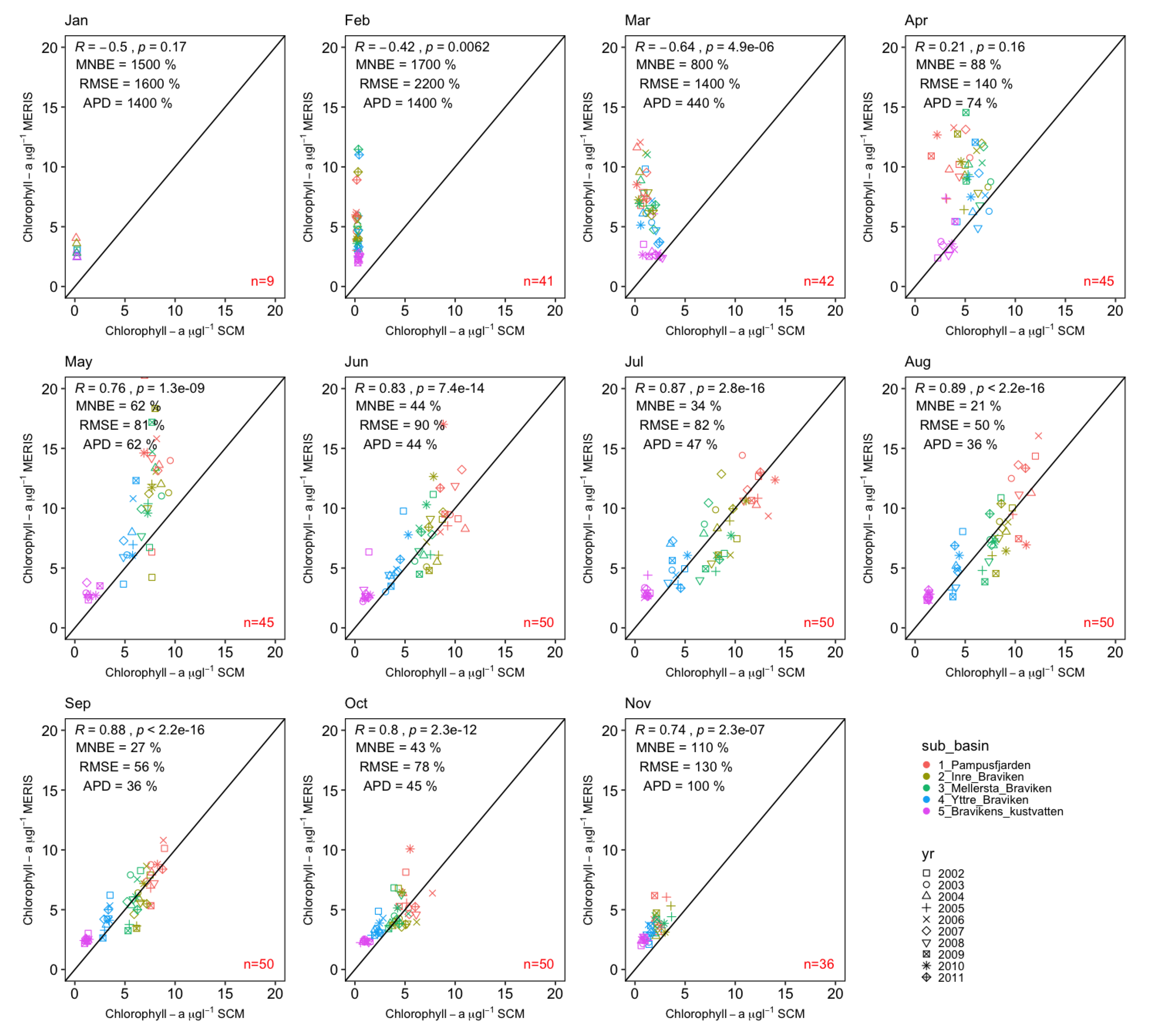
3.4. Evaluation of CHL-a Derived from MERIS versus CHL-a Derived from the SCM

The calibrated CHL-a derived from MERIS was plotted against CHL-a derived from the SCM (Figure 9). Each month was represented in an individual plot, each year was marked by a unique symbol, highlighting scatter points of a certain type that cluster together, suggesting yearly variability and internal coastal-open sea gradient through the five basins in Bråviken (coloured points). Figure 9 indicates a substantial overestimation of CHL-a by MERIS even after calibration for January (1500% MNB; 1600% RMSE; 1400% APD), February (1700% MNB; 2200% RSMSE; 1400% APD), March (800% MNB; 1400% RMSE; 440%APD), April (88%; 140%; 74%). This is most likely linked to the low water-leaving radiance due to low sun angle and possible contribution of ice and snow reflectance in winter, making the retrieval of CHL-a even more difficult in such highly absorbing waters. The satellite data from winter (January–April) thus must be treated with caution as it has very high errors, indicating poor agreement with modelled data.

Further splitting of the dataset into different basins did not improve the correlations (presumably because of the relatively low variability within each individual basin), and thus the data set was separated into different months (Jan–Dec, Figure 9) and the errors as well as the correlation coefficient were derived on a monthly basis. This showed significantly improved errors and correlation between calibrated CHL-a derived from MERIS and CHL-a derived from the SCM for all months between June (44% MNB; 90% RMSE; 44% APD) and October (43% MNB; 78% RMSE; 45% APD). For these months the data points were well distributed around 1:1 line with an acceptable bias below 50% and absolute difference of 36%–44%. The ρ values were reported for each month (Figure 9) where the number of observations (n) and the statistics were noted on each monthly plot. The highest Spearman’s correlation coefficients were reported for summer and fall, with August showing a maximum ρ value of 0.89, indicating very strong correlations between modelled and remotely sensed CHL-a values.

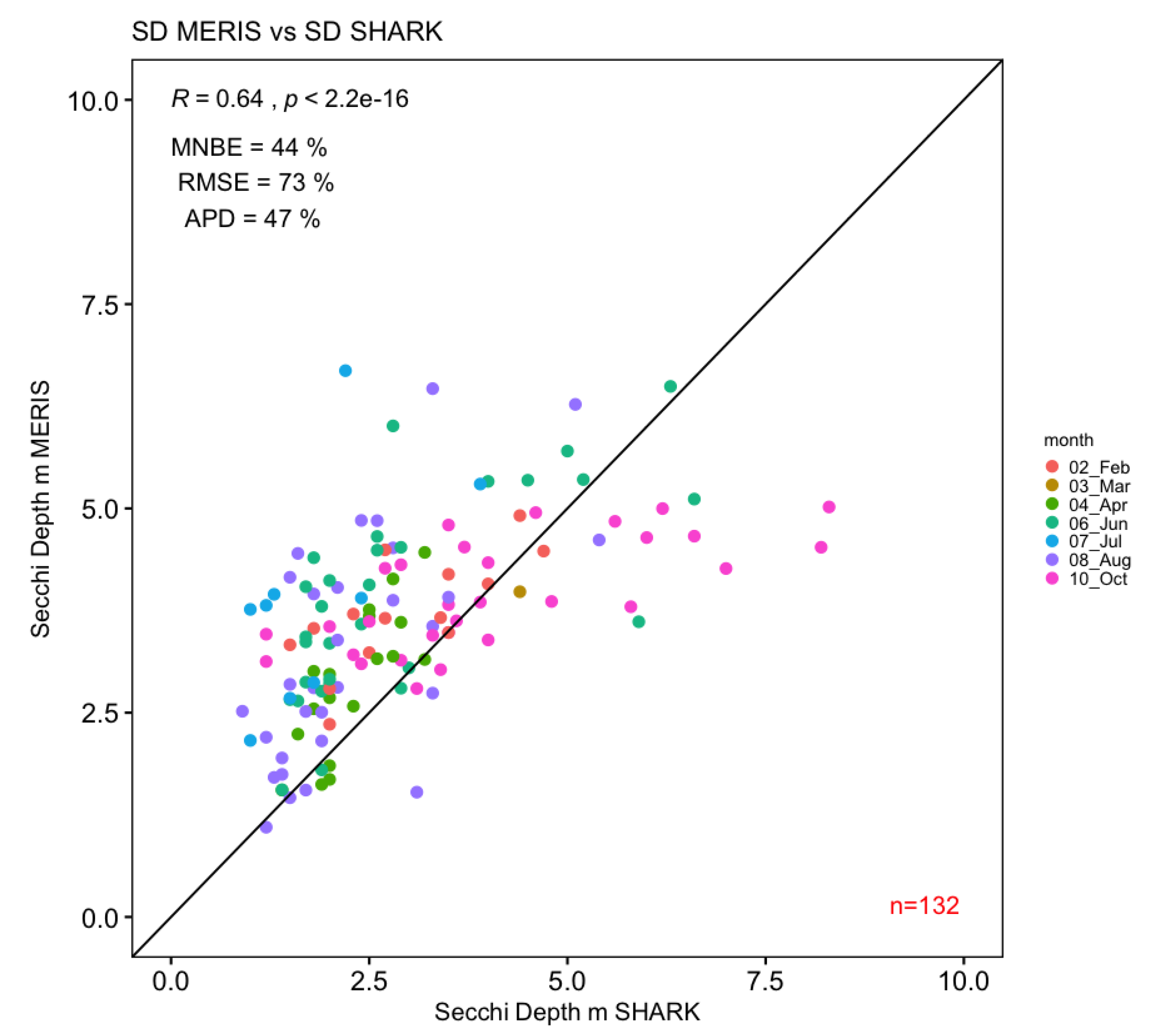
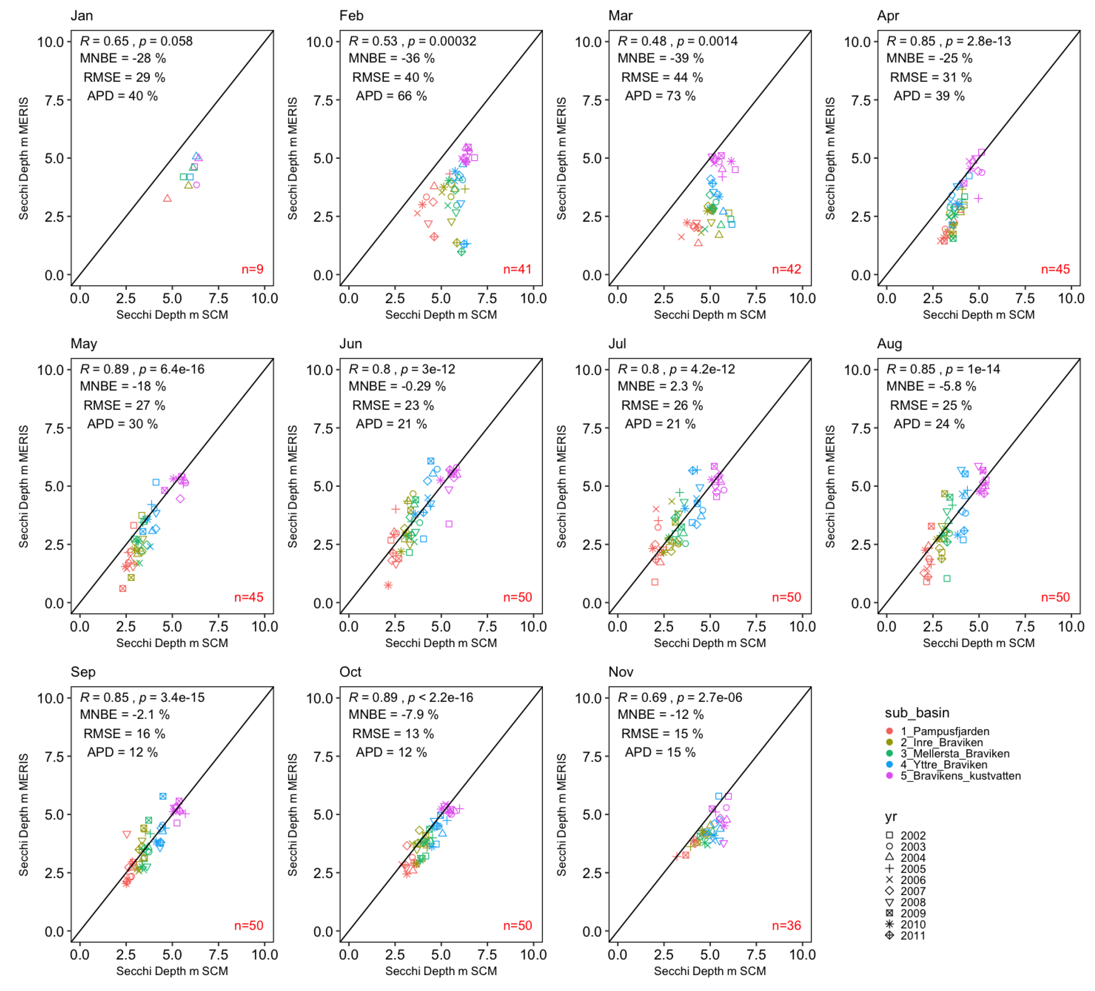
3.5. Evaluation of Secchi Depth Derived from MERIS versus Modelled Secchi Depth

A similar analysis was applied to Secchi depth derived from MERIS and modelled SD (SCM), (Figure 10), highlighting strong correlations through April–November with SD (MERIS) clearly underestimated in February and March. Observations in January were limited to only a few data points, nonetheless showing a reasonable underestimation of only −28% MNB and a relative error of 29% (RMSE) and 40% APD while there were no observations available at all from MERIS for December, presumably due to the low sun angles in winter and the effect of snow and ice reflectance.

SD (MERIS) was underestimated between February (−36% MNB; 40% RMSE; 66% APD) and April (−25% MNB; 31% RMSE; 39% APD), aggregating further around the 1:1 line from May (with −18% MNB; 27% RMSE; 30% APD) onwards and through to October showing the best statistical values (−8% MNB; 13%RMSE; 12% APD). The highest correlation coefficients were observed for May (−18% MNB; 27% RMSE; 30% APD) and October with identical ρ = 0.89. The split into different months indicated that the degree of association between SD MERIS and SD SCM had discrepancies in the first part of the year, significantly improving throughout the summer months through to December where no observations from MERIS were available for comparison. Overall, the results showed good agreement between measurements done by MERIS and the output of equivalent ecosystem state variables generated by SCM.

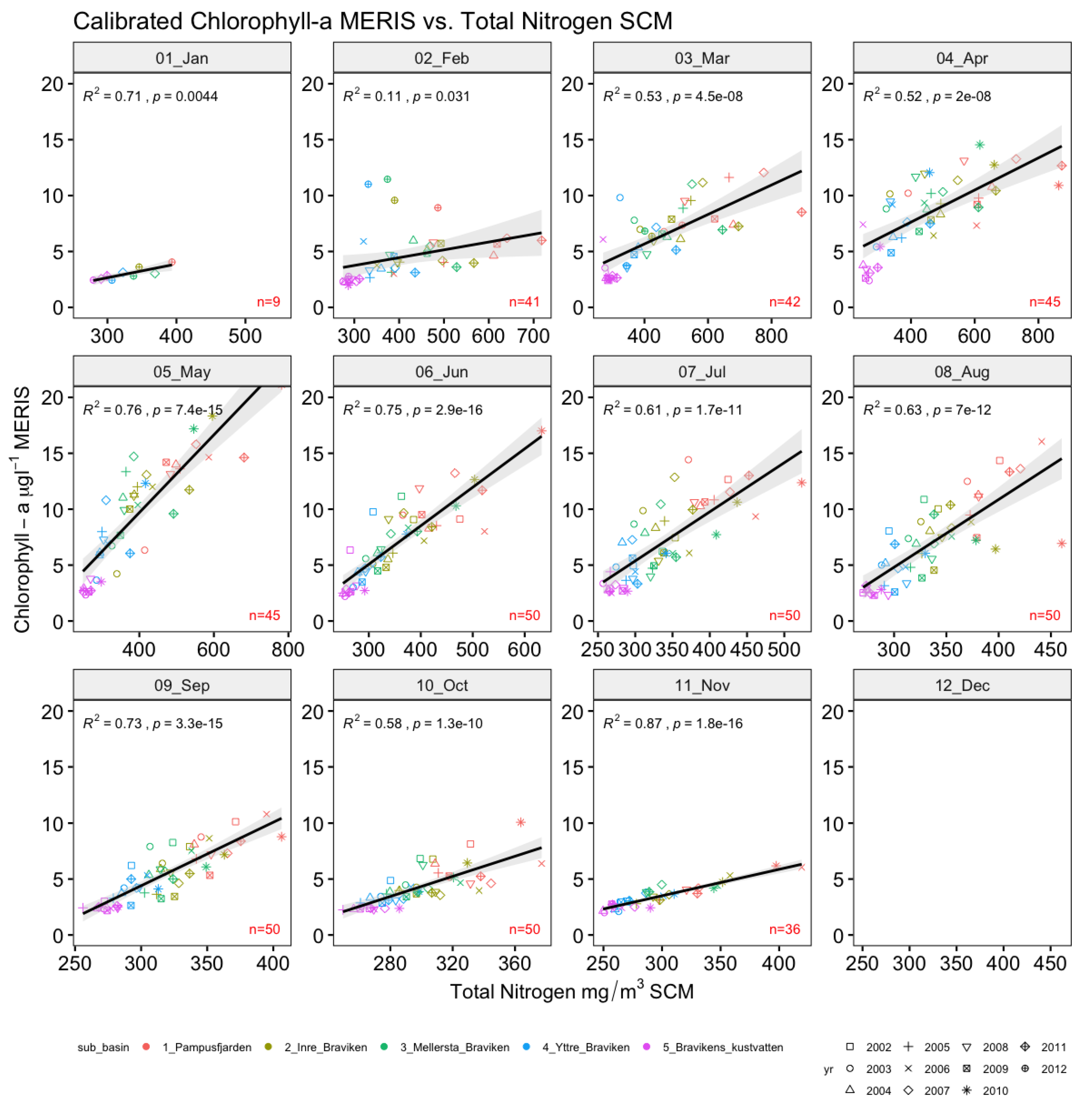
3.6. Relationship between Calibrated CHL-a (MERIS) and Modelled Total Nitrogen (SCM)

Calibrated CHL-a_MERIS was linearly regressed against concentrations of total N (TOTN) estimated in SCM (${\mathrm{R}}^2$ = 0.41, p < 0.001, all data, not shown) indicating a significant predictive power between the two sets of estimates. The distribution of points on scatter plot suggested a non-normal distribution with a cluster of data points aggregating at lower ranges of CHL (2.5–6 μgl⁻¹) and TOTN (less than 400 mg/m³). There was also a substantially stronger scatter at the higher ranges of values. Next, the datasets were split on a monthly basis and fitted with linear models (Figure 11). For January, the linear model fit yielded a coefficient of determination, R², of 0.71 (p < 0.001), although only based on a limited number of observations (n = 9). The strong correlation could be explained by a lower biological activity during this time of the year. In February, the outliers associated with year 2012 (Figure 11; 02_Feb) decreased R², to 0.11, indicating hardly any predictive power at all. These outliers may have been caused by the strong reflection from snow/ice cover as well error associated with retrieving CHL-a in the Nordic latitudes from satellite data due to low sun angles during winter period. For March and April, the linear fit produced coefficients of determination, R², of 0.53 (p < 0.001) and 0.52 (p < 0.001), respectively, and with a slightly increased slope. May scored the highest coefficient of determination: 0.76 (p < 0.001) for the later spring-summer period, indicating that TOTN can be predicted well in May from calibrated CHL-a (MERIS) with relatively high confidence. Similar strong relationships occurred in June with ${\mathrm{R}}^2$= 0.76 (p < 0.001) and started to decrease in July and August with ${\mathrm{R}}^2=$0.61 (p < 0.001) and 0.63 (p < 0.001), respectively, and with a better fit again in September, ${\mathrm{R}}^2$= 0.73 (p < 0.001), and lower again in October ${\mathrm{with}\mathrm{R}}^2=$ 0.58 (p < 0.001), and with the highest coefficient of determination of 0.87 in November, however with a lower number of observations (n = 36).

Another way of analysing and comparing the data from the different methods is by plotting time series of the MERIS, in situ and modelled CHL-a data to see how well each of them depict phytoplankton phenology [51]. Figure 12 shows the time series during the last HELCOM assessment period for inner Bråviken. Even though the MERIS data shows only the monthly means it is still able to depict the typical bimodal phytoplankton phenology with the highest CHL-a peak in spring followed and a somewhat lower CHL-a peak during the summer months. The monitoring data is too sparse to show a yearly trend, whilst the frequent modelling data also shows a bimodal phenology – albeit with a peak in spring and a second, higher peak during summer.

4. Discussion

4.1. Synergy between MERIS, In Situ and SCM Data

The synthesis approach applied here allows us to understand how different types of data and methods for assessing water quality in coastal zones agree with one another. For example, if there is good agreement (i.e., high correlation coefficient, ρ, low Mean Normalized Bias, Root-Mean Square Error and the average Absolute Percentage Difference). This implies that the methods can be used to complement one-another reliably. This synergistic approach allows us to choose between in situ measurements, satellite data or modelled data with the aim to get an improved estimate of the water quality status during the assessment period. Horizontal transects of CHL-a and SD derived directly from remote sensing reflectance data, provide additional information on the temporal variability of water quality between pre-defined monitoring stations (i.e., GB11, GB20, GB22 and GB16). The retrieval of CHL-a (calibrated using lake algorithm) and SD from MERIS showed a good agreement with in situ data (41% MNB; 96% RMSE; 63% APD and 44%; 73% and 47%, respectively) even though the discrepancies were higher compared to FUB performance in Himmerfjården area (27% MNB) from the dedicated MERIS validation campaigns in 2008–2010 [36]. These errors are expected considering the optically complex nature of Bråviken (high run-off/low salinity and CDOM in the inner part and higher salinity and open sea influence at the outer part). The errors associated with CHL-a retrieval were substantially reduced after applying the calibration algorithm (Figure 2), which gives additional confidence to the usability of MERIS data in coastal basins. Calibrated CHL-a values can be further used to substitute missing in situ data in-between SHARKweb stations as well as for the months and years when ship-based sampling did not take place. Similarly, calibrated CHL-a may support the validation of SCM performance for the time-frame or water body where in situ data are not available.

In the case of CHL-a measurements, in situ approaches are rather costly and time-consuming—resulting in a limited number of observations performed within the evaluated period (2002–2012) and observations only covering the summer months (June–August) of three years (2009–2011) out of a 10-year time-series in Bråviken (Figure 2 and Figure 3). Consistent in situ measurements were only performed in August throughout the entire time-series and there is no surface CHL-a data from ship monitoring available for the periods January-May and September-November, which leaves most of the months unmonitored. MERIS, however, delivered frequent data throughout most of the year apart from December and January (due to the low sun angles and low water-leaving reflectance in mid-winter). Figure 3 illustrates the relevance and applicability of MERIS over coastal waters to improve our understanding of the variability and distribution of CHL-a concentrations along the Bråviken gradient. The L3 MERIS data also can help to improve modelling of the gradient from the inner bay out to the open sea, and to validate model simulations of patchy water constituents, such as CHL-a during phytoplankton blooms. In situ Secchi depth data had an improved temporal coverage compared to CHL-a (Figure 5, Figure 6 and Figure 7), whilst the model can also provide data with good temporal coverage that is not feasible by remote sensing or monitoring efforts. The satellite only measures the top layers (to just below the Secchi depth) but with relatively high spatial resolution (300 m). The in situ data adds a vertical component, although with limited spatio-temporal resolution. The modelled data have improved temporal and spatial resolution (covering all Swedish coastal areas, and provides spatial information in tens of kilometres) as well as the highest temporal resolution (10 min) and provides also a good vertical resolution (0.5–4 m) akin to in situ measurements. The simultaneous use of additional data-sets can thus be used to fill in gaps found in the in situ data archive. This can significantly increase the spatial and temporal coverage of the coastal zone, while also highlighting discrepancies between the datasets and thus highlighting potential knowledge gaps.

4.2. Potential Advantages and Challenges for Monitoring Water Quality

The presented study demonstrates that the requirements set by the EU WFD [17] and the Marine Strategy Framework Directive (MSFD) [52] in terms of ‘good ecological/environmental status’ can only be assessed adequately by combining various approaches, spanning from conventional monitoring by ship, to observations performed by ocean colour sensors from Space [20,36], and to data modelled by hydrological and oceanographic biogeochemical models [45,46]. However, extensive validation with in situ data is required in order to assure reliable quality of ocean colour and modelling data. Validation also allows for testing and development of new remote sensing algorithms and model parameterization.

The study also highlights that sometimes novel steps have to be taken in order to improve currently available, state-of-the-art methods. Although MERIS was partially designed to improve coastal remote sensing, it still is known to have problems in discerning CHL-a in highly absorbing waters [36,41]. The calibration algorithm developed for Swedish Lakes (based on extensive in situ datasets) allowed to adjust CHL-a values also in Bråviken bay, an optically-complex waterbody with a rather large drainage area. Due to its elongated shape Bråviken acts as a transition zone between freshwater (high in phosphorus, nitrogen and organic matter) and the brackish waters of the Baltic proper which are nitrogen limited. The high CHL-a concentrations derived from MERIS in the innermost bay (i.e., Pampusfjärden) which were derived from MERIS before calibration can be explained by the presence of highly absorbing humic substance brought downstream via the Motala river. The FUB neural-network processor has the tendency to interpret high concentrations of coloured dissolved organic matter (CDOM) as high CHL-a concentrations (Figure 2, Figure 3 and Figure 4). This is mostly due to the fact that the FUB-processor was only trained for CDOM values up to 1 m⁻¹ which is not sufficient for inner coastal waters in the Baltic proper [33,35,36].

In a recent validation campaign during April 2018 dedicated to Sentinel-3 OLCI validation [50] observed waters in the Bråviken bay of yellow-brown colour throughout the inner basins (Pampusfjärden, Inner Bråviken and Mid-Bråviken) with very high CDOM concentrations of up to 13 m⁻¹ in Pampusfjärden. This supports the hypothesis that the FUB-processor cannot differentiate well between CHL-a and CDOM absorption, due to the optical dominance of CDOM absorption in inner bay. The same has been observed in other Baltic Sea coastal areas and in humic lakes. The calibration algorithm we applied derived from Swedish lakes [41] allowed to account for the discrepancy and to adjust the CHL-a values derived from MERIS so that the measurements corresponded well with the observed in situ measurements from the monitoring program (Figure 2). The algorithm can be applied to other waterbodies along the coast of the NW Baltic proper with similar coastal gradient dominated by CDOM, and will presumably perform likewise.

Previous research has shown that Bråviken has a relatively large coastal influence when compared to other areas in the NW Baltic proper [25,53]. Bråviken was chosen as a study site as it represents an optically-complex waterbody with both a strong inflow of freshwater dominated by CDOM in the most inner part (Pampusfjärden) and the brackish waters from the open Baltic Sea (Outer Bråviken). Applicability of the calibration algorithm in such diverse waterbody suggests a potentially better performance in less complex areas of the coastal zone as well as in the open Baltic Sea. The approach needs to be further tested in other areas of the Baltic Sea, e.g., the Gulf of Bothnia with an even more explicit CDOM dominance, or the coastal waters and bays in southern and eastern Baltic proper as well as the Gulf of Finland with a strong influence of suspended particulate matter [50,54,55,56,57,58,59].

Research has shown that the SD can be derived reliably from remote sensing data, which is promising as SD is an important water quality variable for Baltic Sea management [1,13,14,15,60,61]. This is why SD was chosen, along with CHL-a, as key optical properties in this study. Figure 6 demonstrated a similar pattern for the SD in situ measurements as for CHL-a Figure 3, although with a more frequent observations throughout the entire time-series. This may be explained by the fact that in situ SD measurements are much easier to perform—given there is no ice-cover. SD measurements can be done in a very short period of time, providing a quick and reliable measure of water transparency. Additionally, the method does not require specialized lab equipment and training, which is necessary for CHL-a measurements [62] and therefore is more cost-effective. Figure 6 shows that in situ Secchi depth measurements are even available for December almost through the entire time-series (apart from 2010 and 2012), where MERIS data were completely absent in December and January because of the too low sun angle at these high latitudes, and the interference of snow and ice cover. Norrköping is an industrial city with a harbour and thus the fairways are kept open for shipping throughout the winter, allowing for Secchi measurements to be taken also during seasons with ice-cover. Figure 3 and Figure 6 highlights how two sets of independent approaches in oceanography (remote sensing vs. in situ data) in one geographic area can complement each other by filling in observational gaps. The strong inverse correlation between MERIS-derived CHL-a and MERIS- derived SD (ρ = −0.91) was similar as found for bio-optical studies in the Baltic proper (Figure 8). Harvey et al. [14], e.g., also found a very strong inverse correlation (r = −0.80) for LN(SD) vs. LN(CHL-a) for the Baltic proper- supporting the argument that SD derived from Space is a good proxy for phytoplankton biomass and thus can be used for eutrophication studies as suggested by HELCOM [14].

However, the correlations measured in situ by Harvey et al. [14] between SD and CHL-a were only modest for the Skagerrak (r = -0.44) and rather low for the Bothnian Sea (r = −0.25). So, these relationships must be regarded as rather basin-specific for the Baltic proper and thus may not be blindly transferred to all Baltic Sea basins. Harvey et al. [14] proposed commonality analysis of multiple regression analysis for the three different Baltic Sea basins (Baltic proper, Skagerrak and the Gulf of Bothnia) to model Secchi depth, and thus water transparency from the three main optical constituents CHL-a, CDOM and SPM (TSM/turbidity). They then used these regression models for the assessment of the eutrophication status and the Good/Moderate thresholds as defined by the EU Water Framework and Marine Strategy Directives [17,52]. Theoretically, this approach could also be applied in remote sensing as these are the three main optical variables that can be derived from remote sensing data.

Another application for remotely-sensed SD in oceanographic research is to directly use the respective variable derived from remote sensing data as an input into biogeochemical or eutrophication models, or to the SCM presented in this study (see equation 4). SD is an important ecosystem state variable and can also serve as a proxy for the under-water light conditions [13], and thus representing one of the main drivers of productivity. Remote sensing data could significantly improve the parametrization of SD in oceanographic models, and is likely to improve the uncertainties in SD as an input variable due to the improved sampling frequency. Another input for oceanographic models that can be derived from remote sensing data with its improved spatial resolution is CDOM, which, e.g., in the SCM is generated indirectly from DON, but can be derived directly from the absorption at 440 nm, which in turn is derived from remote sensing reflectance. This is especially timely, since the Case-2 Regional CoastColour Processor [63] applied to Sentinel-3 OLCI data is now able to reliably retrieve a proxy for CDOM with low bias and relative error (i.e., 7.7% MNB and 56% RMSE) in Himmerfjärden [26]. The current processor can also process MERIS data and thus could be used for the reprocessing of 2002–2012 archive to get a more reliable estimate of CDOM. It must also be noted that the SCM assumes CDOM to be a conservative tracer, which is not quite the case as CDOM is both broken down by bacteria as well as photobleaching [34,64], and its distribution curve indicates non-conservative distribution [16].

Optical variables can be sensed remotely by ocean colour satellites, which then can be used to evaluate modelled data if the satellite data have been validated and quality-assured. Bråviken was chosen here as a study site because it had shown interesting gradients of optical parameters on existing satellite data [25,53] and because there was also modelled data available which showed to perform well in the area of investigations (Section 2.4). Merging the MERIS FUB time-series with corresponding datasets derived from the SCM allowed to investigate relationships between equivalent variables such as calibrated CHL-a derived from MERIS and modelled CHL-a, as well as SD derived from MERIS data and modelled SD, and to investigate if any relationship to other modelled physico-biogeochemical parameters such as nutrients could be established. The correlation matrix (Figure 8) allowed to identify strong relationships, e.g., between calibrated CHL-a derived from MERIS and modelled total nitrogen with correlations coefficient of up to 0.77 for the entire period between 2002 and 2012. The agreement between the data sets is rather high considering that the time-series includes different years, months (that are expected to be highly variable due to seasonality) as well as including five different waterbodies along the strong optical gradient in Bråviken.

The main strength of ocean colour data lies in its good spatial and temporal resolution compared to in situ water quality measurements in the coastal zone (as here demonstrated for CHL-a and SD measurements; Figure 3 and Figure 6). The improved temporal resolution may help to reduce the uncertainties in monthly and yearly estimates of water quality/or nutrient loads in the coastal zone. Uncertainties in nutrient load estimates in hydrological models are usually determined by the combined uncertainties in discharge and nutrient loading estimates [65,66,67]. The majority of rivers in Sweden are well monitored for discharge, but large uncertainty may arise because of the monthly (or even less frequent) in situ monitoring of nutrients [67,68] and other water quality parameters. Based on an investigation in 12 Swedish rivers draining into the Baltic Sea, Westerberg et al. [67] found that discharge itself only explained a relatively small proportion of the uncertainties (±7–14%) in yearly nutrient loads. However, the main uncertainties in estimating loading seemed to arise mostly from infrequent nutrient measurements. The results presented in this study indicate that remote sensing may help to reduce the measurement uncertainties as the sampling is much more frequent, allowing for better estimates of water quality information. Besides that, the remote sensing method derives CHL-a directly from the remote sensing reflectance data and not indirectly from nutrient loading, and thus is not dependent on nutrient estimates in order to generate reliable CHL-a concentrations; besides this SD is derived directly and very reliably from remote sensing reflectance data using simple band ratios [61,69]. MERIS data may also provide the tools to improve the predictive power of oceanographic models [13].

One of the aims of the study was to identify if any relationship between the water quality variables derived from ocean colour data can be used as a predictor or a proxy for nutrient concentrations (Figure 11). In order to support the implementation of goals set by EU Directives [17,52] and the periodic assessments done by HELCOM [4,5,14] it is crucial to have information on nutrient concentrations. Since, for example, nitrogen and phosphorus do not have an optical signal in the visible they cannot be directly detected from Space. Ocean colour remote sensing uses the visible part of the electromagnetic spectrum which allows for the detection of CHL-a concentrations and deriving Secchi depth from Space. Tett et al. [2] demonstrated a linear relationship between TOTN and CHL-a in Himmerfjärden bay with $R^2$= 0.64 (on a log-log scale), with log₁₀ (CHL-a) = 2.19 log₁₀TN—2.56 based on in situ measurements. A similar relationship was found in Bråviken between calibrated CHL-a derived from MERIS and modelled total nitrogen for the summer month subset (June, July, August); with almost the same coefficient of determination, $R^2$ = 0.65, n = 150, and a similar slope: log₁₀ (CHL-a) = 2.39 log₁₀ (TOTN) − 5.25. Also, the in-water relationship established by Tett et al. [2], showed a very robust relationship between SD and total nitrogen (in log-scale), with an $R^2$ of 0.89, confirming the robustness of SD as an indicator of nutrient status in the Baltic proper.

The regression analysis of CHL-a derived from MERIS and modelled TOTN showed (Figure 11) a strong linear relationship, with the highest coefficient of determination ($R^2$) of 0.76 for May during all years (2002–2012). In the Baltic Proper this is the time after the spring bloom and before the onset of the cyanobacteria summer bloom which usually starts in mid-June and lasts until end of August [62]. It is a time of year with relatively low biological activity, as most of the dissolved inorganic nitrogen has been used up during the spring bloom and most of the nitrogen thus would be contained in the particulate fraction, i.e., algal biomass. A similar variance is observed for June and September with slightly lower $R^2$ (0.75 and 0.73, respectively). Significantly lower $R^2$ were found for July and August (0.61 and 0.63, respectively). The highest coefficient of determination was identified for November with $R^2$ = 0.87 (n = 36), explaining 87% of the variability, and thus suggesting a very strong predictive potential. The large changes in the coefficient of determination may be explained by the seasonal succession patterns of the phytoplankton communities [70]. CHL-a derived from MERIS allows us to track the development of the spring bloom that normally occurs when light availability is not the main limiting factor anymore and dissolved inorganic nutrients are still plentiful in the water. The onset of the spring bloom usually happens between February-March in the southern Baltic Sea and during March-April in the Western Gotland Basin, with diatoms and dinoflagellates dominating the bloom. During this period none of the in situ CHL-a measurements were available from SHARKweb for any of the sub-basins in Bråviken. The early summer is characterized by a depletion of inorganic nutrients in the photic zone and a low phytoplankton biomass whilst the primary production is mostly sustained by regenerated nutrients. This is usually followed by a summer bloom during July/August, caused by large diazotrophic cyanobacteria – which are able to fix nitrogen directly from the air. The bloom is also maintained by high water temperature and stable weather conditions and is easily detected on satellite imagery which allows us to characterize their spatial extent [59,71]. However, the high proportion of cyanobacteria causes increased scatter (due to their internal gas vacuoles) which may affect CHL-a retrieval from satellite [72]. Later in the fall, when biomass declines approaching its annual minimum where conditions are characterized by low temperatures and light availability, limiting primary production. Nonetheless, there are certain cold-water phytoplankton groups such as diatoms that manage to survive at low concentrations in winter and thrive during early spring [70]. These seasonal changes in phytoplankton phenology as well as in run-off affect the inherent optical properties in the water, namely the absorption and scattering properties [72].

All in all, this study shows that the combined approach of methods with substantially increased spatial and temporal resolution is likely to provide new insights into ecosystem functioning and biological-physical interactions in highly productive coastal ecosystems. With the advances in ocean colour it is possible to map coastal water quality with unprecedented observational power and to analyse phytoplankton phenology as demonstrated in Figure 12, even when using monthly means. Many coastal waterbodies in Sweden are not monitored at all or at far too low frequency, as shown in Figure 3, Figure 6 and Figure 12. The low number of in situ observations in Bråviken bay (Figure 12) does not allow us to reliably analyse changes over time as, e.g., caused by climate change. Also, such infrequent in situ measurements are not able to depict phytoplankton phenology correctly and this cannot be used as a tool to adequately assess changes in phenology. Having said that, there are also more frequent coastal monitoring programs, as for example in Himmerfärden bay, where both satellite data and in situ data can depict phytoplankton phenology as well as CHL-a anomalies [21].

Both the satellite data and the modelled data in the Bråviken study indicate a spring and a summer bloom (Figure 12). However, the modelled summer bloom shows higher CHL-a values than during spring, and therefore does not quite correctly depict the phenology in the Baltic proper which usually consists of a large phytoplankton spring peak and a somewhat lower summer peak of filamentous cyanobacteria [21,73]. The results indicate that the model may need improved parametrization, e.g., by modulating the seasonal light attenuation as already discussed above.

The ESA MERIS mission (2002–2012) combined with the succeeding Sentinel-3 OLCI mission (operational since 2016 and planned up to 2030) can provide reliable, complementary synoptic water quality information, with increased frequency and with considerably improved spatial coverage when compared to the conventional, ship-based monitoring program. The long-term perspective of the combined MERIS and S3 missions will allow for improved monitoring and eutrophication assessment, providing reliable and frequent data and thus allowing us to characterise the measurements uncertainties accurately.

5. Conclusions

This study demonstrated how different means of observations can be used together with modelled data to better understand the state of a coastal ecosystem and help to better implement the goals set by the EU WFD and MSF Directives and HELCOM, especially with regards to eutrophication management. The scarcity in spatial and temporal coverage of monitoring data were addressed here using a 10-year time-series of ocean colour remote sensing data captured by the ESA MERIS sensor. The strength of the satellite data lies in its good spatial resolution and coverage, as well as in its good temporal frequency (even when using monthly mean values). The MERIS time-series allowed to evaluate horizontal gradients of CHL-a concentrations and Secchi depth from inner Bråviken bay out to the open sea. These optical variables can be used as proxies for phytoplankton biomass (CHL-a) and water clarity (SD), and thus are indicative of eutrophication. There was a good agreement of (spatially and temporally binned) Secchi depth and CHL-a derived from Space, and the respective in situ measurements from the monitoring program. The results from the regression analysis even showed that besides CHL-a there is a very strong agreement between Secchi depth retrieved from MERIS data vs. total nitrogen derived from the Swedish Coastal zone Model. The results confirm previous research in the Baltic proper that showed a very strong link between Secchi depth and total nitrogen measured in situ, making Secchi depth a very robust indicator of nutrient status and water transparency in the Baltic proper. Thus, Secchi depth may (together with CHL-a) be regarded as a key ecosystem state variable that can be derived directly from remote sensing reflectance data. The low-cost and high-frequency satellite data can also be used for water quality assessment in those coastal water bodies where in situ observations are not available at all. As Sweden is committed to monitor all Swedish water bodies by binding international agreements, there is a direct need for implementing these methods in the national monitoring program, especially in the open sea where there is a lack of monitoring data. As the satellite method has shown to be reliable, more frequent and can sense almost all coastal water bodies it has also the potential to reduce uncertainties in monthly and yearly water quality estimates in Swedish coastal waters. Besides this, MERIS is able to correctly depict the bimodal phytoplankton phenology in the Baltic Sea, even in its coastal areas, with a CHL-a peak in spring (diatoms and dinoflagellates) as well as a second, somewhat lower summer peak (i.e., filamentous cyanobacteria).

As ocean colour satellite data has been available for several decades, and remotely sensed Secchi depth can be derived reliably in the Baltic Sea, multi-mission data from various ocean colour sensor can be combined and used for long-term assessment, e.g., to assess effects of climate change on ecosystem state, water transparency and phytoplankton phenology.

References

- Harvey, E.T.; Walve, J.; Andersson, A.; Karlson, B.; Kratzer, S. The Effect of Optical Properties on Secchi Depth and Implications for Eutrophication Management. Front. Mar. Sci. 2019, 5, 1–19. [Google Scholar] [CrossRef]
- Tett, P.; Gilpin, L.; Svendsen, H.; Erlandsson, C.P.; Larsson, U.; Kratzer, S.; Fouilland, E.; Janzen, C.; Lee, J.Y.; Grenz, C.; et al. Eutrophication and some European waters of restricted exchange. Cont. Shelf Res. 2003, 23, 1635–1671. [Google Scholar] [CrossRef] [Green Version]
- Nixon, S.W. Coastal marine eutrophication: A definition, social causes, and future concerns. Ophelia 1995, 41, 199–219. [Google Scholar] [CrossRef]
- HELCOM. Eutrophication in the Baltic Sea—An integrated thematic assessment of the effects of nutrient enrichment and eutrophication in the Baltic Sea region. In Baltic Sea Environment Proceedings 115B; Baltic Marine Environment Protection Commission – HELCOM: Helsinki, Finland, 2018. [Google Scholar]
- HELCOM. State of the Baltic Sea – Second HELCOM holistic assessment 2011-2016. In Baltic Sea Environment Proceedings 155; Baltic Marine Environment Protection Commission – HELCOM: Helsinki, Finland, 2018. [Google Scholar]
- Saaltink, R.; van der Velde, Y.; Dekker, S.C.; Lyon, S.W.; Dahlke, H.E. Societal, land cover and climatic controls on river nutrient flows into the Baltic Sea. J. Hydrol. Reg. Stud. 2014, 1, 44–56. [Google Scholar] [CrossRef] [Green Version]
- Golterman, H.L.; de Oude, N.T. Eutrophication of Lakes, Rivers and Coastal Seas BT—Water Pollution. In Water Pollution; Allard, B., Craun, G.F., de Oude, N.T., Falkenmark, M., Golterman, H.L., Lindstrom, T., Piver, W.T., Eds.; Springer: Berlin/Heidelberg, Germany, 1991; pp. 79–124. ISBN 978-3-540-46685-7. [Google Scholar]
- Boesch, D.F.; Hecky, R.; O’Melia, C.; Schindler, D.; Seitzinger, S. Eutrophication of Swedish Seas; Swedish Environmental Protection Agency Naturvårdsverket: Stockholm, Sweden, 2006; ISBN 9162055097.
- Boesch, D.; Carstensen, J.; Paerl, H.W.; Skjoldal, H.R.; Voss, M. Eutrophication of seas along Sweden’s West Coast. In Report no. 5898; Swedish Environmental Protection Agency: Stockholm, Sweden, 2008; 79p, ISBN 978-91-620-5898-2. [Google Scholar]
- Vahtera, E.; Conley, D.J.; Gustafsson, B.G.; Kuosa, H.; Pitkänen, H.; Savchuk, O.P.; Tamminen, T.; Viitasalo, M.; Voss, M.; Wasmund, N.; et al. Internal Ecosystem Feedbacks Enhance Nitrogen-fixing Cyanobacteria Blooms and Complicate Management in the Baltic Sea. Ambio 2007, 36, 186–194. [Google Scholar] [CrossRef]
- Voss, M.; Dippner, J.W.; Humborg, C.; Hürdler, J.; Korth, F.; Neumann, T.; Schernewski, G.; Venohr, M. History and scenarios of future development of Baltic Sea eutrophication. Estuar. Coast. Shelf Sci. 2011, 92, 307–322. [Google Scholar] [CrossRef]
- Österblom, H.; Hansson, S.; Larsson, U.; Hjerne, O.; Wulff, F.; Elmgren, R.; Folke, C. Human-induced trophic cascades and ecological regime shifts in the baltic sea. Ecosystems 2007, 10, 877–889. [Google Scholar] [CrossRef]
- Kratzer, S.; Therese Harvey, E.; Philipson, P. The use of ocean color remote sensing in integrated coastal zone management—A case study from Himmerfjärden, Sweden. Mar. Policy 2014, 43, 29–39. [Google Scholar] [CrossRef]
- HELCOM. The Baltic Sea Action Plan (BSAP). In Proceedings of the HELCOM Ministerial Meeting of the Helsinki Commission, Krakow, Poland, 15 November 2007. [Google Scholar]
- Kratzer, S.; Håkansson, B.; Sahlin, C. Assessing Secchi and photic zone depth in the Baltic Sea from satellite data. Ambio 2003, 32, 577–585. [Google Scholar] [CrossRef]
- Kratzer, S.; Tett, P. Using bio-optics to investigate the extent of coastal waters: A Swedish case study. Hydrobiologia 2009, 629, 169–186. [Google Scholar] [CrossRef]
- European Communities; Water Framework Directive (WFD). Directive 2000/60/EC of the European Parliament and of the Council of 23 October 2000 Establishing a Dramework for Community Action in the Field of Water Policy. Official Journal of the European Communities 2000, L327, 1–73. [Google Scholar]
- Naturvårdsverket. Naturvårdsverkets Författningssamling; NFS 2006:1; Naturvårdsverket: 2004; Swedish Environmental Protection Agency: Stockholm, Sweden, 2006. (In Swedish)
- Rantajärvi, E.; Olsonen, R.; Hällfors, S.; Leppänen, J.M.; Raateoja, M. Effect of sampling frequency on detection of natural variability in phytoplankton: Unattended high-frequency measurements on board ferries in the Baltic Sea. ICES J. Mar. Sci. 1998, 55, 697–704. [Google Scholar] [CrossRef]
- Harvey, T.; Kratzer, S.; Philipson, P. Satellite-based water quality monitoring for improved spatial and temporal retrieval of chlorophyll-a in coastal waters. Remote Sens. Environ. 2015, 158, 417–430. [Google Scholar] [CrossRef]
- Beltrán-Abaunza, J.M.; Kratzer, S.; Höglander, H. Using MERIS data to assess the spatial and temporal variability of phytoplankton in coastal areas. Int. J. Remote Sens. 2016, 38, 2004–2028. [Google Scholar] [CrossRef]
- Donnelly, C.; Dahné, J.; Strömqvist, J.; Arheimer, B. Modelling Tools: From Sweden to Pan-European Scales for European WFD Data Requirements. In Proceedings of the BALWOIS 4th International Conference (BALWOIS 2010), Ohrid, Republic of Macedonia, 25–29 May 2010; pp. 25–29. [Google Scholar]
- Platt, T.; White, G.N.; Zhai, L.; Sathyendranath, S.; Roy, S. The phenology of phytoplankton blooms: Ecosystem indicators from remote sensing. Ecol. Model. 2009, 220, 3057–3069. [Google Scholar] [CrossRef]
- Alikas, K.; Reinart, A. Validation of the MERIS products on large European lakes: Peipsi, Vänern and Vättern. Hydrobiologia 2008, 599, 161–168. [Google Scholar] [CrossRef]
- Kyryliuk, D. Total Suspended Matter Derived from MERIS Data as an Indicator of Coastal Processes in the Baltic Sea. Master’s Thesis, Stockholm University, Stockholm, Sweden, 2014. [Google Scholar]
- Kyryliuk, D.; Kratzer, S. Evaluation of Sentinel-3A OLCI products derived using the Case-2 Regional CoastColour Processor over the Baltic Sea. Sensors 2019, 16, 3609. [Google Scholar] [CrossRef] [PubMed]
- Westman, Y.; Pettersson, O.; Wingqvist, E. Arbete med SVAR version 2016, Svenskt Vattenarkiv - en databas vid SMHI; Swedish Meteorological and Hydrological Institute: Norrköping, Sweden, 2017. (In Swedish)
- Gullstrand, M.; Löwgren, M.; Castensson, R. Water issues in comprehensive municipal planning: A review of the Motala River Basin. J. Environ. Manag. 2003, 69, 239–247. [Google Scholar] [CrossRef]
- SMHI SVAR2012_2. Available online: https://www.smhi.se/data/hydrologi/sjoar-och-vattendrag/ladda-ner-data-fran-svenskt-vattenarkiv-1.20127 (accessed on 19 July 2019).
- Copernicus EU-DEM v1.1—Copernicus Land Monitoring Service. Available online: https://land.copernicus.eu/imagery-in-situ/eu-dem/eu-dem-v1.1/view (accessed on 19 July 2019).
- SMHI SHARKweb Database. Available online: https://sharkweb.smhi.se (accessed on 19 July 2019).
- SMHI Havsmiljödata-Marine Environmental Data | SMHI. Available online: https://www.smhi.se/data/oceanografi/havsmiljodata (accessed on 19 July 2019).
- Schroeder, T.; Schaale, M.; Fischer, J. Retrieval of atmospheric and oceanic properties from MERIS measurements: A new Case-2 water processor for BEAM. Int. J. Remote Sens. 2007, 28, 5627–5632. [Google Scholar] [CrossRef]
- Kowalczuk, P.; Stedmon, C.A.; Markager, S. Modeling absorption by CDOM in the Baltic Sea from season, salinity and chlorophyll. Mar. Chem. 2006, 101, 1–11. [Google Scholar] [CrossRef]
- Kratzer, S.; Vinterhav, C. Improvement of MERIS level 2 products in baltic sea coastal areas by applying the improved Contrast between Ocean and Land Processor (ICOL)—Data analysis and validation. Oceanologia 2010, 52, 211–236. [Google Scholar] [CrossRef]
- Beltrán-Abaunza, J.M.; Kratzer, S.; Brockmann, C. Evaluation of MERIS products from Baltic Sea coastal waters rich in CDOM. Ocean Sci. 2014, 10, 377–396. [Google Scholar] [CrossRef] [Green Version]
- Florén, K.; Philipson, P.; Strömbeck, N.; Nyström Sandman, A.; Isaeus, M.; Wijkmark, N. Satellite-Derived Secchi Depth for Improvement of Habitat Modelling in Coastal Areas; AquaBiota Report 2012-02; AquaBiota Water Research: Stockholm, Sweden, 2012; ISBN 978-91-85975-18-1. [Google Scholar]
- Farr, T.G.; Rosen, P.A.; Caro, E.; Crippen, R.; Duren, R.; Hensley, S.; Kobrick, M.; Paller, M.; Rodriguez, E.; Roth, L.; et al. The shuttle radar topography mission. Rev. Geophys. 2007, 45, RG2004. [Google Scholar] [CrossRef]
- ESA CCI Land Cover ATBD. Algorithm Theoretical Basis Document: Pre-Processing Year 3- 1.1. Available online: https://www.google.com.hk/url?sa=t&rct=j&q=&esrc=s&source=web&cd=1&ved=2ahUKEwjHp5CIirHkAhWC7GEKHUQmDE0QFjAAegQIABAC&url=http%3A%2F%2Fcci.esa.int%2Ffiledepot_download%2F253%2F288&usg=AOvVaw2EW4EEGJCQNw1lFzmPstQG (accessed on 20 July 2019).
- Brockmann, C.; Paperin, M.; Danne, O.; Ruescas, A. Multi-Sensor Cloud Screening and Validation: IdePix and PixBox. In Proceedings of the 2013 European Space Agency Living Planet Symposium, Edinburgh, UK, 9–13 September 2013. [Google Scholar]
- Philipson, P.; Kratzer, S.; Ben Mustapha, S.; Strömbeck, N.; Stelzer, K. Satellite-based water quality monitoring in Lake Vänern, Sweden. Int. J. Remote Sens. 2016, 37, 3938–3960. [Google Scholar] [CrossRef]
- Hommersom, A.; Kratzer, S.; Strömbeck, N.; Philipson, P. Characterisation of the Optical Properties of Lake Vänern, Sweden, for Improved Water Quality Mapping by Remote Sensing. In Proceedings of the Extended Abstract and Poster Presentation at Ocean Optics, Glasgow, UK, 8–12 October 2012. [Google Scholar]
- Arheimer, B.; Nilsson, J.; Lindström, G. Experimenting with coupled hydro-ecological models to explore measure plans and water quality goals in a semi-enclosed Swedish Bay. Water 2015, 7, 3906–3924. [Google Scholar] [CrossRef]
- Sahlberg, J.; Marmefelt, E.; Brandt, M.; Hjerdt, N.; Lundholm, K. HOME Vatten i Norra Östersjöns Vattendistrikt Integrerat Modellsystem för Vattenkvalitetsberäkningar; SMHI, Oceanografi Rapport Nr. 93; Swedish Meteorological and Hydrological Institute: Norrköping, Sweden, 2008. (In Swedish)
- Edman, M.; Eilola, K.; Almroth-Rosell, E.; Meier, H.E.M.; Wåhlström, I.; Arneborg, L. Nutrient Retention in the Swedish Coastal Zone. Front. Mar. Sci. 2018, 5, 1–22. [Google Scholar] [CrossRef]
- Almroth-Rosell, E.; Edman, M.; Eilola, K.; Markus Meier, H.E.; Sahlberg, J. Modelling nutrient retention in the coastal zone of an eutrophic sea. Biogeosciences 2016, 13, 5753–5769. [Google Scholar] [CrossRef] [Green Version]
- R software for statistical computing (version 3.6.0). 2019. Available online: https://cran.r-project.org (accessed on 20 July 2019).
- Cristina, S.; Goela, P.; Icely, J. Assessment of water-leaving reflectances of oceanic and coastal waters using MERIS satellite products off the southwest coast of Portugal. J. Coast. 2009, II, 1479–1483. [Google Scholar]
- Lee, Z.P.; Du, K.P.; Arnone, R. A model for the diffuse attenuation coefficient of downwelling irradiance. J. Geophys. Res. C Ocean. 2005, 110, 1–10. [Google Scholar] [CrossRef]
- Kratzer, S.; Kyryliuk, D.; Brockmann, C. Inorganic Suspended Matter as an indicator of terrestrial influence in Baltic Sea coastal areas—Algorithm development, validation and ecological relevance. 2019. in review. [Google Scholar]
- Kyryliuk, D. Baltic Sea from Space. The Use of Ocean Color Data to Improve our Understanding of Ecological Drivers Across the Baltic Sea basin—Algorithm Development, Validation and Ecological Applications. Ph.D. Thesis, Department of Ecology, Environment and Plant Sciences, Faculty of Science, Stockholm University, Stockholm, Sweden, 2019. [Google Scholar]
- European Communities; Marine Strategy Framework Directive (MSFD). Directive 2008/56/EC of the European Parliament and of the Council of 17 June 2008 Establishing a Framework for Community Action in the Field of Marine Environmental Policy. Official Journal of the European Union 2008, L164, 19–40. [Google Scholar]
- Vinterhav, C. Remote Sensing of Baltic Coastal Waters Using MERIS—A Comparison of Three Case-2 Water Processors. Master’s Thesis, Deapartment of Physical Geography, Stockholm University, Stockholm, Sweden, 2008. [Google Scholar]
- Bukanova, T.; Kopelevich, O.; Vazyulya, S.; Bubnova, E.; Sahling, I. Suspended matter distribution in the south-eastern Baltic Sea from satellite and in situ data. Int. J. Remote Sens. 2018, 39, 9317–9338. [Google Scholar] [CrossRef]
- Kyryliuk, D.; Kratzer, S. Summer Distribution of Total Suspended Matter Across the Baltic Sea. Front. Mar. Sci. 2019, 5, 504. [Google Scholar] [CrossRef]
- Ohde, T.; Siegel, H.; Gerth, M. Validation of MERIS Level-2 products in the Baltic Sea, the Namibian coastal area and the Atlantic Ocean. Int. J. Remote Sens. 2007, 28, 609–624. [Google Scholar] [CrossRef]
- Raag, L.; Sipelgas, L.; Uiboupin, R. Analysis of natural background and dredging-induced changes in TSM concentration from MERIS images near commercial harbours in the Estonian coastal sea. Int. J. Remote Sens. 2014, 35, 6764–6780. [Google Scholar] [CrossRef]
- Toming, K.; Arst, H.; Paavel, B.; Laas, A.; Nõges, T. Spatial and temporal variations in coloured dissolved organic matter in large and shallow Estonian waterbodies. Boreal Environ. Res. 2009, 14, 959–970. [Google Scholar]
- Vaičiūtė, D.; Bresciani, M.; Bučas, M. Validation of MERIS bio-optical products with in situ data in the turbid Lithuanian Baltic Sea coastal waters. J. Appl. Remote Sens. 2012, 6, 63568. [Google Scholar] [CrossRef]
- Doron, M.; Babin, M.; Hembise, O.; Mangin, A.; Garnesson, P. Ocean transparency from space: Validation of algorithms estimating Secchi depth using MERIS, MODIS and SeaWiFS data. Remote Sens. Environ. 2011, 115, 2986–3001. [Google Scholar] [CrossRef]
- Alikas, K.; Kratzer, S. Improved retrieval of Secchi depth for optically-complex waters using remote sensing data. Ecol. Indic. 2017, 77, 218–227. [Google Scholar] [CrossRef]
- Schneider, B.; Dellwig, O.; Kuliński, K.; Omstedt, A.; Pollehne, F.; Rehder, G.; Savchuk, O. Biogeochemical cycles BT—Biological Oceanography of the Baltic Sea; Snoeijs-Leijonmalm, P., Schubert, H., Radziejewska, T., Eds.; Springer Netherlands: Dordrecht, The Netherlands, 2017; pp. 87–122. ISBN 978-94-007-0668-2. [Google Scholar]
- Brockmann, C.; Doerffer, R.; Peters, M.; Stelzer, K.; Embacher, S.; Ruescas, A. Evolution of the C2RCC neural network for Sentinel 2 and 3 for the retrieval of ocean colour products in normal and extreme optically complex waters. In Proceedings of the Living Planet Symposium, Prague, Czech Republic, 9–13 May 2016; Volume 740, pp. 9–13. [Google Scholar]
- Vodacek, A.; Blough, N.V.; DeGrandpre, M.D.; DeGrandpre, M.D.; Nelson, R.K. Seasonal variation of CDOM and DOC in the Middle Atlantic Bight: Terrestrial inputs and photooxidation. Limnology and Oceanography 1997, 42, 674–686. [Google Scholar] [CrossRef] [Green Version]
- Hägg, H.E.; Lyon, S.W.; Wällstedt, T.; Mörth, C.M.; Claremar, B.; Humborg, C. Future nutrient load scenarios for the Baltic Sea due to climate and lifestyle changes. Ambio 2014, 43, 337–351. [Google Scholar] [CrossRef] [PubMed]
- Lyon, S.W.; Meidani, R.; van der Velde, Y.; Dahlke, H.E.; Swaney, D.P.; Mörth, C.M.; Humborg, C. Seasonal and regional patterns in performance for a Baltic Sea Drainage Basin hydrologic model. J. Am. Water Resour. Assoc. 2015, 51, 550–566. [Google Scholar] [CrossRef]
- Westerberg, I.; Gustavsson, H.; Sonesten, L. Impact of discharge data uncertainty on nutrient load uncertainty. EGU Gen. Assem. Conf. Abstr. 2016, 18, 12039. [Google Scholar]
- Rönnback, P.; Sonesten, L.; Wallin, M. Ämnestransporter under Vårflöden i Ume älv och Kalix älv; Institutionen för vatten och miljö, Sveriges Lantbruksuniversitet, SLU: Uppsala, Sweden, 2009. (In Swedish) [Google Scholar]
- Kratzer, S.; Brockmann, C.; Moore, G. Using MERIS full resolution data to monitor coastal waters—A case study from Himmerfjarden, a fjord-like bay in the northwestern Baltic Sea. Remote Sens. Environ. 2008, 112, 2284–2300. [Google Scholar] [CrossRef]
- Andersson, A.; Tamminen, T.; Lehtinen, S.; Jürgens, K.; Labrenz, M.; Viitasalo, M. The pelagic food web. In Biological Oceanography of the Baltic Sea; Snoeijs-Leijonmalm, P., Schubert, H., Radziejewska, T., Eds.; Springer: Dordrecht, The Netherlands, 2017; pp. 281–332. ISBN 978-94-007-0668-2. [Google Scholar]
- Kahru, M.; Leppanen, J.M.; Rud, O. Cyanobacterial blooms cause heating of the sea surface. Mar. Ecol. Prog. Ser. 1993, 101, 1–8. [Google Scholar] [CrossRef]
- Kratzer, S.; Moore, G. Inherent Optical Properties of the Baltic Sea in Comparison to Other Seas and Oceans. Remote Sens. 2018, 10, 418. [Google Scholar] [CrossRef]
- Bernes, C. Change Beneath the Surface: An In-Depth Look at Sweden’s Marine Environment; Swedish Environmental Protection Agency: Stockholm, Sweden, 2005; ISBN 9162012460.