Article

A Robust Rule-Based Ensemble Framework Using Mean-Shift Segmentation for Hyperspectral Image Classification

by
Majid Shadman Roodposhti
1,*,
Arko Lucieer
1,
Asim Anees
2,3 and
Brett A. Bryan
4
1
Discipline of Geography and Spatial Sciences, School of Technology, Environments and Design, University of Tasmania, Churchill Ave, Hobart, TAS 7005, Australia
2
School of Engineering, University of Tasmania, Churchill Ave, Hobart, TAS 7005, Australia
3
Data Scientist Group, ProCan, Children’s Medical Research Institute, 214 Hawkesbury Road, Westmead, NSW 2145, Australia
4
Centre for Integrative Ecology, School of Life and Environmental Sciences, Deakin University, 221 Burwood Hwy, Burwood, VIC 3125, Australia
*
Author to whom correspondence should be addressed.
Remote Sens. 2019, 11(17), 2057; https://0-doi-org.brum.beds.ac.uk/10.3390/rs11172057
Submission received: 10 August 2019 / Revised: 26 August 2019 / Accepted: 29 August 2019 / Published: 1 September 2019
(This article belongs to the Special Issue Image Segmentation for Environmental Monitoring)

Abstract

:
This paper assesses the performance of DoTRules—a dictionary of trusted rules—as a supervised rule-based ensemble framework based on the mean-shift segmentation for hyperspectral image classification. The proposed ensemble framework consists of multiple rule sets with rules constructed based on different class frequencies and sequences of occurrences. Shannon entropy was derived for assessing the uncertainty of every rule and the subsequent filtering of unreliable rules. DoTRules is not only a transparent approach for image classification but also a tool to map rule uncertainty, where rule uncertainty assessment can be applied as an estimate of classification accuracy prior to image classification. In this research, the proposed image classification framework is implemented using three world reference hyperspectral image datasets. We found that the overall accuracy of classification using the proposed ensemble framework was superior to state-of-the-art ensemble algorithms, as well as two non-ensemble algorithms, at multiple training sample sizes. We believe DoTRules can be applied more generally to the classification of discrete data such as hyperspectral satellite imagery products.

Graphical Abstract

1. Introduction

Image classification is a vital tool for generating maps for environmental monitoring [1]. While for decades, multispectral imagery archives have been used to produce thematic maps, hyperspectral imagery is potentially a better option because of the higher spectral resolution. Hyperspectral images, which often contain more than 50 bands of continuous spectral information [2], can provide considerably more spatial and spectral information about the visible objects in their recorded field of view than multispectral imagery [3]. Because of the quality of information, hyperspectral images are widely used in applications such as precision agriculture [4], biotechnology [5], mineral exploration [6], and land-cover investigations [7]. These various types of applications have generated interest in hyperspectral image classification that has grown rapidly during the past two decades, with significant progress [8].
Up to now, many popular machine-learning algorithms have been applied in hyperspectral image classification. These include instance-based [9], regression [10], regularization [11], decision tree [12], probabilistic [13], reinforcement learning [14], dimensionality reduction [15], ensemble [16], Bayesian [17], maximum margin [18], evolutionary [19], clustering [9], association rule learning [20], artificial neural network [12,21,22] and deep learning [23] methods (see Figure 1). Regardless of the classification performance, many of these algorithms act as black-boxes, resulting in a poor recognition of the classification structure and robustness owing to the high-dimensionality of the data [24,25].
Recently, ensemble classification methods have received more attention from the machine learning community, resulting in their increased popularity in different applications such as hyperspectral image classification [26,27,28]. Nonetheless, as opposed to other black-box classification algorithms, rule-based ensembles have demonstrated the ability to inform the interpretation of classification schemes [29]. Rules are very general structures that offer an easily understandable and transparent way to find the most reliable class allocation [30]. The inferred logic of the model structure obtained by rule-based methods can be dissected, deciphered and applied out-of-the-box to new homogeneous classification problems. This is a major motivation, and it makes rule-based approaches more desirable compared with black-box approaches, even at the potential cost of a reduced classification accuracy [31]. This paper presents a simplified and novel rule-based ensemble framework based on the mean-shift and uncertainty assessment as a hyperspectral image classification tool, and we compare its performance against other state-of-the-art ensemble algorithms, where the mean-shift application is exclusive to the proposed framework. For the sake of simplicity throughout the paper, the proposed framework is referred to as DoTRules (Dictionary of Trusted Rules).
Here, we present DoTRules for hyperspectral image classification to provide a better and more transparent understanding of classification schemes, as well as accurate and robust classification performance. This adds to the growing literature of ensemble methods applied to the classification of hyperspectral data [32,33,34], especially those aimed at improving the performance of classification with acceptable clarity [35]. DoTRules is based on rules and uncertainty assessment. It was first introduced and applied to the calibration of land-use/cover change simulation models [36]. We assess the performance of the DoTRules algorithm as a novel rule-based classification framework modified to employ a bagging approach in order to boost accuracy. This accuracy boost is implemented by applying a thresholding assignment in order to extract trusted rules and then employing a novel voting approach to extract the class label recommended by the more trusted rules.
DoTRules extracts different subsets of training data from the full dataset, which can then be incorporated into boosting accuracy using a bagging approach designed to improve stability and accuracy. DoTRules has been found to perform well at modelling discrete data [37]. Since satellite imagery products inherently contain discrete digital numbers (DNs), DoTRules can work natively with them, quantifying the likelihood of belonging to a certain map class. It identifies classification rules and quantifies their frequencies so that some will be more influential than others. It also handles null values, which originate from unmatched rules between training and test samples. In addition, the uncertainty of every recognised classification rule is quantified using Shannon entropy. In simple terms, it scrutinises the uncertainty of each classification rule prior to assigning class labels based on their uncertainty value, so that the overall accuracy of classification can be improved. This not only results in boosting accuracy but also enables data analysts to spatially map every unique rule’s uncertainty. In terms of applying DoTRules, every pixel of the target hyperspectral dataset corresponds to one rule from each rule set, and, after quantifying uncertainty, only the most competitive one is selected among all of the corresponding rules for a target pixel. Thus, as opposed to many other methods, DoTRules is not a black-box method, as the attributes and characteristics of every single rule can be openly observed. In addition, by quantifying the uncertainty of every rule we can then anticipate their hit ratio. This provides a tool for the spatial segregation of more reliable/accurate classified boundaries from less reliable/accurate ones prior to image classification.
The main objectives of this study are to: (1) demonstrate DoTRules as an accurate and transparent rule-based ensemble framework for hyperspectral image classification; (2) map the uncertainty of every unique classification rule as an estimate of the rules’ hit ratio. This highlights the contribution of this paper, i.e., developing an accurate and transparent rule-based ensemble algorithm that provides a prior estimate of classification accuracy at the pixel level. Mapping the spatial distribution of classification accuracies is considered extremely beneficial for enhancing the capabilities of a classifier used as a land-use and land-cover map production tool based on satellite imagery [38,39]. Here, we describe the modified version of DoTRules for hyperspectral image classification, before demonstrating its application in three different study areas. We quantify the accuracy of DoTRules for hyperspectral image classification, and compare the results against some popular state-of-the-art ensemble approaches, i.e., extreme gradient boosting (XGBoost) [40,41], random forest (RF) [1,42,43,44,45], rotation forests (RoFs) [46,47,48,49], regularised random forest (RRF) [50,51], as well as two non-ensemble algorithms, namely, support vector machine (SVM) [52,53,54,55,56], and deep belief network (DBN) [57,58] as the classic deep learning method. Although SVM and DBN are not ensemble methods, they are included in our comparison because of their popularity, as they have been repeatedly used in recent hyperspectral image classification studies using Indian Pines, Salinas and Pavia University datasets. Finally, we discuss the advantages and disadvantages of the proposed approach for hyperspectral image classification.

2. Methods and Datasets
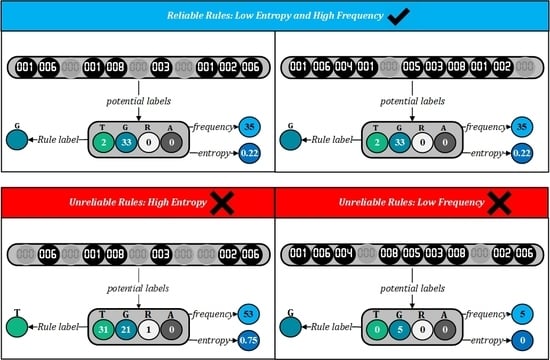
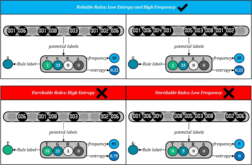
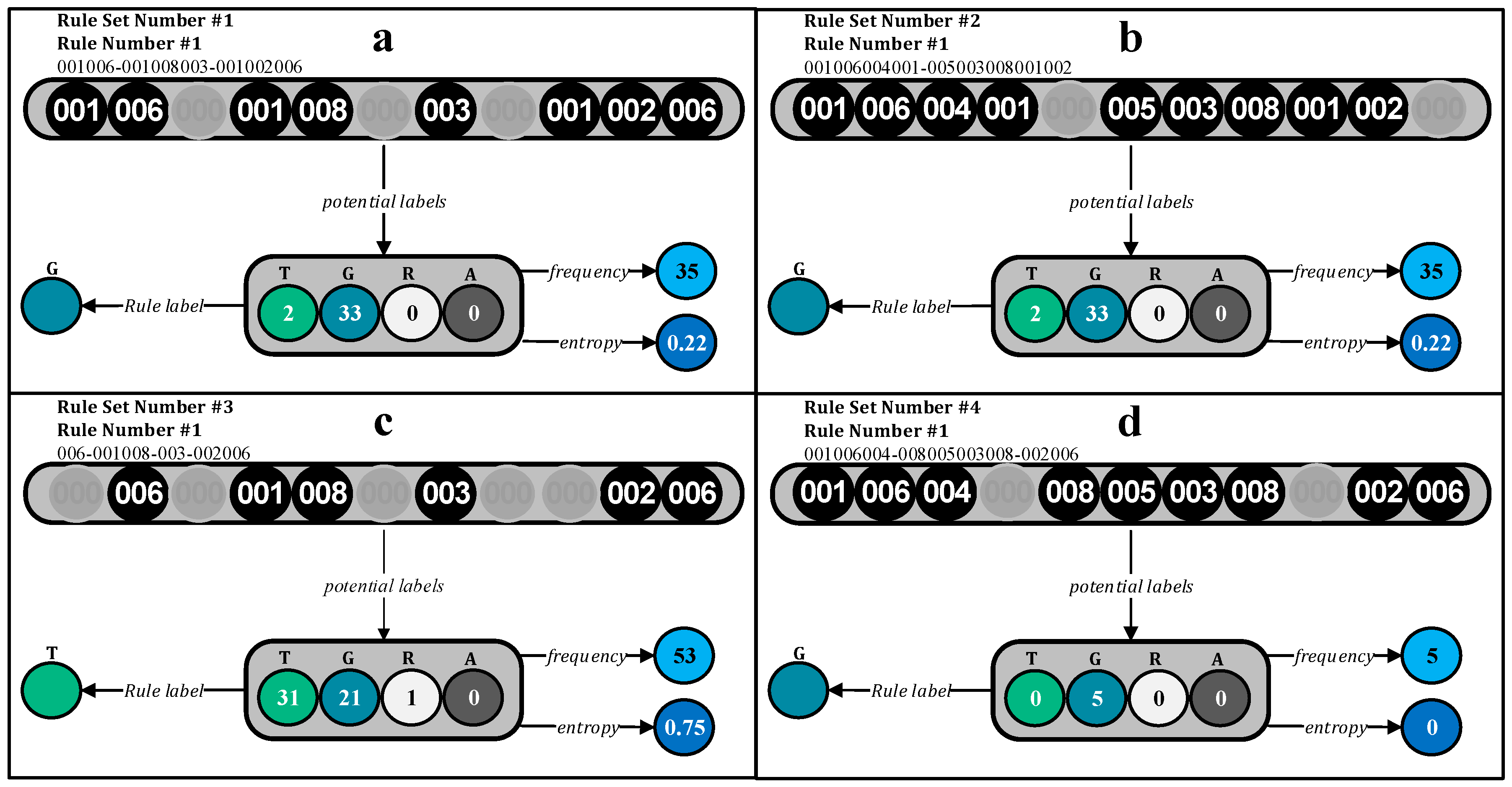
2.1. DoTRules

DoTRules is based on a dictionary of trusted rules. It is designed for prediction when a large amount of discrete data are involved. However, it may also be applied to continuous data after discretisation. This is similar to the RF [59,60] method insofar as rule sets are used to select the mode response (i.e., most frequent class label). However, instead of generating random trees, DoTRules operates by constructing many corresponding rules for every pixel (i.e., feature vector), which are derived from different rule sets. Each rule set is generated from a different combination of predictor variables in the ensemble run. For every unique rule, the most frequently occurring class label, which carries the highest probability of occurrence, is assigned [37,61]. However, as there are many rule sets, there may be many matching rules with defined class labels for a single data sample. To get the best (i.e., final) class label, a weighted majority filter (weighted mode) is applied on every available corresponding rule for a single data sample after the elimination of unreliable rules. The weighted majority filter puts more emphasis on those rules that are assembled by more components (i.e., matching variables) with less generalised class labels. The DoTRules procedure consists of the following steps implemented in R [62]:
STEP 1: Segmentation analysis
First, a data segmentation or segmentation analysis should be applied to each predictor variable J={j1,j2, …, jn} before classification, where J is a defined set of spectral bands/band combinations, but not necessarily every spectral band or a possible combination. These homogeneous digital numbers (DNs) of the hyperspectral satellite image are then converted to segments. This is intended to partition m observations of the original image into S segments for each j in J, in which each DN in each segment (ideally) shares some common trait. Although various types of segmentation or even clustering algorithms can benefit the proposed classification framework, here we applied a mean-shift segmentation algorithm [63]. The mean-shift algorithm [63,64] is a recursive algorithm that allows us to execute a nonparametric mode-based segmentation. This is performed by a data segmentation based on a kernel density estimate of the probability density function associated with the data-generating process. The main motivation for applying a mean-shift algorithm is the fact that it is model-free and does not assume any prior distribution shape for data segments. Furthermore, it is robust to outliers and does not require a pre-specification of the number of segments.
In its standard form, the mean-shift algorithm works as follows. We observe a set of DN values from x1,…,xm, for each spectral band J={j1,j2, …, jn}. We fix a kernel function ker f and a bandwidth parameter σ, and we apply the update rule:
x i = 1 m ker f ( x i x σ ) x i i = 1 m ker f ( x i x σ )
where σ is a bandwidth parameter. The fundamental parameter in mean-shift algorithms is the bandwidth σ, which determines the number of segments [65]. Furthermore, regions with less than some pixel-count C may be optionally eliminated. To account for different spatial and spectral variances it is practical to choose a kernel window of size σ = σs, σr with differing radii. σs is in the spatial domain, and σr is in the range domain. The statistics literature has developed various ways to estimate the bandwidth. One of them is the adaptive mean-shift where you let the bandwidth parameter vary for each data point. Here, the σ parameter is calculated using the kNN algorithm [66]. If xi,S is the k-nearest neighbour of xi, then the bandwidth is calculated as:
σ i = x i x i , S
Here, the aim of the segmentation analysis is to summarise the input data and then minimise the required number of rules for correctly classifying pixels to their corresponding class label. As more accurate segments will improve the classification results, it is beneficial to apply the segmentation analysis on spectral band compositions composed of less similar spectral bands (i.e., within multidimensional space). Thus, a pairwise dissimilarity measure dis(ji, jn) between spectral bands ji and jn, for 1 ≤ i, jn [67] can be applied to achieve more robust segments.
STEP 2: Formatting the data
In order to avoid mixing segment (S) values during the concatenation phase for the rule implementation in later steps, data segments should be formatted. Following the data segmentation, considering the maximum number of segments (S), the obtained data from step one should preferably be converted to two-digit (i.e., S < 100) or three-digit (i.e., 100 <= S < 1000) numbers, or more. This is a requirement prior to the rule implementation. Hence, if a maximum value of S is under 100, the data should be formatted in a two-digit format (e.g.,3 = 03, 26 = 26), while if the maximum value of S is =>100 and < 1000, then the data should be in a three-digit format (e.g., 3 = 003, 26 = 026), and so forth.
STEP 3: Splitting data into training and test samples
Both our training and test sets will be in a tabular form, consisting of a set of pixels I={i1,i2, .., im}. Each pixel i in I has a value xij for each predictor variable J. Simply, xij is the converted segment value of the sample i in I and j in J. Thus, for each predictor variable j, xij can adopt one of a fixed set of possible values ≤ S. Each pixel i has a corresponding class label li ∊ L={l1, l2, …, lh}, which are also discrete semantic attributes from the global set of class labels, such as corn, grass, oats, etc. It should be noted that to implement ensemble learners using DoTRules, we need to derive z sub-sets of our training dataset to construct different rule sets D containing individual classification rules d. This consists of all the available pixels in the primary training dataset but includes a different (random) combination of j in the feature vector.
STEP 4: Creating a rule set
For every zth sub-set of the training set, we will concatenate values of a pixel xij for every j in J to form a rule set D. The concatenation of two or more characters is the string formed by them in a series (i.e., the concatenation of 001, 020, and 200 is 001020200). Equation (3) illustrates the pixel values for the segmented predictor variables concatenated for each pixel (row) i, thereby creating a rule for each pixel in the corresponding subset of the training dataset.
D z = ( x 11 x 21 x m 1 ) | | ( x 12 x 22 x m 2 ) | | | | ( x 1 n x 2 n x m n ) = [ x 11 x 21 x m 1 x 12 x 22 x m 2 x 1 n x 2 n x m n ] = [ d 1 d 2 d m n ]
Note that following the concatenation and extraction of rules (Equation (3)), every rule within a specific rule set has maintained its single class label li ∊ L. We then aggregate duplicate rules where pixels have exactly the same values for all criteria, leaving an efficient new rule set of unique rules D′z. The frequency of occurrence of all potential class labels li ∊ L is then calculated for each unique rule d′ in D′z:
[ L 1 L 2 L v ] [ f ( l 1 ) f ( l 2 ) f ( l 3 ) f ( l h ) f ( l 1 ) f ( l 2 ) f ( l 2 ) f ( l h ) f ( l 1 ) f ( l 2 ) f ( l 3 ) f ( l h ) ]
where v is the number of unique rules in Dz. The class label from the set L with the highest frequency (i.e., the mode) is then assigned to each corresponding unique rule d′. The total number of rule sets D = [1, …, z] and the number of components in each rule set (i.e., the length of a rule) is user-defined. Although the classification accuracy may increase by using more rule sets, it will be at the expense of the computation cost. In terms of rule length, the accuracy of classification may not increase necessarily by the implementation of longer rules, where longer rules with more conditional components from the J set will model the training data too well (i.e., overfitting), resulting in less generalised responses for estimations of class labels, and vice versa (i.e., underfitting). Overall, as the quantity of matching pixels in the test dataset is inversely proportional to the length of rules, the longer rules with more components are more specific with fewer matches, while the shorter rules with fewer components are more general with many matches in the test dataset.
To ensure a more accurate estimation, the default value of z is set to 100 rule sets. Then, to avoid overfitting and underfitting issues, the number of predictor variables (j) used in every rule d within a specific rule set (length of rules within a considered rule set) is defined by a random function with a lower and upper bound defined by the user. This random function is called once, before creating every single rule set, to define the number and combination of components within that rule set. As the optimal combination of predictor variables is unknown, random band selection helps reduce the potential for the overfitting of the classifier. In this way, rules with various length will be implemented. The lower (min) and upper bound (max) for the length of rules (λ) in each rule set D = [1, …, z] is a positive natural number defined by:
λ { max ( λ ) n min ( λ ) > 0
where n is the number of selected predictor variables in J set. The number of rule sets, min and max values of λ can be further optimised using cross-validation.
STEP 5: Calculating and mapping rule entropy.
The aim of this step is to assess the uncertainty value of each rule. In information theory, entropy is the quantitative measure of system disorder, instability and uncertainty, and may be used to forecast the trend of a specified system. Entropy indicates the expected amount of information contained [68]. Here, the entropy value of every unique rule d′ from a rule set Dz is calculated based on the frequencies of each possible class label (Equation (4)) as:
e d = i = 1 h p l i log 2 p l i
where e d is the entropy of the unique rule d′ and Pli is the probability value of the class label liL. Here, h is the number of class labels in L. The general idea is that for a given rule, which may cover one or many pixels, the greater the probability of a class membership for a given class label, the less the uncertainty associated with that class. This provides a quantitative estimate of uncertainty for every single rule within different rule sets prior to assigning class labels. These estimates of uncertainty values can be applied to both the spatial mapping of rule uncertainty in classification, and to eliminating those unreliable rules with a high entropy from different subsets and/or rule sets before combining votes. The spatial distribution of uncertainty is quantified by mapping the entropy of each unique rule back to the corresponding pixels. These estimates of uncertainties are extremely beneficial and can be considered even prior to assigning class labels to pixels. Every time that DoTRules is applied to a training data subset, a class label of the highest frequency is allocated, and the entropy of that rule is calculated.
STEP 6: Eliminating unreliable rules within all rule sets.
After assessing the uncertainty of each individual rule, unreliable rules (i.e., rules with a high entropy) should be eliminated to improve the quality of the voting outcome, which directly affects the classification accuracy. Thus, every such rule d′ (in D′z), for which the e d is greater than the user-defined threshold, is eliminated. In our study, we specified that if e d is > 0.3 for a rule, and its corresponding pixel’s frequency is < α (to avoid randomness), then the rule is considered to be unreliable and is eliminated accordingly. α is calculated as follows, keeping the random chance for a resultant entropy value under 0.05%:
α = C e i l ( ln ( 0.05 ) ln ( 1 / h ) ) f o r h > 1
where h is the number of class labels.
STEP 7: Classifying the test dataset.
Above, we described the process of creating DoTRules and allocating the most likely class label for each rule based on the frequency. In the same way, class labels can now be assigned for the study area using another subset of the primary training dataset (i.e., implementing more rule sets). Every time a new rule set is implemented, the same procedure is followed to establish rules for the test dataset. We then match each test data rule with its equivalent training rules in the DoTRules using a many-to-one matching algorithm and allocate the most likely class label to each test data rule. This will be repeated every time that a weak learner is being implemented from every single rule set.
STEP 8: Handling null values
There is always a possibility of encountering null records in the test dataset while using DoTRules. In this situation, new pixels in the test dataset present combinations of states for criteria not encountered in the training data, which may increase the out of bag error. Handling null values is inevitable for maintaining the classification accuracy, where in the proposed ensemble framework using mean-shift it is a combined procedure. First, all rules are sorted based on their similarity, then every single null value is assigned to the class label of its closest (i.e., most similar) rule, based on the alphanumeric similarity of the constructed rules. However, the influence of these rules in combining votes is minimised as they are characterised by null entropy values.
STEP 9: Combining votes
In order to fulfil the classification procedure, this step is used to assign a final label to each pixel. To combine votes of each set of learners, we first remove all unreliable rules (with low or null entropy records) within every rule set using a thresholding approach. Afterwards, a mode filter is applied to the resultant class labels coming from sets of corresponding rules for each pixel. This mode function not only considers the frequency of class labels, but also considers the length of a rule as a weighted function. Since a rule is formed by concatenating n number of predictor variables (j), a rule that contains more predictor variables as components therefore has a higher weight in the mode function. Nonetheless, if none of the recognised reliable rules, for a certain pixel in the test dataset, is matched by any corresponding rule from the various training rule sets (derived from subsets of the training data), then the mode function will be applied to the corresponding labels of unreliable rules explained in STEP 8 with the same mode function.
STEP 10: Calculating and mapping the hit ratio
Calculating and mapping the hit ratio helps to visualise the spatial distribution of the classification error. Similar to the entropy value, which is calculated for every unique rule based on the frequencies of each possible class label, we map the hit ratio of every unique rule in our combined results back to the original pixels. DoTRules is rule-based, where every unique rule d′ from a rule set D′z corresponds to one or many pixels; thus, we can calculate the classification hit ratio of those rules using Equation (8):
A d = i = 1 h l i + / i = 1 h l i
Here, l i + is the sum of the correct classified labels.

2.2. Rule Uncertainty Threshold

In using DoTRules for the classification of hyperspectral imagery, the class label of a rule is also described by both its entropy value and the frequency of all potential class labels (Figure 2). Therefore, a rule can be considered reliable if its entropy is less than 0.3 bits, which is calculated at least for n potential class labels (frequency > α). However, it is important to note that among the reliable rules coming from the various rule sets for a certain pixel, those with a longer concatenated string (rule) will have more impact in combining final votes. This is mostly due to the fact that they are composed of more variables but meet the same uncertainty threshold, and hence can make more robust predictions. In other words, longer rules have fewer pixels with a specific class label, while shorter rules have more pixels belonging to multiple class labels. The fewer the pixels shared between different rules, the more accurate the classification results will be.
As the estimated entropy values for the distribution of response variables (class labels) with low frequencies are less reliable (Figure 2d) and may result from random chance, a second threshold is applied to the frequencies of potential labels. This will further improve the quality of the rule elimination process.

2.3. Comparing DoTRules with Other Methods
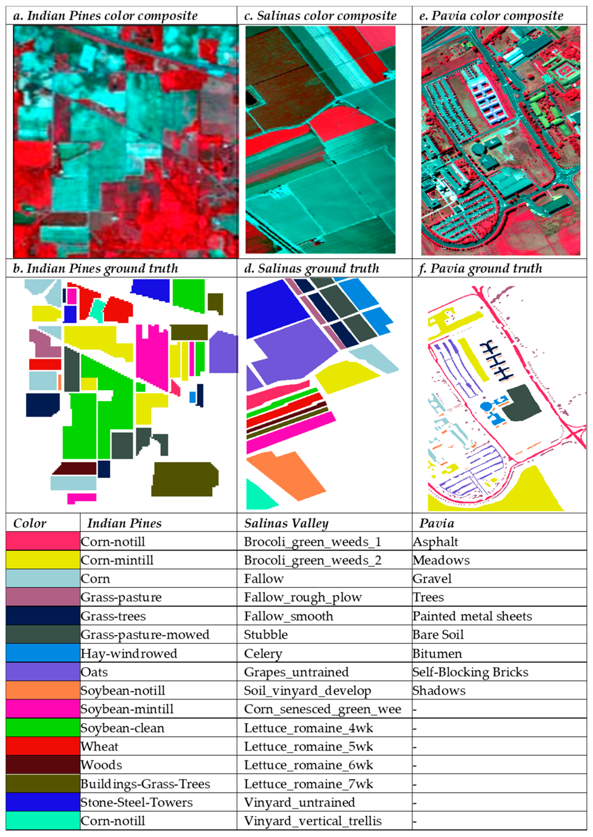
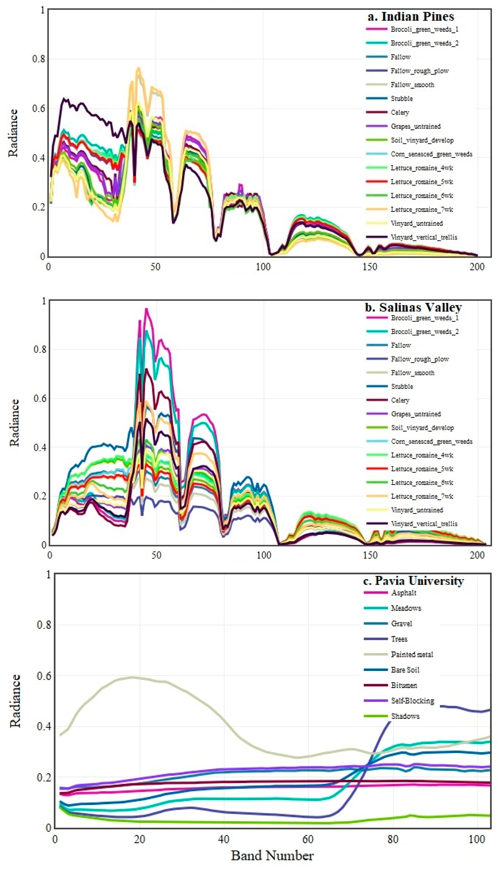
To measure and quantify DoTRules’ performance, we implemented different classification algorithms, including XGBoost, RF, RoF, RRF, SVM, and DBN on the same datasets. These six algorithms are among the most popular methods for hyperspectral image classification, and they belong to three different categories of machine-learning methods. The first four algorithms are state-of-the-art ensemble methods, while SVM is a maximum margin classifier and DBN is a deep learning method. Thus, these methods provide appropriate benchmarks for assessing the performance of the DoTRules. XGBoost is an algorithm that has recently been dominating applied machine learning [69], and RF, RoF and RRF were selected because of both their natural similarity to DoTRules and performance in hyperspectral data classification [1,42,43,44,45]. They are also computationally efficient and suitable for large training datasets with many variables and can solve multiclass classification problems [70]. Furthermore, SVM [9,18,71] and DBN [57,58] algorithms have demonstrated promising results in previous studies. We compared the overall accuracy (OA) and kappa coefficient (k) of DoTRules with these various algorithms for hyperspectral image classification, using three different datasets from Indian Pines, Salinas and Pavia University (Figure 3).
After tuning the required parameters of the above algorithms using the CARET package in R [72], a training process was implemented. In order to make a valid comparison, not only applicable to different study areas but also robust to variations of the portion of training and test sample sizes, different sample sizes of 1%, 5% and 10% were used. In addition, the overall accuracy value was taken as an average of five consecutive runs of each combination of algorithm and sample size. This was to avoid a sudden change in the overall accuracy value arising from changes in the training sample.

2.4. Datasets

DoTRules was tested using three hyperspectral image datasets (Figure 3), namely, the Indian Pines [22,73], Salinas [74,75] and Pavia University datasets [22,71]. Both the Indian Pines and Salinas datasets contain noisy bands due to water vapour, atmospheric effects, and sensor noise. All three datasets are available at http://www.ehu.eus/ccwintco/index.php?title=Hyperspectral_Remote_Sensing_Scenes. The mean spectral signatures of the three datasets is also demonstrated in Figure 4.
The Indian Pines dataset is an AVIRIS image collected over the Indian Pines test site location, Indiana, USA. This dataset consists of 220 spectral bands in the same wavelength range as the Salinas dataset; however, four spectral bands are removed as they contain no data. This scene is a subset of a larger scene, and it contains 145 × 145 pixels covering 16 ground truth classes. We removed 20 spectral bands affected by water absorption and noise.
The Salinas image consists of 224 bands, and each band contains 512 × 217 pixels covering 16 classes. It was recorded by the AVIRIS sensor over Salinas Valley, CA, USA, with a spatial resolution of 3.7 m, and the spectral information ranging from 0.4 to 2.5 µm. We used 204 bands, after removing the water absorption bands.
The Pavia University dataset was collected by the Reflective Optics System Imaging Spectrometer (ROSIS) system that is a compact airborne imaging spectrometer. It consists of 103 spectral bands after removing the noisy bands, and 610 × 340 pixels for each band with a pixel resolution of 1.3 m. The ground truth image consists of nine classes.

3. Results

3.1. Simulation Experiments

For all three hyperspectral datasets, DoTRules was superior to all other algorithms in terms of the overall accuracy and kappa coefficient. However, considering the very low sample size (i.e., 1%) of the small-sized datasets (i.e., Indian Pines and Pavia University) it was not the most accurate approach. This is confirmed by the results of the accuracy assessment for the different sample sizes, which are averaged from five consecutive runs for a target sample size (Table 1).
The classification results also demonstrate that the DoTRules classification was able to closely match the spatial pattern of the ground truth image (Figure 5). These results were consistent across all three hyperspectral datasets. DoTRules was not only an accurate but also a transparent rule-based approach where the reliability (based on uncertainty) of each rule can be mapped. This is a desirable feature in remote sensing applications where the visual investigation of classification rules is informative.

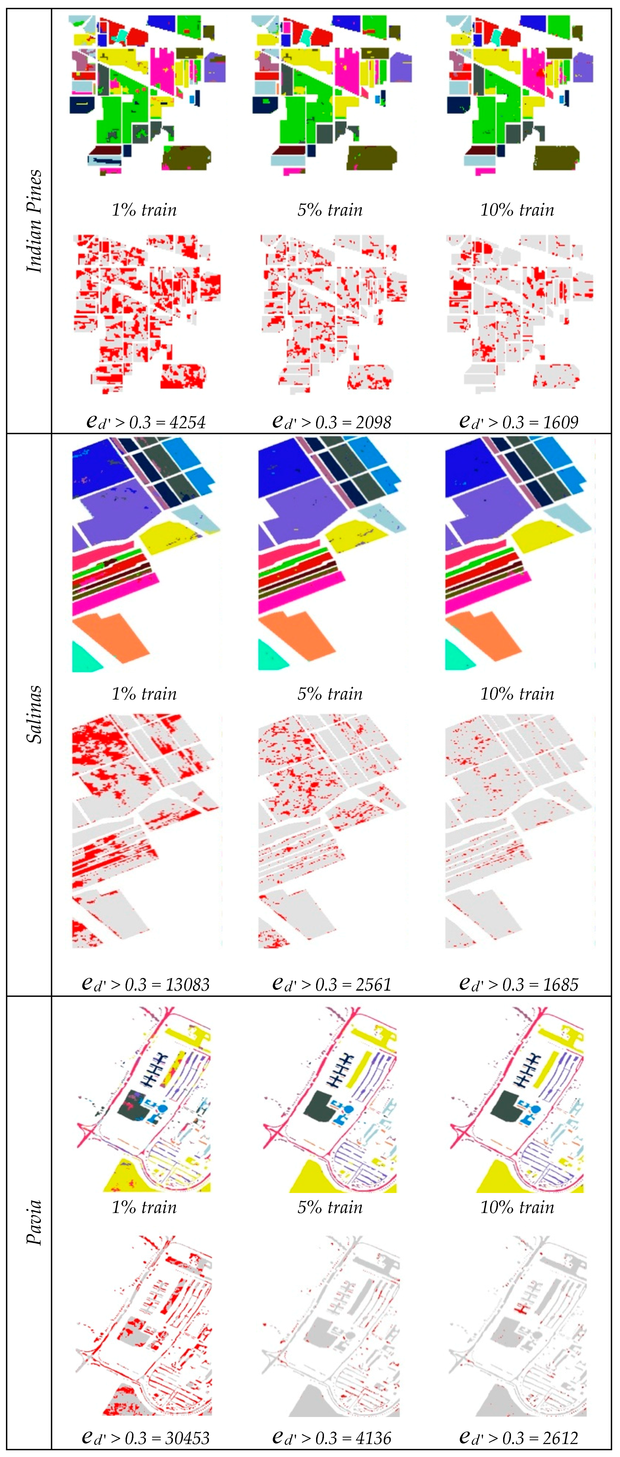
3.2. Uncertainty Mapping

As DoTRules is rule-based, and each unique rule with its specific entropy value corresponds to one or more pixels, it is possible to estimate and map the uncertainty of every unique rule back to those pixels. This is a preliminary product of DoTRules, before assigning a class label to every pixel.
To illustrate the applicability of the entropy map to locate areas belonging to a low versus high classification accuracy, entropy values above and below the applied threshold (ed ’= 0.3, Equation (7)) were mapped to segregate regions which have more reliable and less reliable classification responses (Figure 5). In this way, the DoTRules spatial uncertainty map can facilitate a better understanding of uncertainty in the classified product and the segregation of more and less reliable geographic areas before assigning class labels to every pixel of the test sample dataset. This provides clear spatial insight into the uncertainty of the classification at an early stage of the classification process.
In developing and applying DoTRules, we have found that a larger sample size offers a higher classification accuracy where the number of less reliable rules with higher levels of uncertainty is reduced. Conversely, a smaller sample size, with fewer rules detected in our rule sets, was less able to capture the complexity of the hyperspectral image classification. This is mainly due to the fact that for DoTRules, training samples should be enough to cover all possible forms of rules. Figure 5 demonstrates the rule uncertainty for the Indian Pines, Salinas and Pavia University datasets using 1%, 5% and 10% training sample sizes.

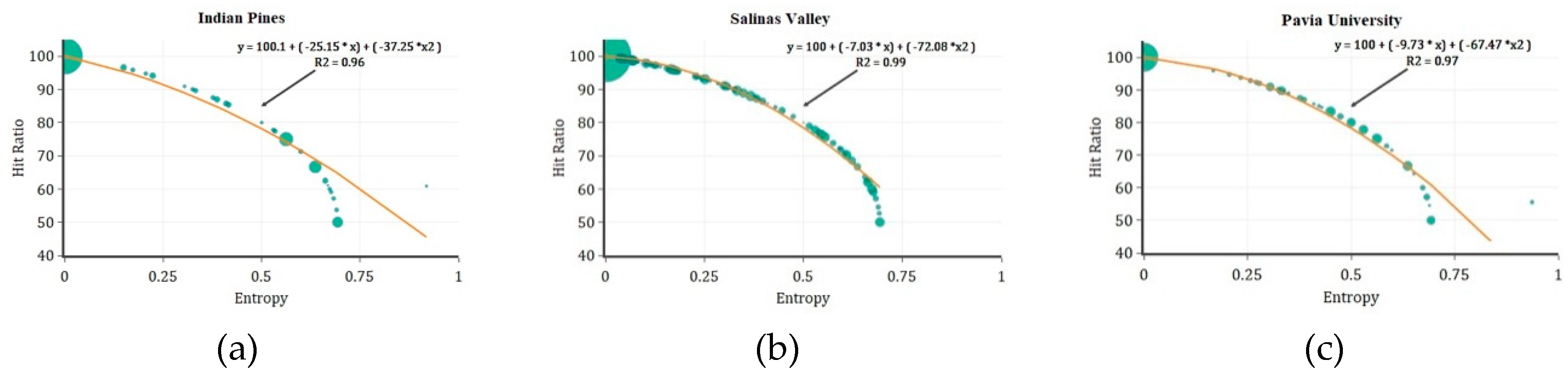
3.3. Correspondence Between Uncertainty and Hit Ratio of Rules

In general, where there is low entropy (i.e., low uncertainty) for a rule within our rule set, the classification also tends to be more accurate. Simply, a lower entropy means there is just one clear answer (the mode class label) for a rule, while a high entropy indicates a more uniform distribution of the map class frequencies for that rule, which indicates a less reliable classification. Plotting hit ratio values against entropy values of every constructed rule among our various rule sets demonstrates that the hit ratio of rules can be defined by a polynomial function of their entropy value (Figure 6), which is supported by a strong coefficient of determination for all three datasets.
To further demonstrate the applicability of DoTRules’ uncertainty product for the anticipation of the rule-exclusive hit ratio, we then applied the derived functions based on the correspondence of the hit ratio and entropy of the training data to predict the hit ratio of rules within the test datasets. The root mean square error (RMSE) values of the predicted hit ratios based on the entropy polynomial function were <1 for all three datasets (Table 2). Table 2 demonstrates that the uncertainty product of DoTRules may be applied to estimate the hit ratio of the classification rules in the context of the hyperspectral image classification.

4. Discussion

In this paper, we have presented a rule-based ensemble framework based on a mean-shift segmentation and uncertainty analysis, referred to as DoTRules (a Dictionary of Trusted Rules), for hyperspectral image classification. DoTRules constructs many rule sets composed of corresponding rules for each pixel in a hyperspectral image to predict the class of the test samples. When applied to different datasets and sample sizes, DoTRules proved to be an effective strategy for the classification of hyperspectral imagery, with promising results compared to other established algorithms. Furthermore, DoTRules enables both rule uncertainty and hit ratio mapping, which is an advantage for the users of classified land-use and land-cover maps created from remote sensing imagery. Below, we discuss improvements in hyperspectral image classification achieved using DoTRules.

4.1. The Overall Accuracy of Classification

According to our results, for all three applied hyperspectral datasets, the DoTRules ensemble framework was more accurate than the other applied classification algorithms for most training sample sizes (Table 1). This is due to the robust rule detection framework using mean-shift segmentation, where Shannon entropy is used to assess the uncertainty of individual rules for classification purpose. Here, the segmentation is done in a way where each DN in each segment (ideally) shares some common trait. This bears similarities with an object-oriented classification that involves the categorization of pixels based on the spatial relationship with the surrounding pixels. While pixel-based classification is exclusively based on the information in each pixel, object-based classification is based on information from a set of similar pixels (i.e., objects or image objects). Image objects are groups of pixels that are similar to one another based on the spectral properties (i.e., colour), size, shape, and texture, as well as context from a neighbourhood surrounding the pixels, in an attempt to mimic the type of analysis done by humans during visual interpretation. In addition, passing segment information to pixels and extracting reliable rules (i.e., low uncertainty rules) using minimum entropy through a voting system further preserves the high classification accuracy, especially when a representative training sample size is applied.
The observed increase in the overall accuracy of DoTRules’ estimates when applying larger sample sizes may be due to an extra number of rules being detected and relatively fewer null records. Rules are very general structures that offer an easily understandable and transparent way to find the most reliable class allocation for a pixel [30]. As opposed to decision trees, every rule corresponds to only one pixel. This is unique to DoTRules and a common criticism of XGboost, RF, RoF, RRF and similar black-box algorithms [76,77]. Users can access all rules and their corresponding information, such as the rule ID, components of a rule (segment class for every selected band), true class label, probability (relative frequency) of every potential class label, rule entropy and hit ratio (accuracy) (Figure 2), while they are always connected to their corresponding pixels. This beneficial trait is highly valued in geoscience and remote sensing applications, especially in the context of land-use and land-cover mapping applications [38,78,79]. To be able to assign every pixel to a map class, each pixel should have at least one matching rule from various rule sets. Logically, the number of recognised rules within each individual rule set will be increased by a consequent increase in the training sample size (i.e., 1% to 10%), while the number of null records derived from unmatched rules between the test and training dataset will be reduced. Therefore, the greater the number of trusted rules, the greater the capability of our proposed framework to allocate test pixels into their true class labels.

4.2. Quantifying and Mapping the Uncertainty of Rules

While a few studies have successfully mapped the uncertainty of classification before image classification [38,80], one strength of DoTRules in hyperspectral image classification is its demonstrated ability to quantify the uncertainty of every identified transition rule using entropy values prior to the final classification (Figure 5). In other words, DoTRules was able to report the uncertainty of rules based on Shannon entropy, independent from the test dataset. The results from different hyperspectral datasets show that the lower the entropy value, the higher the hit ratio (Figure 6). Thus, considering the strong relationship between the entropy and hit ratio, it is possible to apply the entropy values as estimates of the hit ratio. The estimation of the rule uncertainty prior to the classification of a hyperspectral dataset aids in understanding the specific strengths and weaknesses of a classifier dealing with pixels containing a range of spectral information.

4.3. Quantifying Hit Ratio of Rules

DoTRules demonstrated the ability to quantify the rule-exclusive hit ratio using their corresponding entropy values (Table 2). Thus, the uncertainty product based on the entropy values can be applied to segregate areas of less and more reliable prediction independently of the test data availability. Thus, in the absence of a proper test dataset for the validation of classification results, rules’ uncertainty values can be applied to represent their corresponding hit ratio. The collection of reliable ground truths for validation purposes is usually an expensive task in terms of time and economic costs [81]. Consequently, in many cases, it may not be possible to rely on test data to ensure good performance of a classifier. Accordingly, aside from using traditional accuracy metrics as a single number derived from a confusion matrix, mapping and thresholding the rule-exclusive hit ratio in a classification scheme is worthwhile for visualising general patterns of high and low accuracy values within the classified map and quantifying the accuracy of prediction in specific targeted locations.

4.4. Limitations of DoTRules and Future Work

Although the results obtained by DoTRules are encouraging, further comparative experiments with additional hyperspectral imagery datasets should be implemented. This can be more useful with a particular focus on assessing the classification performance at higher levels of disaggregation, such as a class-level accuracy assessment. As some of the required parameters for the DoTRules implementation are subjective, such as 1) the rule uncertainty threshold, 2) the minimum and maximum length of random rules and 3) the optimum number of rule sets, more research may be beneficial in the computational optimisation of DoTRules parameters. Our further work is focusing on the development of more computationally efficient schemes for the ensemble framework.
Another limitation of the proposed ensemble framework is the fact that the proposed framework is less efficient for very low sample sizes (i.e., 1% or less). DoTrules usually needs a larger training set to extract the underlying relationships between variables. This is a common requirement for all ensemble methods except RoF. Although RoF is the best performing algorithm for the 1% sample size of Indian Pines, it benefits from the transformation of the hyperspectral data.

5. Conclusions

We have applied DoTRules—a Dictionary of Trusted Rules—as an innovative ensemble framework for classifying hyperspectral data with high accuracy estimates compared with other popular classification algorithms. DoTRules’ classification accuracy was superior to six other popular and state-of-the-art ensemble and non-ensemble algorithms. In the case of DoTRules, every rule within any rule set can be accessed, and their corresponding uncertainty value may be observed. This feature is unique to DoTRules and the absence of this ability underpins a common criticism of many ensemble algorithms (including many of the algorithms applied here) as black-box classifiers. Furthermore, DoTRules is also capable of quantifying and mapping the uncertainty of these classification rules, prior to the image classification where the uncertainty values can be applied as an estimate of the hit ratio. While the entropy product of DoTRules provides spatial insights, including the location of less reliable classification rules as well as more reliable ones, regardless of the test sample dataset availability, it can also certify and locate less accurate rules using the estimated hit ratio. The spatial exploration of rule uncertainty in hyperspectral image classification is beneficial for the early prediction of success or failure of a classifier in specific geographic locations. The uncertainty maps may also serve to enhance the application of map products by alerting map users to the spatial variation of rules’ hit ratio over the entire mapped region. This, together with the simplicity and accuracy of DoTRules, indicates that the methodology offers new features and is ready for operational use by the remote sensing community.

Author Contributions

Conceptualization, M.S.R.; methodology, M.S.R.; validation, M.S.R. and A.A.; writing—original draft preparation, M.S.R., A.L. and B.A.B.; writing—review and editing, A.L., A.A. and B.A.B.; visualization, M.S.R.; supervision, A.L. and B.A.B.; funding acquisition, B.A.B. All authors read and approved the final manuscript.

Funding

This research was supported by CSIRO Australian Sustainable Agriculture Scholarship (ASAS) as a top-up scholarship to Majid Shadman Roodposhti, a PhD scholar, at the University of Tasmania (RT109121), School of Land and Food.

Acknowledgments

The authors greatly appreciate Maia Angelova Turkedjieva and Ye Zhu, Deakin University, for their suggestions to improve this manuscript. We also thank Monica Cuskelly, Associate Dean (Research), University of Tasmania, for editing the manuscript. We also thank the anonymous reviewers for their valuable comments and suggestions to improve the quality of the paper.

Conflicts of Interest

The authors declare no conflict of interest.

References

  1. Chan, J.C.-W.; Paelinckx, D. Evaluation of random forest and adaboost tree-based ensemble classification and spectral band selection for ecotope mapping using airborne hyperspectral imagery. Remote Sens. Environ. 2008, 112, 2999–3011. [Google Scholar] [CrossRef]
  2. Adep, R.N.; Vijayan, A.P.; Shetty, A.; Ramesh, H. Performance evaluation of hyperspectral classification algorithms on aviris mineral data. Perspect. Sci. 2016, 8, 722–726. [Google Scholar] [CrossRef]
  3. Van der Meer, F.D.; van der Werff, H.M.A.; van Ruitenbeek, F.J.A.; Hecker, C.A.; Bakker, W.H.; Noomen, M.F.; van der Meijde, M.; Carranza, E.J.M.; Smeth, J.B.D.; Woldai, T. Multi- and hyperspectral geologic remote sensing: A review. Int. J. Appl. Earth Obs. Geoinform. 2012, 14, 112–128. [Google Scholar] [CrossRef]
  4. Zarco-Tejada, P.J.; González-Dugo, M.V.; Fereres, E. Seasonal stability of chlorophyll fluorescence quantified from airborne hyperspectral imagery as an indicator of net photosynthesis in the context of precision agriculture. Remote Sens. Environ. 2016, 179, 89–103. [Google Scholar] [CrossRef]
  5. Wakholi, C.; Kandpal, L.M.; Lee, H.; Bae, H.; Park, E.; Kim, M.S.; Mo, C.; Lee, W.-H.; Cho, B.-K. Rapid assessment of corn seed viability using short wave infrared line-scan hyperspectral imaging and chemometrics. Sens. Actuators B Chem. 2018, 255, 498–507. [Google Scholar] [CrossRef]
  6. Rodger, A.; Laukamp, C.; Haest, M.; Cudahy, T. A simple quadratic method of absorption feature wavelength estimation in continuum removed spectra. Remote Sens. Environ. 2012, 118, 273–283. [Google Scholar] [CrossRef]
  7. Chen, F.; Wang, K.; Van de Voorde, T.; Tang, T.F. Mapping urban land cover from high spatial resolution hyperspectral data: An approach based on simultaneously unmixing similar pixels with jointly sparse spectral mixture analysis. Remote Sens. Environ. 2017, 196, 324–342. [Google Scholar] [CrossRef]
  8. Ma, X.; Wang, H.; Wang, J. Semisupervised classification for hyperspectral image based on multi-decision labeling and deep feature learning. ISPRS J. Photogramm. Remote Sens. 2016, 120, 99–107. [Google Scholar] [CrossRef]
  9. Huang, K.; Li, S.; Kang, X.; Fang, L. Spectral–spatial hyperspectral image classification based on knn. Sens. Imaging 2015, 17, 1. [Google Scholar] [CrossRef]
  10. Khodadadzadeh, M.; Li, J.; Plaza, A.; Bioucas-Dias, J.M. A subspace-based multinomial logistic regression for hyperspectral image classification. IEEE Geosci. Remote Sens. Lett. 2014, 11, 2105–2109. [Google Scholar] [CrossRef]
  11. Peng, J.; Zhang, L.; Li, L. Regularized set-to-set distance metric learning for hyperspectral image classification. Pattern Recognit. Lett. 2016, 83, 143–151. [Google Scholar] [CrossRef]
  12. Goel, P.K.; Prasher, S.O.; Patel, R.M.; Landry, J.A.; Bonnell, R.B.; Viau, A.A. Classification of hyperspectral data by decision trees and artificial neural networks to identify weed stress and nitrogen status of corn. Comput. Electron. Agric. 2003, 39, 67–93. [Google Scholar] [CrossRef]
  13. Shao, Y.; Sang, N.; Gao, C.; Ma, L. Probabilistic class structure regularized sparse representation graph for semi-supervised hyperspectral image classification. Pattern Recognit. 2017, 63, 102–114. [Google Scholar] [CrossRef]
  14. Zhong, Y.; Zhang, L. An adaptive artificial immune network for supervised classification of multi-/hyperspectral remote sensing imagery. IEEE Trans. Geosci. Remote Sens. 2012, 50, 894–909. [Google Scholar] [CrossRef]
  15. Reshma, R.; Sowmya, V.; Soman, K.P. Dimensionality reduction using band selection technique for kernel based hyperspectral image classification. Procedia Comput. Sci. 2016, 93, 396–402. [Google Scholar] [CrossRef]
  16. Naidoo, L.; Cho, M.A.; Mathieu, R.; Asner, G. Classification of savanna tree species, in the greater kruger national park region, by integrating hyperspectral and lidar data in a random forest data mining environment. ISPRS J. Photogramm. Remote Sens. 2012, 69, 167–179. [Google Scholar] [CrossRef]
  17. Kayabol, K.; Kutluk, S. Bayesian classification of hyperspectral images using spatially-varying gaussian mixture model. Digit. Signal Process. 2016, 59, 106–114. [Google Scholar] [CrossRef]
  18. Gao, L.; Li, J.; Khodadadzadeh, M.; Plaza, A.; Zhang, B.; He, Z.; Yan, H. Subspace-based support vector machines for hyperspectral image classification. IEEE Geosci. Remote Sens. Lett. 2015, 12, 349–353. [Google Scholar]
  19. Feng, J.; Jiao, L.; Liu, F.; Sun, T.; Zhang, X. Unsupervised feature selection based on maximum information and minimum redundancy for hyperspectral images. Pattern Recognit. 2016, 51, 295–309. [Google Scholar] [CrossRef]
  20. Guo, B.; Gunn, S.R.; Damper, R.I.; Nelson, J.D. Band selection for hyperspectral image classification using mutual information. IEEE Geosci. Remote Sens. Lett. 2006, 3, 522–526. [Google Scholar] [CrossRef]
  21. Awad, M. Sea water chlorophyll-a estimation using hyperspectral images and supervised artificial neural network. Ecol. Inform. 2014, 24, 60–68. [Google Scholar] [CrossRef]
  22. Yu, S.; Jia, S.; Xu, C. Convolutional neural networks for hyperspectral image classification. Neurocomputing 2017, 219, 88–98. [Google Scholar] [CrossRef]
  23. Li, Y.; Xie, W.; Li, H. Hyperspectral image reconstruction by deep convolutional neural network for classification. Pattern Recognit. 2017, 63, 371–383. [Google Scholar] [CrossRef]
  24. Castelvecchi, D. Can we open the black box of ai? Nat. News 2016, 538, 20. [Google Scholar] [CrossRef] [PubMed]
  25. Goodfellow, I.J.; Erhan, D.; Carrier, P.L.; Courville, A.; Mirza, M.; Hamner, B.; Cukierski, W.; Tang, Y.; Thaler, D.; Lee, D.-H.; et al. Challenges in representation learning: A report on three machine learning contests. Neural Netw. 2015, 64, 59–63. [Google Scholar] [CrossRef] [PubMed] [Green Version]
  26. Ayerdi, B.; Marqués, I.; Graña, M. Spatially regularized semisupervised ensembles of extreme learning machines for hyperspectral image segmentation. Neurocomputing 2015, 149, 373–386. [Google Scholar] [CrossRef]
  27. Uslu, F.S.; Binol, H.; Ilarslan, M.; Bal, A. Improving svdd classification performance on hyperspectral images via correlation based ensemble technique. Opt. Lasers Eng. 2017, 89, 169–177. [Google Scholar] [CrossRef]
  28. Ayerdi, B.; Graña, M. Hyperspectral image nonlinear unmixing and reconstruction by elm regression ensemble. Neurocomputing 2016, 174, 299–309. [Google Scholar] [CrossRef]
  29. Tseng, M.-H.; Chen, S.-J.; Hwang, G.-H.; Shen, M.-Y. A genetic algorithm rule-based approach for land-cover classification. ISPRS J. Photogramm. Remote Sens. 2008, 63, 202–212. [Google Scholar] [CrossRef]
  30. Russell, S.J.; Norvig, P.; Canny, J.F.; Malik, J.M.; Edwards, D.D. Artificial Intelligence: A Modern Approach; Prentice Hall: Upper Saddle River, NJ, USA, 2003; Volume 2. [Google Scholar]
  31. Bauer, T.; Steinnocher, K. Per-parcel land use classification in urban areas applying a rule-based technique. GeoBIT/GIS 2001, 6, 24–27. [Google Scholar]
  32. Benediktsson, J.A.; Garcia, X.C.; Waske, B.; Chanussot, J.; Sveinsson, J.R.; Fauvel, M. Ensemble methods for classification of hyperspectral data. In Proceedings of the IEEE International Geoscience and Remote Sensing Symposium (IGARSS 2008), Boston, MA, USA, 6–11 July 2008; IEEE: Piscataway, NJ, USA, 2008; pp. 62–65. [Google Scholar]
  33. Ceamanos, X.; Waske, B.; Benediktsson, J.A.; Chanussot, J.; Fauvel, M.; Sveinsson, J.R. A classifier ensemble based on fusion of support vector machines for classifying hyperspectral data. Int. J. Image Data Fusion 2010, 1, 293–307. [Google Scholar] [CrossRef] [Green Version]
  34. Xia, J.; Ghamisi, P.; Yokoya, N.; Iwasaki, A. Random forest ensembles and extended multiextinction profiles for hyperspectral image classification. IEEE Trans. Geosci. Remote Sens. 2018, 56, 202–216. [Google Scholar] [CrossRef]
  35. Rokach, L. Ensemble-based classifiers. Artif. Intell. Rev. 2010, 33, 1–39. [Google Scholar] [CrossRef]
  36. Shadman, M.; Aryal, J.; Bryan, B. Dotrules: A novel method for calibrating land-use/cover change models using a dictionary of trusted rules. In Proceedings of the MODSIM2017, 22nd International Congress on Modelling and Simulation, Hobart, Australia, 3–8 December 2017; Syme, G., Hatton MacDonald, D., Fulton, B., Piantadosi, J., Eds.; Hobart, TAS, Australia, 2017; p. 508. [Google Scholar]
  37. Roodposhti, M.S.; Aryal, J.; Bryan, B.A. A novel algorithm for calculating transition potential in cellular automata models of land-use/cover change. Environ. Model. Softw. 2019, 112, 70–81. [Google Scholar] [CrossRef]
  38. Khatami, R.; Mountrakis, G.; Stehman, S.V. Mapping per-pixel predicted accuracy of classified remote sensing images. Remote Sens. Environ. 2017, 191, 156–167. [Google Scholar] [CrossRef] [Green Version]
  39. Congalton, R.G. A review of assessing the accuracy of classifications of remotely sensed data. Remote Sens. Environ. 1991, 37, 35–46. [Google Scholar] [CrossRef]
  40. Georganos, S.; Grippa, T.; Vanhuysse, S.; Lennert, M.; Shimoni, M.; Wolff, E. Very high resolution object-based land use-land cover urban classification using extreme gradient boosting. IEEE Geosci. Remote Sens. Lett. 2018, 15, 607–611. [Google Scholar] [CrossRef]
  41. Loggenberg, K.; Strever, A.; Greyling, B.; Poona, N. Modelling water stress in a shiraz vineyard using hyperspectral imaging and machine learning. Remote Sens. 2018, 10, 202. [Google Scholar] [CrossRef]
  42. Crawford, M.M.; Ham, J.; Chen, Y.; Ghosh, J. Random forests of binary hierarchical classifiers for analysis of hyperspectral data. In Proceedings of the 2003 IEEE Workshop on Advances in Techniques for Analysis of Remotely Sensed Data, Greenbelt, MD, USA, 27–28 October 2003; IEEE: Piscataway, NJ, USA, 2003; pp. 337–345. [Google Scholar]
  43. Gislason, P.O.; Benediktsson, J.A.; Sveinsson, J.R. Random forests for land cover classification. Pattern Recognit. Lett. 2006, 27, 294–300. [Google Scholar] [CrossRef]
  44. Ham, J.; Chen, Y.; Crawford, M.M.; Ghosh, J. Investigation of the random forest framework for classification of hyperspectral data. IEEE Trans. Geosci. Remote Sens. 2005, 43, 492–501. [Google Scholar] [CrossRef] [Green Version]
  45. Lawrence, R.L.; Wood, S.D.; Sheley, R.L. Mapping invasive plants using hyperspectral imagery and breiman cutler classifications (randomforest). Remote Sens. Environ. 2006, 100, 356–362. [Google Scholar] [CrossRef]
  46. Xia, J.; Du, P.; He, X.; Chanussot, J. Hyperspectral remote sensing image classification based on rotation forest. IEEE Geosci. Remote Sens. Lett. 2014, 11, 239–243. [Google Scholar] [CrossRef]
  47. Xia, J.; Chanussot, J.; Du, P.; He, X. Spectral—Spatial classification for hyperspectral data using rotation forests with local feature extraction and markov random fields. IEEE Trans. Geosci. Remote Sens. 2015, 53, 2532–2546. [Google Scholar] [CrossRef]
  48. Xia, J.; Falco, N.; Benediktsson, J.A.; Chanussot, J.; Du, P. Class-separation-based rotation forest for hyperspectral image classification. IEEE Geosci. Remote Sens. Lett. 2016, 13, 584–588. [Google Scholar] [CrossRef]
  49. Feng, W.; Bao, W. Weight-based rotation forest for hyperspectral image classification. IEEE Geosci. Remote Sens. Lett. 2017, 14, 2167–2171. [Google Scholar] [CrossRef]
  50. Izquierdo-Verdiguier, E.; Zurita-Milla, R.; Rolf, A. On the use of guided regularized random forests to identify crops in smallholder farm fields. In Proceedings of the 2017 9th International Workshop on the Analysis of Multitemporal Remote Sensing Images (MultiTemp), Brugge, Belgium, 27–29 June 2017; IEEE: Piscataway, NJ, USA, 2017; pp. 1–3. [Google Scholar]
  51. Mureriwa, N.; Adam, E.; Sahu, A.; Tesfamichael, S. Examining the spectral separability of prosopis glandulosa from co-existent species using field spectral measurement and guided regularized random forest. Remote Sens. 2016, 8, 144. [Google Scholar] [CrossRef]
  52. Fauvel, M.; Benediktsson, J.A.; Chanussot, J.; Sveinsson, J.R. Spectral and spatial classification of hyperspectral data using svms and morphological profiles. IEEE Trans. Geosci. Remote Sens. 2008, 46, 3804–3814. [Google Scholar] [CrossRef]
  53. Tarabalka, Y.; Fauvel, M.; Chanussot, J.; Benediktsson, J.A. Svm-and mrf-based method for accurate classification of hyperspectral images. IEEE Geosci. Remote Sens. Lett. 2010, 7, 736–740. [Google Scholar] [CrossRef]
  54. Bazi, Y.; Melgani, F. Toward an optimal svm classification system for hyperspectral remote sensing images. IEEE Trans. Geosci. Remote Sens. 2006, 44, 3374–3385. [Google Scholar] [CrossRef]
  55. Cui, M.; Prasad, S. Class-dependent sparse representation classifier for robust hyperspectral image classification. IEEE Trans. Geosci. Remote Sens. 2015, 53, 2683–2695. [Google Scholar] [CrossRef]
  56. Lv, Q.; Niu, X.; Dou, Y.; Wang, Y.; Xu, J.; Zhou, J. Hyperspectral image classification via kernel extreme learning machine using local receptive fields. In Proceedings of the 2016 IEEE International Conference on Image Processing (ICIP), Phoenix, AZ, USA, 25–28 September 2016; IEEE: Piscataway, NJ, USA, 2016; pp. 256–260. [Google Scholar]
  57. Li, J.; Xi, B.; Li, Y.; Du, Q.; Wang, K. Hyperspectral classification based on texture feature enhancement and deep belief networks. Remote Sens. 2018, 10, 396. [Google Scholar] [CrossRef]
  58. Chen, Y.; Zhao, X.; Jia, X. Spectral–spatial classification of hyperspectral data based on deep belief network. IEEE J. Sel. Top. Appl. Earth Obs. Remote Sens. 2015, 8, 2381–2392. [Google Scholar] [CrossRef]
  59. Breiman, L. Bagging predictors. Mach. Learn. 1996, 24, 123–140. [Google Scholar] [CrossRef] [Green Version]
  60. Breiman, L. Random forests. Mach. Learn. 2001, 45, 5–32. [Google Scholar] [CrossRef]
  61. Roodposhti, M.S.; Aryal, J.; Pradhan, B. A novel rule-based approach in mapping landslide susceptibility. Sensors 2019, 19, 2274. [Google Scholar] [CrossRef]
  62. R Core Team. R: A Language and Environment for Statistical Computing; R Foundation for Statistical Computing: Vienna, Austria, 2017. [Google Scholar]
  63. Cheng, Y. Mean shift, mode seeking, and clustering. IEEE Trans. Pattern Anal. Mach. Intell. 1995, 17, 790–799. [Google Scholar] [CrossRef]
  64. Fukunaga, K.; Hostetler, L. The estimation of the gradient of a density function, with applications in pattern recognition. IEEE Trans. Inf. Theory 1975, 21, 32–40. [Google Scholar] [CrossRef]
  65. Silverman, B.W. Density Estimation for Statistics and Data Analysis; Routledge: Abingdon, UK, 2018. [Google Scholar]
  66. Carreira-Perpinán, M.A. A review of mean-shift algorithms for clustering. arXiv 2015, arXiv:1503.00687. [Google Scholar]
  67. Huband, J.M.; Bezdek, J.C.; Hathaway, R.J. Bigvat: Visual assessment of cluster tendency for large data sets. Pattern Recognit. 2005, 38, 1875–1886. [Google Scholar] [CrossRef]
  68. Shannon, C.E. A mathematical theory of communication. ACM SIGMOBILE Mob. Comput. Commun. Rev. 2001, 5, 3–55. [Google Scholar] [CrossRef]
  69. Chen, T.; Guestrin, C. Xgboost: A scalable tree boosting system. In Proceedings of the 22nd ACM Sigkdd International Conference on Knowledge Discovery and Data Mining, San Francisco, CA, USA, 13–17 August 2016; ACM: New York, NY, USA, 2016; pp. 785–794. [Google Scholar]
  70. Mahapatra, D. Analyzing training information from random forests for improved image segmentation. IEEE Trans. Image Process. 2014, 23, 1504–1512. [Google Scholar] [CrossRef] [PubMed]
  71. Golipour, M.; Ghassemian, H.; Mirzapour, F. Integrating hierarchical segmentation maps with mrf prior for classification of hyperspectral images in a bayesian framework. IEEE Trans. Geosci. Remote Sens. 2016, 54, 805–816. [Google Scholar] [CrossRef]
  72. Kuhn, M. Caret package. J. Stat. Softw. 2008, 28, 1–26. [Google Scholar]
  73. Yang, C.; Tan, Y.; Bruzzone, L.; Lu, L.; Guan, R. Discriminative feature metric learning in the affinity propagation model for band selection in hyperspectral images. Remote Sens. 2017, 9, 782. [Google Scholar] [CrossRef]
  74. Kianisarkaleh, A.; Ghassemian, H. Nonparametric feature extraction for classification of hyperspectral images with limited training samples. ISPRS J. Photogramm. Remote Sens. 2016, 119, 64–78. [Google Scholar] [CrossRef]
  75. Luo, F.; Huang, H.; Duan, Y.; Liu, J.; Liao, Y. Local geometric structure feature for dimensionality reduction of hyperspectral imagery. Remote Sens. 2017, 9, 790. [Google Scholar] [CrossRef]
  76. Palczewska, A.; Palczewski, J.; Robinson, R.M.; Neagu, D. Interpreting random forest models using a feature contribution method. In Proceedings of the 2013 IEEE 14th International Conference on Information Reuse and Integration (IRI), San Francisco, CA, USA, 14–16 August 2013; IEEE: Piscataway, NJ, USA, 2013; pp. 112–119. [Google Scholar] [Green Version]
  77. Gislason, P.O.; Benediktsson, J.A.; Sveinsson, J.R. Random forest classification of multisource remote sensing and geographic data. In Proceedings of the 2004 IEEE International Geoscience and Remote Sensing Symposium, Anchorage, AK, USA, 20–24 September 2004; IEEE: Piscataway, NJ, USA, 2004; pp. 1049–1052. [Google Scholar]
  78. Yang, X.; Chen, L.; Li, Y.; Xi, W.; Chen, L. Rule-based land use/land cover classification in coastal areas using seasonal remote sensing imagery: A case study from Lianyungang city, China. Environ. Monit. Assess. 2015, 187, 449. [Google Scholar] [CrossRef] [PubMed]
  79. Lucas, R.; Rowlands, A.; Brown, A.; Keyworth, S.; Bunting, P. Rule-based classification of multi-temporal satellite imagery for habitat and agricultural land cover mapping. ISPRS J. Photogramm. Remote Sens. 2007, 62, 165–185. [Google Scholar] [CrossRef]
  80. Bryan, B.A.; Barry, S.; Marvanek, S. Agricultural commodity mapping for land use change assessment and environmental management: An application in the Murray–darling basin, Australia. J. Land Use Sci. 2009, 4, 131–155. [Google Scholar] [CrossRef]
  81. Bruzzone, L.; Prieto, D.F. Unsupervised retraining of a maximum likelihood classifier for the analysis of multitemporal remote sensing images. IEEE Trans. Geosci. Remote Sens. 2001, 39, 456–460. [Google Scholar] [CrossRef] [Green Version]
Figure 1. A visual illustration of different categories of machine learning methods used for image classification.
Remotesensing 11 02057 g001
Figure 2. Schematic demonstration of (a,b) reliable and (c,d) unreliable rules extracted using DoTRules. The black circles represent the segment values of randomly selected spectral bands composing different rules for one target pixel. Considering rule sets number #1 and #2, the latter will have more impact in combining votes due to its larger length.
Remotesensing 11 02057 g002
Figure 3. False color composites and ground truth images of the datasets used to illustrate the image classification using DoTRules, including the (a,b) Indian Pines, (c,d) Salinas and (e,f) Pavia University datasets.
Remotesensing 11 02057 g003
Figure 4. The mean spectral signatures of the (a) Indian Pines, (b) Salinas Valley and (c) Pavia University datasets.
Remotesensing 11 02057 g004
Figure 5. The DoTRules classification results and estimated pixel-based e d , for the Indian Pines, Salinas and Pavia datasets. The red pixels show the location of unreliable rules according to entropy thresholding ( e d > 0.3, for α = 0.05), while the grey pixels are reliable rules above the threshold. The red pixels are counted for each sample size.
Remotesensing 11 02057 g005
Figure 6. Entropy versus the hit ratio of rules for the (a) Indian Pines, (b) Salinas Valley and (c) Pavia University dataset 10% training sample sizes. The bubble sizes show the frequency of each rule among all corresponding rules from different rule sets before combining votes.
Remotesensing 11 02057 g006
Table 1. The accuracy assessment results of three applied datasets, including the overall accuracy (OA%) and kappa coefficient (κ) for all applied methods including support vector machine (SVM), deep belief network (DBN), extreme gradient boosting (XGBoost), random forest (RF), rotation forests (RoFs), regularised random forest (RRF), as well as Dictionary of Trusted Rules (DoTRules). The maximum values are highlighted in bold.
TrainTestSVMDBNXGboostRFRoFRRFDoTRules
Indian Pines1%50%62.256.052.964.870.558.868.6
0.5580.4860.4530.5930.6500.5210.640
5%50%75.073.069.869.377.964.687.3
0.7080.6890.6560.6440.7250.5880.855
10%50%81.078.675.073.484.972.393.2
0.7810.7550.7100.6930.7880.6750.928
Salinas1%50%90.687.789.086.689.988.191.5
0.8950.8620.8770.8500.8810.8670.906
5%50%92.392.290.890.391.990.197.2
0.9140.9130.8980.8920.9080.8880.969
10%50%93.392.392.191.592.990.698.7
0.9250.9140.9120.9050.9180.8950.986
Pavia1%50%92.086.781.681.884.981.679.1
0.8930.8200.7480.7490.7900.7320.720
5%50%93.093.088.787.688.287.393.1
0.9070.9060.8490.8330.8710.8170.909
10%50%94.494.291.289.491.488.996.2
0.9250.9200.8820.8570.8950.8500.951
Table 2. The prediction of rules’ hit ratio based on the corresponding entropy values for a 10% training sample size.
DatasetRR-Squaredp-ValueTrain RMSE Test RMSE
Indian Pines0.9780.9582.20 × 10−160.32610.0972
Salinas Valley0.9960.9932.20 × 10−160.01950.1087
Pavia University0.9850.9712.20 × 10−160.01420.0628

