Article

Detection of Small Target Using Schatten 1/2 Quasi-Norm Regularization with Reweighted Sparse Enhancement in Complex Infrared Scenes

College of Electronic and Information Engineering, Nanjing University of Aeronautics and Astronautics, Nanjing 211106, China
*
Author to whom correspondence should be addressed.
Remote Sens. 2019, 11(17), 2058; https://0-doi-org.brum.beds.ac.uk/10.3390/rs11172058
Submission received: 19 June 2019 / Revised: 19 August 2019 / Accepted: 28 August 2019 / Published: 2 September 2019
(This article belongs to the Section Remote Sensing Image Processing)

Abstract

:
In uniform infrared scenes with single sparse high-contrast small targets, most existing small target detection algorithms perform well. However, when encountering multiple and/or structurally sparse targets in complex backgrounds, these methods potentially lead to high missing and false alarm rate. In this paper, a novel and robust infrared single-frame small target detection is proposed via an effective integration of Schatten 1/2 quasi-norm regularization and reweighted sparse enhancement (RS1/2NIPI). Initially, to achieve a tighter approximation to the original low-rank regularized assumption, a nonconvex low-rank regularizer termed as Schatten 1/2 quasi-norm (S1/2N) is utilized to replace the traditional convex-relaxed nuclear norm. Then, a reweighted l1 norm with adaptive penalty serving as sparse enhancement strategy is employed in our model for suppressing non-target residuals. Finally, the small target detection task is reformulated as a problem of nonconvex low-rank matrix recovery with sparse reweighting. The resulted model falls into the workable scope of inexact augment Lagrangian algorithm, in which the S1/2N minimization subproblem can be efficiently solved by the designed softening half-thresholding operator. Extensive experimental results on several real infrared scene datasets validate the superiority of the proposed method over the state-of-the-arts with respect to background interference suppression and target extraction.

Graphical Abstract

1. Introduction

Along with the advance of infrared imaging technology, small target detection has been attracting great research interests in infrared search and tracking applications, such as precision guidance, defense early warning, and maritime target searching [1,2]. The efficient and robust performance of detection has an important role to play in these applications. However, small targets may be buried in complex infrared scenes with low signal-to-clutter ratios deriving from high bright noise and strong thermal radiation clutters [3]. And they tend to be weak and/or even negligibly small without concrete shape and discriminating textures owing to a long distance between projected targets and imaging sensor [4]. Additionally, there are not enough features in infrared scenes to be incorporated into the designed detection method. Therefore, these limitations make small target detection with high performance full of difficulties and challenges.
Many approaches have been reported for addressing these issues, which roughly include two classes of mainstream detection methods: sequential detection [5,6] and single-frame detection [7,8]. Traditional sequential detection methods are driven by prior information such as target trajectory, velocity and shape, and essentially utilize the adjacent inter-frame knowledge. However, the prior knowledge in inter-frame is hard to guarantee in practical infrared search and tracking systems. Although sequential methods perform well for infrared scenes with motionless background and continuous target in adjacent frame, they may not be ideal for some real-time applications. Because all of frame of sequences must be stored in memory during detection process which not only requires more memory but also incurs high time consuming. So single-frame detection methods are of importance and have been employed more widely due to fewer requirements of prior information and easy implement. The previously proposed single-frame detection methods could be roughly categorized as four classes: filtering method, saliency-based method, classification-based method and nonlocal self-correlation-based method.
The small target detection can be completed by filtering manner according to the fact that uniform infrared background occupying low frequency part presents spatial consistency and small target dominating high frequency region are usually considered as breaking point. The classical filtering methods include Max-mean and Max-median filters [9], two-dimensional least mean square (TDLMS) filter [10,11,12], TopHat [13,14], multiscale directional filter [15] and so on. However, the detection results in these methods are often undesirable due to the sensitivity to the strong edges of heavy cloud or ocean wave clutters.
The saliency-based methods aim to depict the local mutation or complex degree under the assumption on the significant regional changes caused by small targets. Chen et al. [16] provided a clue to simply use local contrast measurement as enhancement factor to pop out small targets and suppress background. After that, there are a series of improved schemes proposed one after another, such as improved/novel local contrast method (ILCM/NLCM) [17,18], relative local contrast measure (RLCM) [19], local saliency map (LSM) [20], weighted local difference measure (WLDM) [21], multiscale patch-based contrast measure (MPCM) [22] and its improved versions [23,24]. Furthermore, the local entropy quantifying the complex degree of local gray distribution has been absorbed into the local contrast method to highlight small targets [25,26]. These methods have achieved high detection probability against the background with higher target contrast. However, some strong interferences which present a similar or even higher contrast to small target would be remined as targets in the saliency-based methods, resulting in high false alarm.
Some methods convert the detection problem into a binary classification problem. They commonly use multiple characteristic of background clutters to train the background classifier or exploit target sample label to search real target among suspicious targets, for example neural networks [27,28], support vector machine [29] and random walker [30,31]. However, due to excessive dependence on training samples or label selection, these methods are hardly adapted readily to some practical cases containing heavy clutters and strong edges. The major reason lies in that infrared backgrounds in real scenes are not only complex but variable. The finite training samples could impossibly cover all background characteristics. On the other hand, inaccurate sample labels may lead to false detection.
The methods exploiting nonlocal self-correlation property assume that all background patches can be represent by a single subspace or a mixture of low-rank subspace clusters. Along this clue, Gao et al. [32] first proposed infrared patch-image (IPI) model via local patch construction, and then transformed target-background detection to recover sparse and low-rank matrices. IPI model have robust and prominent detection performance when facing general scenes. But some weaknesses still obstruct its application in real world, such as the biased background estimation under nuclear norm regularization, the computationally expensive iterative process and the global constant sparse penalty parameter. To solve these problems, Guo et al. [33] suggested to employ a reweighted robust principal analysis model (ReWIPI). Dai et al. [34] and Zhang et al. [35] came up with a reweighted infrared patch-tensor (RIPT) model in which the local and nonlocal prior were integrated to adjust the constant sparse penalty parameter. Moreover, some methods used the multi-space property as structure measure to give a more exact background description, such as stable multi-space learning (SMSL) [36], low-rank and sparse representation model [37].

Motivation

The detection performance of the low-rank recovery-based methods have a great boost against different scenes. However, these methods work inefficiently when facing complex background with multiple and/or structurally sparse targets, resulting in high missing or false alarm. According to our observations, the intrinsic reason lies in the convex relaxation of rank function and l0-norm. First, the nuclear norm is the summation of all singular values rather than treating them as equally as rank function, which will cause biased estimator because of its over-shrinkage effect [38]. The inexact estimation may lead to a phenomenon that a few strong edges or salient outliers are very likely to be treated as target-like components and separated into the target image, causing false alarm. Besides, due to the overlapping-patch mechanism of IPI model, when there are multiple structurally sparse targets in infrared scenes, these targets may show low-rank characteristic to some extent. Then the targets will be considered as background components and restored to the infrared background, causing missing alarm. Second, the l1 norm is employed to constraint the target patch-image, clearly denoting that small targets are sparse enough as pixel-wise structure. However, when encountering structurally sparse targets that are ubiquitous in real scenes, it is unavoidable to over-shrink the targets under over-emphasizing on the sparsity. That would damage the integrity of targets to a certain extent or even result in missing alarm. Lastly, some methods might be computationally expensive due to the slow convergence rate. To tackle the above problems, many efforts have been concentrated on using nonconvex regularization instead of convex surrogates of the original nuclear function. Some popular nonconvex regularizers include log-sum penalty [38], truncated nuclear norm [39], partial sum minimization of singular values [40] and Schatten p quasi-norm [41], and so on. Especially, Dai et al. [42] used the partial sum minimization of singular values replacing the nuclear nom minimization to improve the small target detection rate. However, for this method, it is difficult to estimate a suitable rank to achieve exact detection in real situations. Zhang et al. [43] proposed a non-convex rank approximation minimization method (NRAM) combining γ -norm low-rank approximation with l2,1-norm for detecting small target. This method is workable in complex scene with single point-wise target. Nevertheless, it is unsuitable for the sparse structurally target due to the excessive approximation of the γ -norm minimization. Zhang et al. [44] used the lp-norm to constrain the target patch-image for better separating targets, but the index p should be selected manually.
Motivated by the above observations, this paper presents a new scheme combining the Schatten 1/2 quasi-norm (S1/2N) and reweighted sparse enhancement to efficiently discriminate small targets from diversely complex infrared scenes. The main ideas and contributions of the proposed method contain threefold.
(1)
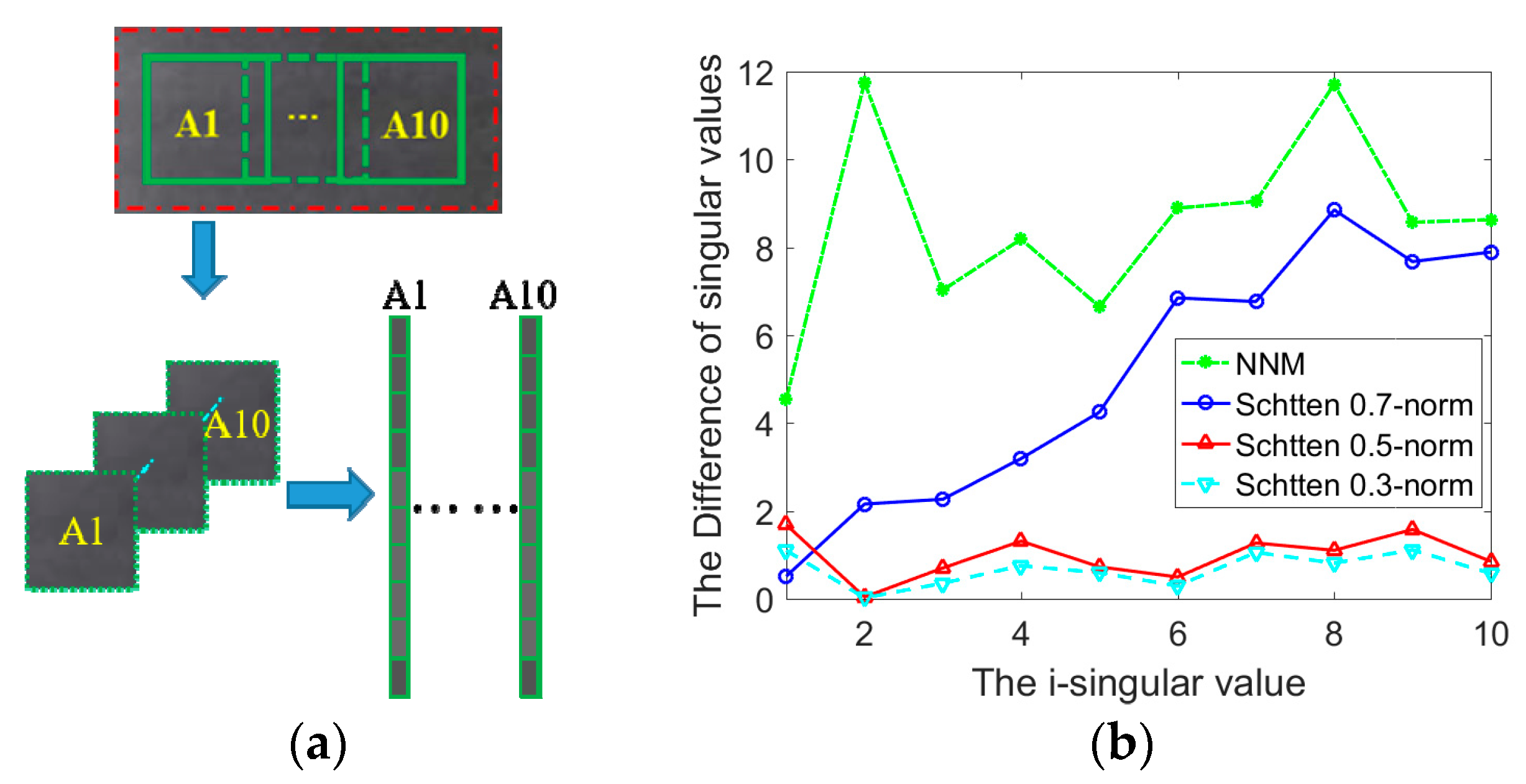
Inspired by the nonconvex low-rank approximation, we use S1/2N regularizer, instead of the traditional nuclear norm, to constrain the background patch-image. The nonconvex regularizer could achieve a tighter approximation of original rank function, obtaining more accurate background estimation.
(2)
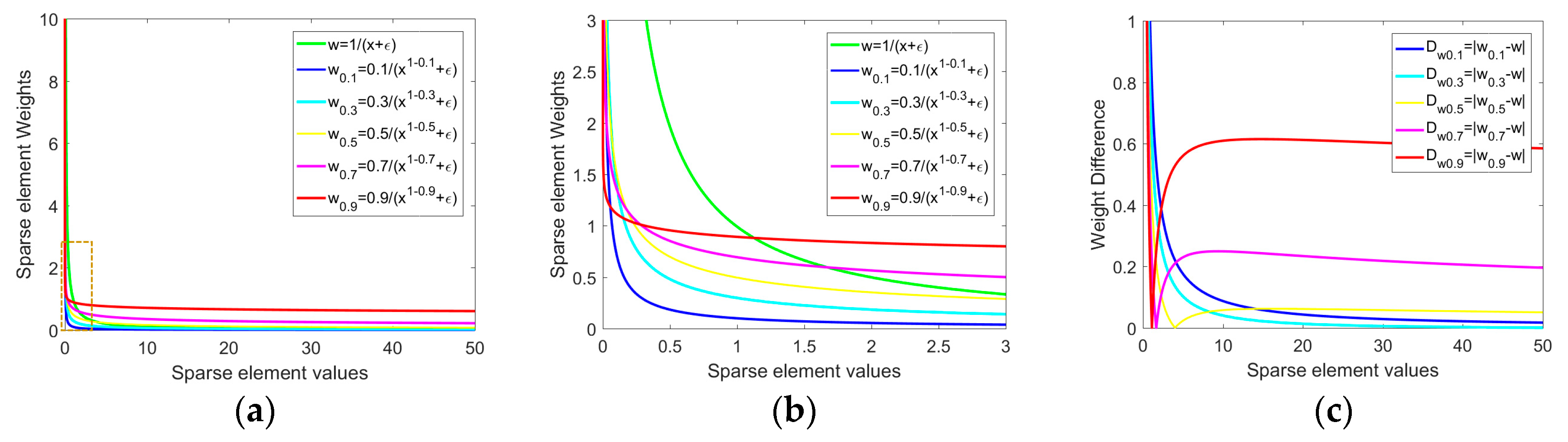
In order to further improve the accuracy of target detection, an entry-wise weight that is different from the traditional weight is formulated. The entry-wise weight benefits to suppress the remaining salient outliers and preserve the target structure.
(3)
The resulted model, called reweighted S1/2N regularization infrared patch-image (RS1/2NIPI), is solved by an effective iterative algorithm based on Alternating Direction Method of Multipliers (ADMM). For the subproblem of S1/2N minimization (S1/2NM), we design a softening half-thresholding algorithm to solve it.
Extensive experimental tests on several real datasets illustrate that the proposed method outperforms other state-of-the-art methods in terms of both the quantitative evaluation and the qualitative comparison. The remaining content of this paper is organized as follows. In Section 2, the IPI model is described in detail. In Section 3, we present a low-rank model based on the Schatten 1/2-norm constraint and further propose the reweighted S1/2NIPI model. In Section 4, the detailed solution of the proposed reweighted model is provided. In Section 5, we display the performance evaluation of the proposed model in detail. The conclusion of this paper is given in Section 6.

2. IPI Model

Infrared images are always contaminated in the acquisition process by a mixture of different kinds of noise and thermal radiation, degrading the image quality seriously. Generally, the impaired infrared image can be modeled as:
f D = f A ( x , y ) + f E ( x , y ) + f N ( x , y )
where f D , f A , f E , f N and ( x , y ) are the original infrared image, the target image, the background image, the random noise image and the pixel location, respectively.
According to Ref. [32], the Infrared Patch-Image model is formulated as:
D = A + E + N
where D, A, E, N are the original infrared patch-image, the background patch-image, the target patch-image, and the noise patch-image, respectively.
Assuming that the nonlocal background patches have significant correlation in an infrared image, the constructed patch-image often presents low-rank property. Hence, the background patch-image vectorized by the overlapping patches can be well regularized by low-rank constraint. For better observation, Figure 1 shows the global and local low-rank property of a representative infrared background patch-image. From the figures, it is clearly that whether the whole patch-image or the local patch-image, the singular values of their constructed matrices rapidly decrease to zero. Undoubtedly, this fully conforms to the hypothesis of low-rank property of the background patch-image. Additionally, the small target usually takes up less than 9 × 9 on a whole image. Thus, it is rational to assume that the target patch-image has sparseness. Under the assumption on the self-correlation of background patch-image and the sparsity of the target patch-image, IPI based detection model converts the small target detection task into an optimization problem recovering low-rank and sparse matrices. Then the detection problem is reformulated as the following convex optimization:
min A , E | | A | | + λ | | E | | 1 s . t . D = A + E + N , | | N | | F η
where | | | | is the nuclear norm of a matrix, defined as the sum of singular values. | | | | 1 is the l1-norm, and λ is a tradeoff between low-rank component and sparse component. η > 0 denotes the Gaussian noise level. The model can be effectively solved by off-the-shelf convex optimization algorithms, such as Accelerated Proximal Gradient (APG) [45], Alternate Direction Method (ADM) [46].

3. Small Target Detection Model via S1/2N Regularization

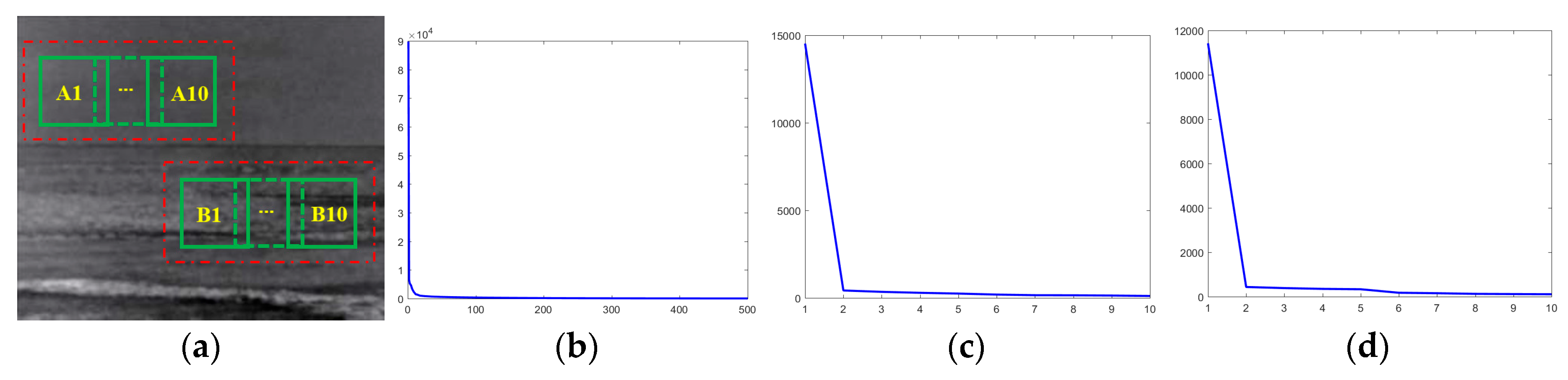
3.1. S1/2N-Induced Low-Rank Model

In order to overcome the limitations of the traditional nuclear norm measurement, nonconvex low-rank regularizers have attracted much attentions in recent years. Schatten p (0 < p < 1)-norm (SpN), which is defined as lp (0 < p < 1) norm of the singular values, is adopted to enforce the low-rank constraint. SpN is defined as:
A S p = ( i = 1 min { m , n } σ i p ) 1 p
where 0 < p < 1, and σ i are the singular values of A.
The nonconvex low-rank regularization induced by SpN can offer better approximation to the original rank function under weaker restricted isometry property than the traditional trace norm [47]. However, when applying SpN to matrix recovery problem, how to select a suitable p and efficiently solve the nonconvex optimization problem induced by SpN is also an interesting problem. Fortunately, a representative role of the index 1/2 in p ( 0 , 1 ) have been demonstrated in Ref. [48]: whenever p [ 1 / 2 , 1 ) , the smaller the p is, the sparser the solutions yield by lp regularization, and when p ( 0 , 1 / 2 ] , the performance of lp regularization has no significant difference. Furthermore, Xu et al. [48] creatively proposed a fast and efficient half-thresholding algorithm for solving the l1/2 regularization problem. With the help of half-thresholding algorithm, Rao et al. [49] solved S1/2N regularization minimization problem quickly and efficiently. In Figure 2, we use both nuclear norm minimization (NNM) and Sp-norm minimization (SpNM) [41], where p takes 0.7, 0.5 and 0.3, to perform low-rank approximation on the matrix of partial adjacent background patch-image (see Figure 2a). Figure 2b presents the deviation of the recovering singular values to the original ones. The singular values obtained by NNM are deviated far from the original ones, clearly exhibiting the over-shrinkage effect of NNM (denoted by green line). Moreover, it is noticed that the difference obtained by SpNM are smaller than NNM. Comparing the results between SpNM when p takes 0.7, 0.5 and 0.3, it is easily observed that the results are in accord with the conclusion drawn by Xu et al. [48]. Nevertheless, the solution process of S0.3NM is so inefficient that it is not suited to real application. Therefore, S1/2N regularization is quite a good candidate for achieving a better approximation.
S1/2N is defined as:
A S 1 / 2 = ( i = 1 min { m , n } σ i 1 / 2 ) 2
With S1/2N relaxation, our developed S1/2NIPI model under the assumption of random noise can be formulated as:
min A , E | | A | | S 1 / 2 1 / 2 + λ | | E | | 1 s . t .   D = A + E + N ,   | | N | | F η
where λ is a global tradeoff between low-rank component and sparse component.

3.2. Reweighted S1/2NIPI Model

However, there are lots of edge clutters, artificial interference objects and pixel-sized noise with high intensity in extremely complex infrared scenes. Relative to the background, these rare structures are easily considered to have similar sparsity to small target under l1 norm measurement. Furthermore, every sparse component element will be treated equally with the usage of a constant sparse parameter λ during the process of l1 norm minimization. It would lead to a dilemma where the weak targets are over-shrunk, resulting missing detection or the rare structures might be divided into target component, causing false alarm. Inspired by reweighted sparse enhancement scheme [38], some methods [33,34] have been proposed to get rid of this predicament by adopting different weight to penalize the different elements. However, although these methods can suppress the rare structures effectively, they ignore the intrinsic geometry of structural targets. From our observation, this is mainly because the traditional way of calculating weights, namely inversely proportional to the real signal values, cannot effectively adjust the degree of weight punishment. Here, a new weight penalty that are different from the traditional weight is defined as follows:
w E , i j k + 1 = q | E i j k | 1 q + ε E
where 0 < q < 1, and ε E is a smoothing parameter to avoid zero division problem.
Here, we will illustrate the effect of the new weight compared with the traditional weight. As shown in Figure 3, we provide the weight curves by the traditional weighted manner and the new weighted manner varying q from 0.1 to 0.9 with interval 0.2. The weight difference between the traditional weight and the new weight with different weight factor q is given to further present the distinct penalty degree under the same values. From the Figure 3c, we can find that the absolute weight difference is very small when q takes 0.1 and 0.3. With the increase of q values, the absolute weight difference increases gradually. It shows that the new weight can better content the punishment degree of different elements by adjusting the q value. Therefore, the proposed method can better deal with different complex scenes and target types with the utility of the new weighted scheme.
Finally, we extend the proposed S1/2NIPI to a reweighted S1/2NIPI (RS1/2NIPI) model for small target detection, which is defined as:
min A , E | | A | | S 1 / 2 1 / 2 + λ | | E | | 1 , W E s . t . D = A + E + N , | | N | | F η
where W E = { w E , i j } are weights for every entry in the target patch-image matrix.

4. Solution of Reweighted S1/2NIPI Model

4.1. Solution of RS1/2NIPI Model

In this section, the proposed reweighted S1/2NIPI model is solved by Alternating Direction Method of Multipliers (ADMM) [46]. It is easy to deduce that the augmented Lagrangian function of problem (8) is:
L ( A , E , Λ ; μ ) = | | A | | S 1 / 2 1 / 2 + λ | | E | | 1 , W E + Λ , D A E + μ 2 | | D A E | | F 2
where μ ( μ > 0 ) is the penalty scalar for the violation of the linear constraint, Λ is the Lagrange multiplier, , denotes the inner product of two matrix. Obviously, the problem (9) is nonconvex, non-smooth and non-Lipschitz. Solving the problem directly seems to be particularly challenging. With the use of ADMM, the Lagrangian function can be effectively tackled by alternative renewal while keeping the current values of the other variables unchanged. Thereby, the problem (9) is decomposed into the following two subproblems, which minimize the variables A k + 1 and E k + 1 separately. The specific update process runs as follows:
A k + 1 = arg min A L ( A , E k , Λ k , μ k ) = arg min A 2 μ k 1 | | A | | S 1 / 2 1 / 2 + | | A ( D E k + Λ k μ k ) | | F 2
E k + 1 = arg min E L ( A k + 1 , E , Λ k , μ k ) = arg min E λ μ k | | E | | 1 , W E + 1 2 | | E ( D A k + 1 + Λ k μ k ) | | F 2
where k denotes as the iteration index.
Solving A k + 1 : The subproblem in Equation (10) is a typical S1/2N regularization minimization problem. Due to the nonconvex relaxation resulted from the S1/2N, the traditional SVT method [50,51] for efficiently solving trace norm minimization can no longer be adopted. Fortunately, Xu et al. [48] have proposed an iterative half-thresholding algorithm for fast solution of L1/2/S1/2 norm regularization. The detailed solution of S1/2N regularization is as the following lemma.
Lemma 1.
[48,52] Let the SVD of W m × n ( m n ) be W = U Σ V T , where Σ = d i a g ( σ 1 , σ 2 , , σ N ) . Suppose that all the singular values are in non-ascending order. For any λ > 0 , the global minimizer X of the following problem
min X m × n | | X W | | F 2 + λ | | X | | S 1 / 2 1 / 2
can be analytically given by:
X = H λ , 1 2 ( W ) = U D i a g ( H λ , 1 2 ( Σ ) ) V T
where H λ , 1 2 ( Σ ) is the half-thresholding operator, which is defined as (14)–(17).
H λ , 1 2 ( Σ ) : = ( h λ , 1 2 ( σ 1 ) , , h λ , 1 2 ( σ N ) ) T
where
h λ , 1 2 ( σ i ) = { f λ , 1 2 ( σ i ) ,   0 , | σ i | > 54 3 4 ( λ ) 2 / 3 o t h e r w i s e
with
f λ , 1 2 ( σ i ) = 2 3 σ i ( 1 + cos ( 2 π 3 2 3 φ λ ( σ i ) ) )
and
φ λ ( σ i ) = arccos ( λ 8 ( | σ i | 3 ) 3 / 2 ) , i = 1 , 2 , , N
In Ref. [48], Xu et al. pointed out that the iterative half-thresholding operator for fast and efficient solution for l1/2 regularization corresponds to the iterative hard-thresholding operator in l0 regularization problem and the iterative soft thresholding operator in l1 regularization problem. The soft-thresholding function [53] is listed as follows:
h λ , 1 ( x ) = { s i g n ( x ) ( | x | λ / 2 ) , 0 , | x | > λ / 2 , x m × n o t h e r w i s e
Inspired by the soft-thresholding algorithm (STA) [53], we design a softening half-thresholding algorithm (SHTA), which is defined as:
H λ , 1 2 S ( Σ ) = ( h λ , 1 2 S ( σ 1 ) , , h λ , 1 2 S ( σ N ) ) T
where
h λ , 1 2 S ( σ i ) = { f λ , 1 2 ( σ i ) f λ , 1 2 ( T ) , 0 , | σ i | > T o t h e r w i s e
and T = 54 3 4 ( λ ) 2 / 3 .
Accordingly, the matrix softening half-thresholding operator is defined as:
H λ , 1 2 S ( W ) : = U D i a g ( H λ , 1 2 S ( Σ ) ) V T
Finally, the subproblem (10) can be solved as:
A k + 1 = arg min A L ( A , E k , Λ k , μ k ) = H 2 μ k 1 , 1 2 S ( D E k + μ k 1 Λ k )
Solving E k + 1 : With the proof of [50], the subproblem in (11) can be solved by the shrinkage operator considered in the following lemma.
Lemma 2.
Given λ > 0 , and X , Y m × n , the global solution of the defined l1-regularized minimization problem:
min X m × n λ | | X | | 1 + 1 2 | | X Y | | F 2
can be approached by element-wise soft-thresholding operator defined as:
S λ ( Y ) = s i g n ( Y i j ) max ( | Y i j | λ , 0 )
Then, the solution of Equation (11) is as follows:
E k + 1 = arg min E L ( A k + 1 , E , Λ k , μ k ) = S λ μ k 1 W E ( D A k + 1 + μ k 1 Λ k )
The solution of the reweighted S1/2NIPI model (RS1/2NIPI) is summarized in Algorithm 1.
Algorithm 1 The solution of RS1/2NIPI model using ADMM
1: Input: Original patch-image D, parameter λ ;
2: Initialize: A 0 = E 0 = 0 ; Λ 0 = D max ( | | D | | 2 ; M | | v e c ( D ) | | inf ) ; μ 0 = 1.25 | | D | | 2 ; μ max = 10 7 ; W 0 = I m × n ; ε E = 0.01 ; k = 0;
3: While not converged do
4: Solving A k + 1 by
5:  A k + 1 = H 2 μ k 1 , 1 2 S ( D E k + μ k 1 Λ k )
6: Solving E k + 1 by
7:  E k + 1 = S λ μ k 1 W E ( D A k + 1 + μ k 1 Λ k )
8: Update Λ
9:  Λ k + 1 = Λ k + μ k ( D A k + 1 E k + 1 )
10: Update μ k + 1 , w E , i j k + 1
11:  μ k + 1 = min { β μ k , μ max }
12:  w E , i j k + 1 = q | E i j k | 1 q + ε E
13: Check the convergence conditions
14:  | | D A k + 1 E k + 1 | | F | | D | | F < ε   o r   | | E k + 1 | | 0 = | | E k | | 0
15: Update k
16: k = k + 1
17: end while
18: Output: A, E;

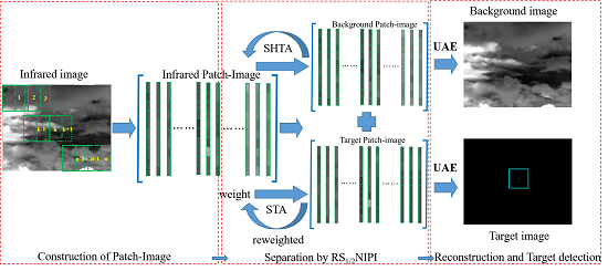
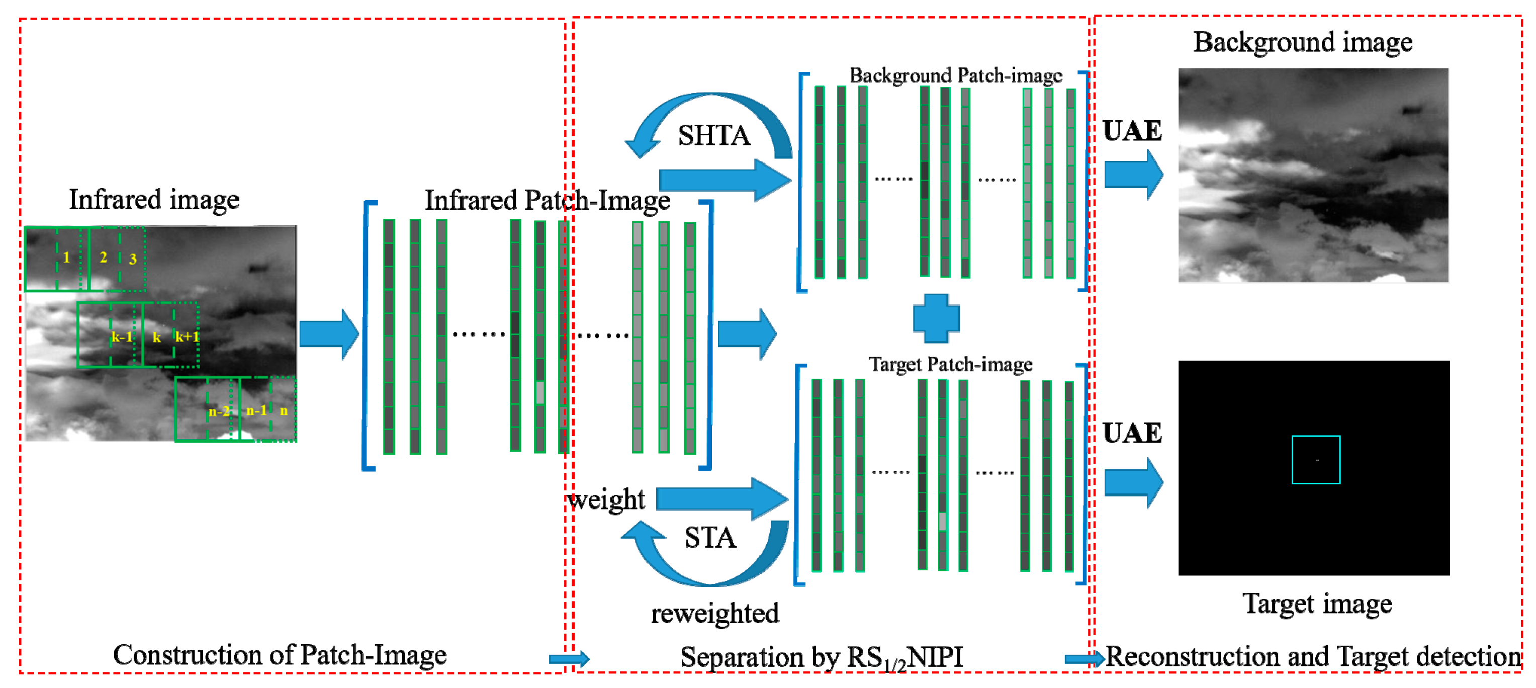
4.2. Whole Detection Procedure of the Proposed Model

To intuitively display the proposed model for detecting infrared small target, its schematic is given in Figure 4.
The detailed procedure are as follows:
(1)
By using the same local patch construction as IPI model, the original infrared image fD is decomposed into the infrared patch-image D.
(2)
Algorithm 1 is employed to perform the target-background separation.
(3)
By applying the uniform average of estimators (UAE) reprojection scheme, the background image fA and target image fE are reconstructed from the background patch-image A and target patch-image E.
(4)
The final target is separated by an adaptive threshold, which is determined by:
T u p = max ( υ min , ρ + c σ )
where ρ and σ are the mean value and standard deviation of the target image fE, respectively. c and υ min are constants determined experientially.

5. Experimental Analysis

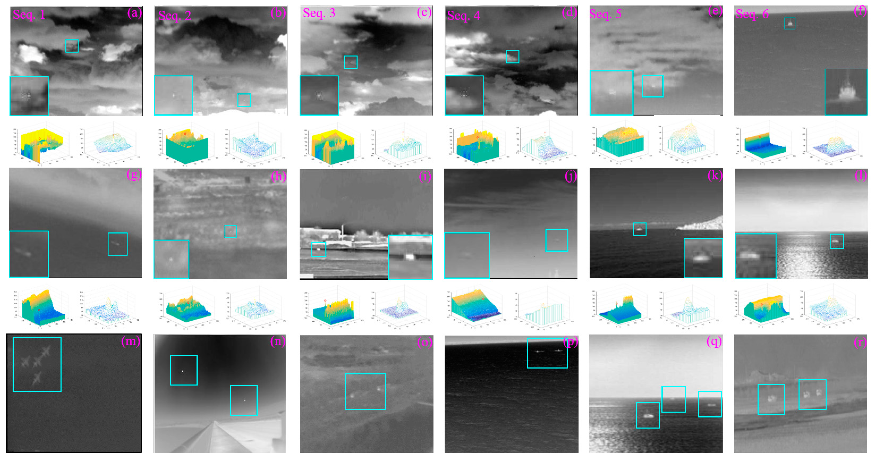
5.1. Datasets and Evaluation Criterions

Datasets: In order to verify the reliability and effectiveness of the proposed method, we conduct extensive experiments on real infrared images with various scenes including aerial, maritime, sky-cloud and terrain scenes. These scenes vary from uniform background with single salient target to complex background with heavy clutters and multiple dim targets, as shown in Figure 5. In Figure 5a–l, each scene contains one target, which is labeled with cyan box and enlarged to facilitate observation for extreme weak one. The 3-D projections of the global image and the demarcated area are placed below the image in order to present the complexity of the whole and local environment. In Figure 5m–r, multiple targets are contained in every scene and labeled with cyan box as well. They have different size and styles, such as missile or plane in sky-cloud background, cruise or speedboat in maritime scene and vehicle in terrain situation. Among these scenes, Figure 5a–f are real infrared sequences. The detailed information of all datasets is listed in Table 1.
Evaluation criterions: Here, four commonly used metrics are introduced for performance comparison quantitatively, including the signal-to-clutter ratio gain (GSCR), background suppression factor (BSF), local signal-to-noise ratio gain (GLSNR) and receiver operating characteristic (ROC). The GSCR, BSF and GLSNR are calculated based on the neighborhood region around the target, as illustrated in Figure 6. Suppose that the target size is a × b , and d is the neighborhood width, which takes d = 20 in our paper.
As a measurement of target saliency, SCR is frequently used to represent the difficult level of target detection, which is defined as:
S C R = | μ t μ b | σ b
where μ t and μ b are the average grayscale of the target area and its nearby region, respectively. σ b corresponds to the standard deviation of the neighborhood region. Then, the SCR gain (GSCR) is defined as the ratio of the SCR before and after processing, which is written as:
G S C R = S C R o u t S C R i n
where SCRin and SCRout are the SCR values before and after target detection separately. The higher the GSCR is, the better the target enhancement will be. BSF is usually employed to measure the background suppression ability of detection methods, which is defined as:
B S F = σ i n σ o u t
where σ i n and σ o u t are the standard deviation of background neighborhood in original image and the suppressed image. Besides GSCR and BSF, GLSNR emphasizes the local signal-to-noise ratio gain of target neighborhood before and after background suppression, which is defined as:
G L S N R = L S N R o u t L S N R i n
where L S N R i n and L S N R o u t denote the L S N R values of the original and processed image, respectively. L S N R is defined as L S N R = I T / I B , where I T and I B are the maximum pixel values of the target and its neighborhood, respectively. In general, the larger the above three indexes are, the superior the detection performance is.
Despite the above three metrics, the detection probability Pd and false-alarm ratio Fa are the most important evaluating indicators for evaluating the target detection performance, which are defined as:
P d = number   of   true   detections number   of   actual   targets
F a = number   of   false   detections number   of   images
When owning both high detection probability and low false alarm rate at the same time, the method is considered as a good detector. The receiver operating characteristic (ROC) curve represents the tradeoff between the true and false detections. The steeper and higher the curve is, the more robustness the detection performance is.

5.2. The Performance Analysis of the Proposed Model

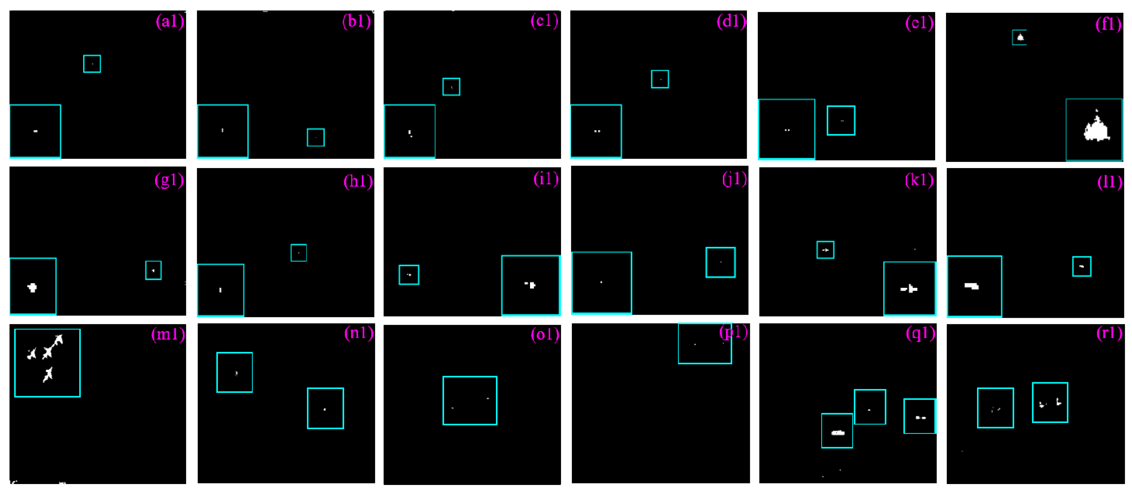
5.2.1. Evaluation on Single and Multiple Targets Images

From the Figure 5, it is easily observed that the datasets include diverse background with different interferences, such as noise bright spots, manmade artifacts, heavy cloudy clutters and sea glints. These disturbances lead to great difficulties or challenges in the task of small target detection. Therefore, the detection performance on these datasets are more cogent than the desirable results on relatively simple scenes. Figure 7 displays the detection results of the proposed method. For convenient observation of the detection results, the target area is enlarged in single target results. In the Figure 7, it is obviously seen that the proposed method not only eliminate background disturbances and extract the small target, but also basically maintain the target completeness (see Figure 7(f1,m1)).

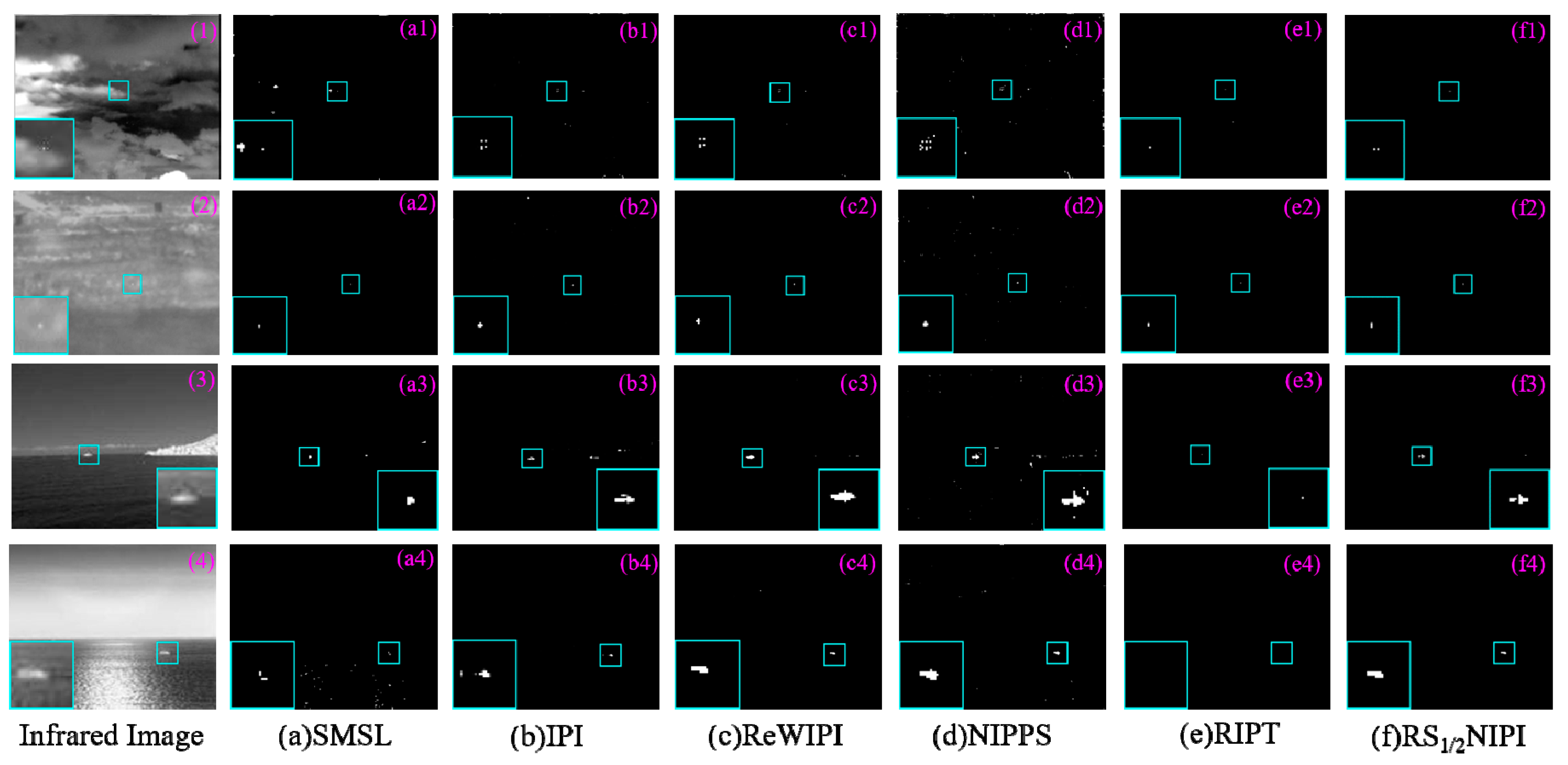
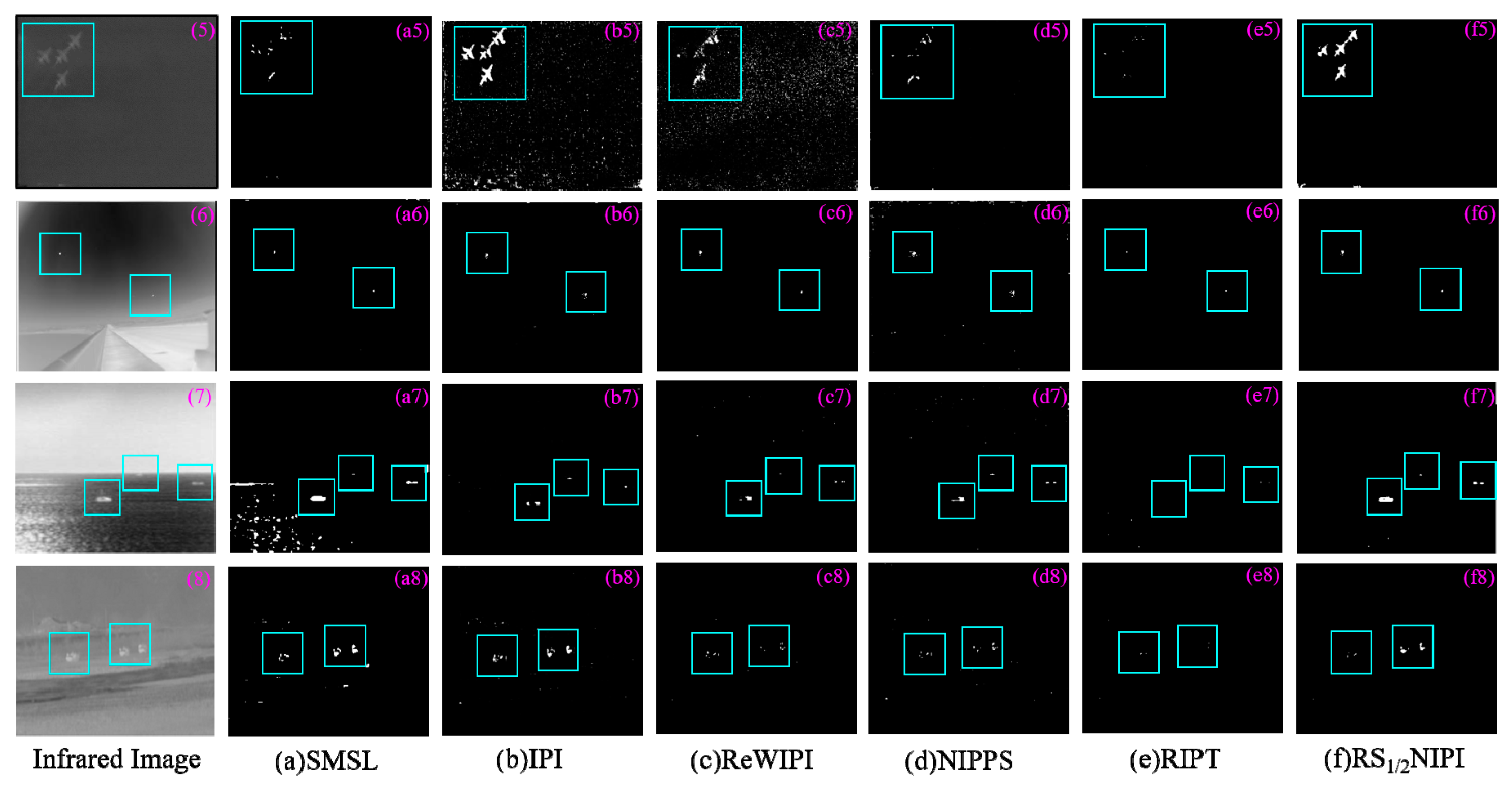
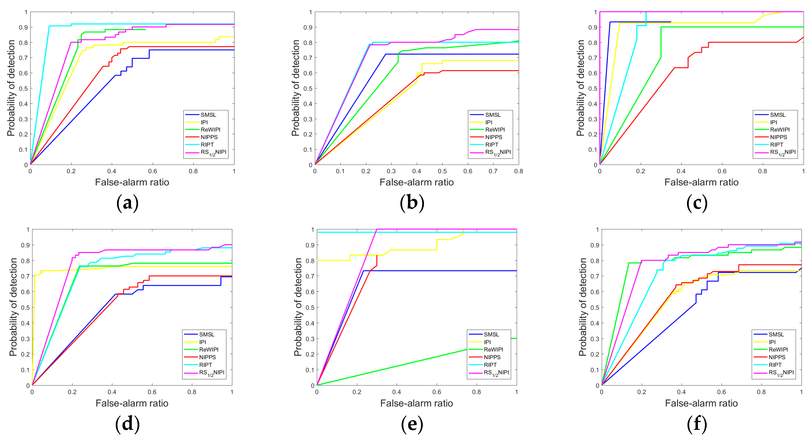
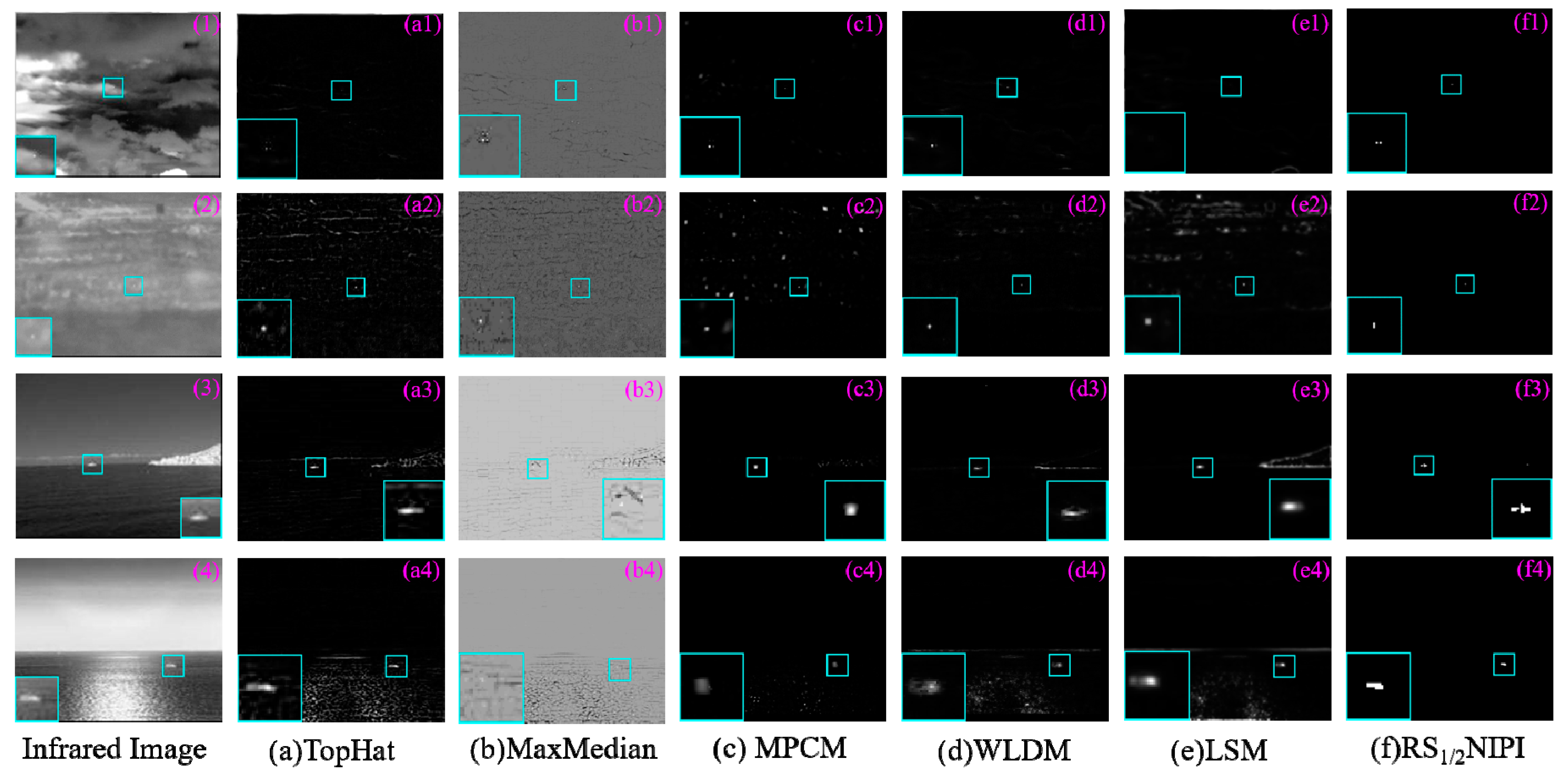
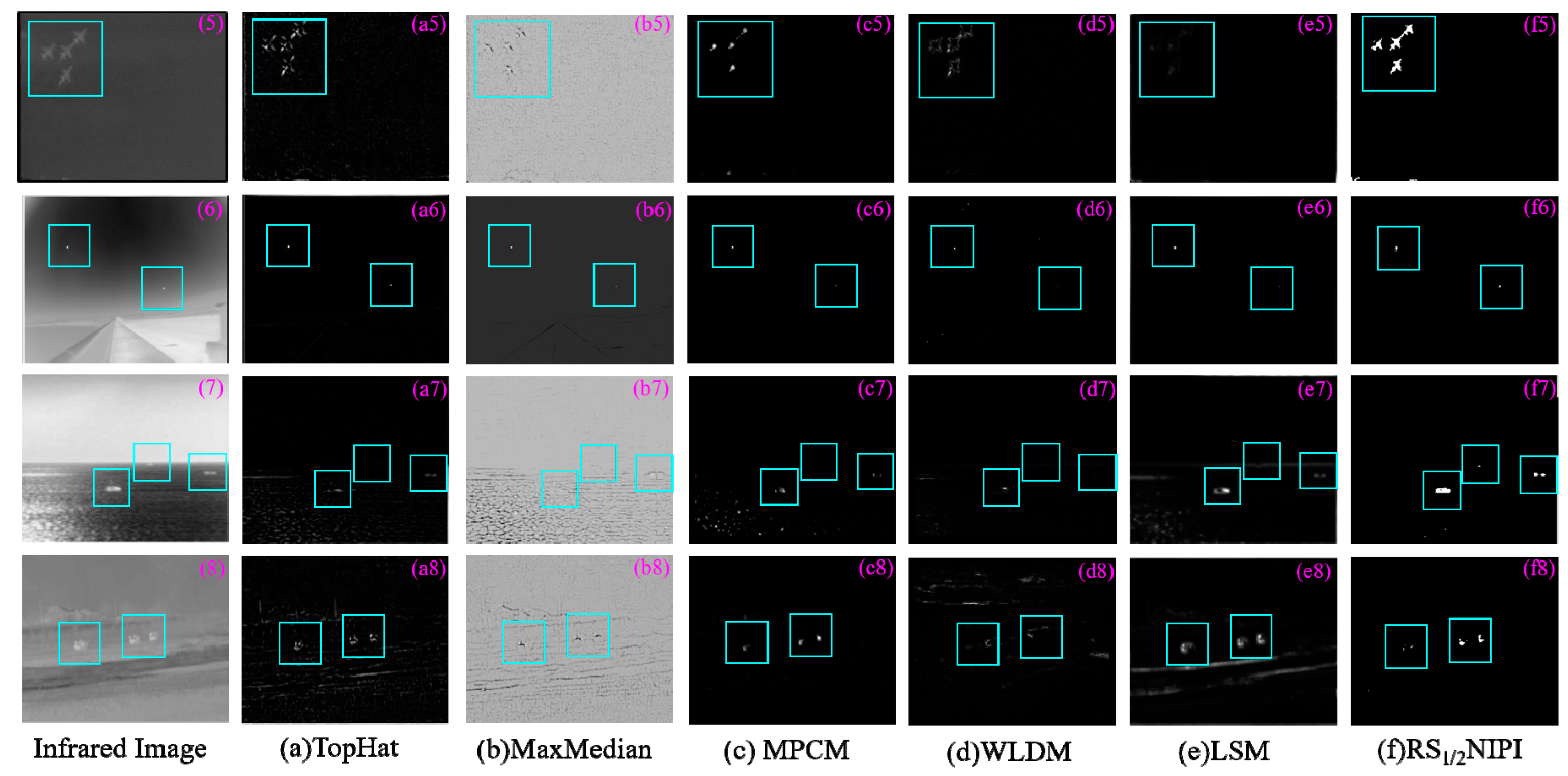
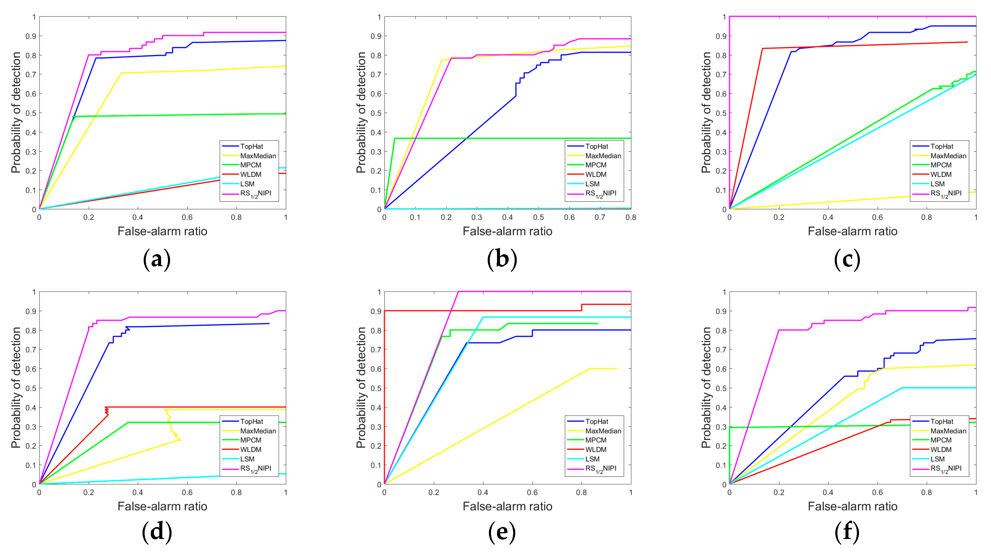
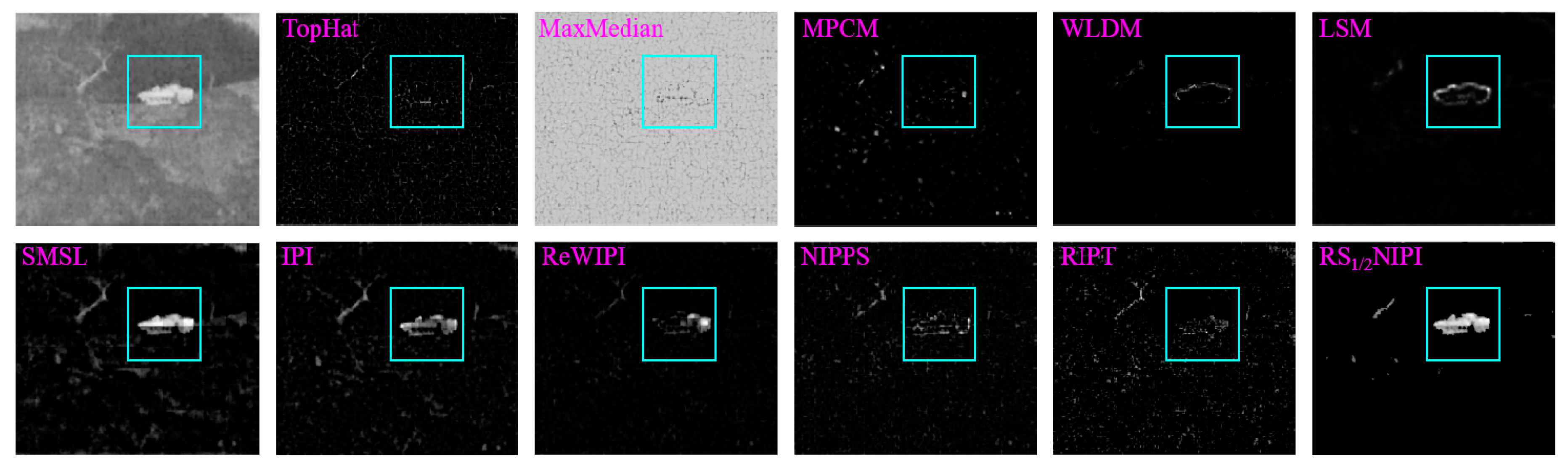
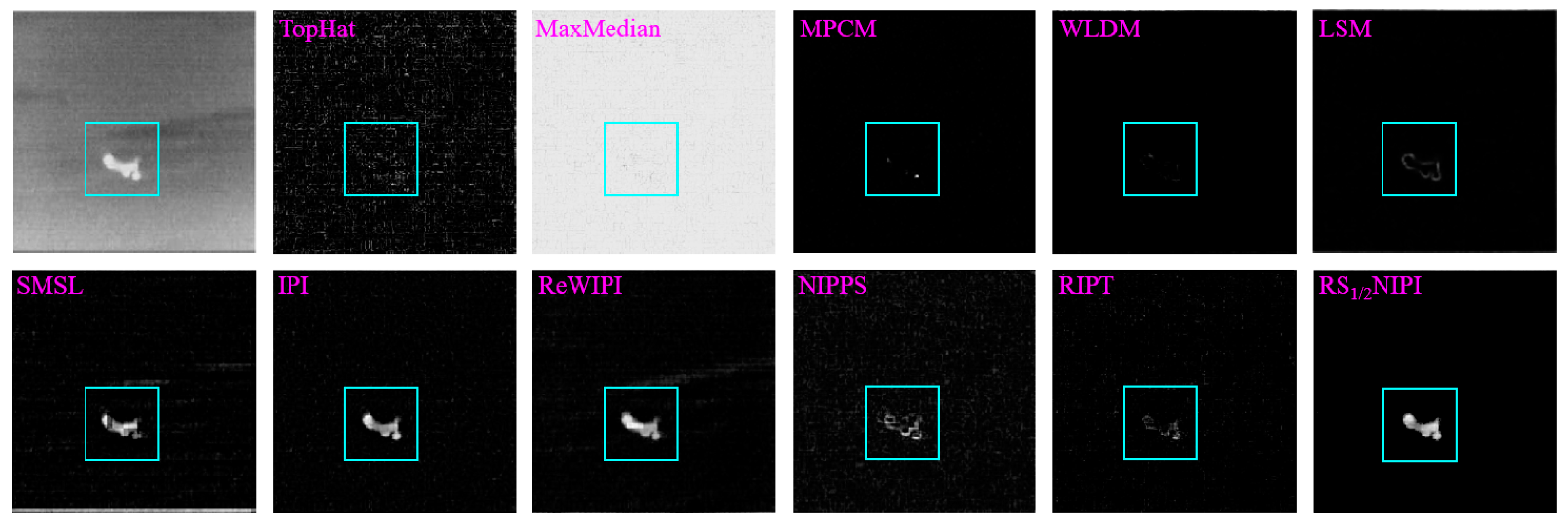
5.2.2. Comparison to the State-of-the-Art Methods

A full investigation for evaluating the performance of the proposed method are given in comparisons with ten state-of-the-arts with respect to both quantitatively and qualitatively.
The compared nonlocal correlation-based models include Stable Multi-subspace Learning (SMSL) [36], Infrared Patch-Image model (IPI) [32], Reweight Infrared Patch-Image model (ReWIPI) [33], Non-negative Infrared Patch-Image based on Partial Sum minimization of singular values (NIPPS) [42], Reweight Infrared Patch-Tensor model (RIPT) [34]. The objective functions and parameter settings for each model are listed in Table 2. Moreover, the including parameters are tuned to obtain optimal results.
The focus of the low-rank recovery-based methods is put on how to separate small targets from the various backgrounds with as low false and/or missing alarm as possible. To validate the separated performance of the proposed method, the tests on images with the single and multiple targets are conducted by the comparative methods and the proposed method. The separated results performed on the scenes with single and multiple targets are shown in Figure 8 and Figure 9, respectively. In Figure 8, it is notice that all targets can be separated by the proposed and comparative methods without missing detection in the single-target images. However, many nontarget sparse residuals are remained in the separated results processed by SMSL, IPI and NIPPS, which would cause false alarm. In contrast, ReWIPI, RIPT and the proposed model achieve the better separated results with low false and missing detection. For images with multiple targets, Figure 9 shows the multiple targets results separated from complex background via the comparative and proposed methods. From the figures, one can see that SMSL, IPI, ReWIPI and NIPPS suffer from incorrect separation of the strong edge or sparse point into the target images and the incompleteness of the targets. In addition, even though RIPT suppresses all background clutters very well, it fails in detecting the targets with sparse structure because of its over-emphasizing on the sparsity of target. By contrast, whether in the single-target or the multi-targets results, our proposed method can pop out the targets with low false alarm rate, and maintain its completeness successfully. Therefore, the conclusion drawn from Figure 8 and Figure 9 is that the proposed method achieves the superiority over other comparative methods for different target size, number and background types.
Furthermore, The ROC curves obtained by the proposed and comparative methods for Sequences 1–6 are provided in Figure 10. Obviously, the ROC curves plotted by the proposed method climb higher and faster than other competitive methods and achieve the highest Pd among them. This demonstrates that the proposed method outperforms the compared low-rank recovery-based methods in terms of the tradeoff between Pd and Fa. In Sequence 1, although the Pd of the proposed method are lower than RIPT when Fa < 0.66, they will rise to the same level as RIPT as Fa increases. The proposed method arrives the highest Pd rapidly in other sequences among all baseline methods. In addition, the proposed method has great advantages compared with RIPT under the emergence of structurally sparse target, as illustrated in latter section.
Furthermore, the GSCR, BSF and GLSNR of all methods for Figure 5a–e are shown in Table 3. For each indicator, a higher value denotes the better performance. For the low-rank modeling-based methods, Inf, namely infinity, is often appearing, but it just means that the target neighboring region is completely suppressed. In Table 3, for the three indexes, many methods have obtained Inf. Nevertheless, we should understand clearly that this merely reflects the suppression effect in a local area rather than the whole.
The filtering and saliency-based methods concentrate on how to pop out or enhance targets and suppress backgrounds as much as possible. In the following experiments, the comparative methods contain two classical filtering methods, namely TopHat [14] and MaxMedian [9], and three state-of-the-art saliency-based methods, namely Weighted Local Difference Measure (WLDM) [21], Multiscale Patch-based Contrast Measure (MPCM) [22], Local Saliency Map (LSM) [20]. We list the five experimental methods and their detailed parameter settings in Table 4.
The results obtained by these comparative methods handled on the representative single and multiple targets images are shown in Figure 11 and Figure 12. In Figure 11, it is evident that the performance of the methods based on saliency is much better than the two classical filtering methods. The MaxMedian filter does enhance the small target, but the heavy clutters or strong edges are also enhanced at the same time. For TopHat, when the selected structure element is consistent with the actual target size, it can enhance the target area very well, as shown in Figure 11(a1–a4). However, TopHat does not suppress the background clutters very well. Although all targets are successfully detected by WLDM, MPCM and LSM, there are many salient sparse residuals in the detecting images. It is because that when facing dimmer target and strong clutter, the local difference/contrast measure fails to depict the salient non-target components completely. For the multiple targets images, the detection results achieved by the comparative methods either contain a large of strong clutters or miss some targets, because of their poor ability to detect structural targets and suppress backgrounds, as shown in Figure 12.
In Figure 13, the ROC curves of Sequences 1–6 implemented by TopHat, MaxMedian, WLDM, MPCM, LSM are provided. The curves indicate that our proposed method work better than other competitive methods. However, it is interesting to note that the TopHat achieves an impressive detection performance in tested sequences. The main reason is that the selected structure element matches the tested sequences with slowly varying background very well, which is suited to filtering-based methods. Moreover, the detection performance of saliency-based methods changes greatly. The major reason lies in that for different sequences, there are various strong disturbances that have higher contrast than targets in local background, causing high false alarm. The GSCR, BSF and GLSNR of the filtering and saliency-based methods are summarized in Table 5. It shows that the proposed method outperforms the comparative methods in term of the target and background extraction for various types of complex background.

5.2.3. Evaluation on Structurally Sparse Target Scenes

Figure 14, Figure 15 and Figure 16 show three example of structurally sparse target scenes and the corresponding target-background separated results implemented by the different tested methods. In view of the background types of the three representative raw scenes, they contain sky-terrain, cloudy-sky and sea-land background. It can be found that these representative scenes contain heavy noise, bright interference spots, strong cloudy clutters and manmade buildings, which make the complete target detection more challenging. Observing the figures, we can find that the filtering methods (TopHat and MaxMedian) perform worse on edge clutter suppression and target detection. This is mainly because these structural targets are spatially consistent to some extent and will be filtered out as backgrounds. Although the small targets can be detected by saliency-based methods, the details of the target are missing. From the results processed by low-rank recovery-based methods, one can see that they achieve better performance than saliency-based and filtering methods in terms of detection probability and integrity. Compared with other methods, the proposed method achieves a good balance between background clutter suppression and target integrity preservation, that is, it can detect small targets completely with little background clutter residuals.

5.3. Discussion

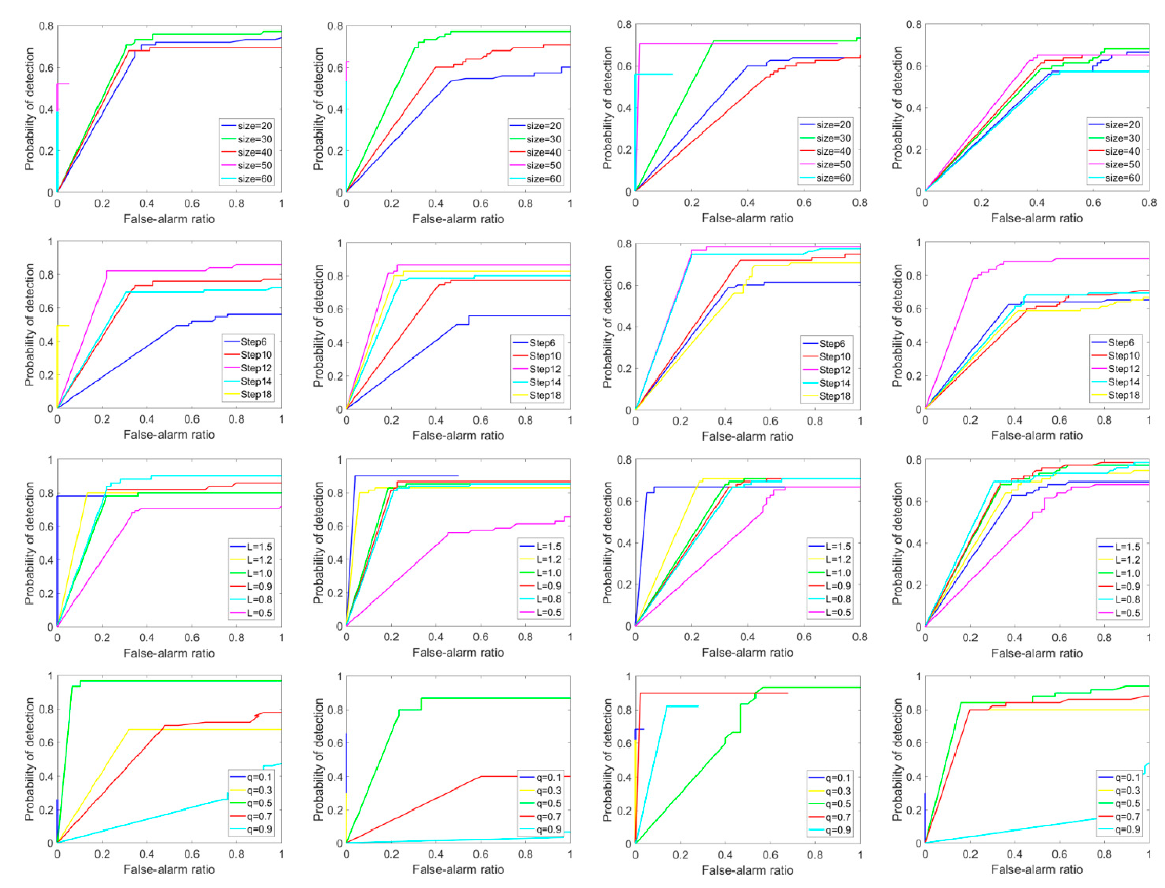
5.3.1. The Effect of Different Parameters

In our proposed model, several critical parameters should be selected reasonably, including patch size, sliding step, sparse penalty λ and weight factor q. Therefore, we conduct several experiments on Sequences 1–4 to analyze the effects of the above four parameters. The ROC curves of detection results for the different parameters are provided in Figure 17.
For patch size, its different values do have an impact on the complexity and detection performance in the proposed model. Taking account of the computational complexity, the structural sparsity of target and the nonlocal correlation of background together, we set the patch size by varying from 20 to 60 with ten intervals to discuss the effects of the patch size. The first row of Figure 17 shows the ROC curves of the detection results obtained by our proposed method with different patch sizes. It can be observed that the choice of patch size 30 × 30 can achieve the best result under the sequential cases. Moreover, we set patch size to 50 × 50 on the single frame image.
To analyze the effects of the sliding step, with the patch size 30 × 30 invariable, we set the sliding step as 6, 10, 12, 14, 18, respectively, and then test the proposed method. The experimental results are presented in the second row of Figure 17. From the figures, we can find that for all test sequences, when the sliding step is taken as 12, the proposed model can achieve the optimal performance.
For the sparse penalty λ , it balances the influence between low-rank component and sparse component. Therefore, it is meaningful to investigate the parameter for verifying the detection performance of our proposed model. In our test, the L / max ( m , n ) is a substitute for directly varying the sparse penalty λ . We set the L as 0.5, 0.8, 0.9, 1.0, 1.2, 1.5, respectively, whose ROC curves are shown in the third row of Figure 17. In the figures, it can be easily noticed that when L is set in the interval [0.8 1.2], the proposed model performs better. Nevertheless, when we encounter the scenes that is different from our test datasets, an optimal sparse penalty λ should be selected experimentally.
For the weight factor q, it controls the sparse weight’s suppression degree to salient outliers. We vary q from 0.1 to 0.9 with 0.2 interval to verify its influence on detection performance and give the ROC curves in the fourth row of Figure 17. From the illustration of ROC curves, we notice that if the value of q is too large or too small, the robustness of the algorithm will degrade. For example, when q = 0.1, the proposed method achieves low false alarm rate but obtains lower detection probability. It is because the dim target appears in many frames of the tested sequences and a smaller q would suppress clutter residuals but easily over-punish weak target, resulting in missing detection. On the contrary, a larger q might preserve the weak target, but it also retains some nontarget points, leading to increase in false alarm. As shown in ROC curves with different weight factor, q = 0.5 seems a better choice because it realizes the best detection effectiveness and robustness.

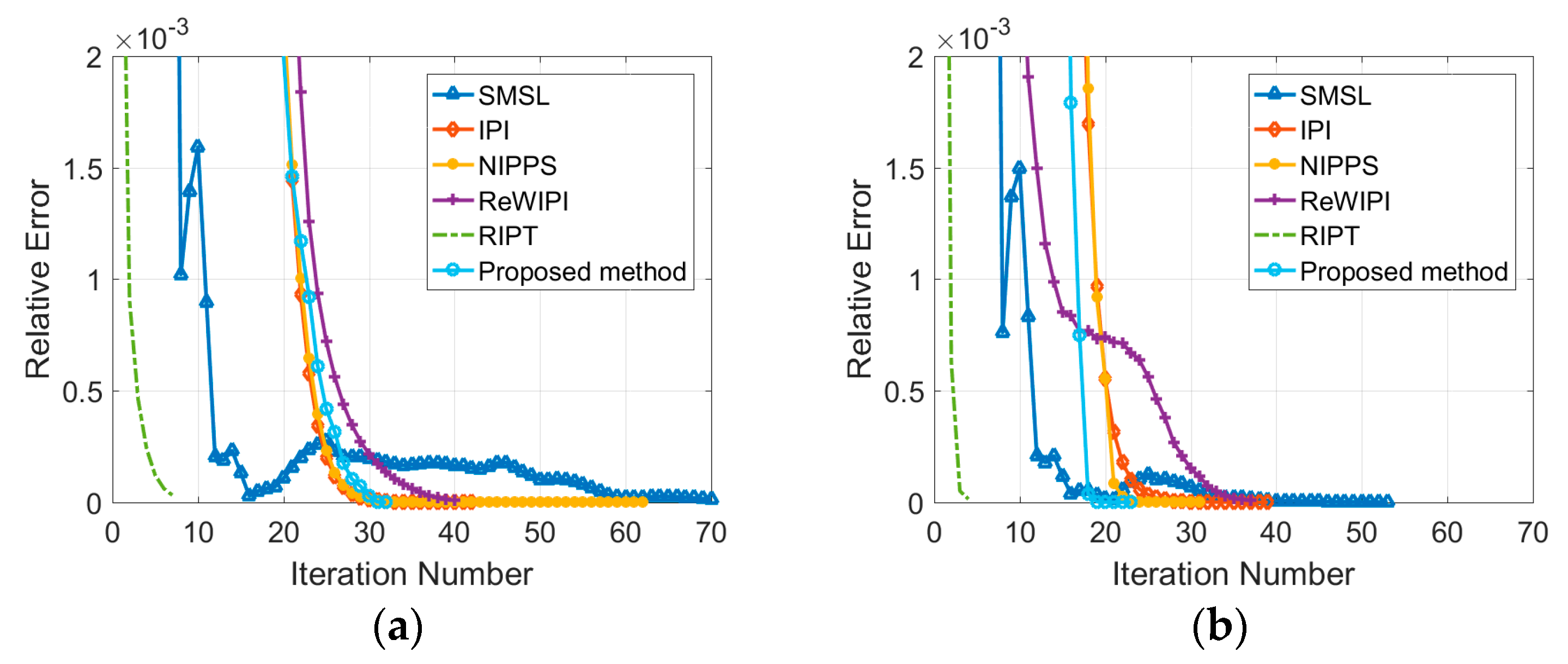
5.3.2. Convergence and Time-Consuming Analysis

All tests are performed on a personal computer with an Intel(R) i5-8700 CPU (3.40 GHz) and 8G RAM using MATLAB 2016b. The effective solution of the proposed algorithm can be obtained by ADMM, which has been proved a O ( 1 / k ) convergence [54]. The convergence curves of methods based on low-rank recovery are provided in Figure 18. In order to make a fair comparison, we take the error tolerance as 10−7 and set the relative error as 0.002 for convenient observation. Form the figures, it is easily noticed that the convergence rate of RIPT is the fastest. It is because counting the number of elements in sparse component is served as an additional stopping criterion, which avoids excessive iteration. Although the proposed algorithm is slower than RIPT, it converges faster than other methods. It shows that the softening half-thresholding operator does not slow down the convergence rate of the proposed method. In SMSL, it is solved by the Accelerated Proximal Gradient (APG) algorithm, resulting slow convergence rate. Here, we exploit ADMM to solve IPI model, which gives a more accurate solution and is at least five times faster than its original APG version. However, the time consumption of an algorithm is determined based on not only the convergence rate, but also other factors, such as computational complexity, image size and optimization algorithm, and so on.
To better analyze the timeliness of the proposed method, the average consuming time of all methods in per frame of the Sequence 1–6 is shown in Table 6. Clearly, the filtering and saliency-based methods are faster than the low-rank recovery-based methods. This is because the filtering and saliency-based methods merely run on the pixel level, which can be viewed as a rearrangement of pixels in original image and no adds additional computational complexity. For low-rank recovery-based methods, SVD step in every iteration occupies most of the total time consuming. However, the methods based on filtering and saliency have poor detection performance when encountering complex scenes. Therefore, the low-rank recovery methods are cost-effective in terms of reliability and robustness. Among the low-rank recovery-based methods, the proposed method runs faster than IPI, ReWIPI and NIPPS, but slower than SMLS and RIPT. The main reason lies in that SMSL utilizes the block coordinate descent method to avoid the SVD in every iteration, which speeds up the optimization process and RIPT employs both local structure and sparsity enhancement weight to reduce the iteration number. In our proposed model, the iterative softening half-thresholding method may increase the computational burden to some extent. But the proposed model can avoid the redundant iteration by using the same additional stopping criterion as RIPT, accelerating the convergence rate. Considering that the proposed method has much better performance against various complex background and target types, and the advanced acceleration scheme based on GPU or FPGA could reduce time-consuming differences to a negligible extent, we conclude that the proposed method is more desirable.

6. Algorithm Advantage and Limitation Analysis

Many efforts have been concentrated on improving the detection performance in infrared small target search and tracking community over the past few decades. Designing a detection method concurrently possessing timeliness, strong robustness and superior performance is always an open problem. The real-time detection can be achieved by the filtering and saliency-based methods under gray-level spatial or saliency-induced feature spatial. However, they have poor detection performance and robustness when encountering complex scenes. In addition, the intrinsic structure of whole background and target region are all ignored in these methods, causing the incompleteness of structural target or even missing target in detection results. The low-rank recovery-based methods have superior detection performance and stability than the filtering and saliency-based methods. It attributes the success to the better matching of the assumption of the nonlocal correlation of background and the sparsity of target to general scenarios. Nevertheless, the performance of the low-rank recovery-based methods might degrade seriously when facing extremely complicate scenes with structural small targets. It is mainly because rare structures in these backgrounds would have the similar sparsity to the small target but structural target might present nonlocal correlation under the IPI model. Some methods, such as ReWIPI, NIPPS, SMSL, NRAM and RIPT have been proposed to attempt to address these issues. But some of them have high computational cost, reducing real-time performance.
In the proposed method, S1/2N is used to constrain the background patch-image, which can punish the smaller singular values precisely, preserving the rare structure components in background as much as possible. It helps to better restore the background in complex scenes. Besides, a new weight with adaptive penalty can suppress the target-like components, which might have similar thermal intensity to the real target, by tailoring the weight factor q. Finally, under the optimization framework of ADMM, the subproblem of S1/2N minimization can be solved by the designing soft half-threshold operator and an additional stopping criterion is used to avoid the excessive iteration, ensuring the balance among the detection performance and computational cost. The above advantages make the proposed method achieve superiority in the detection of small target with different types and sizes in the diverse complex scenes. However, two limitations still exist in the proposed method. First, when there is salient interference with higher intensity or contrast than target in background, the proposed method may not suppress it. Second, a small amount of clutter interference is leaved in the detection results of structural target in order to retain the integrity of target in some scenes. These issues can be solved by properly integrating the global and local prior of background and target in future work. As a whole, the proposed method is more desirable compared with ten state-of-the-art methods in terms of detection performance, robustness and computational cost.

7. Conclusions

In this work, we have presented a novel nonconvex low-rank regularization-based method for infrared dim and small target detection in complex scenes. First, Schatten 1/2 quasi-norm (S1/2N), is a substitute for the trace nuclear norm. It achieves better approximation for the sparse-regularized low-rank function, exactly recovering the background patch-image. Then, an adaptive weight is applied to suppress the salient sparse outliers. Accordingly, the target-background distinguishing task is converted to low-rank recovery problem with S1/2N regularization, which is efficiently solved by ADMM. Moreover, the softening half-thresholding operator, instead of the original half-thresholding operator, is used to solve S1/2N minimization subproblem. Extensive evaluations on different real scenes of both single target and multiple targets reveal that the proposed method exhibits higher accuracy and reliability than the state-of-the-art methods in terms of qualitative and quantitative. Taking into account the application prospects of the proposed method, how to adaptively choose the tradeoff parameter λ to further improve the flexibility for the target size and meet the real-time requirements simultaneously is considered as the future work.

Author Contributions

F.Z. conceived the original idea, conducted the experiments and wrote the manuscript. Y.D. helped with data collection. Y.D., P.W. and Y.W. contributed to the writing, content and revised the manuscript.

Funding

This work was supported in part by the National Nature Science Foundation of China under Grant 61573183; 61801211 and the Open Project Program of the National Laboratory of Pattern Recognition (NLPR) under Grant 201900029.

Acknowledgments

The authors would like to thank the editor and anonymous reviewers for their help comments and suggestions and thank Chengqiang Gao and Xiaoyang Wang providing images and the codes for comparison.

Conflicts of Interest

The authors declare that there is no conflict of interesting.

References

  1. Bai, X.Z.; Chen, Z.; Zhang, Y.; Liu, Z.; Lu, Y. Infrared ship target segmentation based on spatial information improved FCM. IEEE Trans. Cybern. 2016, 46, 3259–3271. [Google Scholar] [CrossRef] [PubMed]
  2. Gao, J.L.; Wen, C.L.; Liu, M.Q. Robust small target co-detection from airborne infrared image sequences. Sensors 2017, 17, 2242. [Google Scholar] [CrossRef]
  3. Deng, H.; Sun, X.P.; Zhou, X. A multiscale fuzzy metric for detecting small infrared targets against chaotic cloudy/sea-sky backgrounds. IEEE Trans. Cybern. 2018, 99, 1–14. [Google Scholar] [CrossRef] [PubMed]
  4. Bai, X.Z.; Bi, Y.G. Derivative entropy-based contrast measure for infrared small-target detection. IEEE Trans. Geosci. Remote Sens. 2018, 99, 1–15. [Google Scholar] [CrossRef]
  5. Gao, C.Q.; Wang, L.; Xiao, Y.X.; Zhao, Q.; Meng, D.Y. Infrared small-dim target detection based on Markov random field guided noise modeling. Pattern Recogn. 2018, 76, 463–475. [Google Scholar] [CrossRef]
  6. Dong, L.L.; Wang, B.; Ming, Z.; Xu, W.H. Robust infrared maritime target detection based on visual attention and spatiotemporal filtering. IEEE Trans. Geosci. Remote Sens. 2017, 99, 1–14. [Google Scholar] [CrossRef]
  7. Chang, H.; Yuan, L.; Ramakant, N. Multiple target tracking by learning-based hierarchical association of detection responses. IEEE Trans. Pattern Anal. 2013, 35, 898–910. [Google Scholar]
  8. Kim, S.; Lee, J. Scale Invariant small target detection by optimizing signal-to-clutter ratio in heterogeneous background for infrared search and track. Pattern Recogn. 2012, 45, 393–406. [Google Scholar] [CrossRef]
  9. Deshpande, S.D.; Meng, H.E.; Ronda, V.; Chan, P. Max-mean and Max-median filters for detection of small-targets. Proc. SPIE Int. Soc. Opt. Eng. 1999, 3809, 74–83. [Google Scholar]
  10. Hadhoud, M.M.; Thomas, D.W. The Two-Dimensional Adaptive LMS (TDLMS) algorithm. IEEE Trans. Circuits Syst. 1988, 35, 485–494. [Google Scholar] [CrossRef]
  11. Baem, T.W.; Zhang, F.; Kweon, I.S. Edge directional 2D LMS filter for infrared small target detection. Infrared Phys. Technol. 2012, 55, 137–145. [Google Scholar]
  12. Zhao, Y.; Pan, H.; Du, C.; Peng, Y.; Zheng, Y. Bilateral two dimensional least mean square filter for infrared small target detection. Infrared Phys. Technol. 2014, 65, 17–23. [Google Scholar] [CrossRef]
  13. Zeng, M.; Li, J.; Peng, Z. The design of top-hat morphological filter and application to infrared target detection. Infrared Phys. Technol. 2006, 48, 67–76. [Google Scholar] [CrossRef]
  14. Bai, X.Z.; Zhou, F.G. Analysis of new top-hat transformation and the application for infrared dim small target detection. Pattern Recogn. 2010, 43, 2145–2156. [Google Scholar] [CrossRef]
  15. Peng, L.B.; Zhang, T.F.; Liu, Y.H.; Li, M.H.; Peng, Z.M. Infrared dim target detection using shearlet’s kurtosis maximization under non-uniform background. Symmetry 2019, 11, 732. [Google Scholar] [CrossRef]
  16. Chen, C.L.; Li, H.; Wei, Y.T.; Xia, T.; Tang, Y.Y. A local contrast method for small infrared target detection. IEEE Trans. Geosci. Remote Sens. 2013, 52, 574–581. [Google Scholar] [CrossRef]
  17. Han, J.H.; Ma, Y.; Zhou, B.; Fan, F.; Liang, K.; Fang, Y. A robust infrared small target detection algorithm based on human visual system. IEEE Geosci. Remote Sens. 2014, 11, 2168–2172. [Google Scholar]
  18. Qin, Y.; Li, B. Effective infrared small target detection utilizing a novel local contrast method. IEEE Geosci. Remote Sens. 2016, 99, 1–5. [Google Scholar] [CrossRef]
  19. Han, J.H.; Liang, K.; Zhou, B.; Zhu, X.Y.; Zhao, J.; Zhao, L.L. Infrared small target detection utilizing the multiscale relative local contrast measure. IEEE Geosci. Remote Sens. 2018, 15, 612–616. [Google Scholar] [CrossRef]
  20. Chen, Y.W.; Xin, Y.H. An efficient infrared small target detection method based on visual contrast mechanism. IEEE Geosci. Remote Sens. 2016, 13, 962–966. [Google Scholar] [CrossRef]
  21. Deng, H.; Sun, X.P.; Liu, M.L.; Ye, C.H.; Zhou, X. Small infrared target detection based on weighted local difference measure. IEEE Trans. Geosci. Remote Sens. 2016, 54, 4204–4214. [Google Scholar] [CrossRef]
  22. Wei, Y.T.; You, X.G.; Li, H. Multiscale patch-based contrast measure for small infrared target detection. Pattern Recogn. 2016, 58, 216–226. [Google Scholar] [CrossRef]
  23. Nie, J.Y.; Qu, S.C.; Wei, Y.T.; Zhang, L.M.; Deng, L.Z. An infrared small target detection method based on multiscale local homogeneity measure. Infrared Phys. Technol. 2018, 90, 186–194. [Google Scholar] [CrossRef]
  24. Wei, Y.T.; You, X.G.; Deng, H. Small infrared target detection based on image patch ordering. Int. J. Wavelets. Multi. 2016, 14, 1640007. [Google Scholar] [CrossRef]
  25. Deng, H.; Sun, X.; Liu, M.; Ye, C.; Zhou, X. Entropy-based window selection for detecting dim and small infrared targets. Pattern Recogn. 2017, 61, 66–77. [Google Scholar] [CrossRef]
  26. Deng, H.; Sun, X.P.; Liu, M.L.; Ye, C.H.; Zhou, X. Infrared small-target detection using multiscale gray difference weighted image entropy. IEEE Trans. Aerosp. Electron. Syst. 2016, 52, 60–72. [Google Scholar] [CrossRef]
  27. Shirvaikar, M.V.; Trivedi, M.M. A neural network filter to detect small targets in high clutter backgrounds. IEEE Trans. Neural. Net. Lear. 2002, 6, 252–257. [Google Scholar] [CrossRef]
  28. Takeki, A.; Tu, T.T.; Yoshihashi, R.; Kawakami, R.; Iida, M.; Naemura, T. Combining deep features for object detection at various scales: Finding small birds in landscape images. IPSJ Trans. Comput. Vis. Appl. 2016, 8, 5. [Google Scholar] [CrossRef]
  29. Bi, Y.G.; Bai, X.Z.; Jin, T.; Guo, S. Multiple feature snalysis for infrared small target detection. IEEE Geosci. Remote Sens. 2017, 14, 1333–1337. [Google Scholar] [CrossRef]
  30. Qin, Y.; Bruzzone., L.; Gao, C.Q.; Li, B. Infrared small target detection based on facet kernel and random walker. IEEE Trans. Geosci. Remote Sens. 2019, 99, 1–15. [Google Scholar] [CrossRef]
  31. Xia, C.Q.; Li, X.R.; Zhao, L.Y. Infrared small target detection via modified random walks. Remote Sens. 2018, 10, 2004. [Google Scholar] [CrossRef]
  32. Gao, C.Q.; Meng, D.Y.; Yang, Y.; Wang, Y.T.; Zhou, X.F.; Hauptmann, A.G. Infrared patch-image model for small target detection in a single image. IEEE Trans. Image Process. 2013, 22, 4996–5009. [Google Scholar] [CrossRef] [PubMed]
  33. Guo, J.; Wu, Y.Q.; Dai, Y.M. Small target detection based on reweighted infrared patch-image model. IET Image Process. 2018, 12, 70–79. [Google Scholar] [CrossRef]
  34. Dai, Y.M.; Wu, Y.Q. Reweighted infrared patch-tensor model with both nonlocal and local priors for single-frame small target detection. IEEE J. Sel. Top. Appl. Earth Obs. Remote Sens. 2017, 10, 3752–3767. [Google Scholar] [CrossRef]
  35. Zhang, L.D.; Peng, Z.M. Infrared small target detection based on partial sum of the tensor nuclear norm. Remote Sens. 2019, 11, 382. [Google Scholar] [CrossRef]
  36. Wang, X.Y.; Peng, Z.M.; Kong, D.H.; He, Y.M. Infrared dim and small target detection based on stable multisubspace learning in heterogeneous scenes. IEEE Trans. Geosci. Remote Sens. 2017, 55, 5481–5493. [Google Scholar] [CrossRef]
  37. He, Y.J.; Li, M.; Zhang, J.L.; An, Q. Small infrared target detection based on low-rank and sparse representation. Infrared Phys. Technol. 2015, 68, 98–109. [Google Scholar] [CrossRef]
  38. Candes, E.J.; Wakin, M.B.; Boyd, S.P. Enhancing sparsity by reweighted l1 minimization. J. Fourier. Anal. Appl. 2008, 14, 877–905. [Google Scholar] [CrossRef]
  39. Hu, Y.; Zhang, D.B.; Ye, J.P.; Li, X.L.; He, X.F. Fast and accurate matrix completion via truncated nuclear norm regularization. IEEE Trans. Pattern Anal. 2013, 35, 2117–2130. [Google Scholar] [CrossRef]
  40. Oh, T.H.; Tai, Y.W.; Bazin, J.C.; Kim, H.; Kweon, I.S. Partial sum minimization of singular values in robust PCA: Algorithm and applications. IEEE Trans. Pattern Anal. 2016, 38, 744–758. [Google Scholar] [CrossRef]
  41. Nie, F.; Huang, H.; Ding, C. Low-rank matrix recovery via efficient schatten p-norm minimization. In Proceedings of the Twenty-Sixth AAAI Conference on Artificial Intelligence, Toronto, ON, Canada, 22–26 July 2012; pp. 655–661. [Google Scholar]
  42. Dai, Y.M.; Wu, Y.Q.; Song, Y.; Guo, J. Non-negative infrared patch-image model: Robust target-background separation via partial sum minimization of singular values. Infrared Phys. Technol. 2017, 81, 182–194. [Google Scholar] [CrossRef]
  43. Zhang, L.D.; Peng, L.B.; Zhang, T.F.; Gao, S.Y.; Peng, Z.M. Infrared small target detection via non-convex rank approximation minimization joint l2,1 norm. Remote Sens. 2018, 10, 1821. [Google Scholar] [CrossRef]
  44. Zhang, T.F.; Wu, H.; Liu, Y.H.; Peng, L.B.; Yang, C.P.; Peng, Z.M. Infrared small target detection based on non-convex optimization with Lp-norm constraint. Remote Sens. 2019, 11, 559. [Google Scholar] [CrossRef]
  45. Wright, J.; Ganesh, A.; Rao, S.; Ma, Y. Robust principal component analysis: Exact recovery of corrupted low-rank matrices via convex optimization. In Neural Information Processing Systems (NIPS); The MIT Press: Cambridge, MA, USA, 2009; Volume 58, pp. 289–298. [Google Scholar]
  46. Boyd, S.; Parikh, N.; Chu, E. Distributed optimization and statistical learning via the alternating direction method of multipliers. Found. Trends Mach. Learn. 2011, 3, 1–122. [Google Scholar] [CrossRef]
  47. Liu, L.; Huang, W.; Chen, D.R. Exact minimum rank approximation via schatten p-norm minimization. J. Comput. Appl. Math. 2014, 267, 218–227. [Google Scholar] [CrossRef]
  48. Xu, Z.B.; Chang, X.; Xu, F.; Zhang, H. L1/2 regularization: A thresholding representation theory and a fast solver. IEEE Trans. Neur. Net. Learn. 2012, 23, 1013–1027. [Google Scholar]
  49. Rao, G.; Peng, Y.; Xu, Z.B. Robust sparse and low-rank matrix decomposition based on S1/2 modeling. Sci. Sin. 2013, 43, 733. [Google Scholar] [CrossRef]
  50. Hale, E.T.; Yin, W.; Zhang, Y. Fixed-point continuation for l1-minimization: Methodology and convergence. Siam J. Optim. 2008, 19, 1107–1130. [Google Scholar] [CrossRef]
  51. Bruckstein, A.M.; Donoho, D.L.; Elad, M. From sparse solutions of systems of equations to sparse modeling of signals and images. SIAM Rev. 2009, 51, 34–81. [Google Scholar] [CrossRef]
  52. Zeng, J.; Lin, S.; Wang, Y.; Xu, Z.B. L1/2 regularization: Convergence of iterative half thresholding algorithm. IEEE Trans. Signal. Process. 2013, 62, 2317–2329. [Google Scholar] [CrossRef]
  53. Daubechies, I.; Defrise, M.; De Mol, C. An iterative thresholding algorithm for linear inverse problems with a sparsity constraint. Commun. Pure Appl. Math. 2003, 57, 1413–1457. [Google Scholar] [CrossRef]
  54. He, B.; Yuan, X. On the O(1/n) convergence rate of the douglas--rachford alternating direction method. SIAM J. Numer. Anal. 2012, 50, 700–709. [Google Scholar] [CrossRef]
Figure 1. Illustration of the low-rank property of the background patch-image. (a) Representative background image and the clipped local patch-image (denoted by the red window). (bd) Singular values of the global background patch-image, the clipped local patch-image A and B, respectively.
Remotesensing 11 02058 g001
Figure 2. Illustration of the low-rank approximation using different rank function. (a) Construction of local patch-image A clipped in Figure 1a. (b) Degree of the deviation between singular values recovered by different rank functions and the original ones.
Remotesensing 11 02058 g002
Figure 3. Illustration of weighted function. (a) Penalty curves of the traditional weighted function and the new weighted function with q from 0.1 to 0.9 in interval 0.2. ϵ sets 0.001. (b) Magnified map of the brown rectangular area. (c) Weight difference between the traditional weight and the new weight varying q from 0.1 to 0.9 with interval 0.2.
Remotesensing 11 02058 g003
Figure 4. The diagram of the proposed RS1/2NIPI model in this paper.
Remotesensing 11 02058 g004
Figure 5. Original infrared small target scenes under various scenes for experiments. (al) Infrared images with single small target. (mr) Infrared images with multiple targets.
Remotesensing 11 02058 g005
Figure 6. Infrared small target and its local area.
Remotesensing 11 02058 g006
Figure 7. The detection results of the proposed model. The targets are labeled and/or enlarged for better visualization. (a1r1) are the corresponding detecting results of the proposed method in Figure 5a–r.
Remotesensing 11 02058 g007
Figure 8. Representative single target images from the datasets and the separated target images obtained by six low-rank recovery-based methods. (14) are four representative single target images from the tested datasets.
Remotesensing 11 02058 g008
Figure 9. Representative multiple targets images from the datasets and the separated target images obtained by six low-rank recovery-based methods. (58) are four representative multiple targets images from the tested datasets.
Remotesensing 11 02058 g009
Figure 10. The ROC curves of detection results obtained using different methods (a) Sequence 1. (b) Sequence 2. (c) Sequence 3. (d) Sequence 4. (e) Sequence 5. (f) Sequence 6.
Remotesensing 11 02058 g010
Figure 11. Representative single target images from the datasets and the target images obtained by saliency-based methods and the proposed one. (14) are four representative single target images from the tested datasets.
Remotesensing 11 02058 g011
Figure 12. Representative multiple targets images from the datasets and the target images obtained by saliency-based methods and the proposed one. (58) are four representative multiple targets images from the tested datasets.
Remotesensing 11 02058 g012
Figure 13. The ROC curves of detection results obtained using different methods (a) Sequence 1. (b) Sequence 2. (c) Sequence 3. (d) Sequence 4. (e) Sequence 5. (f) Sequence 6.
Remotesensing 11 02058 g013
Figure 14. An example of structurally sparse target scenes and the corresponding detection results obtained by the proposed method compared with ten competitive methods.
Remotesensing 11 02058 g014
Figure 15. An example of structurally sparse target scenes and the corresponding detection results obtained by the proposed method compared with ten competitive methods.
Remotesensing 11 02058 g015
Figure 16. An example of structurally sparse target scenes and the corresponding detection results obtained by the proposed method compared with ten competitive methods.
Remotesensing 11 02058 g016
Figure 17. ROC curves of sequences 1–4 with respect to different parameters. Row 1: Different patch sizes. Row 2: Different sliding steps. Row 3: Different sparse penalty. Row 4: Different weight factor.
Remotesensing 11 02058 g017
Figure 18. Illustration of the convergence rates of the methods based on low-rank recovery. (a,b) show the iteration curves of methods based on low-rank recovery in Sequences 1 and 2.
Remotesensing 11 02058 g018
Table 1. Details of all testing infrared datasets.
SequencesFrames/SizeTarget DescriptionBackground Description
Sequences 1–4400/ 255 × 320 Single tiny round-shape target. Moves along the clutters edges or buried in the clutters. Significant change of brightness.Sky scene with strong undulant clutters. Brightness of background varies dramatically. Overall background changes slowly.
Sequence 530/ 200 × 255 Single tiny rectangular shape target. Size and shape are almost unchanged. Relatively low signal-to-clutter.Deep space with floccus clouds. Without bright interference in the background. Approximately noise-free.
Sequence 6400/ 640 × 480 One target with irregular shape. Moving slowly during the sequence. Size and shape vary over a wide range.Uniform sea-sky backgrounds with strong ocean waves.
Single image (g–r) 350 × 260 , 280 × 220 , 320 × 250 ,
etc.
Different target number, size and types. Contrast changes drastically.Different background types, such as cloud clutter, aerial maritime, heavy sea fog.
Table 2. Objective functions and detailed parameter settings for the low-rank recovering methods.
ModelObjective FunctionParameter Settings
SMSL [36] min A , α , E | | α | | r o w 1 + λ | | E | | 1 s . t . | | D A E | | F δ , H T H = I k , A = H α patch size: 50 × 50 , λ = L / min ( m , n ) 1 / 2 , L [ 1 , 5 ]
IPI [32] min A , E | | A | | + λ 1 | | E | | s . t . | | D A E | | F δ patch size: 50 × 50 , sliding size: 10, λ = L / min ( m , n ) 1 / 2 , L [ 1 , 3 ] , ε = 10 7
ReWIPI [33] min A , E | | A | | w , + λ | | E | | W , 1 s . t . | | D A E | | F δ patch size: 50 × 50 , sliding size: 10, λ = L / min ( m , n ) 1 / 2 , L [ 0.5 , 2 ] , ε = 10 7 , k = 2 , ε A = 0.04 , ε E = 0.04
NIPPS [42] min A , E | | A | | , r + λ | | E | | 1 , 0 s . t . D = A + E , E 0 patch size: 50 × 50 , sliding size: 10, λ = L / min ( m , n ) 1 / 2 , L [ 1 , 3 ] , energy constraint ratio: r [ 0.01 , 0.05 ]
RIPT [34] min A , E i = 1 3 | | B ( i ) | | + λ | | W E | | 1 s . t . B + E = D patch size: 50 × 50 or 30 × 30 ,sliding size: 10, λ = L / min ( I , J , P ) 1 / 2 , L [ 0.5 , 2 ] , h = 10, ϵ = 0.01 , ε = 10 7
RS1/2NIPI min A , E | | A | | S 1 / 2 1 / 2 + λ | | E | | 1 , W E s . t . D = A + E + N , | | N | | F η patch size: 50 × 50 or 30 × 30 , sliding size: 12, λ = L / max ( m , n ) 1 / 2 , L [ 0.8 , 1.5 ] , ε E = 0.01
Table 3. Quantitative indicators of the different methods in term of GLSNR, GSCR and BSF.
MethodsIndicatorsSequence 1 (10)Sequence 2 (10)Sequence 3 (10)Sequence 4 (10)Sequence 5 (10)
SMSLGLSNR2.57InfInf2.115.5
GSCR12.20InfInf24.3513.24
BSF35.42InfInf44.23105.78
IPIGLSNR290.5270.24220.17208.252.68
GSCR6224.76362.61543.22453.4123.24
BSF23,945.68549.5916,849.1610,621.322268.41
ReWIPIGLSNRInfInfInfInfInf
GSCRInfInfInfInfInf
BSFInfInfInfInfInf
NIPPSGLSNR13.125.482.6239.236.97
GSCR187.2370.6553.51543.7811.69
BSF233.74118.3687.371077.72148.41
RIPTGLSNRInfInfInfInfInf
GSCRInfInfInfInfInf
BSFInfInfInfInfInf
RS1/2NIPIGLSNRInfInfInfInfInf
GSCRInfInfInfInfInf
BSFInfInfInfInfInf
Table 4. The detailed parameter settings for the saliency and filtering based methods.
MethodsAcronymsParameter Settings
TopHat method [14]TopHatstructure shape: square, size 3 × 3
MaxMedian filter [9]MaxMediansupport size: 5 × 5
N = 1, 3, ..., 9
L = 4, m = 2, n = 2
a [ 2 , 4 ] , g = 0.6
Multiscale Patch-based Contrast Measure [22]MPCM
Weighted Local Difference Measure [21]WLDM
Local Saliency Map [20]LSM
Table 5. Quantitative indicators of the different methods in term of GLSNR, GSCR and BSF.
MethodsIndicatorsSequence 1 (10)Sequence 2 (10)Sequence 3 (10)Sequence 4 (10)Sequence 5 (10)
TopHatGLSNR1.902.031.552.271.22
GSCR10.857.764.846.936.40
BSF11.169.005.8512.8915.12
MaxMedianGLSNR2.952.591.78 3.550.25
GSCR8.576.294.779.174.50
BSF9.217.247.3220.149.73
MPCMGLSNR7.2010.315.538.061.19
GSCR25.2338.3622.3630.7313.61
BSF2403.024011.921370.523968.32539.97
WLDMGLSNR7.985.113.692.180.44
GSCR23.426.784.137.362.83
BSF88.1511.3212.9913.084.13
LSMGLSNR6.909.127.836.950.91
GSCR30.0932.3022.2723.384.61
BSF1093.712840.80877.47678.73213.94
RS1/2NIPIGLSNRInfInfInfInfInf
GSCRInfInfInfInfInf
BSFInfInfInfInfInf
Table 6. The average running time (/s) of each frame in sequences 1–6.
MethodsTopHatMaxMedianWLDMMPCMLSMSMSLIPIReWIPINIPPSRIPTRS1/2NIPI
Sequence10.0152.583.470.0620.0122.0843.972.3712.207.5412.64
Sequence 20.0162.633.500.0700.0721.9538.372.312.316.1212.83
Sequence 30.0282.723.520.0960.0111.8039.971.4512.267.6713.24
Sequence 40.0362.683.610.120.0132.0343.472.4012.407.5713.08
Sequence 50.131.642.310.0860.0731.8716.024.2414.535.817.17
Sequence 611.9110.9216.621.180.7320.41133217.42140454.378.79

