Remote Sensing of Ice Phenology and Dynamics of Europe’s Largest Coastal Lagoon (The Curonian Lagoon)


1
Marine Research Institute, Klaipeda University, Universiteto ave. 17, LT-92294 Klaipeda, Lithuania
2
Satellite Oceanography Laboratory, Russian State Hydrometeorological University, Malookhtinsky Prosp., 98, 195196 Saint Petersburg, Russia
3
Natural Sciences Department, Klaipeda University, Herkaus Manto str. 84, LT-92294 Klaipeda, Lithuania
4
ISMAR-CNR, Institute of Marine Sciences, Arsenale—Tesa 104, Castello 2737/F, 30122 Venezia, Italy
*
Author to whom correspondence should be addressed.
Remote Sens. 2019, 11(17), 2059; https://0-doi-org.brum.beds.ac.uk/10.3390/rs11172059
Submission received: 8 July 2019
/
Revised: 29 August 2019
/
Accepted: 30 August 2019
/
Published: 2 September 2019
(This article belongs to the Special Issue Combining Different Data Sources for Environmental and Operational Satellite Monitoring of Sea Ice Conditions)
Abstract
:A first-ever spatially detailed record of ice cover conditions in the Curonian Lagoon (CL), Europe’s largest coastal lagoon located in the southeastern Baltic Sea, is presented. The multi-mission synthetic aperture radar (SAR) measurements acquired in 2002–2017 by Envisat ASAR, RADARSAT-2, Sentinel-1 A/B, and supplemented by the cloud-free moderate imaging spectroradiometer (MODIS) data, are used to document the ice cover properties in the CL. As shown, satellite observations reveal a better performance over in situ records in defining the key stages of ice formation and decay in the CL. Using advantages of both data sources, an updated ice season duration (ISD) record is obtained to adequately describe the ice cover season in the CL. High-resolution ISD maps provide important spatial details of ice growth and decay in the CL. As found, ice cover resides longest in the south-eastern CL and along the eastern coast, including the Nemunas Delta, while the shortest ice season is observed in the northern CL. During the melting season, the ice melt pattern is clearly shaped by the direction of prevailing winds, and ice drift velocities obtained from a limited number of observations range within 0.03–0.14 m/s. The pronounced shortening of the ice season duration in the CL is observed at a rate of 1.6–2.3 days year‒1 during 2002–2017, which is much higher than reported for the nearby Baltic Sea regions. While the timing of the freeze onset and full freezing has not changed much, the dates of the final melt onset and last observation of ice have a clear decreasing pattern toward an earlier ice break-up and complete melt-off due to an increase of air temperature strongly linked to the North Atlantic Oscillation (NAO). Notably, the correlation between the ISD, air temperature, and winter NAO index is substantially higher when considering the lagoon-averaged ISD values derived from satellite observations compared to those derived from coastal records. The latter clearly demonstrated the richness of the satellite observations that should definitely be exploited in regional ice monitoring programs.
1. Introduction
Ice cover is a natural barrier between the water and atmosphere. It is of great importance to the hydrodynamic and biogeochemical processes in all seasonally ice-covered water bodies as it significantly alters the sea level oscillations, transfer of momentum and heat, and gas exchange with the atmosphere. In the shallow coastal waters, like semi-enclosed bays or estuarine lagoons, ice formation occurs very rapidly and any small changes in the ice regime clearly reflect the changes in the regional climate.
Nowadays, many studies of ice conditions are focused on polar oceans because long-term changes in the Arctic and Antarctic sea ice play an important role in the global climate [1,2]. Nonetheless, ice phenology records from lakes in the Northern Hemisphere also show a dramatic evidence of the warming climate and more frequent extreme events. However, rates of ice cover loss are not the same in all places [3,4] with the shift in timing of the ice freeze-up and break-up, and shortening of the ice season serving as key indicators of ongoing changes [5].
In the Baltic Sea, the ice cover phenology is also an important aspect for marine traffic, which makes investigation of the current and future trends of sea ice conditions very important for the economies of its nine surrounding countries [6,7,8]. The annual ice cover extent in the Baltic Sea is highly variable and there are numerous studies describing its characteristics [9,10,11]. Some of these works make use of the satellite remote sensing, in particular measurements taken by synthetic aperture radars (SARs), to infer various aspects of the sea ice regime over the Baltic Sea, including the retrieval of different sea ice types [12], operational SAR-based monitoring of the ice drift [13], estimates of ice concentration and thickness [14,15], degree of ice ridging [16], etc. Indeed, SAR appears to be the most suitable remote sensing instrument for this purpose [17], as it is able to operate under all weather conditions independently of daylight, has a high spatial resolution order of 10–100 m, and swath widths of 100–500 km, large enough to observe regional and local variations of the ice cover state [18].
The Curonian Lagoon is the largest coastal lagoon in Europe with high nutrient loadings from the surrounding rivers [19], thus it is a highly eutrophic water body. Not mentioning the obvious ice cover implications on the hydrodynamic processes (water residence time [20], mixing, etc.), it has a considerable impact on the ecological status of the entire lagoon. For example, a shorter ice season duration (ISD) can lead to earlier spring phytoplankton blooms [21,22] and, hence, induce the dissolved oxygen (DO) depletion. In turn, a longer ISD can lead to lowering the under-ice DO concentration due to the decay of the organic matter [23]. The ice season duration plays a major role in the tourism sector too. During wintertime, the Curonian Lagoon becomes famous for ice fishing, being, however, a dangerous leisure, since strong winds can break off the ice fields and drift them away from the shore together with the fishermen. With the changing climate resulting in warmer weather and more unstable ice cover, such incidents might increase in the future and require detailed information on the ice cover to plan rapid rescue missions.
In the south-eastern Baltic (SEB), where the Curonian Lagoon (CL) is located, spaceborne SAR observations have been already used before to study the coastal upwelling and its environmental implications [24,25], monitoring of cyanobacteria blooms [26], and short-term mapping of ice conditions for planning potential zebra mussel farms [27]. However, the comprehensive use of spaceborne SAR data for detailed analysis of ice conditions in the Curonian Lagoon and the SEB is still lacking. The attention of local researches was primarily focused on studying the ice phenology in rivers and lakes [28,29], and observations and prediction of ice jams in the larger rivers [30,31]. Existing studies of ice conditions in the SEB and in the CL are not comprehensive, because they still rely on conventional in situ records based, for the most part, on the spatially-limited visual observations made at several coastal stations [32,33,34]. Some other studies [20,35] have considered the recent changes in the CL hydrology and water renewal with only modest links to its ice regime. Lastly, the authors of [34] used different statistical models in the attempt to predict the ice cover formation in the CL based on observational data. They concluded that the available in situ measurements are sparse and irregular, and do not describe the ice conditions over the entire lagoon, pointing out that an additional spatially-detailed information about the ice regime is critical to solve this task.
The aim of this study is, therefore, to use high-resolution multi-mission SAR observations, supplemented with cloud-free visible-band MODIS data, to reveal, for the first time, detailed spatial and temporal characteristics of ice cover properties in the Curonian Lagoon during a 15-year period in 2002–2017.
2. Study Area
The Curonian Lagoon (Figure 1) is a large estuarine coastal freshwater body with an area of approximately 1586 km2 and a volume of 6.3 km3. The lagoon is relatively shallow with a mean depth of approximately 3.8 m, the greatest natural depth of 5.8 m, and artificially deepened in the Klaipėda Strait (the only lagoon outlet) to a depth of up to 16 m [36,37]. It is an open system, influenced by the saline water from the Baltic Sea and discharge of the fresh water from the Nemunas River and other smaller rivers. Every year the rivers carry the amount of fresh water about four times the lagoon volume, thus it is the main water renewal source for the lagoon [20]. The southern and central parts of the lagoon are considered to be fresh since the average annual water salinity is less than 0.5‰. The Klaipėda Strait located in the northern CL has an annual average water salinity of around 3‰–5.5‰ due to the water intrusion from the Baltic Sea having an average salinity of 7‰, and decreases toward the south [38].
A historical study of ice observational data done by [32] shows that a 10–70 cm thick ice cover is forming every year in the lagoon. As described, the ice cover usually forms in the beginning of December, and the lagoon is completely frozen about 12 days after the freeze onset. The northern part of the lagoon usually freezes later due to the influence of saline seawater and inflow from the Nemunas River basin. In spring, the ice break-up starts on average in the end of March in the northern part of the lagoon, and in the Nemunas Delta. The ice completely melts within 6–13 days after the melt onset. The average length of the ice season is reported to be 110 days (minimum—12 days, maximum—169 days) with the ice cover thickness varying throughout the winter season. The ice cover usually forms and disintegrates two or more times during the season [39].
Due to the climate change and projected air temperature increase, winters are expected to get warmer thus the ice cover period in the lagoon will get shorter leading to the increased probability of thaws and even more unstable ice cover [5,40]. This can already be observed in Nida (a station in the western part of the lagoon), where the number of days with ice phenomena decreased by 50%, comparing the periods of 1961–1975 and 1991–2005 [33,41]. However, this and the above-mentioned historical studies are based on solely point-wise observational data, lacking the overall view of the entire lagoon surface.
3. Materials and Methods
3.1. Satellite Data
In this study, the ice cover in the Curonian Lagoon is investigated in the period between 2002 and 2017 (15 winters in total). Satellite data were the C-band (~5.6 cm) synthetic aperture radar measurements from three Earth observation missions: Envisat Advanced SAR (ASAR), RADARSAT-2, and Sentinel-1A and 1B. ASAR operating in a wide swath mode has a 400 km by 400 km image with a spatial resolution of 150 m by 150 m, at a VV or HH polarization. After 10 years of service, Envisat finished its mission on 8 April 2012. As a result, there was a two-year gap in the SAR data prior to the planned launch of the Sentinel-1A on 3 April 2014. Fortunately, the Earth observation (EO) data from commercial satellite missions was made available during that period under the COPERNICUS program of the European Union and European Space Agency (ESA). The data used for this period was taken from the DWH_MG1_CORE_11 dataset and consisted of observations from the RADARSAT-2 mission, operating in a ScanSAR Wide Beam mode with a 500 km swath size, a dual polarization (HH and HV), and a spatial resolution of 100 m by 100 m. The Sentinel-1A and 1B operating in an interferometric wide swath and extra-wide swath modes provide higher resolution (see Table 1) dual polarized images with a swath width of 250 km and 400 km, respectively. The revisit time for each of the above satellites is 12 days. The Sentinel-1B was launched almost two years later after the Sentinel-1A. With both satellites operating, the repeat cycle over the study site is six days. In this study, we also make use of the visible band 250 m resolution imagery from the moderate resolution imaging spectroradiometer (MODIS) on board the Terra satellite. These data were used to determine the ice extent in the Curonian Lagoon for the cloud-free days when the frequency of available SAR images was low. The summary of the actual satellite data analyzed in this study is given in Table 2.
Overall, 514 SAR images were processed during the study (see Table 2). This number consists of both full and partial views of the Curonian Lagoon. The mean frequency of the ASAR observations was about 1–3 images per week with an average interval between the consecutive images of three days. Yet, sometimes two ASAR images were available per day. The frequency of the RADARSAT-2 observations was higher with the average interval equal to two days–the highest frequency among all single SAR sensors. The dataset of winter 2011–2012 consists of both ASAR and RADARSAT-2 images (Table 1) resulting in the increased number of observations with the shortest interval between the images equal to 1.4 days. In contrast, the frequency of the Sentinel-1A was only 1–2.5 images per week with an average interval of 2.8 days similar to the ASAR. Combined with the Sentinel–1B, it increased up to 2–3 images per week with an average interval of 2.6 days for the winter 2016–2017. Despite only 2–3 SAR images per week were available on average, this was still enough to observe the ice cover dynamics in the CL quite well. However, when the data gap between the SAR images was more than three days, the cloud-free visible-band MODIS images were additionally considered (overall 101 images, Table 2).
3.2. Ground Observations
The ice thickness and ice cover area in the Curonian Lagoon are being measured since the second half of the 20th century. Since 1992, the lagoon is monitored by the Marine Research Department of the Environment Protection Agency of Lithuania, and since 1993 the observations are carried out only in the economic zone of Lithuania [42]. Up to 2011 there were four ground stations in the Curonian Lagoon (in the Klaipėda Strait, Juodkrantė, Nida, and Ventė, see Figure 1) that measured the ice formation stages, coverage, state, density, thickness, and drift. The observations were taken once per day using a scale from zero (no ice) to 10 (fully ice-covered). Currently, the ice thickness measurements are carried out only at two stations in Ventė and Nida. The data on the ice properties and air temperature used in this work were provided by the Marine Research Department of the Environmental Protection Agency of Lithuania.
3.3. Methods of Data Analysis
SAR is an active microwave device, which emits its own microwave signal and then records the amplitude and phase of the return signal scattered back from the ice or sea surface. The level of the backscatter depends on the surface roughness, dielectric properties of the medium, and the incidence angle of the radar signal. An object with a higher surface roughness produces a stronger radar backscatter and appears bright in the SAR images and vice versa. The strength of the backscatter is also governed by the media dielectric constant. Water has higher dielectric constant compared to ice, and most of the radar signal is reflected at the very water surface. For the ice, radio waves can penetrate to some depth depending on the radar frequency, incidence angle, temperature, and conductivity that, in turn, depends on salinity [43]. The low salinity ice, i.e., freshwater or multiyear ice, has a larger penetration depth of the radar signal resulting in a volume scattering and an overall higher backscatter as compared to the new or first year ice that has higher salinity and lower porosity.
Although the sea ice, snow cover on top of it, and open water, all have different levels of signal backscatter, the ice edge can still be distinguished from the open water rather effectively [18,44]. The main factor influencing the determination of the ice edge in the SAR images is wind. During the freezing/melting periods, the ice can appear as very dark slick-like zones due to the grease ice dampening the short wind waves. Further, the ice edge can be compact or diffused depending on the wind direction. When considering matured ice, the level of the backscatter highly depends on the wind speed. If the wind is low, the ice will have a stronger backscatter (especially if it has a rough surface). When the wind is moderate to high, the open water zones will be covered by intensive wave breaking in addition to the resonant scattering from the Bragg waves, making the backscatter similar to or higher than that of ice. Nevertheless, it is still possible to distinguish the two using an experienced specialist [43].
Since the ice cover extent can be identified in the SAR data visually [45] and the Curonian Lagoon is not a very large water body, we use a visual identification of the ice-open water boundary in this work. Firstly, the subset of every image taken over the lagoon area was created to minimize the computational loads. Then, for every SAR image, the range‑Doppler terrain correction was applied. The received outcome of the SAR and MODIS images was exported to the GeoTIFF format for further processing in the ArcGIS software, where ice polygons were manually digitized. Next, the ice polygons for a given winter season were converted to a raster format and summed up using the cell statistics function of the ArcGIS software by considering the time intervals between the consecutive satellite observations. As a result, spatially detailed maps of the ice season duration (ISD) were obtained for every winter season during the study period. Based on these spatial ISD maps, a maximum value of the ice season duration, , and a spatial-mean (averaged over the lagoon area), , were defined for every winter season. The analyzed 15 winter seasons were then classified into three categories using the spatially‑mean ISD values: Short ( days), intermediate (), and long winters ( days).
In addition to ISD, the dates of the ice freeze onset (FO), full freezing (FF), melt onset (MO), and last observation of ice (LOI) were defined. An inter-annual variability of these characteristics was then analyzed with the statistical significance of linear trends determined by the Mann–Kendall test (also called Kendall’s tau; [46,47,48]) at a 0.05 significance level with a 95% confidence level. This nonparametric test is insensitive to outliers contrary to the parametric test [49]. In the test, the null hypothesis is tested, which states that there is no trend in the data series, and the alternative hypothesis, that the trend exists. The trend significance was calculated in Excel using the XLSTAT statistical software (www.xlstat.com). As has been already proven in the literature, the Mann–Kendall test is an appropriate method to test the significance of trends in the ‘ice freeze/melt onset, ice thickness, season duration, and air temperature [49,50,51,52,53].
In order to determine the dependency of changes in the ice season duration on the intensity of the North Atlantic Oscillation (NAO), the correlation coefficient between the ice cover duration and Hurrell’s winter (December through March) NAODJFM index was calculated. The NAO data were obtained from the Climate Analysis Section, NCAR, Boulder, USA [54].
For the comparison of the ice cover extent detected from the satellite data and measured in situ we used observations from the three coastal stations in Nida, Ventė, and Juodkrantė until 2011, and from Nida and Ventė onwards. Measurements from the Port of Klaipėda located in Klaipėda Strait (see Figure 1) were not included, since the full ice cover is not forming in this area due to higher water depths, inflow of warmer and more saline water from the Baltic Sea, and active ship navigation. Satellite data were compared against the ground observations by considering the ice concentration in circular buffers centered around the ground station. The radius of each buffer was set to the visibility value recorded on each day during the time when the ice observations were taken. Since the stations are located onshore, a part of each buffer contained land that was removed during the analysis. The calculations were done by running the custom python script in the ArcGIS software.
For the observational records from coastal stations, the dates of FO, FF, MO, LOI, as well as ISD () were also derived. The dates of FO, MO, and LOI were defined when a given ice stage was observed at least at one coastal station. Exceptions were the sporadic days of short ice formation before the continuous ice cover season when defining the FO date. The FF date was defined when the ice cover was observed at all stations. These values were then compared to those obtained from the satellite data, and the difference between them was evaluated in a number of days.
The air temperature measurements were taken at the same time the ice observations were done in the coastal stations. A correlation between the ISDs derived from the satellite data and cumulative negative air temperature, hereinafter , derived from the coastal records is then used to better understand the ice cover properties in the Curonian Lagoon.
4. Results
In this section we first present the results of the comparison of satellite observations with the in situ records made at the coastal stations. Next, a general description of the ice cover conditions in 2002–2017 is provided with an emphasis on the most important features observed during the various winter seasons. Lastly, a detailed description of the spatial ice cover properties, some peculiarities of the ice formation and decay during the freezing and melting seasons, as well as the ice season duration in the Curonian Lagoon is presented and discussed.
4.1. Satellite versus Coastal Observations
Comparison of the remotely sensed ice cover extent in the circular buffers around the coastal stations with that defined from the in situ observations shows a great similarity between these two properties with a correlation coefficient of R = 0.92. However, some inconsistencies arise during the melting period due to the limited visibility of coastal observations and a much wider spatial coverage of the satellite sensors, providing a better view of the ice cover extent over the Curonian Lagoon. Further, ice can be observed in several types at the coastal stations: Slush, frazil, grease, broken, fast ice, etc. However, in this study, all these ice types are not distinguished from the satellite images, but are considered either as an ice-free (zero) or fully ice-covered (10) pixels. Moreover, the ground observations consist of two different values for the landfast ice and drifting ice fields both scaled from zero to 10. During the melting period, the ice types will gradually receive lower ice type values, contrary to processing of the satellite images, where the ice pixels over the specified buffer area would get just a constant value equal to the pixel full of ice. In some cases, when the ice cover is thin or has a low concentration it cannot be effectively detected in the SAR images. While there are methods to retrieve the ice concentration [14,55] and different ice types [56,57,58] from the SAR images, they were not applied here, as our main purpose is primarily to examine the spatial extent and interannual variability of the ice season duration in the Curonian Lagoon. Given that each of the methods has its own pros and cons, it seems to be very practical to assess the performance of satellite retrievals compared to standard coastal observations in defining the timing of key stages of the ice formation in the Curonian Lagoon.
The dates of the freeze onset (FO), full freezing (FF), melt onset (MO), last observation of ice cover (LOI), and ice season duration (ISD) were compared between the coastal records () and satellite observations () for every winter season, and the time difference (in the amount of days) between them () was defined as and plotted in Figure 2. Below we also present a measure of a ‘success rate’ of satellite observations (SSR) defined here as a ratio of the number of times the FO, MO (FF, LOI, ISD) dates were observed earlier (later/longer for ISD) in the satellite data compared to the ground stations, and a total number of all non-zero differences (Table 3). Here, we assume that positive (negative) differences for the FO, MO (FF, LOI, ISD) dates shown in Figure 2 and Table 3 mean that satellite observations have a better performance over the in situ records. The winter of 2014–2015 was excluded from the FF and MO analysis, because these dates could not be identified from the in situ data due to the very unstable ice cover conditions during that year.
The mean FO date for the period of 2002–2017 as derived from the satellite observations is 27 December, being one day later than that derived from the coastal records, 26 December. The mean time difference in defining the FO between the coastal records and satellite observations is just half a day, and the sum of all differences during 2002–2017 is days (Table 3), meaning that the very first signatures of the ice formation are more often observed at the coastal stations and a little later in the satellite images. This is often caused by a fast ice freezing in the CL occurring within just 1–2 days and a relatively low frequency of satellite observations during the FO phase. Nevertheless, satellite observations allowed defining the FO date earlier than at the coastal stations in 38% of the cases (see Figure 2a and Table 3).
For the FF date, the performance of satellite observations is somewhat better than that of the in situ records (Figure 2b). The mean FF date observed in the satellite images is 4 January, the same as for the coastal stations (Table 3). The mean time difference between the ground observations and satellite data for the FF date is −0.62 days and the sum of all differences is also negative, days, i.e., in 62% of the cases FF is recorded at the coastal stations when the open water regions still exist in the lagoon and are clearly seen in the satellite data.
The largest differences (up to 23 days) between the satellite and coastal observations are found when defining the melt onset date (Figure 2c). Here, the satellite data are three times more effective than the coastal records (SSR = 75%) with the MO usually detected five days earlier than at the coastal stations (Table 3). The sum of all the differences days, which results from the ice break-up first occurring far away from the coastal stations and, hence, not recorded there. The average MO date is observed in the satellite images on 24 February, while at the coastal stations it is recorded on 1 March. The maximum difference when defining the MO date was observed in the winter of 2012–2013, when the satellite detected the melt onset in the northern part of the lagoon 23 days prior to its detection from the coast (Figure 2). This example illustrates quite well the spatial capability of the satellite data to cover the entire lagoon at once.
The satellite observations also show that the last ice traces survive on average two days longer than it is recorded at the coastal stations, i.e., the average satellite LOI date is 23 March, while the coastal records indicate it a day earlier on 21 March (Table 3). The sum of all the differences days, meaning that quite often there is still some ice left in the lagoon and not detected at the coastal stations. The satellite success rate for deriving the LOI date is 82% (Table 3), clearly emphasizing the role of the satellite observations to provide an unabridged record of the ice season duration.
When considering the ISD, satellite data show a four-day (mean value) longer ice season in 57% of the cases (eight out of 14 non-zero differences), which is thanks to their wide coverage and ability to observe the ice cover far from the coastal stations, especially during the melting season. The difference in the ISD between the coastal and satellite observations varies from year to year (Figure 2e) with days, meaning that the longer ISDs derived from the satellite data clearly dominate in the record with the average difference equal to 1.29 days (Table 3).
To summarize, the mean success rate of the satellite observations is 63% for all five parameters listed in Table 3. Apart from the FO dates, satellite data have a better performance over the in situ records in defining the key stages of the ice formation in the Curonian Lagoon and should be definitely exploited in the ice monitoring programs. A comparison between the coastal and satellite observations for the FO and LOI dates allows using the advantages of both data sources and establishing a corrected ISD value, (Table 2), that includes the earlier FO dates typically observed at the coastal stations and later the LOI dates usually registered from the satellite observations. As obtained, the updated ISD record is longer than the original in situ-based by 1–10 days in 73% of the cases with the average difference of three days. is then the most adequate record to describe the overall length of the ice cover season in the CL, but it does not account for the spatial ice cover inhomogeneities occurring during a particular winter. The ISD of such kind obtained from averaging the spatial ice cover maps derived from the satellite observations for a given winter season will be presented in Section 4.3 below.
4.2. Ice Cover Conditions in The Curonian Lagoon During 2002–2017
In this section, we will shortly describe some peculiar features of ice cover conditions in the Curonian Lagoon between 2002 and 2017. Although the Klaipėda Strait is considered to be ice free in this study, this area is covered by ice for some short periods, e.g., when the drifting ice is flowing out from the lagoon to the Baltic Sea (Figure 3).
The SAR dataset of winter of 2002–2003 is relatively sparse. The first image received on 7 December shows the lagoon completely covered by ice, and this state lasts for nearly three months until 18 March 2003, when the ice cover starts to retreat along the eastern shoreline in the northern part of the lagoon. However, the gap between the SAR image of 18 March and a previous one is almost one month, and the date of the melting onset cannot be evaluated properly from the SAR images alone. Fortunately, there were a few cloud-free MODIS images during this period that show a start of the ice melt in the north-western part of the lagoon led by prevailing northwesterly wind of 4–5 m/s (Figure 4). Coastal records show that the winter of 2002–2003 is characterized by low air temperatures dropping down to −25.7 °C, and the cumulative negative air temperature has a record lowest value, °C. The ice season duration for the winter of 2002–2003 is also one of the longest during the study period—123 days (Table 2). It is much shorter for the next winter of 2003–2004—90 days, as it started 20 days later and the is twice as small than that of the previous winter (Table 2).
The winter of 2004–2005 has a better data coverage with a high number of full views of the lagoon. The ice formation starts quite late on 27 January 2005 and is observed all over the lagoon apart from its southwestern part. The final melting stage occurs very rapidly—the southern part of the lagoon is fully ice-covered on 4 April, while it becomes almost entirely ice-free on 7 April apart from a few drifting ice floes. The 4th of April is notable of having two consecutive SAR images acquired nearly 12 h apart showing clear signatures of the two drifting ice floes (Figure 5a,b, and Figure 6a). The linear distances between the polygon centroids of these ice floes are 5730 m (A1-B1) and 2590 m (A2-B2) that translates to the ice drift velocities of 0.14 m/s and 0.06 m/s, correspondingly. The smaller ice floe (A2, shown in yellow in Figure 6a) drifts westward along the wind direction together with a freshwater outflow current from the Nemunas River. Its movement is accompanied by a slight clockwise rotation and breakage of its upper right corner when passing the Ventė Cape (Figure 5b). The larger ice floe (A1 shown in red in Figure 6a) is also directed along the freshwater current that goes northward in this location, and thaws along its northern border while flowing northeast (Figure 5b).
The ice season duration for the winter of 2005–2006 is the longest throughout the study period, = 138 days, while the spatially‑mean ISD is somewhat smaller, = 113 days, which accounts for multiple melting periods during the season. The cumulative negative air temperature for this season is the second lowest with = −586.8 °C.
The ISD values in 2006–2007 and 2007–2008 are the shortest during the entire study period, lasting for 51 and 47 days, respectively (Table 2). Nonetheless, the full ice cover is still able to form during such a relatively short period. The winter of 2007–2008 has a very pronounced decrease of air temperature in the beginning of the season when Ta drops from 1 °C down to −11.8 °C between 29 December 2007 and 5 January 2008 (Figure 7). Full freezing of the lagoon is recorded on 4 January 2008, while in a few days the air temperature rises again above zero. The ice break-up and final melting starts on 20 January 2008 lasting for 28 days out of 47 days of the total ice season duration. The last ice traces are observed on 15 February 2008. The cumulative negative air temperature for this season is only = −46 °C, while the spatially‑mean ice season duration, , is only 22 days—record low values over the entire study period.
The duration of the ice cover period during the winter of 2008–2009 increases two times as compared to the previous season due to longer periods of negative air temperatures, = −170.3. The freeze-up starts on the eastern side and eventually covers the entire lagoon. The melting starts from the northern part, spreading to the south-west. In the last two SAR images taken on the 28 March with the time difference of 11.5 h, the drifting ice floe can be observed (Figure 6b). The linear distance between the polygon centroids is 1140 m that equals to the mean ice drift velocity of 0.03 m/s. The observed temporal changes of the ice extent during this season correspond quite well to the air temperature variations measured at the coastal stations.
The winter seasons of 2009–2010 and 2010–2011 are remarkable for having long ice season duration values, 114 and 134 days (Table 2). The winter of 2010–2011 also has the earliest start of the ice season dated on 26 November 2010. The thermal conditions between these two winters are somewhat similar, yet the winter of 2009–2010 is slightly colder than that of 2010–2011 with the values of −561.7 °C and −497.0 °C, respectively.
The ice season duration in 2011–2012 is more than twice shorter than that of the previous winter (65 days) and has a very late start at the end of January 2011. Nevertheless, the lagoon has frozen quite rapidly and remained such for more than a month due to the very low air temperatures dropping down to −23 °C ( = −346.02 °C). The high temporal resolution of the SAR images of the lagoon allows observing how graciously the ice retreats from the western shoreline to the eastern one, and then finally disappears in the southeastern corner (Figure 8). As one may note, the ice melt direction and its overall pattern are clearly shaped by the direction of the prevailing moderate-to-strong westerly and northwesterly winds. The duration of the melting period is similar to the previous years and lasts about 28 days.
The consecutive winter (2012–2013) is nearly twice longer and has multiple freezing and melting periods. The final melting duration lasts for more than 50 days, while the overall ISD is one of the longest, 129 days (Table 2). In 2013–2014 ice covers the lagoon for about one month only. The ice melt starts from the eastern shoreline in the northern part of the lagoon. The observed melting pattern matches exactly one of the prevailing winds. As seen in Figure 9, the moderate easterly wind acting for about two weeks after the melt onset makes the melting pattern spread first along the north-eastern coast and finally opening the entire northern part two weeks later. Once the wind changes to the NW direction, the ice cover starts melting in the southern part and accumulates in the central eastern part of the lagoon, where it stays longest until the final retreat. The total duration of the ice season was 57 days (Table 2), i.e., about two months shorter than during the previous season.
The ice season of 2014–2015 starts with nearly full freezing of the entire lagoon on 1 December 2014. However, on the SAR image acquired ten days later southern and southeastern parts of the lagoon are seen ice-free, and the lagoon is never again fully covered by ice during this season. The Sentinel-1A dataset for this winter season is rather sparse, but still capable of capturing a very unstable ice formation with multiple partial freezing of the lagoon. A very uncommon feature is that the southern part is ice-free most of the time, while the northern part is mostly ice-covered This winter season was very warm, relative to others, with the record high value of the cumulative negative temperature = −42.5 °C. However, there were still a few days with the air temperature dropping down to about −10.1 °C. The ice season lasted for 95 days. The high-resolution Sentinel-1A images provide a very detailed view of the drift and degradation of two large ice floes moving northward at the end of the ice season (Figure 5c,d). Consecutive SAR images acquired on 28 February 2015 with an 11 h time difference show the linear distances between the polygon centroids are 1060 m and 840 m, equal to the ice drift velocities of 0.03 m/s and 0.02 m/s (Figure 6c,d). Another image acquired 36.5 h later shows these floes being twice smaller and travelled 8340 m and 10780 m further northward with a mean speed of 0.06 m/s and 0.08 m/s, respectively.
The winter seasons of 2015–2016 and 2016–2017 are quite similar in all aspects. They are rather short, about 60 days long (Table 2). The melting duration lasts for nearly a month, starting in the north, while the melting patterns follow those of preceding winters—ice remains longest along the eastern shoreline. The cumulative negative air temperature values for both seasons were not exceeding −200 °C.
4.3. Spatial Properties of Ice Cover Extent in The Curonian Lagoon
The analysis of satellite data presented above allowed, for the first time, to build up the spatially detailed ice season duration maps of the Curonian Lagoon for 2002–2017 (Figure 10 and Figure 11). Note that all the maps in Figure 10 and Figure 11 also contain the spatially‑mean ice season duration value, . The latter is usually lower than an overall ice season duration, , because of the changing ice cover properties (e.g., the multiple melting periods) during a single winter season over the different locations of the CL. Figure 10 shows a yearly-mean ice season duration map obtained by averaging all the satellite-derived ISD maps from the fifteen winter seasons in 2002–2017 (Figure 11).
As seen from Figure 10, the ice cover resides longest in the southeastern limnic part of the lagoon and along the eastern coast. The yearly-mean ice season duration reaches 75–85 days per winter season in these regions. Such high ISD values are also observed in the Nemunas Delta. In contrast, about ten days shorter the ice season duration (65–70 days) is observed in the western and southwestern parts of the lagoon (see Section 4.4. Freezing and Melting Seasons). Yet, the shortest ice season is clearly observed in the northern (transit) part of the lagoon where values are below 65 days. Here, the ice breaks and melts faster due to an interaction of ice cover with the warmer and saltier waters coming from the Baltic Sea, and movement of the riverine waters passing northward. The lagoon-averaged multi-year value is 71 days. As shown below, this value is not a constant and has a very pronounced interannual variability.
Figure 11 shows the ice season duration maps for every winter season in 2002–2017. To repeat shortly, the longest (shortest) ice season duration is observed in 2005–2006 (2007–2008). One can note that most often the lagoon is partitioned into two main parts in terms of the ice season duration. There are six winter seasons with a clear south–north asymmetry of this parameter in 2002–2003, 2004–2005, 2008–2009, 2009–2010, 2012–2013, and 2013–2014 with the northern part having a shorter ice season duration, and longer over the southern part. Yet, there are also another six years when this asymmetry has an east-west orientation (2003–2004, 2006–2007, 2007–2008, 2010–2011, 2011–2012, and 2016–2017) with a much longer ice season observed along the eastern coast of the lagoon. The most rarely occurring situation (2005–2006, 2014–2015, and 2015–2016) is when is low in the southwestern part of the lagoon and higher over the rest of it, including its northern part, usually having a shorter ice season. As seen, the noted reversal in the spatial properties of the ice season duration is observed mostly during the last years, and, perhaps, is attributed to the changes in the predominant wind conditions during the melting season.
In general, Figure 11 clearly exhibits a pronounced shortening of the ice season duration in the CL during the last years. This is shown and explained in more details below in Section 4.4. Freezing and Melting, Figure 14. One may also note that starting from 2014 the ice cover season becomes much shorter over the southern part of the lagoon reaching only 20–50 days compared to 60–80 days as observed before.
All fifteen winter seasons can be divided into three categories based on their values (listed in Table 2): Short winters with days (2006–2007, 2007–2008, 2014–2015, 2015–2016, and 2016–2017), intermediate winters with days (2003–2004, 2004–2005, 2008–2009, 2011–2012, and 2013–2014), and long winters with days (2002–2003, 2005–2006, 2009–2010, 2010–2011, and 2012–2013). Notably, the interannual variability of the ice season duration in the Curonian Lagoon correlates very well with similar results obtained for the Gulf of Riga [59].
The time variability of the ice cover extent averaged over a 10-day period for the three winter categories defined above are shown in Figure 12. As seen, the ice formation usually starts in the beginning of January during the short winters, while for the intermediate winters it starts a bit earlier—in late December. During the long winters, the ice season usually starts in late November to early December. Figure 12 also shows that the ice extent is not steady during the season. This is especially prominent during the short winters, when a noticeable drop down to 50% of the ice extent is seen in the middle of February. Moreover, the short winters are not only shorter, but they also have a very short period of the ice cover extent above 80% (of the total lagoon area) observed in January. Later on, the ice cover is constantly decreasing until the full decay in late March. For the intermediate (long) winters, the lagoon becomes ice-free by the middle (end) of April.
4.4. Freezing and Melting Seasons
The ice cover in the Curonian Lagoon starts to form on average on 27 December. The earliest date of the freeze onset (FO) was recorded on 26 November 2010, and the latest—on 28 January 2007. The lagoon is fully covered by ice on average six days after the FO (ranging from zero to 35 days). The satellite images, however, show that the freezing usually starts very quickly with the first received image being fully or nearly fully covered by ice. The fast freezing occurs during the periods of the low negative air temperature. If the negative air temperature is unstable, the formation of the ice cover might be not very fast and, therefore, traceable in several consecutive images.
Figure 13a provides a generalized view of the spatial behavior of the ice cover during the ice growth period. As seen, the ice cover starts to form all along the eastern shore of the lagoon with a slightly earlier occurrence in its southern part and in the Nemunas Delta. Note also an early ice formation in the very southwestern corner of the lagoon. For the northern part of the CL, the ice forms earlier along the eastern coast. The latest ice formation is observed along the southern part of the Curonian Spit and over the deepest southwestern limnological part of the CL having a mean depth of about 5 m.
All analyzed winter seasons exhibit a full freezing (FF) of the lagoon, which usually occurs very fast, in a matter of days. On average, the lagoon is fully ice covered on 4 January, while the earliest (latest) day of the FF observed in the satellite images was 2 December 2010 (10 February 2007). During the period between the FF and final MO, several melting episodes can occur in different parts of the lagoon due to the short-term air temperature rise above 0 °C. The ice cover regime of the CL was exceptionally unstable during the winter of 2014–2015 when it had several occasions of a strong melt off followed by a nearly fully restored ice cover over the entire lagoon. The average period of the full ice cover in the CL is 40 days, ranging from around 10 to 90 days.
The final melt onset in the CL, counted after the date when the lagoon is fully ice-covered for the last time during the given winter season, is observed on average on 24 February. The earliest date of the final MO is recorded on 20 January 2008, and the latest—on 2 April 2006. The average period of the ice cover decay usually takes about a month (ranging from six to around 60 days) after the final MO. As clearly seen in Figure 13b), the melting season usually starts in the northern part of the lagoon, where it is connected to and interacts with the warmer water of the Baltic Sea, and continues along the western coast. In general, prevailing winds appear to be the dominant factor shaping the ice cover retreat patterns (see Figure 8 and Figure 9 for reference). The ice cover stays longest in the southeastern part of the lagoon and in the Nemunas Delta owing to the westerly winds typically prevailing during the melting season and pushing the drifting ice towards these areas. The last traces of the ice cover in the lagoon are observed on average on 23 March, while the earliest and the latest dates of the last observation of ice (LOI) were recorded on 16 February 2008 and 18 April 2006, correspondingly.
Figure 14 shows an interannual variability of the several key parameters describing the timing of the ice cover properties in the Curonian Lagoon. As seen, the fluctuations of the FO inferred from the satellite data does not show any significant trend (p = 0.84). The FF date possesses some slight decrease over time but it also does not show a significant trend (p = 0.55). In turn, the dates of the final MO and LOI have a clear decreasing pattern, meaning an earlier ice break-up and decay observed during the last years, however, only the final MO has a significant decreasing trend (p = 0.02). One may also note a rapid drop both in the MO and LOI values observed in the winter of 2007–2008.
4.5. Ice Season Duration
Figure 15a shows an interannual variability of various ISD types over the Curonian Lagoon obtained both from the satellite data and coastal records between 2002 and 2017. As seen, all the ISD types possess a very significant interannual variability and a clear mark of a decrease over the years. The shortening of the ice season duration in the CL assessed from the corrected ISD record, , is observed at a rate of 1.6 days year‒1 during the last 15 years.
The mean value of (not plotted in Figure 15a) is 87 days, similar to the average ISD value evaluated from the coastal records, = 86 days. is slightly longer than and , with the mean value of 89 days (Table 2). However, all these ISD types lack spatial details of the ice season duration offered by the satellite data. Instead, should better represent the spatial variability of ice cover conditions in the CL. It has a lower mean value of 71 days, and a more pronounced decreasing trend than the other ISDs (Figure 15a) with a shortening rate of 2.3 days year‒1.
According to , the longest ice season was observed during the winter of 2005–2006 lasting up to 138 days ( = 113 days, see Table 2). However, this winter had a week-long ice-free period in the beginning of the season resulting in 131 days of the ice-cover in the lagoon. In turn, the longest period of continuous ice cover in the CL was observed in 2010–2011 and lasted up to 134 days ( = 116). The shortest ice season durations in the Curonian Lagoon were observed in 2006–2007 and 2007–2008 having only 51 and 47 days of the ice cover presence, respectively.
The regional climate fluctuations over the study site are known to be related to the North Atlantic Oscillation [60,61]. There were many studies aimed at displaying its effect on the variability of the ice cover in the Baltic Sea [62,63,64]. The comparison between the three ISD types in the Curonian Lagoon, winter NAO index (NAODJFM), and cumulative negative air temperature () during 2002–2017 is further shown in Figure 15. One can clearly see a very good agreement between all these properties. During a negative NAO phase, the ice cover duration is markedly longer and is notably lower (Figure 15b). The situation is opposite during a positive NAO phase, when all the ISDs are distinctly shorter than their average values, and the level of is high. However, please note that and do not correlate very well with the NAO index on the right side of the graph (starting from 2013), especially for the winter of 2014–2015. As already mentioned, the latter was exceptionally warm and had an unstable ice cover formation.
The correlation between the ISD derived from the coastal records () and NAODJFM is negative and strong with R = −0.71 (Figure 16). This is very similar to the results of a long-term (1961–2005) study by [60] showing a negative correlation of R = −0.69 between the ice season length observed at the stations and NAO index. The corrected ISD () obtained from the joint use of the satellite and coastal observations, as well as , have a slightly higher negative correlation with NAODJFM, R = −0.73. However, much better results are obtained when considering the correlation between NAODJFM and that account for varying ice cover properties in the CL. The resulting correlation is more pronounced with R = −0.83, denoting the richness of the satellite data for better understanding the causes of ongoing changes in the ice cover extent over the Curonian Lagoon. In general, one can clearly see a very good agreement between all these properties, while somewhat a higher correlation between the NAO and ISD is observed during the positive NAO phase (see Figure 16 for details).
So far, from Figure 15a one can clearly see that the ice season duration is becoming shorter in the CL. Similar results were reported over the past century for the Baltic Sea ([9] and references therein). In the Baltic Sea, ISD is highly variable and depends on the region, with the longest one observed in the Bothnian Bay and decreasing southward [9]. Studies of the ice regime of the Gulf of Riga and along the coast of Latvia [59,65] gave results very similar to our study. The severity of winters in 2002–2003, 2005–2006, 2009–2010, and 2010–2011, and milder winters observed in 2006–2007 and 2007–2008 over these regions correspond well with our results. A similar variability of the ice season duration was also described over the nearby Vistula Lagoon [66] located southwestward from the CL.
Analysis of the air temperature time series for every winter season shows that the ISD clearly depends on the cumulative negative air temperature () for a given winter season. As seen in Figure 15b, the values of the locally measured air temperature have a clear tendency to increase over the last decade resulting in warmer and shorter winters in the Curonian Lagoon. Notably, the air temperature over the entire Baltic Sea area is also increasing and the major trends are observed in spring and winter south of 60 °N (the Curonian Lagoon is located between 54.9 °N and 55.7 °N) [67]. Figure 17 further shows the scatterplots between and the three ISD types—, , . As seen, the correlation between and (as well as ) is strong and negative, R = −0.81 (Figure 17b). Here, one should keep in mind that the in situ records are spatially constrained, while the satellite-derived estimates have a much better spatial representation of the ice cover conditions over the entire Curonian Lagoon. Indeed, the best results are obtained when considering the spatially-rich estimate of the ice season duration, . In this case the correlation between and is highest with R = −0.92 (Figure 17c). The dependency between and can then be approximated by a regression function:
which could be used elsewhere for predicting the spatial-mean ice season duration in the Curonian Lagoon from the coastal records of .
5. Discussion
Until now, there were not many investigations of the ice conditions in the Curonian Lagoon, the large seasonally ice-covered coastal lagoon located in the SE Baltic Sea. The previous knowledge based entirely on in situ records was obviously lacking the spatial information of the ice cover extent in the lagoon due to a limited number of measurement stations. In this work, the use of high-resolution spaceborne C-band SAR observations combined with the visible-band MODIS data has enabled to effectively solve this task.
Here, we used a visual identification of the ice cover extent in satellite images. We should acknowledge that the human supervised method could potentially contain various biases, which could be diminished upon further automatization of the method. The automated SAR algorithm, enabling to distinguish the various ice types, would certainly help to make more consistent comparisons with the in situ data. Nonetheless, our method allowed examining the spatial extent, seasonal and interannual variability of the ice cover properties in the Curonian Lagoon in detail.
According to [68], the ice cover extent is one of the most important freshwater ice variables, which is not easily studied because the freezing and melting can be rapid events requiring a high temporal and spatial resolution to represent them with a sufficient precision. Indeed, a detailed comparison between the satellite observations and coastal records shows that the temporal resolution of the satellite data was not high enough to fully resolve the freeze onset in the Curonian Lagoon. Moreover, in some cases the thin ice forms can be well–seen in the MODIS/in situ observations, but may not be detected by SAR. The FO was defined earlier in the satellite observations than at the coastal stations only in 38% of the cases. However, the temporal resolution of different SAR sensors was not similar–the highest frequency of image acquisitions over the CL was that of RADARSAT-2 (two days), while the combination of the Sentinel-1 A/B performed only a little bit better (2.6 days) than the ASAR alone (three days). Nevertheless, we believe that a relatively low performance of the SAR data during the FO phase will improve in the future with the launch of new non-commercial SAR missions. Additional analysis of the MODIS data has also improved the overall frequency of satellite observations despite the frequent cloud cover over the study region in winter.
Yet, all other important ice formation/decay stages, including the full freezing, melt onset, and last observation of ice are better captured from the space. The most critical differences were found for the identification of the melt onset date and the end of the ice season, where the satellite observations were much more effective due to their spatial capability to cover the entire lagoon at once and observe the ice conditions far away from the coastal stations.
As found, the longest ice seasons were observed during the winter of 2005–2006 (138 days) and 2010–2011 (134 days). The shortest ISDs were observed in 2006–2007 and 2007–2008 having only 51 and 47 days of the ice cover presence, respectively. Notably, the year of 2007 is well known for being the first registered minimum ice extent in the Arctic Ocean observed on 18 September 2007 [69]. The correlation between the ISD in the Curonian Lagoon and the ice extent in the Arctic Ocean is also observed for the year of 2016, when the second minimum ice extent was recorded in the Arctic [70] and only 58 (63) days of the ice cover were registered in the lagoon in winter of 2015–2016 (2016–2017). It also seems to work for the record-low Arctic ice extent observed on 17 September 2012. The duration of the ice season in the Curonian Lagoon during the preceding winter of 2011–2012 was also low, 65 days. It is believed that the loss of the Arctic sea ice could weaken the Atlantic Meridional Overturning Circulation and this could lead to harsher winters and a stormier weather in Europe [71,72]. Our record suggests that a shorter winter season is usually observed before and/or after the minimum September sea ice extent in the Arctic Ocean. However, the influence of the decreasing Arctic sea ice cover on the colder European weather is still questionable [73].
In turn, the North Atlantic Oscillation is a very important phenomenon affecting the variations of the climate in Europe [61]. For example, [65] showed that processes over the North Atlantic are the driving force for the sea ice regime along the nearby coast of Latvia. Our results also show a strong negative correlation between the ISD and winter NAO index. During the negative NAO phase, the ice season duration in the Curonian Lagoon is prominently longer with lower air temperatures, and vice versa. As further shown, the ice season duration in the CL clearly depends on the cumulative negative air temperature for a given winter season that have a clear tendency to increase over the last decade resulting in warmer and shorter winters in the Curonian Lagoon.
Notably, the correlation coefficients between the ISD and NAO index (R = −0.83), as well as the ISD and air temperature (R = −0.92) are substantially higher when considering the lagoon-averaged ISD values derived from the satellite observations compared to those derived from the spatially constrained coastal records. This proves the merit of the satellite data for better understanding the causes and consequences of ongoing changes in the ice cover extent in the Curonian Lagoon. As suggested, such a high correlation between the ISD and air temperature may be used for the prediction of the lagoon-averaged ISD values from the coastal air temperature records.
6. Conclusions
Here, we present the first detailed record of spatial and temporal ice cover properties in the Curonian Lagoon over 15 winter seasons from 2002–2017 based on the analysis of the multi-mission satellite data. As observed, the ice cover starts to form along the eastern shore of the CL, in particular in its south-eastern part and in the Nemunas Delta. Later on, ice forms along the southern and in the deepest southwestern parts. The ice cover usually lasts from 10 to 90 days (40 days on average). Multiple melting occurrences may take place in different parts of the lagoon before the final melt onset.
The ice cover resides longest in the south-eastern limnic part of the lagoon and along the eastern coast owing to the westerly winds prevailing during the melting season and pushing the drifting ice toward these areas. Surprisingly, a long ice season is also observed in the Nemunas Delta, where one might expect a shorter ice season due to the destroying effect of the river discharge on the ice cover. The shortest ice season is clearly observed in the northern (transit) part of the lagoon where ice breaks and melts faster due to an interaction with the warmer Baltic Sea water and the movement of the riverine water passing northward. The lagoon-averaged multi-year ice season duration is 71 day.
As further shown, the ice cover decay usually lasts for a month and starts in the northern CL. It continues along the western coast and gradually moves to the eastern and south-eastern shores. Our analysis of a limited number of consecutive SAR image pairs during the melting season shows ice drift velocities of 0.03–0.14 m/s with a drift direction mostly coinciding with the background currents and wind.
Analysis of the interannual variability of various ice season duration types in the Curonian Lagoon derived from the satellite and coastal data shows a clear mark of the decrease over the years, which is mostly attributed to an earlier ice melting. The shortening of the ice season duration in the CL assessed from the updated ISD record amounts to a rate of 1.6 days year−1 during the last 15 years, while the lagoon-averaged ISD shows an even stronger tendency of 2.3 days year−1. These values are much higher than 0.64 days year−1 as reported by [60] along the Lithuanian Baltic Sea coast for the period of 1960–2006, by [65] along the Latvian coast (0.3 days year−1) and in the Gulf of Riga (0.05 days year−1), or 0.6 days year−1 as reported by [74] for the eastern Gulf of Finland. While the length of our record is shorter than those mentioned above and the ISD trends reported here were not significant, it seems feasible to expect that a semi-enclosed coastal lagoon may experience more pronounced ice regime changes than other parts of the larger Baltic Sea, especially during the recent years.
The overall results obtained in this study clearly show the high potential of the satellite observations, particularly spaceborne SAR measurements, to reveal critical spatio-temporal information of ice cover variability and dynamics over the largest coastal lagoon of the Baltic Sea that should be definitely exploited in regional ice monitoring programs.
Author Contributions
Conceptualization, G.U. and I.E.K.; Formal analysis, R.I.; Investigation, R.I. and I.E.K.; Methodology, R.I. and I.E.K.; Supervision, G.U. and I.E.K.; Visualization, R.I.; Writing—original draft preparation: R.I.; Writing—review and editing, I.E.K. and G.U.; Funding acquisition, I.E.K.
Funding
The support from the Russian Science Foundation grant #17-77-30019 is acknowledged.
Acknowledgments
The authors would like to thank the Marine Research Department of the Environment Protection Agency of Lithuania for providing the data of the ice cover observations from coastal stations. Envisat ASAR images used in this work were available from the European Space Agency within the CAT-1 Project С1F.29721. RADARSAT-2 SAR data were kindly provided by ESA within the DWH_MG1_CORE_11 dataset. RADARSAT is an official trademark from the Canadian Space Agency.
Conflicts of Interest
The authors declare no conflict of interest.
References
- Belchansky, G.I. Arctic Ecological Research from Microwave Satellite Observations; CRC Press: Boca Raton, FL, USA, 2004. [Google Scholar]
- Meier, W.N.; Hovelsrud, G.K.; van Oort, B.E.H.; Key, J.R.; Kovacs, K.M.; Michel, C.; Haas, C.; Granskog, M.A.; Gerland, S.; Perovich, D.K.; et al. Arctic sea ice in transformation: A review of recent observed changes and impacts on biology and human activity. Rev. Geophys. 2014, 51, 185–217. [Google Scholar] [CrossRef]
- Benson, J.B.; Magnuson, J.J.; Jensen, O.P.; Card, V.M.; Hodgins, G.; Korhonen, J.; Livingstone, D.M.; Stewart, K.M.; Weyhenmeyer, G.A.; Granin, N.G. Extreme events, trends, and variability in Northern Hemisphere lake-ice phenology (1855–2005). Clim. Chang. 2012, 112, 299–323. [Google Scholar] [CrossRef]
- Weyhenmeyer, G.A.; Livingstone, D.M.; Meilis, M.; Jensen, O.; Benson, B.; Magnuson, J.J. Large geographical differences in the sensitivity of ice-covered lakes and rivers in the Northern Hemisphere to temperature changes. Glob. Chang. Biol. 2010, 17, 268–275. [Google Scholar] [CrossRef]
- EEA (European Environment Agency) Report. Climate Change, Impacts and Vulnerability in Europe 2016; An Indicator-Based Report. No 1/2017; Publications Office of the European Union: Luxembourg, 2017, 2017. [Google Scholar] [CrossRef]
- Höglund, A.; Pemberton, P.; Hordoir, R.; Schimanke, S. Ice conditions for maritime traffic in the Baltic Sea in future climate. Boreal Environ. Res. 2017, 22, 245–265. [Google Scholar]
- Löptien, U.; Axell, L. Ice and AIS: Ship speed data and sea ice forecasts in the Baltic Sea. Cryosphere 2014, 8, 2409–2418. [Google Scholar] [CrossRef]
- Krämer, I.; Borenäs, K.; Daschkeit, A.; Filies, C.; Haller, I.; Janßen, H.; Karstens, S.; Kūle, L.; Lapinskis, J.; Varjopuro, R. Climate Change Impacts on Infrastructure in the Baltic Sea Region; Baltadapt Report # 5; Danish Meteorological Institute: Copenhagen, Denmark, 2012. [Google Scholar]
- Haapala, J.J.; Ronkainen, I.; Schmelzer, N.; Sztobryn, M. Recent Change—Sea Ice. In Second Assessment of Climate Change for the Baltic Sea Basin. Regional Climate Studies; Bolle, H.J., Menenti, M., Ichtiaque Rasool, S., Eds.; Springer: Cham, Germany, 2015; pp. 145–153. [Google Scholar]
- Vihma, T.; Haapala, J. Geophysics of sea ice in the Baltic Sea: A review. Prog. Oceanogr. 2009, 80, 129–148. [Google Scholar] [CrossRef]
- Granskog, M.; Kaartokallio, H.; Kuosa, H.; Thomas, D.N.; Vainio, J. Sea ice in the Baltic Sea—A review. Estuar. Coast. Shelf Sci. 2006, 70, 145–160. [Google Scholar] [CrossRef]
- Askne, J.; Dierking, W. Sea Ice Monitoring in the Arctic and Baltic Sea Using SAR. In Remote Sensing of the European Seas; Barale, V., Gade, M., Eds.; Springer: Dordrecht, The Netherlands, 2008; pp. 383–398. [Google Scholar]
- Karvonen, J. Operational SAR-based sea ice drift monitoring over the Baltic Sea. Ocean Sci. 2012, 8, 473–483. [Google Scholar] [CrossRef] [Green Version]
- Karvonen, J. Evaluation of the operational SAR based Baltic Sea ice concentration products. Adv. Space Res. 2015, 56, 119–132. [Google Scholar] [CrossRef]
- Similä, M.; Karvonen, J.; Haas, C. Inferring the degree of ice field deformation in the Baltic Sea using Envisat ASAR images. In Advances in SAR Oceanography from Envisat and ERS Missions, Proceedings of SEASAR 2006, Frascati, Italy, 23–26 January 2006; Lacoste, H., Ouwehand, L., Eds.; ESA Publications Division, ESTEC: Noordwijk, The Netherlands, 2006. [Google Scholar]
- Gegiuc, A.; Similä, M.; Karvonen, J.; Lensu, M.; Mäkynen, M.; Vainio, J. Estimation of degree of sea ice ridging based on dual-polarized C-band SAR data. Cryosphere 2018, 12, 343–364. [Google Scholar] [CrossRef] [Green Version]
- Jawak, S.D.; Bidawe, T.G.; Luis, A.J. A Review on Applications of Imaging Synthetic Aperture Radar with a Special Focus on Cryospheric Studies. Adv. Remote Sens. 2015, 4, 163–175. [Google Scholar] [CrossRef] [Green Version]
- Dierking, W. Sea ice monitoring by synthetic aperture radar. Oceanography 2013, 26, 100–111. [Google Scholar] [CrossRef]
- Vybernaite-Lubiene, I.; Zilius, M.; Saltyte-Vaisiauske, L.; Bartoli, M. Recent Trends (2012–2016) of N, Si, and P Export from the Nemunas RiverWatershed: Loads, Unbalanced Stoichiometry, and Threats for Downstream Aquatic Ecosystems. Water 2018, 10, 1178. [Google Scholar] [CrossRef]
- Umgiesser, G.; Zemlys, P.; Ertürk, A.; Razinkovas-Baziukas, A.; Mėžinė, J.; Ferrarin, C. Seasonal renewal time variability in the Curonian Lagoon caused by atmospheric and hydrographical forcing. Ocean Sci. 2016, 12, 391–402. [Google Scholar] [CrossRef] [Green Version]
- Adrian, R.; Walz, N.; Hintze, T.; Hoeg, S.; Rusche, R. Effects of ice duration on plankton succession during spring in a shallow polymictic lake. Freshw. Biol. 1999, 41, 621–632. [Google Scholar] [CrossRef]
- Pełechata, A.; Pełechaty, M.; Pukacz, A. Winter temperature and shifts in phytoplankton assemblages in a small Chara-lake. Aquat. Bot. 2015, 124, 10–18. [Google Scholar] [CrossRef]
- Vybernaite-Lubiene, I.; Zilius, M.; Giordani, G.; Petkuviene, J.; Vaiciute, D.; Bukaveckas, P.A.; Bartoli, M. Effect of algal blooms on retention of N, Si and P in Europe’s largest coastal lagoon. Estuar. Coast. Shelf Sci. 2017, 194, 217–228. [Google Scholar] [CrossRef]
- Kozlov, I.E.; Kudryavtsev, V.N.; Johannessen, J.A.; Chapron, B.; Dailidienė, I.; Myasoedov, A.G. ASAR imaging for coastal upwelling in the Baltic Sea. Adv. Space Res. 2012, 50, 1125–1137. [Google Scholar] [CrossRef]
- Dabuleviciene, T.; Kozlov, I.E.; Vaiciute, D.; Dailidiene, I. Remote Sensing of Coastal Upwelling in the South-Eastern Baltic Sea: Statistical Properties and Implications for the Coastal Environment. Remote Sens. 2018, 10, 1752:1–1752:24. [Google Scholar] [CrossRef]
- Adamo, M.; Matta, E.; Bresciani, M.; De Carolis, G.; Vaičiūte, D.; Giardino, C.; Pasquariello, G. On the synergistic use of SAR and optical imagery to monitor cyanobacteria blooms: The Curonian Lagoon case study. Eur. J. Remote Sens. 2013, 46, 789–805. [Google Scholar] [CrossRef]
- Bagdanavičiūtė, I.; Umgiesser, G.; Vaičiūtė, D.; Bresciani, M.; Kozlov, I.; Zaiko, A. GIS-based multi-criteria site selection for zebra mussel cultivation: Addressing end-of-pipe remediation of a eutrophic coastal lagoon ecosystem. Sci. Total Environ. 2018, 634, 990–1003. [Google Scholar] [CrossRef] [PubMed]
- Šarauskienė, D.; Jurgelėnaitė, A. Impact of Climate Change on River Ice Phenology in Lithuania. Environ. Res. Eng. Manag. 2008, 46, 13–22. [Google Scholar]
- Kilkus, K.; Vilkelytė, D. Ledo dangos storio Lietuvos ežeruose daugiametė kaita. GEOGRAFIJA 2010, 46, 1–6. [Google Scholar]
- Glavickas, T.; Stonevičius, E. Ledo sangrūdų paplitimo Lietuvos upėse ir jų poveikio upių vandens lygiui vertinimas. GEOGRAFIJA 2012, 48, 119–131. [Google Scholar] [CrossRef]
- Petkevičius, D. The Ice Jam Modelling for Neris River Reach in Kaunas City. Master’s Thesis, Aleksandras Stulginskis University, Kaunas, Lithuania, 2016. [Google Scholar]
- Baušys, J. Ledo Režimas. In Kuršių Marios II; Rainys, A., Ed.; Mokslas: Vilnius, Lithuania, 1978; pp. 34–49. [Google Scholar]
- Jarmalavičius, D. Lietuvos Jūrinis Krantas. In Klimato Kaita: Prisitaikymas Prie Jos Poveikio Lietuvos Pajūryje; Bukantis, A., Šinkūnas, P., Taločkaitė, E., Eds.; Vilniaus Universiteto Leidykla: Vilnius, Lithuania, 2007; pp. 25–31. [Google Scholar]
- Rukšėnienė, V.; Dailidienė, I.; Myrberg, K.; Dučinskas, K. A simple approach for statistical modelling of ice phenomena in the Curonian Lagoon, the south-eastern Baltic Sea. BALTICA 2015, 28, 11–18. [Google Scholar] [CrossRef] [Green Version]
- Dailidienė, I. Kuršių marių hidrologinio režimo pokyčiai. GEOGRAFIJA 2007, 43, 36–43. [Google Scholar]
- Balevičienė, J.; Balevičius, A.; Stanevičius, V.; Vaitkus, G.; Gurova, E. Kuršių Marių Pakrantės Augmenijos Pjovimo, Siekiant iš Marių Pašalinti Dalį Biogeninių Medžiagų; Galimybių Studija: Vilnius, Lithuania, 2007. [Google Scholar]
- Gasiūnaitė, Z.R.; Daunys, D.; Olenin, S.; Razinkovas, A. The Curonian Lagoon. In Ecology of Baltic Coastal Waters; Schiewer, U., Ed.; Springer: Berlin/Heidelberg, Germany, 2008; pp. 197–215. [Google Scholar]
- Zemlys, P.; Ferrarin, C.; Umgiesser, G.; Gulbinskas, S.; Bellafiore, D. Investigation of saline water intrusions into the Curonian Lagoon (Lithuania) and two-layer flow in the Klaipėda Strait using finite element hydrodynamic model. Ocean Sci. 2013, 9, 573–584. [Google Scholar] [CrossRef]
- Žilinskas, G.; Jarmalavičius, D.; Pupienis, D.; Gulbinas, Z.; Korotkich, P.; Palčiauskaitė, R.; Pileckas, M.; Raščius, G. Kuršių Marių Krantų Apsaugos ir Naudojimo Studija; VšĮ Gamtos paveldo fondas: Vilnius, Lithuania, 2012. [Google Scholar]
- Van der Schrier, G.; van den Besselaar, E.J.M.; Klein Tank, A.M.G.; Verver, G. Monitoring European average temperature based on the E-OBS gridded data set. J. Geophys. Res. Atmos. 2013, 118, 5120–5135. [Google Scholar] [CrossRef]
- Dailidienė, I. Hidroklimatinių Sąlygų Kaitos Ypatumai Baltijos Jūros Lietuvos Priekrantėje ir Kuršių Mariose. Ph.D. Thesis, Klaipėda University, Klaipėda, Lithuania, 2007. [Google Scholar]
- Ministry of Environment of the Republic of Lithuania. State Environmental Monitoring Program; Public Information and Publishing Unit of the Ministry of the Environment of the Republic of Lithuania: Vilnius, Lithuania, 1998. [Google Scholar]
- Jackson, C.R.; Apel, J.R. Synthetic Aperture Radar Marine User’s Manual; U.S. Department of Commerce: Washington, DC, USA, 2004.
- Johannessen, O.M.; Alexandrov, V.Y.; Frolov, I.Y.; Bobylev, L.P.; Sandven, S.; Pettersson, L.H.; Kloster, K.; Babich, N.G.; Mironov, Y.U.; Smirnov, V.G. Remote Sensing of Sea Ice in the Northern Sea Route: Studies and Applications; Springer: Chichester, UK, 2007. [Google Scholar]
- Muckenhuber, S.; Nilsen, F.; Korosov, A.; Sandven, S. Sea ice cover in Isfjorden and Hornsund, Svalbard (2000–2014) from remote sensing data. Cryosphere 2016, 10, 149–158. [Google Scholar] [CrossRef]
- Mann, H.B. Nonparametric tests against trend. Econometrica 1945, 13, 245–259. [Google Scholar] [CrossRef]
- Kendall, M.G. Rank Correlation Methods, 4th ed.; Charles Griffin: London, UK, 1975. [Google Scholar]
- Kendall, M.G.; Gibbons, J.D. Rank Correlation Methods; Edward Arnold: London, UK, 1990. [Google Scholar]
- Gough, W.A.; Cornwell, A.R.; Tsuji, L.J.S. Trends in Seasonal Sea Ice Duration in Southwestern Hudson Bay. Arctic 2004, 57, 299–305. [Google Scholar] [CrossRef]
- Gagnon, A.S.; Gough, W.A. East–west asymmetry in long-term trends of landfast ice thickness in the Hudson Bay region, Canada. Clim. Res. 2006, 32, 177–186. [Google Scholar] [CrossRef]
- Duguay, C.R.; Prowse, T.D.; Bonsal, B.R.; Brown, R.D.; Lacroix, M.P.; Menard, P. Recent trends in Canadian lake ice cover. Hydrol. Process. 2006, 20, 781–801. [Google Scholar] [CrossRef]
- Solvang, T. Historical Trends in Lake and River Ice Cover in Norway. Masters’s Thesis, University of Oslo, Oslo, Norway, 2013. [Google Scholar]
- Käyhkö, J.; Apsite, E.; Bolek, A.; Filatov, N.; Kondratyev, S.; Korhonen, J.; Kriaučiūnienė, J.; Lindström, G.; Nazarova, L.; Pyrh, A.; et al. Recent Change—River Run-off and Ice Cover. In Second Assessment of Climate Change for the Baltic Sea Basin; The BACC II Author Team, Ed.; Springer: Cham, Germany, 2015; pp. 99–116. [Google Scholar]
- Research Staff (Ed.) The Climate Data Guide: Hurrell North Atlantic Oscillation (NAO) Index (PC-based). National Center for Atmospheric. Available online: https://climatedataguide.ucar.edu/climate-data/hurrell-north-atlantic-oscillation-nao-index-pc-based (accessed on 24 March 2018).
- Karvonen, J.; Cheng, B.; Vihma, T.; Arkett, M.; Carrieres, T. A method for sea ice thickness and concentration analysis based on SAR data and a thermodynamic model. Cryosphere 2012, 6, 1507–1526. [Google Scholar] [CrossRef]
- Fetterer, F.; Gineris, D.; Kwok, R. Sea ice type maps from Alaska Synthetic Aperture Radar Facility imagery: An assessment. J. Geophys. Res. 1994, 99, 22443–22458. [Google Scholar] [CrossRef]
- Subashini, P.; Krishnaveni, M.; Ane, B.K.; Roller, D. SVM-Based Classification for Identification of Ice Types in SAR Images Using Color Perception Phenomena. In Innovations in Bio-Inspired Computing and Applications; Abraham, A., Krömer, P., Snášel, V., Eds.; Springer: Cham, Germany, 2014; pp. 285–293. [Google Scholar]
- Zakhvatkina, N.Y.; Alexandrov, V.Y.; Johannessen, O.M.; Sandven, S.; Frolov, I.Y. Classification of Sea Ice Types in ENVISAT Synthetic Aperture Radar Images. IEEE Trans. Geosci. Remote Sens. 2013, 51, 2587–2600. [Google Scholar] [CrossRef]
- Siitam, L.; Sipelgas, L.; Pärn, O.; Uiboupin, R. Statistical characterization of the sea ice extent during different winter scenarios in the Gulf of Riga (Baltic Sea) using optical remote-sensing imagery. Int. J. Remote Sens. 2017, 38, 617–638. [Google Scholar] [CrossRef]
- Dailidienė, I.; Davulienė, L.; Kelpšaitė, L.; Razinkovas, A. Analysis of the Climate Change in Lithuanian Coastal Areas of the Baltic Sea. J. Coast. Res. 2012, 28, 557–569. [Google Scholar] [CrossRef]
- Hanna, E.; Cropper, T.E. North Atlantic Oscillation. In Oxford Research Encyclopedia of Climate Science; Oxford University Press: New York, NY, USA, 2017. [Google Scholar] [CrossRef]
- Karpechko, A.Y.; Peterson, K.A.; Scaife, A.A.; Vainio, J.; Gregow, H. Skilful seasonal predictions of Baltic Sea ice cover. Environ. Res. Lett. 2015, 10, 044007. [Google Scholar] [CrossRef]
- Omstedt, A.; Elken, J.; Lehmann, A.; Leppäranta, M.; Meier, H.E.M.; Myrberg, K.; Rutgersson, A. Progress in physical oceanography of the Baltic Sea during the 2003–2014 period. Prog. Oceanogr. 2014, 128, 139–171. [Google Scholar] [CrossRef]
- Girjatowicz, J.P. The Relationships between the North Atlantic Oscillation and Southern Baltic Coast Ice Conditions. J. Coast. Res. 2005, 21, 281–291. [Google Scholar] [CrossRef]
- Kļaviņš, M.; Avotniece, Z.; Rodinovs, V. Dynamics and impacting factors of ice regimes in Latvia inland and coastal waters. Proc. Latv. Acad. Sci. 2016, 70, 400–408. [Google Scholar] [CrossRef]
- Chubarenko, B.; Chechko, V.; Kileso, A.; Krek, E.; Topchaya, V. Hydrological and sedimentation conditions in a non-tidal lagoon during ice coverage—The example of Vistula Lagoon in the Baltic Sea. Estuar. Coast. Shelf Sci. 2019, 216, 38–53. [Google Scholar] [CrossRef]
- Rutgersson, A.; Jaagus, J.; Schenk, F.; Stendel, M.; Barring, L.; Briede, A.; Claremar, B.; Hanssen-Bauer, I.; Holopainen, J.; Moberg, A.; et al. Recent Change—Atmosphere. In Second Assessment of Climate Change for the Baltic Sea Basin; The BACC II Author Team, Ed.; Springer: Cham, Germany, 2015; pp. 69–97. [Google Scholar]
- Rees, W.G. Remote Sensing of Snow and Ice; CRC Press: Boca Raton, FL, USA, 2006. [Google Scholar]
- Comiso, J.C.; Parkinson, C.L.; Gersten, R.; Stock, L. Accelerated decline in the Arctic sea ice cover. Geophys. Res. Lett. 2008, 35, L01703:1–L01703:6. [Google Scholar] [CrossRef]
- Petty, A.A.; Stroeve, J.C.; Holland, P.R.; Boisvert, L.N.; Bliss, A.C.; Kimura, N.; Meier, W.N. The Arctic sea ice cover of 2016: A year of record-low highs and higher-than-expected lows. Cryosphere 2018, 12, 433–452. [Google Scholar] [CrossRef]
- Francis, J.; Skific, N. Evidence linking rapid Arctic warming to mid-latitude weather patterns. Philos. Trans. R. Soc. A 2015, 373, 20140170:1–20140170:12. [Google Scholar] [CrossRef] [PubMed]
- Sevellec, F.; Fedorov, A.V.; Liu, W. Arctic sea ice decline weakens the Atlantic meridional overturning circulation. Nat. Clim. Chang. 2017, 7, 604–610. [Google Scholar] [CrossRef]
- Screen, J.A. The missing Northern European winter cooling response to Arctic sea ice loss. Nat. Commun. 2017, 8, 14603:1–14603:9. [Google Scholar] [CrossRef]
- Ronkainen, I. Long-Term Changes in Baltic Sea Ice Conditions. Master’s Thesis, University of Helsinki, Helsinki, Finland, 2013. [Google Scholar]
Figure 1.
Location of the study area–the Curonian Lagoon, with respect to the Baltic Sea. The red frame in the smaller map shows the location of the lagoon in the southeastern part of the Baltic Sea, while the red points indicate the locations of the coastal stations. The contour lines inside the lagoon indicate the bathymetry.

Figure 2.
Intercomparison of the (a) freeze onset (FO), (b) full freezing (FF), (c) melt onset (MO), (d) last observation of ice cover (LOI) dates, and (e) ice season duration ( and ) derived from the satellite observations (solid lines) and in situ records (dashed lines), and the time difference between them (black solid line).

Figure 3.
Sentinel-1B image of ice outflow from the Curonian Lagoon to the Baltic Sea (taken on the January 6 2017). The light blue arrow indicates the magnitude of the ice outflow from the port gates.
Figure 3.
Sentinel-1B image of ice outflow from the Curonian Lagoon to the Baltic Sea (taken on the January 6 2017). The light blue arrow indicates the magnitude of the ice outflow from the port gates.

Figure 4.
MODIS images of the ice cover retreat in the northern Curonian Lagoon during the winter of 2002–2003. Labels and arrows indicate the wind speed and direction.
Figure 4.
MODIS images of the ice cover retreat in the northern Curonian Lagoon during the winter of 2002–2003. Labels and arrows indicate the wind speed and direction.

Figure 5.
Examples of the ice drift in the Curonian Lagoon observed in the SAR images. Envisat ASAR images of the two ice floes in the Lithuanian part of the Curonian Lagoon taken on 4 April 2005 at 8:48:44 UTC (a) and at 20:13:50 UTC (b). Sentinel-1A images of the ice floes in the Russian part of the lagoon acquired on 28 February 2015 at 16:19:21 UTC (c) and 2 March at 04:51:06 UTC (d).

Figure 6.
SAR-derived parameters of the ice drift in the Curonian Lagoon. (a) Drift of two ice floes observed on 4 April 2005; (b) drift of an ice floe on 28 March 2009; (c) drift of the first ice floe on 28 February and 2 March 2015; (d) drift of the second ice floe on 28 February and 2 March 2015. Labeled points indicate the polygon centroids, lines represent the linear distance between them, and the arrows indicate an average wind speed and direction.

Figure 7.
Variations of the average air temperature (blue line) and percentage of the ice cover (gray bars) in the Curonian Lagoon during the shortest winter season of 2007–2008.
Figure 7.
Variations of the average air temperature (blue line) and percentage of the ice cover (gray bars) in the Curonian Lagoon during the shortest winter season of 2007–2008.

Figure 8.
The ice cover retreat in the Curonian Lagoon in the winter of 2011–2012 under the prevalence of northwesterly winds. The red color indicates the ice cover boundary, the blue color shows water, the labels and arrows show the wind speed and direction.
Figure 8.
The ice cover retreat in the Curonian Lagoon in the winter of 2011–2012 under the prevalence of northwesterly winds. The red color indicates the ice cover boundary, the blue color shows water, the labels and arrows show the wind speed and direction.

Figure 9.
The ice cover retreat in the Curonian Lagoon in the winter of 2013–2014 under the prevalence of easterly and northerly winds. The red color indicates the ice cover boundary, the blue color shows water, the labels and arrows show the wind speed and direction.
Figure 9.
The ice cover retreat in the Curonian Lagoon in the winter of 2013–2014 under the prevalence of easterly and northerly winds. The red color indicates the ice cover boundary, the blue color shows water, the labels and arrows show the wind speed and direction.

Figure 10.
Yearly-mean ice season duration in the Curonian Lagoon as derived from the satellite data in 2002–2017.
Figure 10.
Yearly-mean ice season duration in the Curonian Lagoon as derived from the satellite data in 2002–2017.

Figure 11.
Yearly maps of the ice season duration in the Curonian Lagoon obtained from satellite data in 2002–2017.
Figure 11.
Yearly maps of the ice season duration in the Curonian Lagoon obtained from satellite data in 2002–2017.

Figure 12.
The 10-day averaged percentage of the ice cover extent in the Curonian Lagoon for the three winter categories.
Figure 12.
The 10-day averaged percentage of the ice cover extent in the Curonian Lagoon for the three winter categories.

Figure 13.
The spatial variations of the ice cover extent during (a) ice formation and (b) ice melting periods. The colors represent the percentage of ice observations during these periods, i.e., blue color in (a) shows the areas where the ice starts to form first, while the red color in (b) shows the areas where the ice melts first.

Figure 14.
The interannual variability of the ice freeze onset, full freezing, final melt onset, and last observation of ice dates determined from the satellite data (solid lines) and their trends (dashed lines).
Figure 14.
The interannual variability of the ice freeze onset, full freezing, final melt onset, and last observation of ice dates determined from the satellite data (solid lines) and their trends (dashed lines).

Figure 15.
The interannual variability of the various ice season duration types (a), NAO winter index, and cumulative negative air temperature during the 15 winter seasons (b) in 2002–2017.
Figure 15.
The interannual variability of the various ice season duration types (a), NAO winter index, and cumulative negative air temperature during the 15 winter seasons (b) in 2002–2017.

Figure 16.
Scatterplots of the ice season duration values derived from the coastal records (, green points), joint use of the coastal and satellite data (, blue points), and spatially-averaged satellite data (, red points) compard to the NAO winter index.
Figure 16.
Scatterplots of the ice season duration values derived from the coastal records (, green points), joint use of the coastal and satellite data (, blue points), and spatially-averaged satellite data (, red points) compard to the NAO winter index.

Figure 17.
Scatterplots of the cumulative negative air temperature compared to the ice season duration (ISD) obtained from the coastal observations (a), maximum (b) and spatial-mean (c) ISD from the satellite data.
Figure 17.
Scatterplots of the cumulative negative air temperature compared to the ice season duration (ISD) obtained from the coastal observations (a), maximum (b) and spatial-mean (c) ISD from the satellite data.


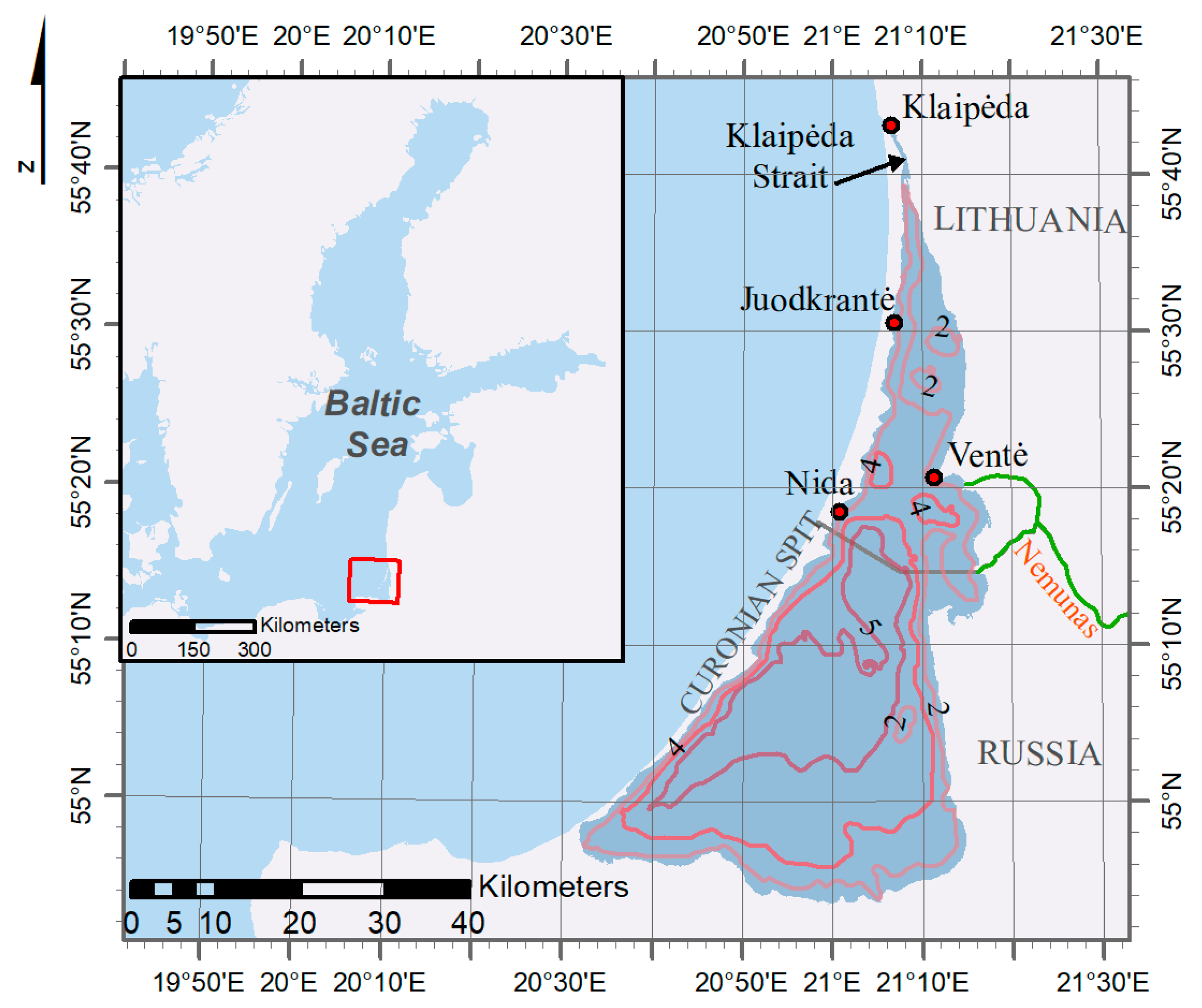
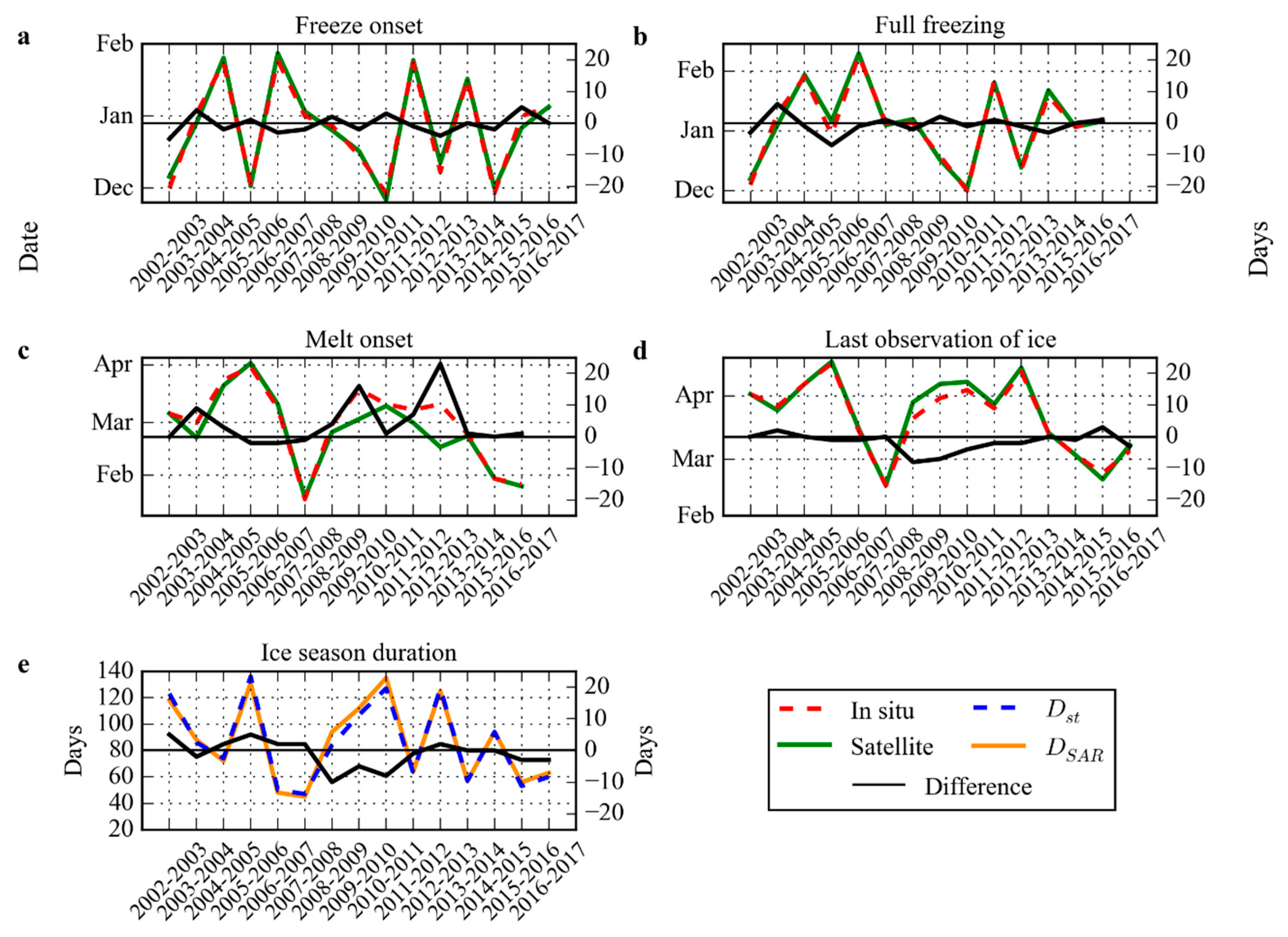
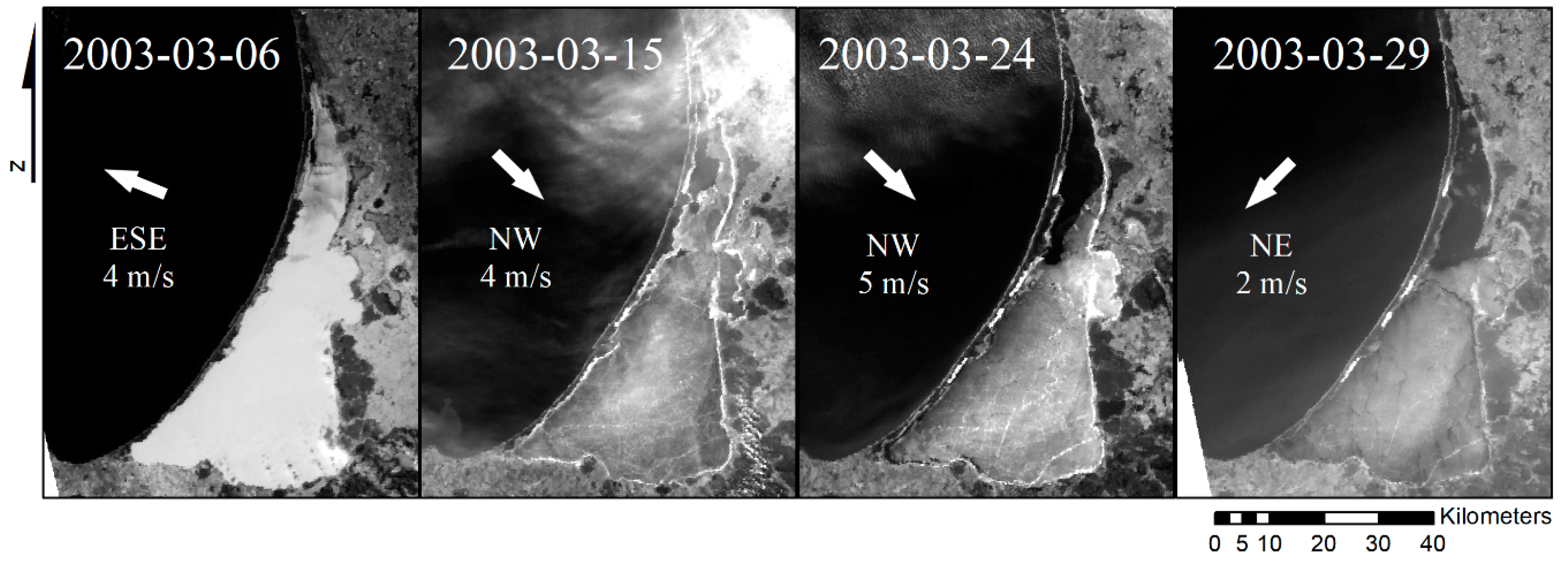
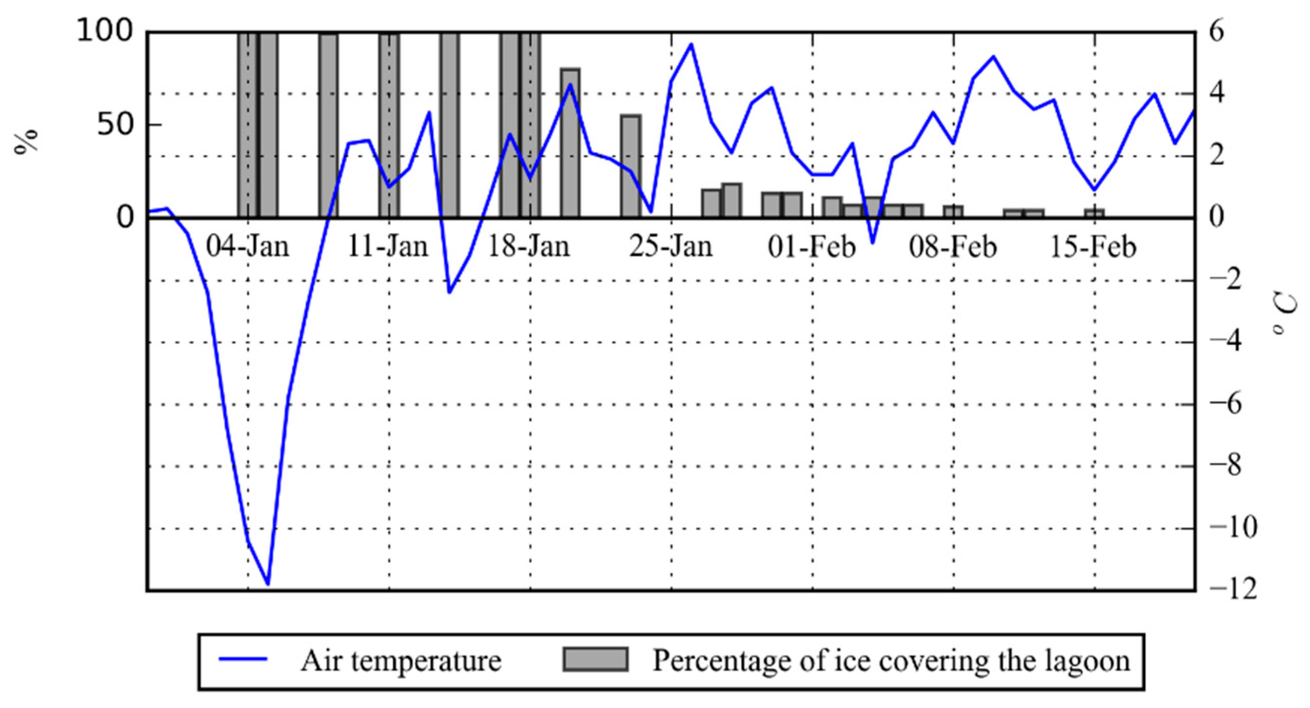
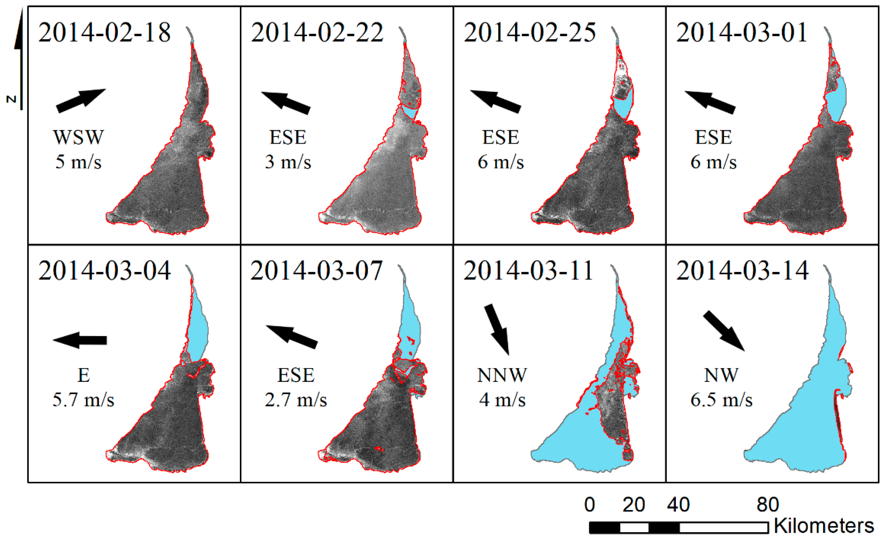
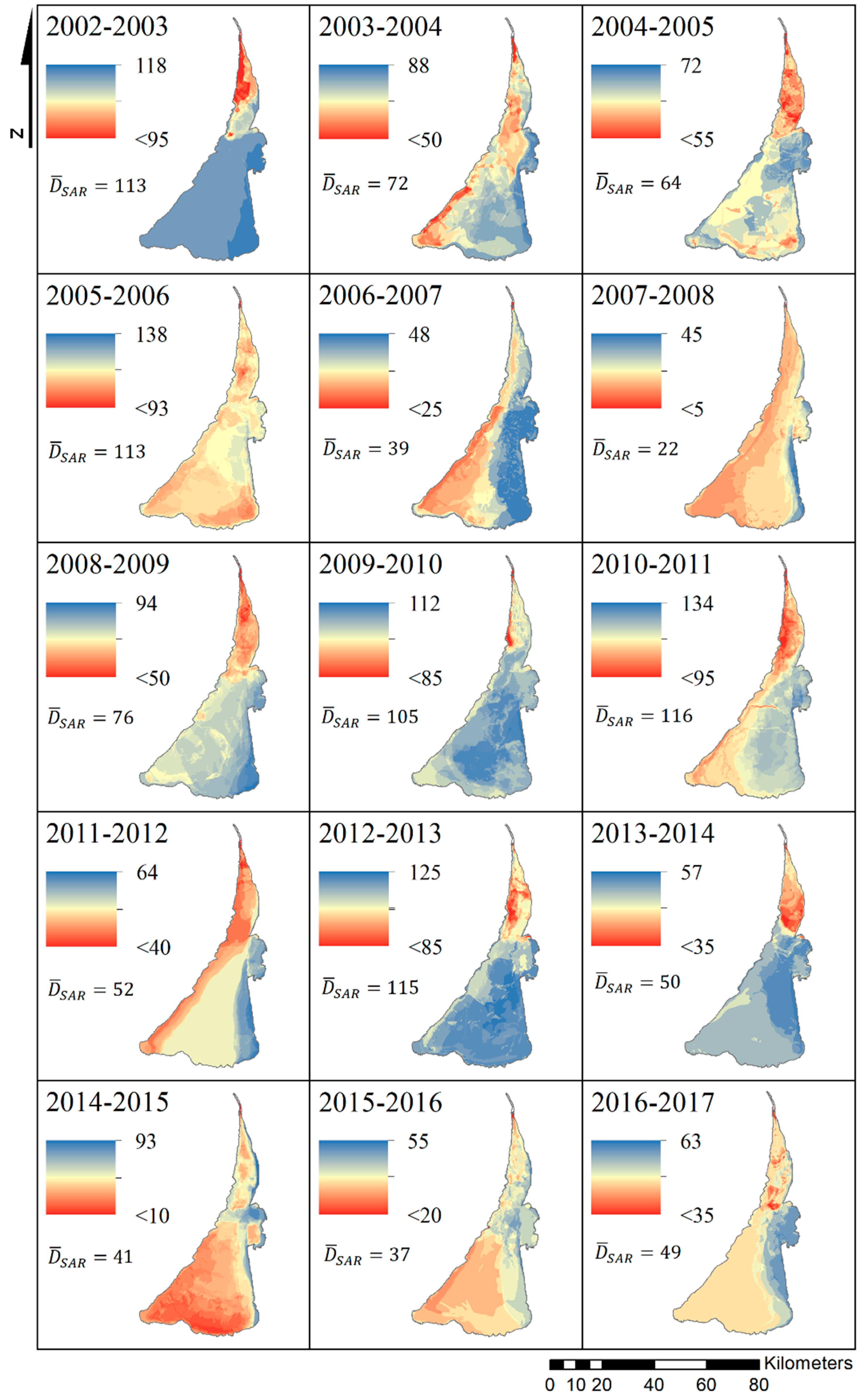
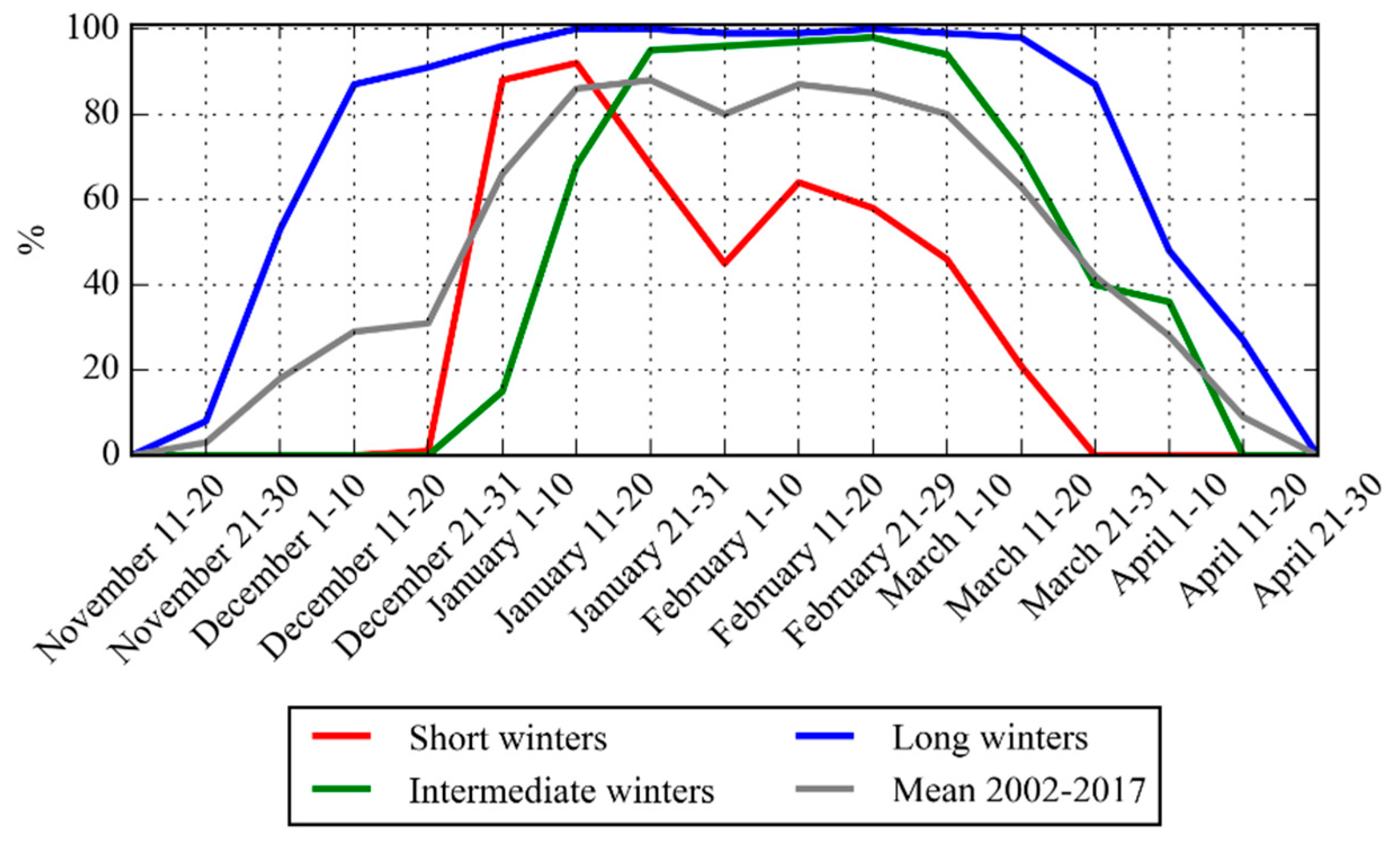
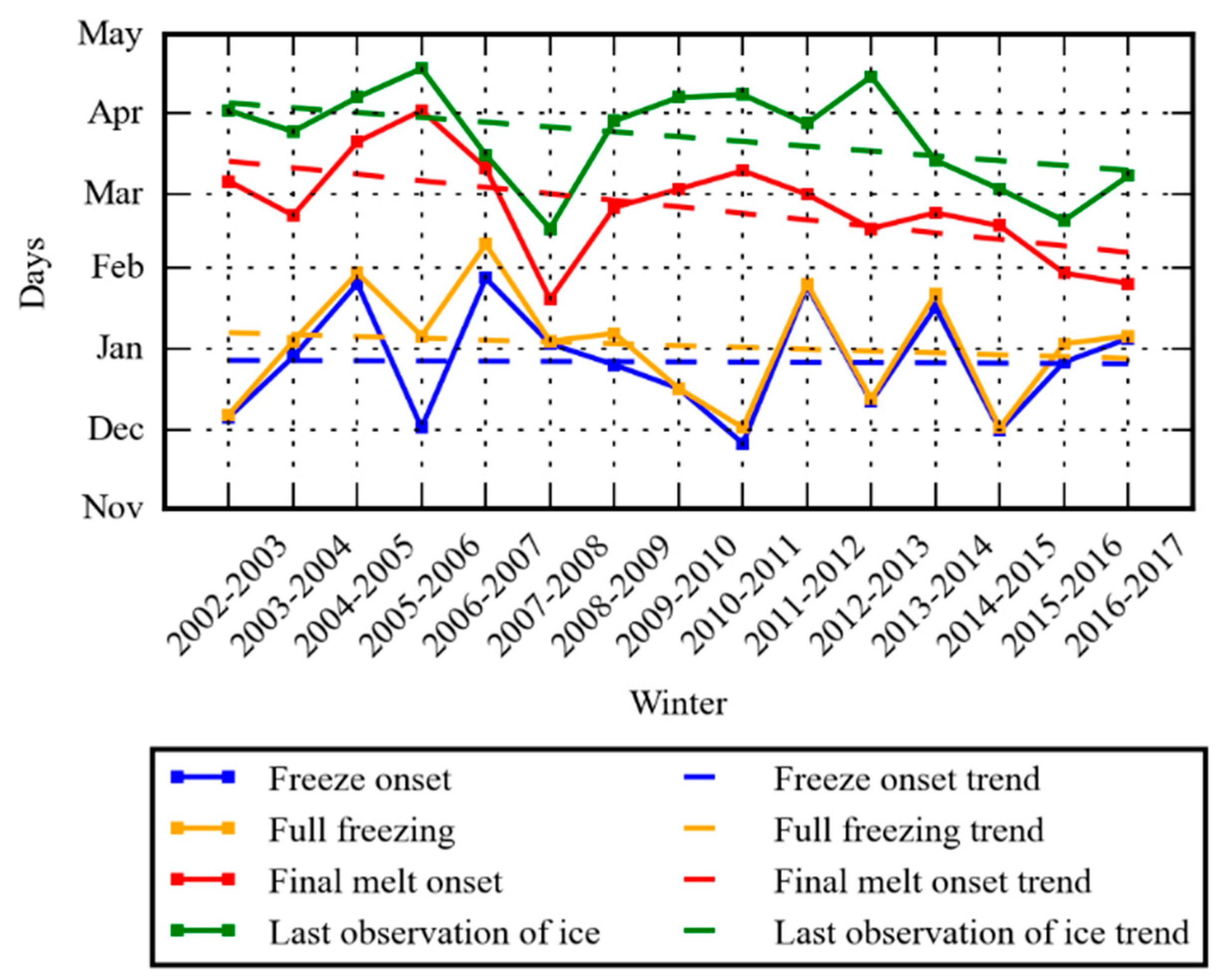
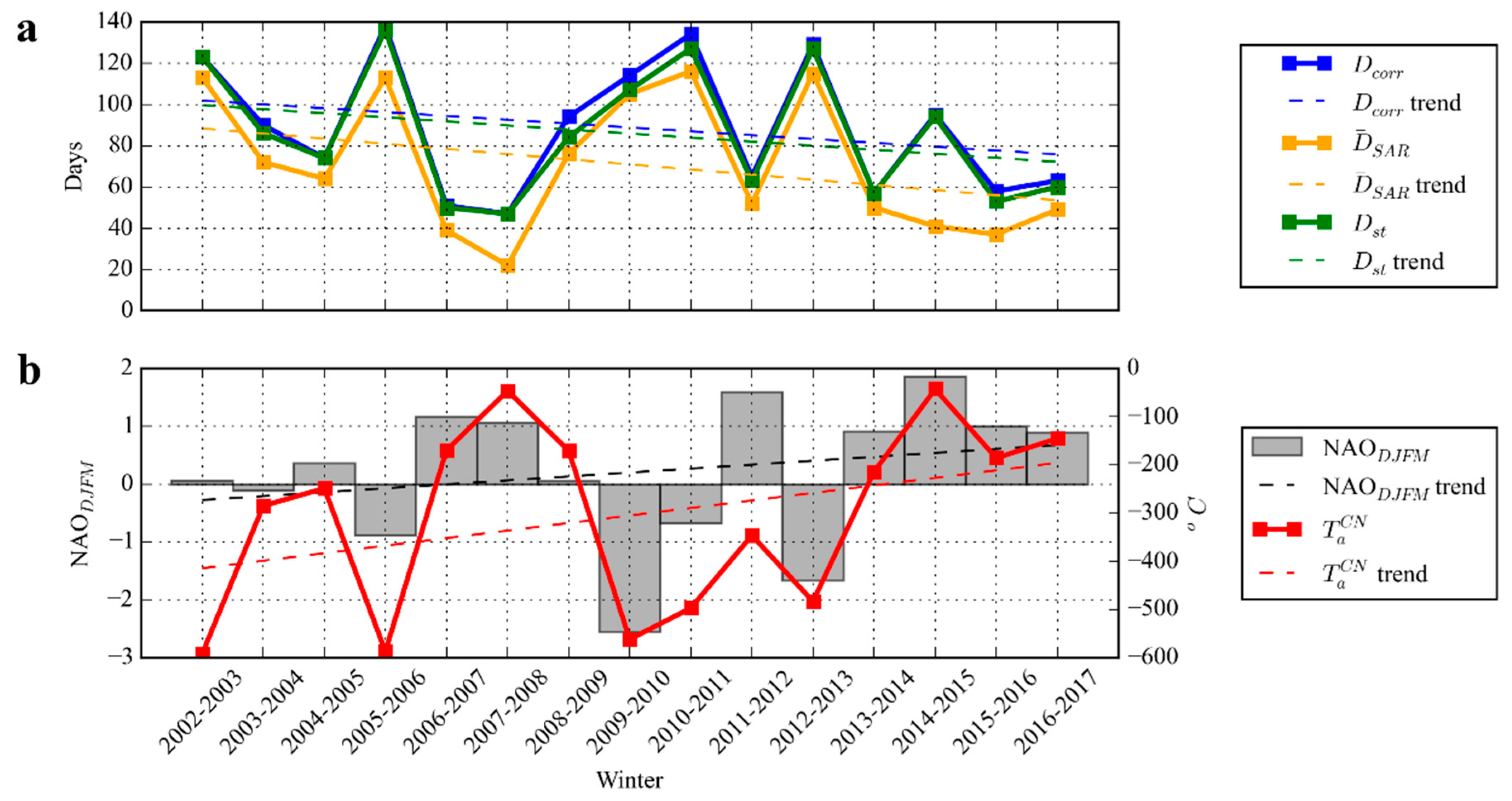
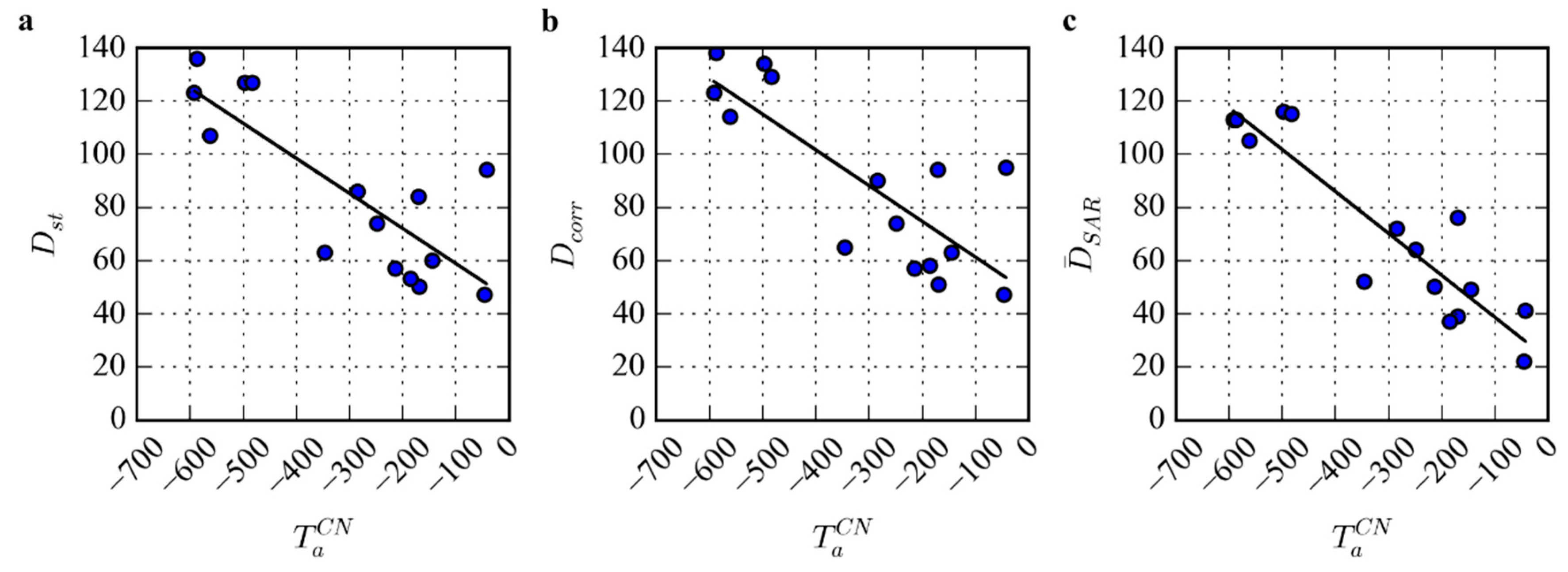
Table 1.
The list and technical characteristics of Earth observation (EO) missions used for the analysis of the ice cover in the Curonian Lagoon. Colors mark specific data sets used during the study period and shown at the bottom of the table, the underlying red lines indicate the available moderate resolution imaging spectroradiometer (MODIS) images.
| Mission | Image Mode | Resolution (m) | Pixel Spacing (m) | Swath Width (km) | Data Coverage |
|---|---|---|---|---|---|
| Envisat Advanced SAR (ASAR) | Wide swath mode (WSM) | 150 × 150 | 75 × 75 | 400 | 2002–2012 April |
| RADARSAT-2 | ScanSAR | 100 × 100 | 50 × 50 | 500 | 2012–2014 April |
| Sentinel-1A | Interferometric Wide swath (IW High) Extra-Wide swath (EW Medium) | 5 × 20, 93 × 87 | 10 × 10, 40 × 40 | 250 400 | November 2014–2017 |
| Sentinel-1B | Interferometric Wide swath (IW High) Extra-Wide swath (EW Medium) | 5 × 20, 93 × 87 | 10 × 10, 40 × 40 | 250 400 | December 2016–2017 |
| MODIS | 250 × 250 | 250 | 2330 | 2002–2007, 2014–2017 |

Table 2.
Summary of the processed satellite data and ice season duration (ISD). is a maximum value of the ISD, —spatial-mean ISD, —maximum value of the ISD observed at the coastal stations, and is a corrected ISD, is a cumulative negative air temperature.
Table 2.
Summary of the processed satellite data and ice season duration (ISD). is a maximum value of the ISD, —spatial-mean ISD, —maximum value of the ISD observed at the coastal stations, and is a corrected ISD, is a cumulative negative air temperature.
| Year | Image Count (+MODIS) | SAR Images per Week (with MODIS) | [days] | [days] | [days] | [days] | [°C] |
|---|---|---|---|---|---|---|---|
| 2002–2003 | 14( + 34) | 0–2(1–5) | 118 | 113 | 123 | 123 | −591.9 |
| 2003–2004 | 12( + 14) | 0–3(0–5) | 88 | 72 | 86 | 90 | −284.7 |
| 2004–2005 | 31( + 15) | 1–3(2–8) | 72 | 64 | 74 | 74 | −248.4 |
| 2005–2006 | 51( + 15) | 1–3(1–7) | 138 | 113 | 136 | 138 | −586.8 |
| 2006–2007 | 20( + 5) | 1–4(2–4) | 48 | 39 | 50 | 51 | −169.4 |
| 2007–2008 | 17( + 5) | 2–3 | 45 | 22 | 47 | 47 | −46.0 |
| 2008–2009 | 50 | 1–3 | 94 | 76 | 84 | 94 | −170.3 |
| 2009–2010 | 53 | 2–3 | 112 | 105 | 107 | 114 | −561.7 |
| 2010–2011 | 55 | 1–3 | 134 | 116 | 127 | 134 | −497.0 |
| 2011–2012 | 46 | 2–4 | 64 | 52 | 63 | 65 | −346.0 |
| 2012–2013 | 56 | 1–3 | 125 | 115 | 127 | 129 | −483.1 |
| 2013–2014 | 32 | 2–3 | 57 | 50 | 57 | 57 | −214.0 |
| 2014–2015 | 27( + 5) | 1–2(1–4) | 93 | 41 | 94 | 95 | −42.5 |
| 2015–2016 | 26( + 5) | 1–2(1–5) | 55 | 37 | 53 | 58 | −185.5 |
| 2016–2017 | 24( + 3) | 2–3(2–4) | 63 | 49 | 60 | 63 | −145.0 |
Table 3.
Statistics in defining the timing of the key stages of the ice formation in the Curonian Lagoon from the satellite observations and coastal records.
Table 3.
Statistics in defining the timing of the key stages of the ice formation in the Curonian Lagoon from the satellite observations and coastal records.
| FO | FF | MO | LOI | ISD | |
|---|---|---|---|---|---|
| Date from in situ | 26 December | 4 January | 1 March | 21 March | 86 |
| Date from satellite data | 27 December | 4 January | 24 February | 23 March | 87 |
| Average difference (days) | −0.46 | −0.62 | 5 | −2.18 | −1.29 |
| Sum of all differences (days) | −6 | −8 | 60 | −24 | −18 |
| Max difference (days) | −5/5 | −7 | 23 | −8 | −10 |
| Satellite success rate (SSR) | 38% | 62% | 75% | 82% | 57% |
| Mean SSR | 63% | ||||
© 2019 by the authors. Licensee MDPI, Basel, Switzerland. This article is an open access article distributed under the terms and conditions of the Creative Commons Attribution (CC BY) license (http://creativecommons.org/licenses/by/4.0/).
Share and Cite
MDPI and ACS Style
Idzelytė, R.; Kozlov, I.E.; Umgiesser, G. Remote Sensing of Ice Phenology and Dynamics of Europe’s Largest Coastal Lagoon (The Curonian Lagoon). Remote Sens. 2019, 11, 2059. https://0-doi-org.brum.beds.ac.uk/10.3390/rs11172059
AMA Style
Idzelytė R, Kozlov IE, Umgiesser G. Remote Sensing of Ice Phenology and Dynamics of Europe’s Largest Coastal Lagoon (The Curonian Lagoon). Remote Sensing. 2019; 11(17):2059. https://0-doi-org.brum.beds.ac.uk/10.3390/rs11172059
Chicago/Turabian StyleIdzelytė, Rasa, Igor E. Kozlov, and Georg Umgiesser. 2019. "Remote Sensing of Ice Phenology and Dynamics of Europe’s Largest Coastal Lagoon (The Curonian Lagoon)" Remote Sensing 11, no. 17: 2059. https://0-doi-org.brum.beds.ac.uk/10.3390/rs11172059
Note that from the first issue of 2016, this journal uses article numbers instead of page numbers. See further details here.