Automated Cloud and Cloud-Shadow Masking for Landsat 8 Using Multitemporal Images in a Variety of Environments


1
Remote Sensing Technology and Data Center, National Institute of Aeronautics and Space of Indonesia (LAPAN), Jakarta 13710, Indonesia
2
Remote Sensing Research Centre, School of Earth and Environmental Scinces (SEES), The University of Queensland, Brisbane 4072, Australia
*
Author to whom correspondence should be addressed.
Remote Sens. 2019, 11(17), 2060; https://0-doi-org.brum.beds.ac.uk/10.3390/rs11172060
Submission received: 15 July 2019
/
Revised: 13 August 2019
/
Accepted: 25 August 2019
/
Published: 2 September 2019
(This article belongs to the Special Issue Remote Sensing: 10th Anniversary)
Abstract
:Landsat 8 images have been widely used for many applications, but cloud and cloud-shadow cover issues remain. In this study, multitemporal cloud masking (MCM), designed to detect cloud and cloud-shadow for Landsat 8 in tropical environments, was improved for application in sub-tropical environments, with the greatest improvement in cloud masking. We added a haze optimized transformation (HOT) test and thermal band in the previous MCM algorithm to improve the algorithm in the detection of haze, thin-cirrus cloud, and thick cloud. We also improved the previous MCM in the detection of cloud-shadow by adding a blue band. In the visual assessment, the algorithm can detect a thick cloud, haze, thin-cirrus cloud, and cloud-shadow accurately. In the statistical assessment, the average user’s accuracy and producer’s accuracy of cloud masking results across the different land cover in the selected area was 98.03% and 98.98%, respectively. On the other hand, the average user’s accuracy and producer’s accuracy of cloud-shadow masking results was 97.97% and 96.66%, respectively. Compared to the Landsat 8 cloud cover assessment (L8 CCA) algorithm, MCM has better accuracies, especially in cloud-shadow masking. Our preliminary tests showed that the new MCM algorithm can detect cloud and cloud-shadow for Landsat 8 in a variety of environments.
1. Introduction
Landsat 8 satellite was launched on 11 February 2013. Landsat 8 images can now be downloaded over the internet at no cost to users from United States Geological Survey (USGS). Recently, the images have been sought and collected by many scientists and researchers, and the total number of images downloaded by users is more than one million from 2014 to 2017 [1]. Landsat 8 images with scene-based Level 1 Precision Terrain (Corrected) (L1TP) data were used in this study. Collection L1TP is radiometrically calibrated and orthorectified using ground control points and digital elevation model (DEM) data and geometric corrections. This level is the highest quality level and the data are suitable for pixel-level time series analysis. Landsat 8 has two main sensors: Operational Land Imager (OLI) and Thermal Infrared Sensor (TIRS) [2].
Landsat 8 images have been widely used for many applications, such as land cover classification [3], agriculture [4,5,6], and disaster monitoring [7,8,9]. Unfortunately, cloud and cloud-shadow cover on the images is an obstacle to further applications. Every year, the average cloud cover over the Earth is about 66% [10]. However, it may differ in each region of the Earth. Clouds and cloud-shadows significantly interfere with optical sensors, such as Landsat. These objects decrease accuracy of remote sensing application results because they obscure the land surface, and the brightening effect of clouds and the darkening effect of cloud-shadows influence the reflectance of each band [11]. Therefore, the development of a robust method for cloud and cloud-shadow is needed to address the issues. The complexity of clouds (e.g., various of cloud types, each type may have a different spectral signature based on cloud properties) and limited Landsat spectral bands makes it difficult to detect clouds [12]. Clouds can be categorized into three types based on the height, i.e., low cloud, middle cloud, and high cloud, and classified visually into 10 classes as presented in Table 1. According to the cloud masking studies, a cloud is frequently classified based on to its thickness, i.e., thin cloud and thick cloud. Thin cloud is more difficult to detect in multispectral satellite images because it is transparent over land [13].
Over recent decades, many cloud and cloud-shadow masking approaches have been developed. We can classify the approaches of cloud and cloud-shadow masking into two categories: Single image-based, and multitemporal image-based. The single image-based approach uses an individual image to detect cloud and cloud-shadow. The existing methods of this approach frequently use a threshold to screen cloud and cloud-shadow. The automatic cloud cover assessment (ACCA) algorithm has been used to detect clouds for Landsat-7 Enhanced Thematic Mapper Plus (ETM+). It helps to schedule the acquisition of Landsat 7 ETM+ of global cloud-free images [15]. The mean and standard deviation of pixel values of the image can be used to obtain the threshold for detecting clouds [16]. To detect haze/cloud in Landsat scenes, a haze-optimized transformation (HOT) was developed [17,18]. Multi-feature combined (MFC) was proposed to detect cloud and cloud-shadow based on spectral, geometric, and texture features [19]. Machine learning, e.g., the spatial procedures for automated removal of cloud and shadow (SPARCS) algorithm based on neural networks have also been used to detect clouds for Landsat [20]. In addition, to handle the big amounts of data, ready-to-use methods based on machine learning techniques to detect cloud, cirrus, snow, shadow, and clear sky pixels in Sentinel-2 MSI images also exist [21]. The function of mask (Fmask) algorithm was developed by integrating a new object-based approach with combined existing approaches to detect cloud, cloud-shadow, and snow at the same time for Landsat and Sentinel-2 images [12,22]. The Fmask is a popular algorithm, which has been used by USGS for L8 CCA (Fmask 3.3 version) to produce Landsat cloud and cloud-shadow masks. The Fmask was improved in detecting cloud and cloud-shadow in mountainous areas for Landsat 4–8 images by integrating digital elevation models (DEMs) [23].
On the other hands, the multitemporal image-based approach uses multiple images from different acquisition dates to detect cloud and cloud-shadow. To highlight pixels that change in the brightness of a derived metric overtime, multitemporal date approaches have the advantage over a single date approach [24]. Moreover, multitemporal image-based approaches have a higher cloud detection accuracy than a single image-based approach [19]. A time-series method for screening cloud and cloud-shadow across Queensland, Australia was developed and compared to Fmask the algorithm. They found that their algorithm had better results in detecting cloud-shadow [25]. To support the monitoring of land cover change, the multi-temporal mask (Tmask) developed for automated masking of cloud, cloud-shadow, and snow for multi-temporal Landsat images [11]. The multi-temporal cloud detection (MTCD) method was developed to detect cloud for FORMOSAT-2, Venμs, Landsat, and Sentinel-2 images [26]. This method works on a pixel-by-pixel basis, which combines a sudden increase of reflectance in the blue wavelength, and a linear correlation of the pixel neighborhoods test taken from couples of images. In response to the limitations of these methods in tropical environments, cloud and cloud-shadow masking using a multi-temporal image approach named multi-temporal cloud masking (MCM) was developed [27]. This approach uses two images: The target image and reference image. The target image has cloud- and cloud-shadow-contaminated pixels and the reference image is a clear image. This approach uses the different reflectance between them to detect cloud and cloud-shadow. The results showed that this approach successfully detected cloud and cloud-shadow with a significantly high accuracy regarding cloud and cloud-shadow masking.
Based on the above overview of current cloud and cloud-shadow masking approaches, automatic identification of cloud and cloud-shadow in a variety of environments remains challenging. In this study, we improved the previous MCM algorithm for application to Landsat 8 images in variety of environments, especially in sub-tropical environments. The improved MCM algorithm was evaluated for Landsat 8 images that have heterogeneous land cover, such as settlement, cropland, open land, forest, mountain, water, and desert, and various cloud types, such as haze, thin cloud, and thick cloud. The improved algorithm was also tested in various environments.
To address this challenge, we focused on the limitation of the previous MCM algorithm. Some limitations of the algorithm were identified after applying it to sub-tropical environments. For instance, increased commission error in desert areas is caused as dust occurs in this area and makes the dark object brighter, thus it is identified as a cloud by the previous MCM algorithm. In the design of the new MCM algorithm, most of the previous MCM algorithm were used. Improvements were made based on the limitation of the previous algorithm. The new MCM algorithm can be used to detect cloud and cloud-shadow in a variety of environments and the accuracies are expected to be significantly high.
2. Material
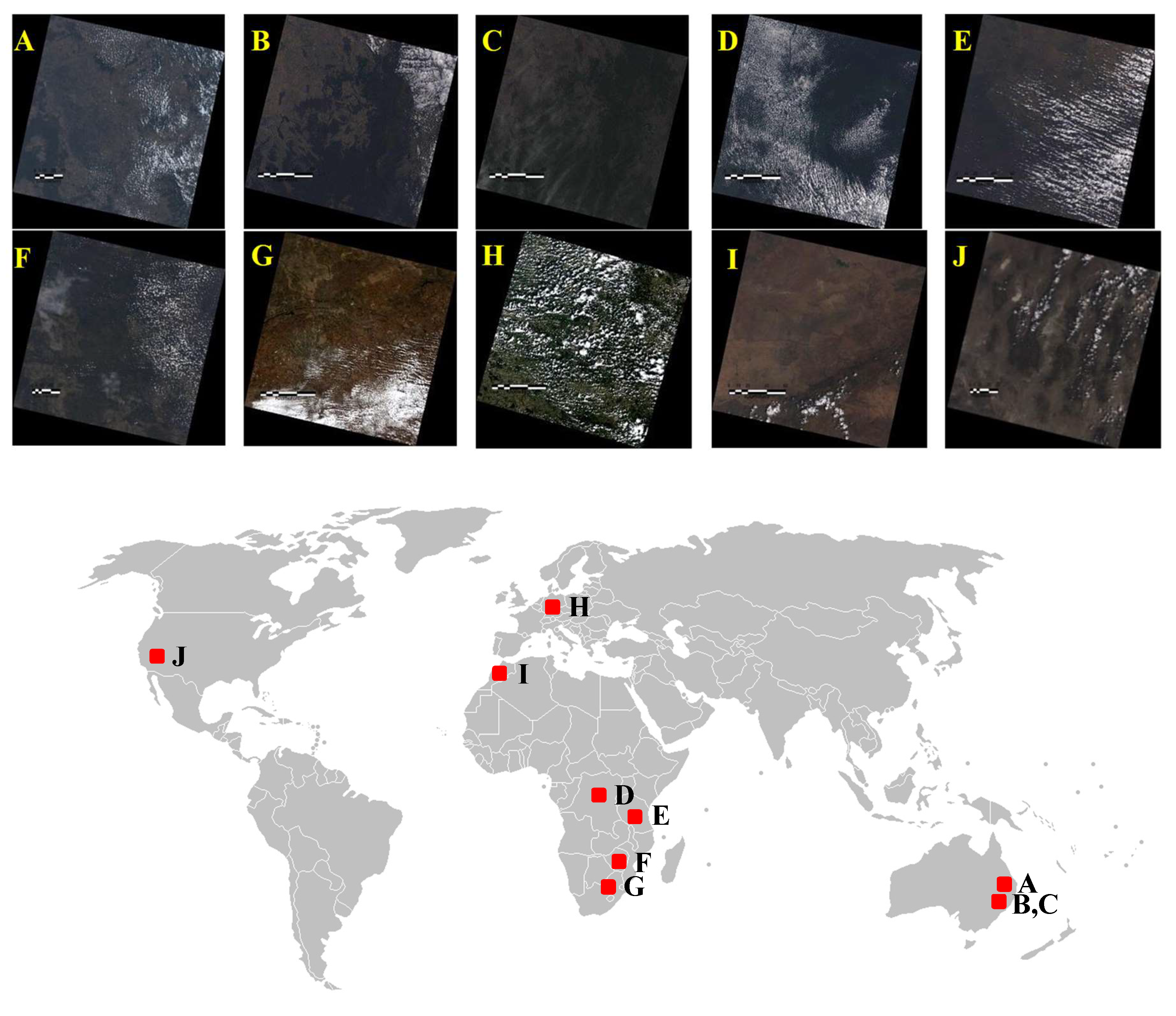
In this study, we used 10 Landsat 8 images, which sample a variety of cloud types, have heterogeneous land cover, and a variety of environments (see Figure 1 and Table 2). Landsat 8 images with scene-based Level-1 Precision Terrain (L1TP) data were used in this study. Collected L1TP are radiometrically calibrated and orthorectified using ground control points and digital elevation model (DEM) data and geometric corrections. This level is the highest quality level and the data are suitable for pixel-level time series analysis.
Landsat 8 has two main sensors: Operational Land Imager (OLI) and Thermal Infrared Sensor (TIRS). We used band 2, 3, 4, 5, 6, and 9 from OLI and band 11 from TIRS to detect cloud and cloud-shadow.
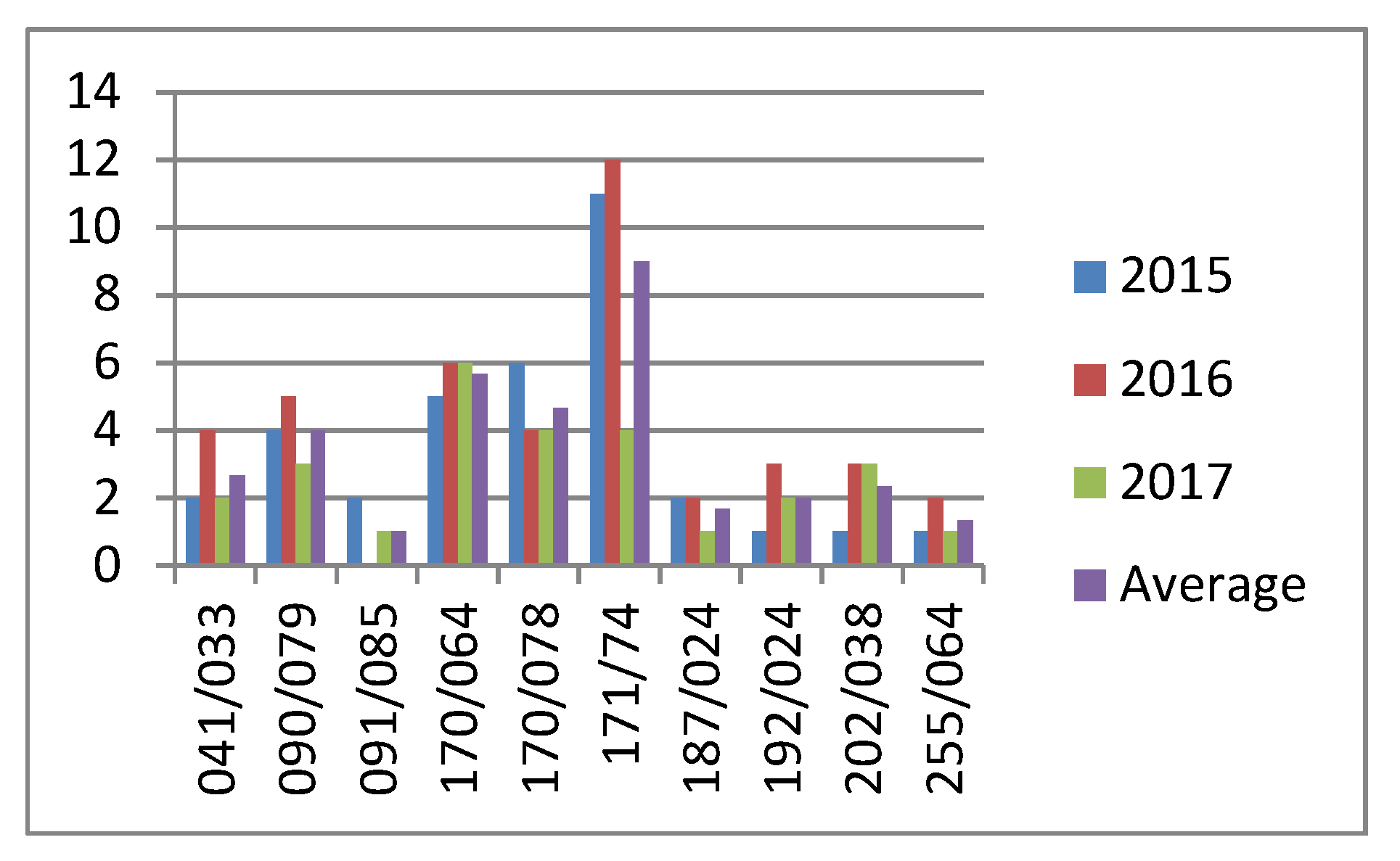
We used two kinds of Landsat-8 images: (1) reference image and (2) target image. The reference image was a clear image and the target image was the image that had cloud and cloud-shadow contaminated pixels. The reference image and target image had an adjacent acquisition date to minimize significant land cover change. In the multitemporal image-based cloud and cloud-shadow masking approach, the main difficulty is to collect a clear image that has the same area as a target image. However, Figure 2 shows that the annual availability of clear images in a variety of environments was sufficient as the average of the availability number of clear images in variety of environments was 3.43 annually. In addition, the highest availability of clear images was 9 on average. It is significantly high, as the total images per year was about 23 images.
3. Methods
3.1. MCM Algorithm Improvements
Multitemporal cloud masking (MCM) was proposed to detect cloud and cloud masking for Landsat 8 in tropical environments using multitemporal images [27]. In this study, we improved this approach to detect cloud and cloud-shadow in an extended range of environments, such as sub-tropical south, tropical, and sub-tropical north. We selected 10 Landsat 8 images to represent the variety of environments. In addition, Table 2 shows the heterogeneous land cover and various cloud types in each scene of Landsat 8. The land cover classes of each scene were determined by using visual interpretation. The basic idea of the MCM algorithm is to utilize the difference between reflectance values of the target image and reference image to detect cloud and cloud-shadow. We chose bands of Landsat 8 that have a big difference in reflectance values between these images. After that, we chose thresholds by using the range of the difference of the reflectance values between these images and conducted some observations to adjust the thresholds to increase the accuracy of the results.
The limitation of the previous MCM is that it was developed only for tropical environments. For instance, in some experiments, the previous MCM generated significant commission errors when detecting cloud in some areas in different environments. The commission error can be caused by land cover change. For example, an object in cropland that is dark on the reference image can change to being brighter on the target image. This usually happens on the object that becomes brighter, such as in cropland area before and after harvest. Therefore, the area is detected as cloud because the difference in the top of atmosphere (TOA) reflectance between them is quite high. The commission error can also be caused by natural phenomena, such as dust in desert areas. It especially occurs in dark objects on desert areas. For instance, an object that is dark on the reference image changes to being brighter due to dust on the target image. The other issue lies in the detection of haze and thin cloud. The previous MCM algorithm failed to detect haze and thin cloud, especially in dark area, such as forest. This increases the omission error.
Issues are also found in the detection of cloud-shadow caused by land cover change and natural phenomena, but the circumstances in cloud-shadow masking are the opposite to the circumstances in the cloud masking described above. Figure 3 shows a flow chart of the new MCM algorithm and details of the improvements of the previous MCM algorithm.
Haze and thin clouds are very difficult to detect due to their transparency, which makes their reflectance values similar to the reflectance values of the Earth’s surface. Haze-optimized transformation (HOT) was introduced for Landsat data in the detection of haze and thin clouds [17]. The basic idea of this algorithm is to utilize the difference between the blue and red wavelengths as their spectral response has high sensitivity. Fmask also uses this algorithm, especially to separate haze and thin cloud. Fmask uses TOA reflectance as inputs in the algorithm.
In this study, we also used the algorithm to improve the ability to detect haze and thin cloud in the previous MCM algorithm. The hot test was used in Fmask, and this approach used 0 for the threshold. In this improved MCM, we slightly changed the threshold to −0.01, as the use of 0 causes omission error in the detection of haze and thin clouds in dark areas, such as forest. Therefore, this change decreased this error:
where Bi(TI) is band i on the target image and Bj(RI) is band j on the reference image.
HOTTest = TI(B1) − 0.5 × TI(B3) − 0.08 > − 0.01
Historically, an issue regarding the detection of cirrus clouds exists as lack of the 1.375-µm wavelength, especially in Landsat ETM+ images. Fortunately, Landsat-8 images have band nine (1.360–1.390 µm), and we used this band to detect cirrus clouds. To make the new MCM more robust in the detection of haze and thin-cirrus clouds, we combined the algorithm with the cirrus band. The use of a small threshold to identify cirrus, such as 0, results in all cirrus being detected but much information of the image is lost. Moreover, the use of a big threshold, such as 0.5, results in the omission error being high. It means that many cirrus clouds still exist in the data. Therefore, we used 0.1 to minimize the omission error. The following algorithm was used for detecting haze and thin-cirrus clouds:
HOTTest > − 0.01 and TI(B9) > 0.01
The presence of a thermal band in Landsat 8 offers a significant advantage for the detection of cloud [12,16,29,30]. We added the thermal band into the previous MCM algorithm to make it more robust, especially in the detection of thick cloud.
Figure 4 shows the range of the brightness temperature of the image in band 10 and band 11. We preferred to use the thermal band from band 11 rather than band 10 because it is narrower and has greater sensitivity to thick cloud. Moreover, we minimized commission error in the detection of cloud by adding band 11 into the cloud masking algorithm. The commission error comes from land cover change between the target image and reference image or natural phenomena, such as dust in a dessert environment, as described above as the issue. In the thermal band, the brightness temperature values of the object that occurred due to land cover change and natural phenomena are almost similar on both the reference image and target image. On the other hand, the brightness temperature value of cloud, especially thick cloud, is usually lower than the temperature of Earth’s surface. Therefore, we used the thermal band to minimize commission error caused by land cover change and natural phenomena. A threshold of 28 (see Figure 4) means that the algorithm produces commission error as the Earth’s surface temperature can reach 28 °C. Therefore, we selected 27 for the threshold of band 11 in detecting thick cloud.
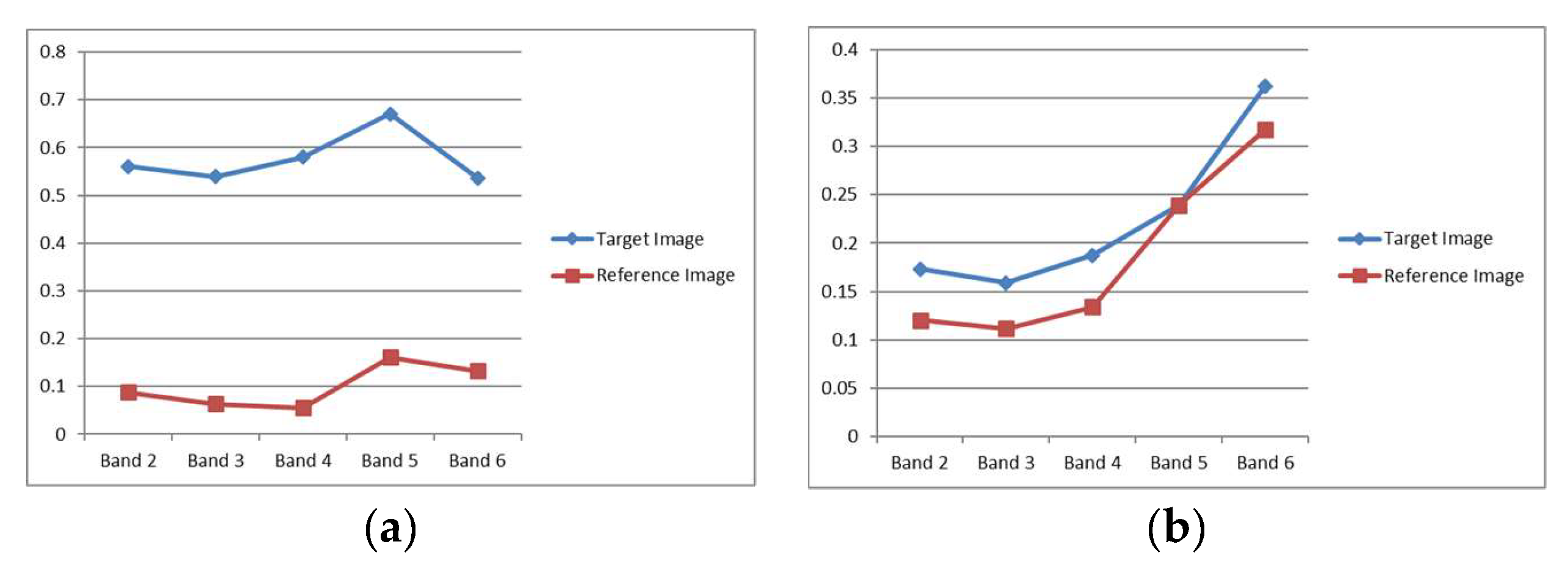
We also improved the previous algorithm for the detection of thick cloud by adding the difference of band two between the target image and reference image. To obtain the threshold, we observed some cloud-contaminated pixels from the center to the edge of the region of cloud. In the center, the difference of the TOA reflectance value between the target image and reflectance image was much bigger than on the edge. Therefore, we chose the difference of the reflectance value on the edge to be a threshold for thick-cloud masking, a value of around 0.04 (see Figure 5). The improved algorithm for thick-cloud masking is shown in Equation (3):
TI(B2) − RI(B2) > 0.04 and TI(B3) − RI(B3) > 0.04 and TI(B4) − RI(B4) > 0.04 and TI(B11) < 27
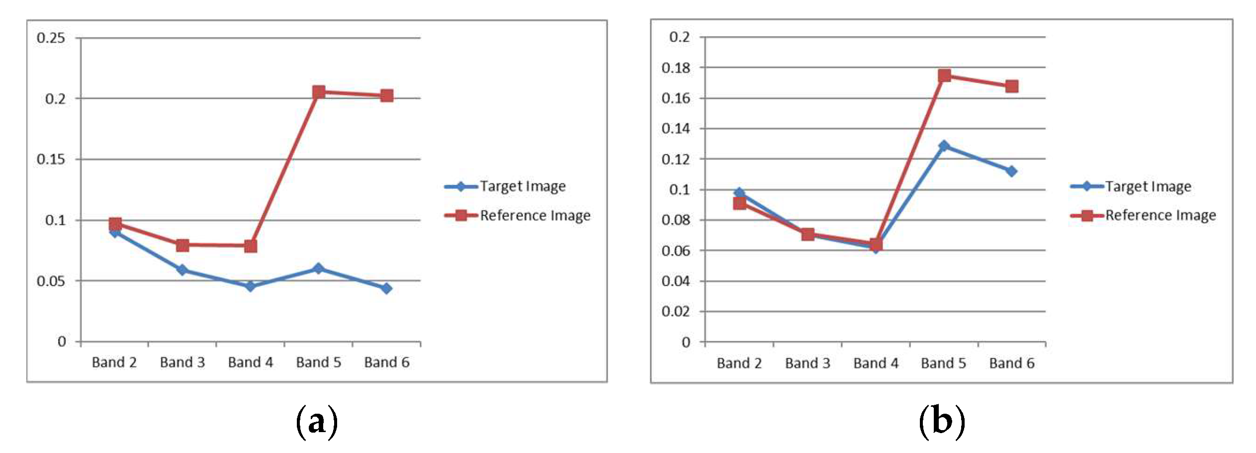
In the previous MCM algorithm, near infrared (NIR) and short-wave infrared (SWIR) were used to detect cloud-shadow for Landsat-8 images. In this study, we improved the previous algorithm by adding the blue band (band two) as cloud-shadows should have band two TOA reflectance that is smaller than 0.11. The aim of this addition was to minimize the commission error of cloud-shadow masking caused by land cover change and natural phenomena as described above. We observed some cloud-shadow-contaminated pixels from the center to the edge of the region of cloud-shadow to obtain the threshold. The difference of the TOA reflectance value between the target image and reflectance image on the center was much bigger than on the edge. Therefore, we decided to choose the difference of the reflectance value on the edge to be a threshold for thick-cloud masking, which was around −0.04 (see Figure 6). The following equation is the improved algorithm for cloud-shadow masking:
TI(B5) − RI(B5) < − 0.04 and TI(B6) − RI(B6) < − 0.04 and TI(B2) < 0.11
In this study, we considered the detection of cloud-shadow in a sea area. By using the improved algorithm above, the omission error was high in the sea area. To address this issue, we developed an algorithm for detecting cloud-shadow in sea areas. This algorithm utilized 30-m DEM SRTM data to separate land and sea. To detect cloud-shadow in the land area, we used the NIR band and SWIR band based on band selection (see Figure 7). In contrary, they are not sensitive in in the detection of cloud-shadow in sea areas because the TOA reflectance values of cloud-shadow in sea areas are very small and the difference between the TOA reflectance of the NIR and SWIR band between the reference image and target image are is very small. To detect cloud-shadow in sea areas, we used visible bands (blue band and green band). Some clouds in the sea area may be detected as cloud-shadow using those bands. Therefore, we also used the NIR band of the target image to minimize this error:
(abs(B2(RI) − B2(TI)) < 0.04 and abs(B3(RI) − B3(TI)) < 0.04 and B5(TI) < 0.012) or (B3(RI) − B3(TI) > 0.04)
3.2. Accuracy Assessment of the New MCM
Visual and statistical assessments were used to evaluate the reliability of the new MCM algorithm for Landsat 8 images. We conducted visual assessment by showing some figures of the results from each environment with different land covers and a variety of cloud types.
To evaluate the quality of the result, in the statistical assessment, we used a confusion matrix [31]. This assessment method can derive the commission error [32] and omission error [24,33]. By using this assessment, we identified the failure percentage of the algorithm in detecting cloud and cloud-shadow.
We selected some samples from each environment with different land covers to evaluate the accuracy of cloud and cloud-shadow masking. In fact, it was difficult to perform an interpretation of the clouds and cloud-shadows, especially at the edge of cloud and cloud-shadow. Therefore, we selected clouds and cloud-shadows that had a distinct edge. The reference data for this assessment was generated using manual digitalization. We manually digitized the cloud and cloud-shadow on the image samples.
3.3. Comparison Between the New MCM and L8 CCA Algorithm
We compared the new MCM and L8 CCA algorithm derived by Landsat Quality Assessment (QA) tools to generate cloud and cloud-shadow masking for Landsat-8 images. The cloud and cloud-shadow masking from this QA band were derived from Fmask 3.3.
4. Results and Discussion
4.1. Visual Assessments of the New MCM Results
We conducted some experiments using Landsat-8 images in a variety of environments, such as sub-tropical south, tropical, and sub-tropical north, to prove the reliability of the new MCM algorithm in the detection of cloud and cloud-shadow. The images also had different land covers and a variety of cloud types. After visually evaluating the results of the new MCM with the color composite RGB 432, it appeared to work well in the detection of cloud (red) and cloud-shadow (blue). We also compared the new MCM algorithm and the previous MCM algorithm to show that the new MCM algorithm improved the ability to detect cloud and cloud-shadow in various environments.
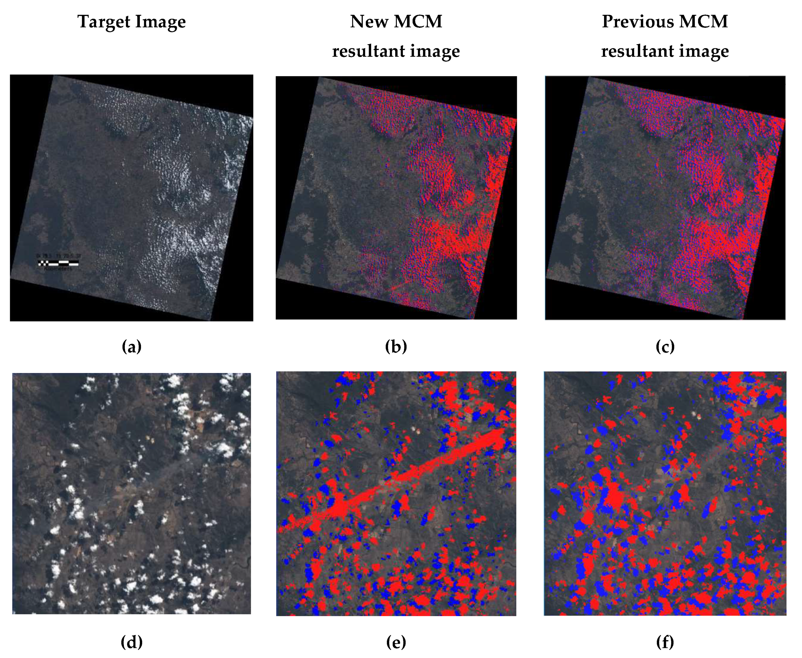
We described the results using figures from each environment with heterogeneous land cover and a variety of cloud types. Figure 8 shows sub-tropical south images with clouds and cloud-shadows over heterogeneous land cover, such as settlement, open land, crop land, forest, water, and mountainous areas. It shows that the new MCM has a strong ability to detect clouds (including thin-cirrus clouds) and cloud-shadows over these land cover types. Figure 8 shows that the algorithm works well in the settlement area. It is difficult to distinguish between cloud and settlement because of their similar brightness levels. This figure shows that the algorithm identified cloud as cloud and settlement as settlement. In addition, it can be seen in Figure 8 that the algorithm can detect cloud-shadow in mountainous areas appropriately. Thin-cirrus cloud can also be detected properly, and it is shown in the middle of Figure 8. In contrary, the previous MCM algorithm failed to identify thin-cirrus cloud. It increased the amount of omission error.
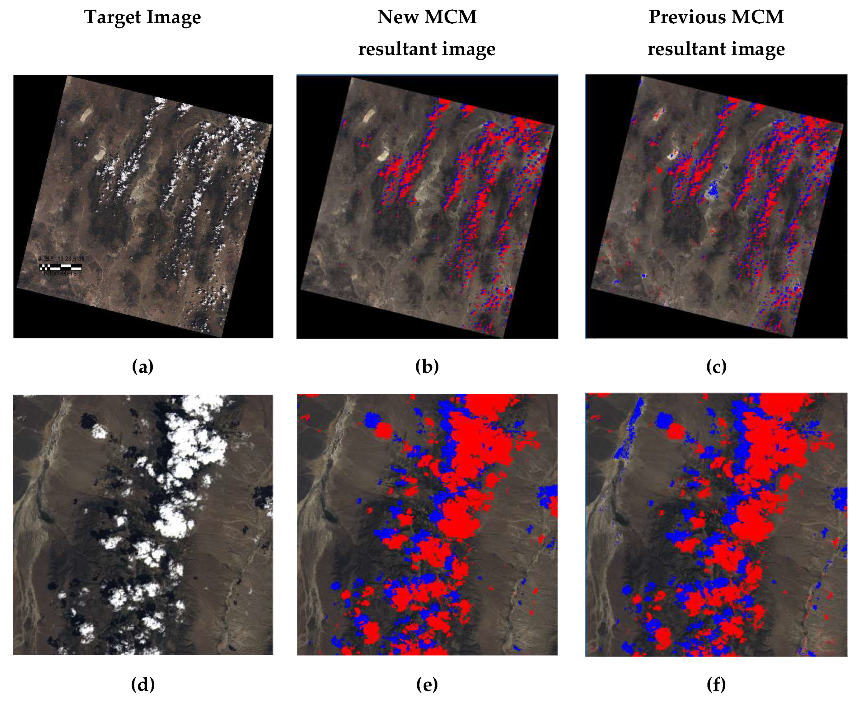
Furthermore, Figure 9 shows the sub-tropical north, which has desert area in most of the image. The new MCM algorithm works well in terms of the detection of cloud in desert areas. It can be seen clearly that the algorithm can also detect very thin cloud in the desert area. There is no issue in identifying cloud-shadow over the desert and mountainous areas. On the other hand, the previous MCM algorithm detected non-cloud-shadow as cloud-shadow. This increased the commission error.
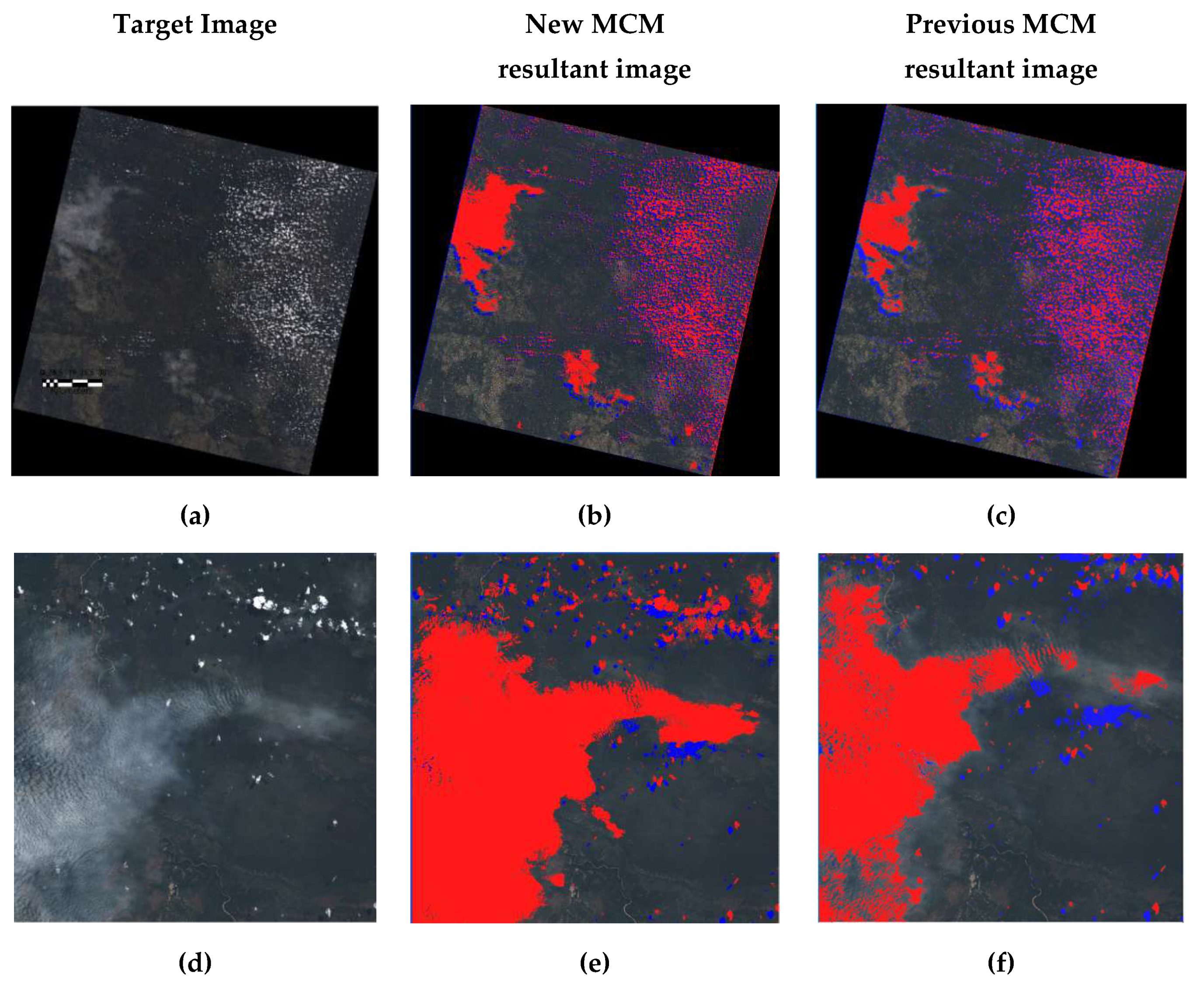
Figure 10 shows the tropical images. This image is quite difficult because it has a large amount of haze and thin clouds over the forest and swamp. It can be seen in Figure 10 that the new MCM algorithm can detect haze and thin cloud accurately. On the other hand, the previous MCM failed to detect a large amount of haze and thin cloud. This increased the omission error.
4.2. Statistical Assessments of the New MCM
In the statistical assessment, we selected some samples of different land cover types, such as settlement, cropland, forest, and desert. The samples were also selected in different environments. The average of the commission error (detected non-cloud as cloud) and omission error (failed to detect cloud) of the new MCM algorithm in detecting cloud was 0.019 and 0.010, respectively, in all scenarios. The highest commission error and omission error of cloud masking was 0.035 and 0.120, respectively, and all the errors were in the forest. It means that the MCM algorithm detected non-cloud as cloud at 0.035 and failed to detect cloud at 0.120. Although the omission error is small enough, it shows that the algorithm has difficulty in distinguishing between cloud and forest, especially in the edge region of cloud. On the other hand, the highest commission error and omission error of cloud-shadow masking was 0.058 and 0.084, respectively. The omission error of 0.084 as in the desert area and it caused the algorithm to fail in identifying cloud-shadow in this area.
Mostly, the area of the commission error and omission error in detecting cloud and cloud-shadow in the edge region of cloud and cloud-shadow caused the algorithm to fail in detecting cloud and cloud-shadow in the region. However, the commission error and omission error in detecting cloud and cloud-shadow were significantly small in all scenarios (see Table 3 and Table 4). It shows that the new MCM algorithm works well in detecting cloud and cloud-shadow.
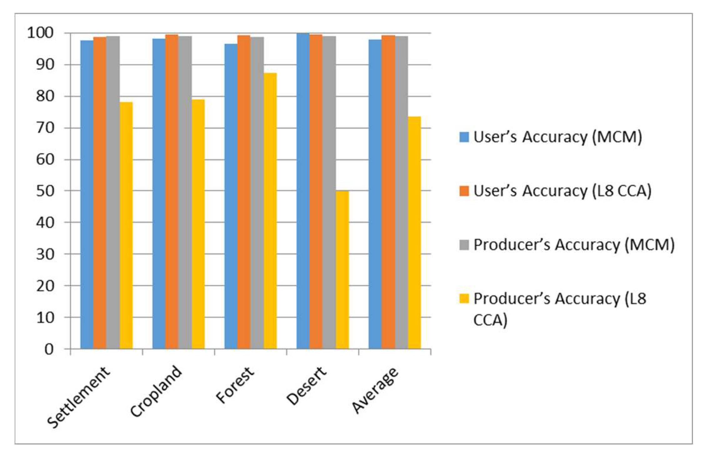
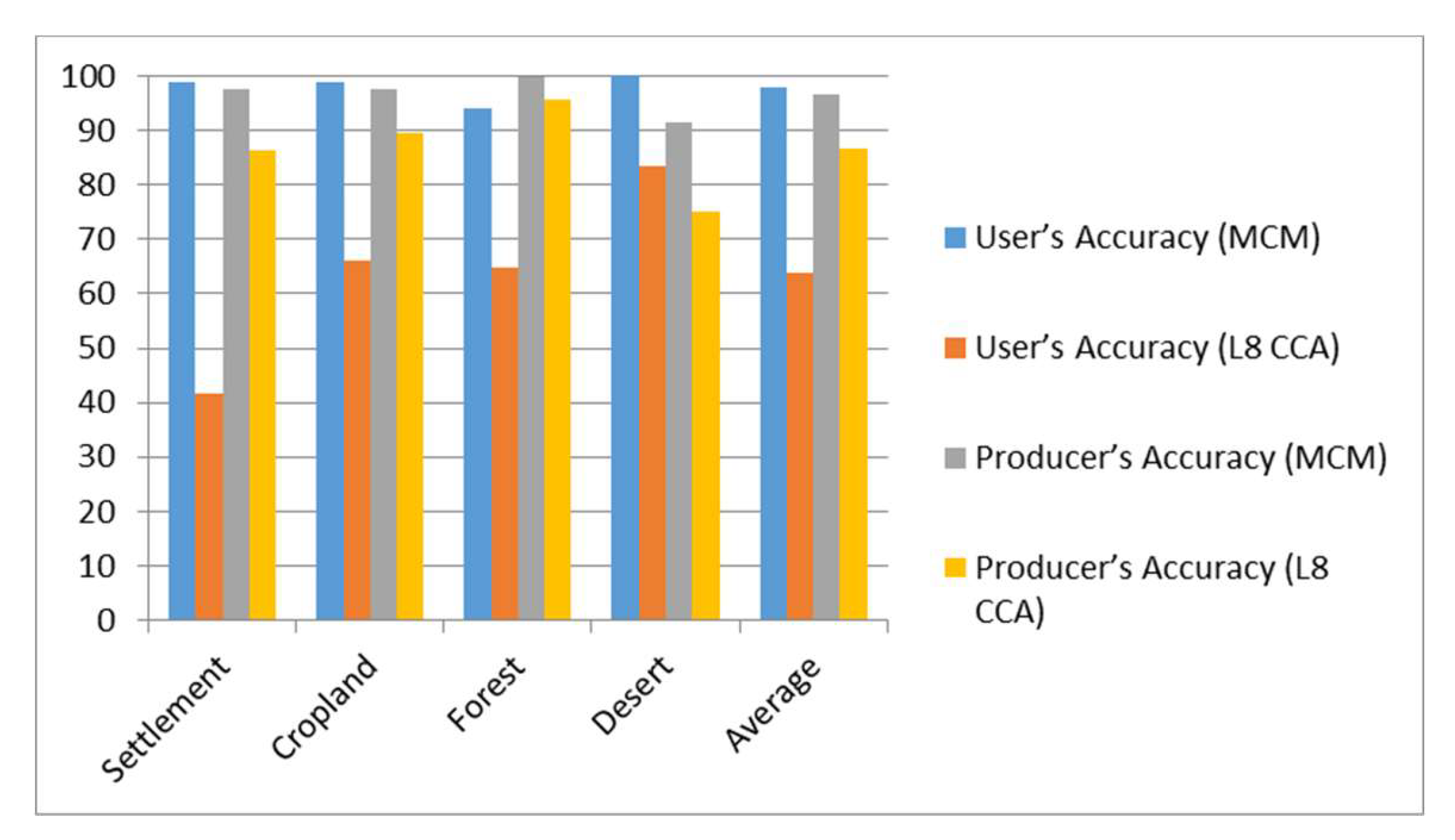
As a result, the average of the user’s accuracy and producer’s accuracy in detecting cloud using the new MCM algorithm was 98.03% and 98.98%, respectively. On the other hand, the algorithm achieved a user’s accuracy and producer’s accuracy for cloud-shadow of 97.97% and 96.66% on average, respectively. Thus, the algorithm works well in terms of detecting cloud and cloud-shadow in all scenarios.
4.3. Comparison Between the New MCM and L8 CCA Algorithm
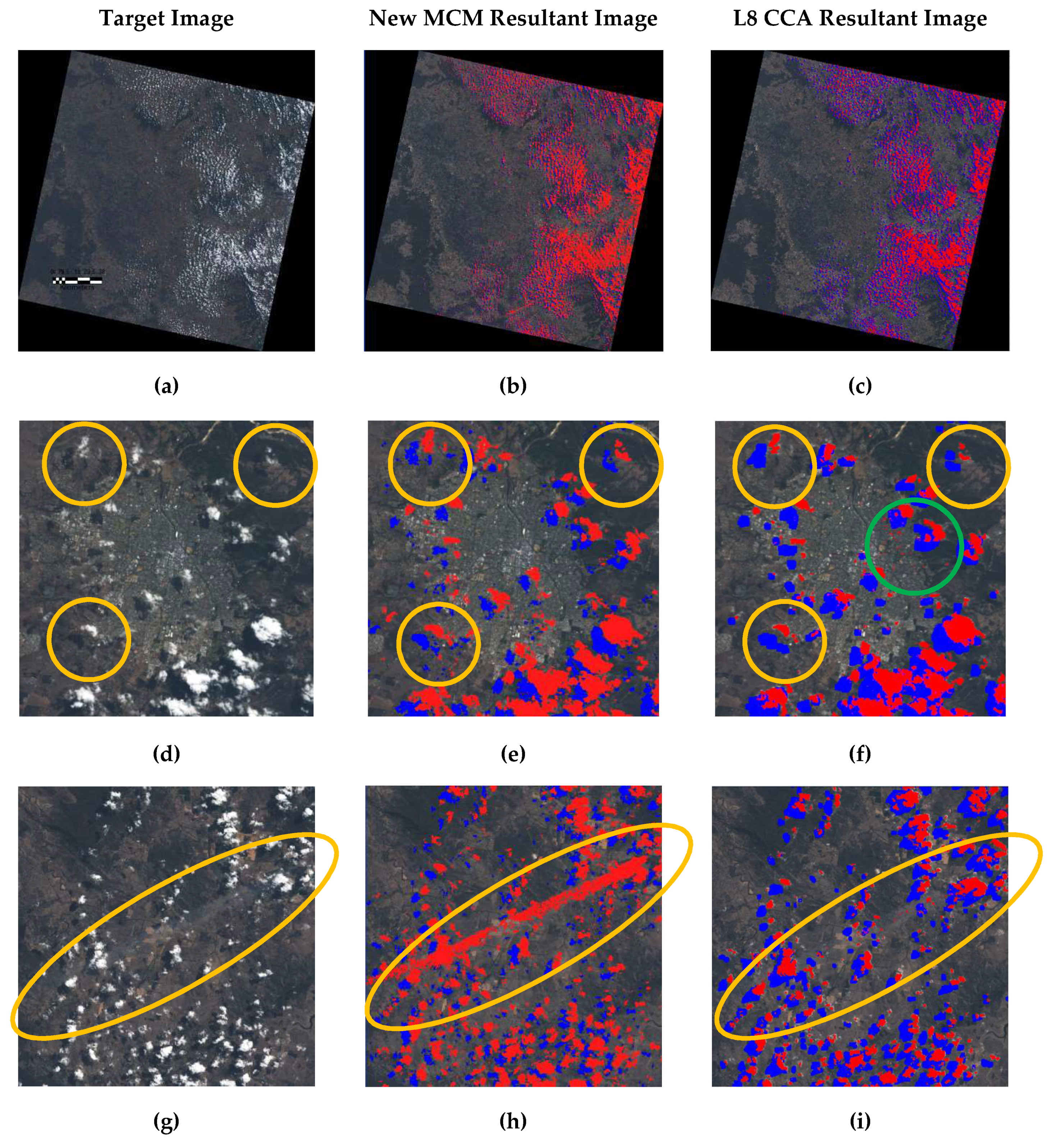
We compared the results of cloud and cloud-shadow masking between the new MCM and L8 CCA. We selected high confidence cloud and cloud-shadow detection of L8 CCA in this process to avoid high commission error in the results. In the visual assessment (see Figure 11 and Figure 12), we can see from the yellow circles on Figure 11 that the new MCM identified cloud and cloud-shadow accurately, but L8 CCA overestimated in identifying cloud-shadow. Moreover, L8 CCA detected non-cloud as a cloud in the settlement area in the green circle. In addition, the yellow ellipse indicates thin-cirrus clouds inside this ellipse and the new MCM can identify the thin-cirrus clouds accurately. On the contrary, the L8 CCA failed to detect most of the thin-cirrus clouds and only detected a few of them. The results showed that the new MCM was better than the L8 ACCA algorithm in cloud detection, especially in the detection of thin-cirrus cloud. In the detection of cloud-shadow, it can be seen clearly in the figures that the L8 CCA algorithm is overly confident. Therefore, the commission error in the detection of cloud-shadow using L8 CCA is higher than the commission error of the new MCM. In addition, the omission error of L8 CCA is also higher than the omission error of the new MCM. Overall, most of the accuracies of the new MCM in the detection of cloud and cloud-shadow are higher than L8 CCA in all scenarios.
Compared to L8 CCA, most of the user’s accuracy and producer’s accuracy of the new MCM had a higher accuracy in detecting cloud, especially in the desert area (see Figure 13). In addition, most of the user’s accuracy and producer’s accuracy of the new MCM was also higher than L8 CCA in the detection of cloud-shadow, especially in the settlement area (see Figure 14).
5. Conclusions and Future Work
This study improved the previous MCM algorithm to detect cloud and cloud-shadow for Landsat 8 in a variety of environments. The new MCM was tested in a variety of environments, such as sub-tropical south, tropical, and sub-tropical north (see Figure 1). Most improvements were found in the detection of clouds. Utilization of the HOT test and thermal band minimized omission error, which caused the failure of the detection of haze and thin-cirrus cloud. They also decreased commission error in the detection of cloud, especially that caused by land cover change and natural phenomena, such as dust in desert areas. By adding band two into the previous algorithm for the detection of cloud masking, the commission error was also decreased, especially in areas that changed to being brighter. From the visual assessment, the resultant images of cloud and cloud-shadow showed that the algorithm detected cloud and cloud-shadow accurately in those environments. Compared to the previous MCM algorithm, the new MCM algorithm was shown to have higher accuracy and it improved the ability to detect cloud and cloud-shadow in various environments (see Figure 8, Figure 9 and Figure 10). The new MCM algorithm was also effective in identifying cloud and cloud-shadow in heterogeneous land and various cloud types. Compared to the L8 CCA, the new MCM can detect cloud and cloud-shadow more accurately during visual inspection, especially in the detection of cirrus cloud and identification of cloud over settlement and desert areas and cloud-shadow over settlement, cropland, forest, and desert areas (see Figure 11 and Figure 12). From the statistical evaluation, the average of the user’s accuracy and the producer’s accuracy of cloud masking using the new-MCM algorithm was 98.03% and 98.98% (see Figure 13). On the other hand, the algorithm’s user’s accuracy and producer’s accuracy in detecting cloud-shadow was 97.97% and 96.66% on average, respectively (see Figure 14). Moreover, compared to L8 CCA, most of the user accuracy’s and producer’s accuracy in screening cloud and cloud-shadow of the new MCM had greater accuracy (see Figure 13 and Figure 14). Therefore, we can conclude that the new MCM can be used to detect cloud and its shadow in a variety of environments with significantly high accuracy. In this study, we tested Landsat 8 images from different parts of the world with a variety of environments, such as settlement, cropland, open land, forest, mountain, water, and desert, to prove the reliability of the algorithm. However, there are still many more places in the world with many kinds of environments that need to be tested. In future research, we would like to test more areas with many kinds of environments to evaluate cloud and cloud-shadow masking ability. The approach also needs automatic optimization of threshold values to handle other images that have a different object spectrum. Therefore, in future research, we will improve the approach to address this issue.
Author Contributions
Conceptualization, D.S.C.; Methodology, D.S.C.; Validation, D.S.C., Formal Analysis, D.S.C.; Investigation, D.S.C.; Resources, D.S.C.; Data Curation, D.S.C.; Writing – Original Draft Preparation, D.S.C.; Writing – Review & Editing, D.S.C., S.P., and P.S.; Visualization, D.S.C.; Supervision, S.P., and P.S.
Funding
This publication was supported by Indonesian Ministry of Research, Technology, and Higher Education, grant number 14/INS-1/PPK/E4/2019 (INSINAS 2019).
Acknowledgments
The authors would like to thank and appreciate the anonymous reviewers. The authors would like to thank the U.S. Geological Survey (USGS) for providing Landsat 8 images as well. The authors also would like to thank Remote Sensing Technology and Data Center, National Institute of Aeronautics and Space (LAPAN) and Remote Sensing Research Centre, The University of Queensland for their support.
Conflicts of Interest
The authors declare no conflict of interest.
Abbreviations
The following abbreviations are used in this manuscript:
| MCM | Multitemporal Cloud Masking | DEM | Digital Elevation Model |
| L8 CCA | Landsat 8 Cloud Cover Assessment | OLI | Operational Land Imager |
| USGS | The U.S. Geological Survey | TIRS | Thermal Infrared Sensor |
| HOT | Haze Optimized Transformation | MTCD | Multitemporal Cloud Detection |
| Fmask | Function of Mask | L1TP | Level-1 Precision Terrain |
| Tmask | multiTemporal mask |
References
- USGS. Landsat Project Statistics. Available online: https://landsat.usgs.gov/landsat-project-statistics (accessed on 7 July 2018).
- USGS. Landsat 8 Data Users Handbook. Available online: https://landsat.usgs.gov/landsat-8-data-users-handbook (accessed on 7 July 2018).
- Jia, K.; Wei, X.; Gu, X.; Yao, Y. Land cover classification using Landsat 8 Operational Land Imager data in Beijing, China. Geocarto Int. 2014, 29, 1–15. [Google Scholar] [CrossRef]
- Chejarla, V.R.; Mandla, V.R.; Palanisamy, G.; Choudhary, M. Estimation of damage to agriculture biomass due to Hudhud cyclone and carbon stock assessment in cyclone affected areas using Landsat-8. Geocarto Int. 2017, 32, 589–602. [Google Scholar] [CrossRef]
- Ozelkan, E.; Chen, G.; Ustundag, B.B. Multiscale object-based drought monitoring and comparison in rainfed and irrigated agriculture from Landsat 8 OLI imagery. Int. J. Appl. Earth Obs. Geoinf. 2016, 44, 159–170. [Google Scholar] [CrossRef]
- Torbick, N.; Chowdhury, D.; Salas, W.; Qi, J. Monitoring rice agriculture across myanmar using time series Sentinel-1 assisted by Landsat-8 and PALSAR-2. Remote Sens. 2017, 9, 119. [Google Scholar] [CrossRef]
- Chignell, S.; Anderson, R.S.; Evangelista, P.H.; Laituri, M.J.; Merritt, D.M. Multi-Temporal Independent Component Analysis and Landsat 8 for Delineating Maximum Extent of the 2013 Colorado Front Range Flood. Remote Sens. 2015, 7, 9822–9843. [Google Scholar] [CrossRef] [Green Version]
- Dao, P.; Liou, Y.A. Object-Based Flood Mapping and Affected Rice Field Estimation with Landsat 8 OLI and MODIS Data. Remote Sens. 2015, 7, 5077–5097. [Google Scholar] [CrossRef] [Green Version]
- Olthof, I.; Tolszczuk-Leclerc, S. Comparing Landsat and RADARSAT for Current and Historical Dynamic Flood Mapping. Remote Sens. 2018, 10, 780. [Google Scholar] [CrossRef]
- Wang, B.; Ono, A.; Muramatsu, K.; Fujiwara, N. Automated detection and removal of cloud and their shadow from Landsat TM images. IEICE Trans. Inf. Syst. 1999, E82-D, 453–460. [Google Scholar]
- Zhu, Z.; Woodcock, C.E. Automated cloud, cloud shadow and snow detection in multitemporal Landsat data: An algorithm designed specifically for monitoring land cover change. Remote Sens. Environ. 2014, 152, 217–234. [Google Scholar] [CrossRef]
- Zhu, Z.; Woodcock, C.E. Object-based cloud and cloud shadow detection in Landsat imagery. Remote Sens. Environ. 2012, 118, 83–94. [Google Scholar] [CrossRef]
- Richter, R.; Wang, X.; Bachmann, M.; Schlapfer, D. Correction of cirrus effects in Sentinel-2 type of imagery. Int. J. Remote Sens. 2011, 32, 2931–2941. [Google Scholar] [CrossRef]
- Houze, R.A. Chapter 1—Types of Clouds in Earth’s Atmosphere. In International Geophysics; Houze, R.A., Ed.; Academic Press: Cambridge, MA, USA, 2014; p. 5. [Google Scholar]
- Irish, R.R.; Barker, J.L.; Goward, S.N.; Arvidson, T. Characterization of the Landsat-7 ETM+ Automated Cloud-Cover Assessment (ACCA) algorithm. Photogramm. Eng. Remote Sens. 2006, 72, 1179–1188. [Google Scholar] [CrossRef]
- Huang, C.; Thomas, N.; Goward, S.N.; Masek, J. Automated masking of cloud and cloud shadow for forest change analysis using Landsat images. Int. J. Remote Sens. 2010, 31, 5449–5464. [Google Scholar] [CrossRef]
- Zhang, Y.; Guindon, B.; Cihlar, J. An image transform to characterize and compensate for spatial variations in thin cloud contamination of Landsat images. Remote Sens. Environ. 2002, 82, 173–187. [Google Scholar] [CrossRef]
- Zhang, Y.; Guindon, B.; Li, X. A Robust Approach for Object-Based Detection and Radiometric Characterization of Cloud Shadow Using Haze Optimized Transformation. IEEE Trans. Geosci. Remote Sens. 2014, 52, 5540–5547. [Google Scholar] [CrossRef]
- Li, Z.; Shen, H.; Li, H.; Xia, G.; Gamba, P.; Zhang, L. Multi-feature combined cloud and cloud shadow detection in GaoFen-1 wide field of view imagery. Remote Sens. Environ. 2017, 191, 342–358. [Google Scholar] [CrossRef] [Green Version]
- Hughes, M.J.; Daniel, J.H. Automated Detection of Cloud and Cloud Shadow in Single-Date Landsat Imagery Using Neural Networks and Spatial Post-Processing. Remote Sens. 2014, 6, 4907–4926. [Google Scholar] [CrossRef] [Green Version]
- André, H.; Segl, K.; Guanter, L.; Brell, M.; Enesco, M. Ready-to-Use Methods for the Detection of Clouds, Cirrus, Snow, Shadow, Water and Clear Sky Pixels in Sentinel-2 MSI Images. Remote Sens. 2016, 8, 666. [Google Scholar] [Green Version]
- Zhu, Z.; Wang, S.; Woodcock, C.E. Improvement and expansion of the Fmask algorithm: cloud, cloud shadow, and snow detection for Landsats 4–7, 8, and Sentinel 2 images. Remote Sens. Environ. 2015, 159, 269–277. [Google Scholar] [CrossRef]
- Qiu, S.; He, B.; Zhu, Z.; Liao, Z.; Quan, X. Improving Fmask cloud and cloud shadow detection in mountainous area for Landsats 4-8 images. Remote Sens. Environ. 2017, 199, 107–119. [Google Scholar] [CrossRef]
- Kennedy, R.E.; Cohen, W.B.; Schroeder, T.A. Trajectory-based change detection for automated characterization of forest disturbance dynamics. Remote Sens. Environ. 2007, 110, 370–386. [Google Scholar] [CrossRef]
- Goodwin, N.R.; Collet, L.J.; Denham, R.J.; Flood, N.; Tindall, D. Cloud and cloud shadow screening across Queensland, Australia: An automated method for Landsat TM/ETM+ time series. Remote Sens. Environ. 2013, 134, 50. [Google Scholar] [CrossRef]
- Hagolle, O.; Huc, M.; Pascual, V.; Dedieu, G. A multi-temporal method for cloud detection, applied to FORMOSAT-2, VENµS, LANDSAT and SENTINEL-2 images. Remote Sens. Environ. 2010, 114, 1747–1755. [Google Scholar] [CrossRef]
- Candra, D.S.; Phinn, S.; Scarth, P. Cloud and cloud shadow masking using multi-temporal cloud masking algorithm in tropical environmental. ISPRS Int. Arch. Photogramm. Remote Sens. Spat. Inf. Sci. 2016, XLI-B2. [Google Scholar] [CrossRef]
- Wikimedia. Maps of the World. Available online: https://commons.wikimedia.org/wiki/Maps_of_the_world#/media/File:BlankMap-World-v2.png (accessed on 19 March 2019).
- Huang, C.; Goward, S.N.; Masek, J.G.; Thomas, N.; Zhu, Z.; Vogelmann, J.E. An automated approach for reconstructing recent forest disturbance history using dense Landsat time series stacks. Remote Sens. Environ. 2010, 114, 183–198. [Google Scholar] [CrossRef]
- Masek, J.G.; Vermote, E.F.; Saleous, N.E.; Wolfe, R.; Hall, F.G.; Huemmerich, K.F.; Gao, F.; Kutler, J.; Kim, T.K. A Landsat surface reflectance dataset for North America, 1990-2000. IEEE Geosci. Remote Sens. Lett. 2006, 3, 68–72. [Google Scholar] [CrossRef]
- Congalton, R.G. A review of assessing the accuracy of classifications of remotely sensed data. Remote Sens. Environ. 1991, 37, 35–46. [Google Scholar] [CrossRef]
- Immitzer, M.; Vuolo, F.; Atzberger, C. First Experience with Sentinel-2 Data for Crop and Tree Species Classifications in Central Europe. Remote Sens. 2016, 8, 166. [Google Scholar] [CrossRef]
- Congalton, R.G.; Green, K. Assessing the Accuracy of Remotely Sensed Data: Principles and Practices; Lewis Publishers: Boca Raton, FL, USA, 1999. [Google Scholar]
Figure 1.
Landsat 8 images were selected in a global area with a variety of cloud types and different environments in sub-tropical south, tropical, and sub-tropical north. The scenes of Landsat 8 images are shown by the red color. (adapted from [28]).
Figure 1.
Landsat 8 images were selected in a global area with a variety of cloud types and different environments in sub-tropical south, tropical, and sub-tropical north. The scenes of Landsat 8 images are shown by the red color. (adapted from [28]).

Figure 2.
The annual availability of clear images of Landsat-8 in a variety of environments (sub-tropical south, tropical, and sub-tropical north). X-axis is path/row and Y-axis is the total number of clear images.
Figure 2.
The annual availability of clear images of Landsat-8 in a variety of environments (sub-tropical south, tropical, and sub-tropical north). X-axis is path/row and Y-axis is the total number of clear images.

Figure 3.
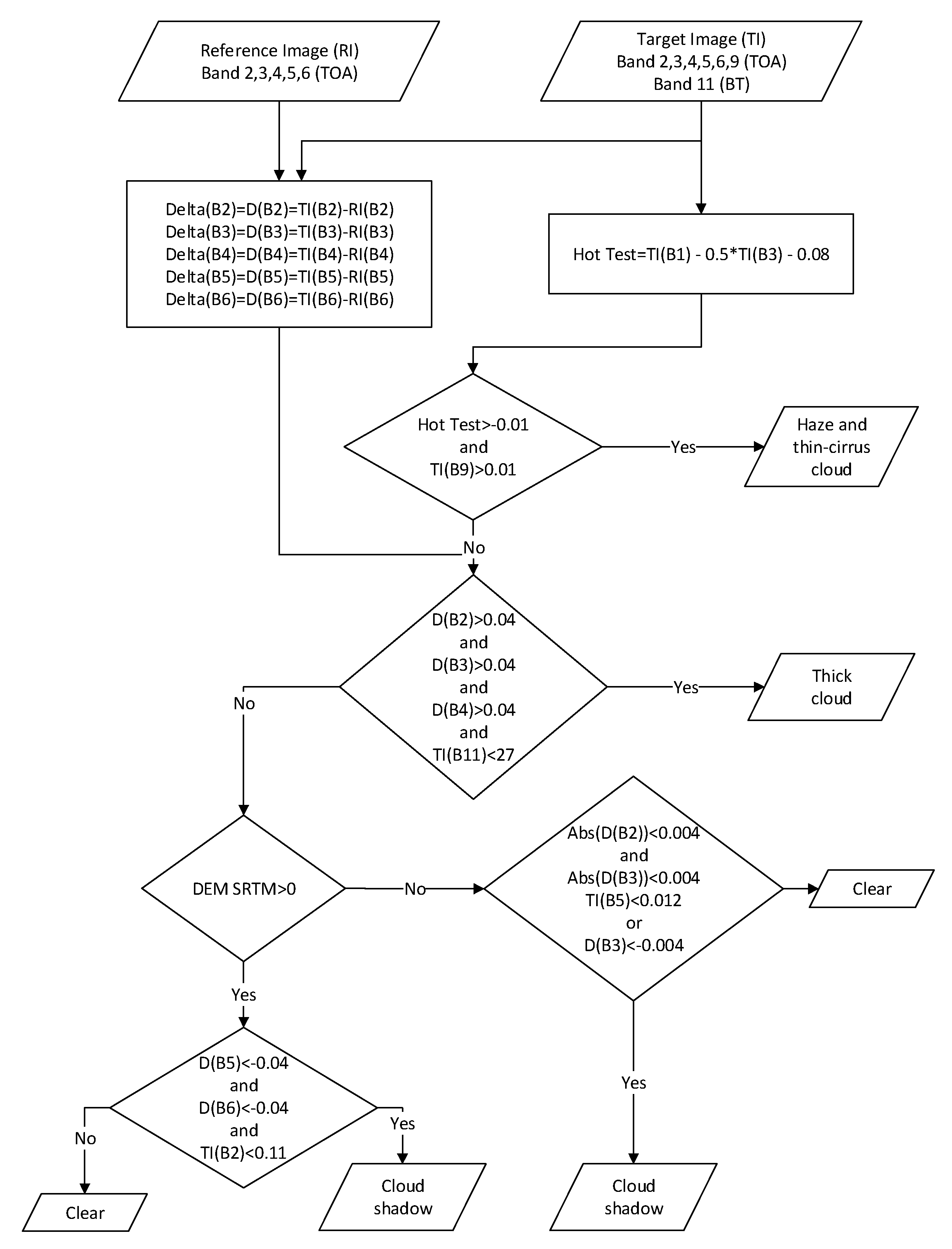
The flowchart of the new Multitemporal Cloud Masking (MCM) algorithm for Landsat 8. TI(Bi) is band i in the target image and RI(Bj) is band j in the reference image. Abs(D(X)) is the absolute value of D(X). B2, B3, B4, B5, B6, B9, and B11 represent the blue, green, red, near infrared, shortwave infrared, cirrus, and thermal bands in Landsat 8, respectively.
Figure 3.
The flowchart of the new Multitemporal Cloud Masking (MCM) algorithm for Landsat 8. TI(Bi) is band i in the target image and RI(Bj) is band j in the reference image. Abs(D(X)) is the absolute value of D(X). B2, B3, B4, B5, B6, B9, and B11 represent the blue, green, red, near infrared, shortwave infrared, cirrus, and thermal bands in Landsat 8, respectively.

Figure 4.
The cloud image sample on path/row 090/079. (a) The sample of thick cloud, (b) The brightness temperature (BT) of the image (a) in band 10 ranges from 16 to 30, and (c) Band 11 ranges from 16 to 28 (bottom).
Figure 4.
The cloud image sample on path/row 090/079. (a) The sample of thick cloud, (b) The brightness temperature (BT) of the image (a) in band 10 ranges from 16 to 30, and (c) Band 11 ranges from 16 to 28 (bottom).

Figure 5.
Band selection and obtaining the threshold for thick-cloud masking from the Top of Atmospheric (TOA) reflectance of the selected pixel on: (a) the center of the cloud region and (b) the edge of the cloud region.
Figure 5.
Band selection and obtaining the threshold for thick-cloud masking from the Top of Atmospheric (TOA) reflectance of the selected pixel on: (a) the center of the cloud region and (b) the edge of the cloud region.

Figure 6.
Band selection and obtaining the threshold for cloud-shadow masking from the TOA reflectance of the selected pixel on: (a) the center of the cloud region and (b) the edge of the cloud region.
Figure 6.
Band selection and obtaining the threshold for cloud-shadow masking from the TOA reflectance of the selected pixel on: (a) the center of the cloud region and (b) the edge of the cloud region.

Figure 7.
Band selection and obtaining the threshold for cloud-shadow masking from the TOA reflectance of the selected pixel on the cloud-shadow in the sea area.
Figure 7.
Band selection and obtaining the threshold for cloud-shadow masking from the TOA reflectance of the selected pixel on the cloud-shadow in the sea area.

Figure 8.
Cloud and cloud-shadow masking in one of the sub-tropical south images (Toowoomba, Queensland, Australia). (a) A target image, (b) The new MCM resultant image, (c) The previous MCM resultant image, (d) A part of the target image, (e) The new MCM resultant image of (d), and (f) The previous MCM resultant image of (d), respectively. The red and blue color indicates cloud and the cloud-shadow region, respectively.

Figure 9.
Cloud masking in sub-tropical north (Nevada, USA). (a) A target image, (b) The new MCM resultant image, (c) The previous MCM resultant image, (d) A part of the target image, (e) The new MCM resultant image of (d), and (f) The previous MCM resultant image of (d), respectively. The red and blue color indicates cloud and the cloud-shadow region, respectively.

Figure 10.
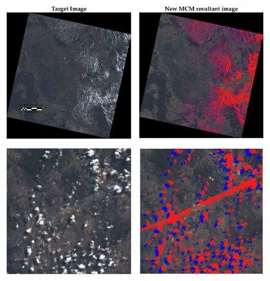
Cloud-shadow masking in the tropical area (Bulawayo, Zimbabwe). (a) A target image, (b) The new MCM resultant image, (c) The previous MCM resultant image, (d) A part of the target image, (e) The new MCM resultant image of (d), and (f) The previous MCM resultant image of (d), respectively. The red and blue color indicates cloud and the cloud-shadow region, respectively.
Figure 10.
Cloud-shadow masking in the tropical area (Bulawayo, Zimbabwe). (a) A target image, (b) The new MCM resultant image, (c) The previous MCM resultant image, (d) A part of the target image, (e) The new MCM resultant image of (d), and (f) The previous MCM resultant image of (d), respectively. The red and blue color indicates cloud and the cloud-shadow region, respectively.

Figure 11.
Comparison of the new MCM algorithm results and the L8 CCA algorithm results in one of the sub-tropical south images (Toowoomba, Queensland, Australia). The red and blue color indicates cloud and the cloud-shadow region, respectively.
Figure 11.
Comparison of the new MCM algorithm results and the L8 CCA algorithm results in one of the sub-tropical south images (Toowoomba, Queensland, Australia). The red and blue color indicates cloud and the cloud-shadow region, respectively.

Figure 12.
The results of the new MCM and L8 CCA in the detection of cloud and cloud-shadow in (a) settlement, (b) cropland, (c) forest, and (d) desert for statistical assessments.
Figure 12.
The results of the new MCM and L8 CCA in the detection of cloud and cloud-shadow in (a) settlement, (b) cropland, (c) forest, and (d) desert for statistical assessments.

Figure 13.
Comparison between the MCM and L8 CCA algorithm in the accuracy of the cloud-masking results.
Figure 13.
Comparison between the MCM and L8 CCA algorithm in the accuracy of the cloud-masking results.

Figure 14.
Comparison between the MCM and L8 CCA algorithm in the accuracy of the cloud-shadow masking results.
Figure 14.
Comparison between the MCM and L8 CCA algorithm in the accuracy of the cloud-shadow masking results.


Table 1.
Cloud types identified visually (adapted from [14]).
Table 1.
Cloud types identified visually (adapted from [14]).
| Genus | Height | The Height of Cloud Base | ||
|---|---|---|---|---|
| Polar Regions | Temperate Regions | Tropical Regions | ||
 | ||||
| Low | Below 2 km | Below 2 km | Below 2 km | |
 | ||||
| Middle | 2–4 km | 2–7 km | 2–8 km | |
 | ||||
| Height | 3–8 km | 5–13 km | 6–18 km | |
Table 2.
Selected Landsat 8 images with path/row, area, environment types, cloud types, and surface cover features.
Table 2.
Selected Landsat 8 images with path/row, area, environment types, cloud types, and surface cover features.
| Path/Row | Area | Environment | Cloud Type | Land Cover Class |
|---|---|---|---|---|
| 090/079 | Queensland, Australia | Sub-tropical South | Thick | Settlement, crop land, forest, wetland, and open land |
| 091/085 | New South Wales, Australia | Sub-tropical South | Thick | Settlement, cropland, forest, wetland, open land, and water |
| 091/085 | New South Wales, Australia | Sub-tropical South | Thin | Settlement, cropland, forest, wetland, open land, and water |
| 170/078 | Johannesburg, South Africa | Sub-tropical South | Thick | Settlement, cropland, open land, and water |
| 171/074 | Bulawayo, Zimbabwe | Tropical | Thick and thin | Settlement, cropland, forest, open land, swamp, and water |
| 175/062 | Kindu—Democratic Republic of The Congo | Tropical | Thick | Settlement, open land, cropland, forest, water |
| 170/063 | Tabora, Tanzania | Tropical | Thick | Open land, wet land, forest and water |
| 041/033 | Nevada, USA | Sub-tropical North | Thick | Settlement, open land, and water |
| 192/024 | Berlin, Germany | Sub-tropical North | Thick | Settlement, cropland, forest, open land, and water |
| 202/038 | Marrakesh, Morocco | Sub-tropical North | Thick | Settlement, desert, cropland, open land, and water |
Table 3.
The results of commission error and omission error of cloud masking using the new MCM algorithm.
Table 3.
The results of commission error and omission error of cloud masking using the new MCM algorithm.
| Settlement | Cropland | Forest | Desert | Average | |
|---|---|---|---|---|---|
| Commission Error of New MCM | 0.024 | 0.018 | 0.035 | 0.001 | 0.019 |
| Commission Error of L8 CCA | 0.013 | 0.004 | 0.006 | 0.003 | 0.007 |
| Omission Error of New MCM | 0.009 | 0.039 | 0.120 | 0.009 | 0.010 |
| Omission Error of L8 CCA | 0.220 | 0.212 | 0.126 | 0.500 | 0.264 |
Table 4.
The results of commission error and omission error of cloud-shadow masking using the new MCM algorithm.
Table 4.
The results of commission error and omission error of cloud-shadow masking using the new MCM algorithm.
| Settlement | Cropland | Forest | Desert | Average | |
|---|---|---|---|---|---|
| Commission Error of New MCM | 0.013 | 0.010 | 0.058 | 0.000 | 0.020 |
| Commission Error of L8 CCA | 0.583 | 0.339 | 0.354 | 0.165 | 0.360 |
| Omission Error of New MCM | 0.025 | 0.024 | 0.001 | 0.084 | 0.033 |
| Omission Error of L8 CCA | 0.136 | 0.104 | 0.043 | 0.249 | 0.133 |
© 2019 by the authors. Licensee MDPI, Basel, Switzerland. This article is an open access article distributed under the terms and conditions of the Creative Commons Attribution (CC BY) license (http://creativecommons.org/licenses/by/4.0/).
Share and Cite
MDPI and ACS Style
Candra, D.S.; Phinn, S.; Scarth, P. Automated Cloud and Cloud-Shadow Masking for Landsat 8 Using Multitemporal Images in a Variety of Environments. Remote Sens. 2019, 11, 2060. https://0-doi-org.brum.beds.ac.uk/10.3390/rs11172060
AMA Style
Candra DS, Phinn S, Scarth P. Automated Cloud and Cloud-Shadow Masking for Landsat 8 Using Multitemporal Images in a Variety of Environments. Remote Sensing. 2019; 11(17):2060. https://0-doi-org.brum.beds.ac.uk/10.3390/rs11172060
Chicago/Turabian StyleCandra, Danang Surya, Stuart Phinn, and Peter Scarth. 2019. "Automated Cloud and Cloud-Shadow Masking for Landsat 8 Using Multitemporal Images in a Variety of Environments" Remote Sensing 11, no. 17: 2060. https://0-doi-org.brum.beds.ac.uk/10.3390/rs11172060
Note that from the first issue of 2016, this journal uses article numbers instead of page numbers. See further details here.