Global Ionospheric Model Accuracy Analysis Using Shipborne Kinematic GPS Data in the Arctic Circle

Abstract

The global ionospheric model built by the International Global Navigation Satellite System (GNSS) Service (IGS) using GNSS reference stations all over the world is currently the most widely used ionospheric product on a global scale. Therefore, analysis and evaluation of this ionospheric product’s accuracy and reliability are essential for the practical use of the product. In contrast to the traditional way of assessing global ionospheric models with ground-based static measurements, our study used shipborne kinematic global positioning system (GPS) measurements collected over 18 days to perform a preliminary analysis and evaluation of the accuracy of the global ionospheric models; our study took place in the Arctic Circle. The data from the International GNSS Service stations near the Arctic Circle were used to verify the ionospheric total electron contents derived from the kinematic data. The results suggested that the global ionospheric model had an approximate regional accuracy of 12 total electron content units (TECu) within the Arctic Circle and deviated from the actual ionospheric total electron content value by about 4 TECu.

1. Introduction

As an important component of the solar–terrestrial environment, the ionosphere has profound effects on modern radio engineering and human activities. Studying the ionosphere allows us to better understand the ionosphere itself, search for ways to overcome its potential harms, and determine methods to utilize it for our benefit. In addition, it also helps promote the study and development of earth science-related ionosphere theories and applications [1]. Many international studies have proved the potential harm of the ionosphere, the most significant of which is the impact on navigation accuracy [2,3,4,5]. Therefore, understanding the ionosphere will also promote the development of navigation and positioning technology [6,7]. The invention and rapid development of the Global Navigation Satellite System (GNSS) resulted in it becoming the main technique for ionosphere observation, as it is continuous, comprehensive, low-cost, highly accurate, and can be utilized in all types of weather [7,8,9,10,11,12,13,14,15,16].

The International GNSS Service (IGS) has been using the continuously operating GNSS reference stations around the world to develop a global ionospheric model, which has become one of the most important tools for ionosphere research and applications [17]. Therefore, analyzing and evaluating the accuracy and reliability of the IGS ionospheric product is essential for its proper use. Restricted by its ground-based observation stations, it was previously shown that the global ionospheric model published by the IGS had a lower accuracy over the sea compared to that over the land [18,19,20,21]. Although there have been some researchers who have used satellites for ocean altimetry to analyze and model the ionospheric total electron content (TEC) over the sea [22,23,24], due to inevitable systematic errors between different data sources and a limited number of existing satellites, the accuracy of the product is low. Compared to that in low-latitude and mid-latitude regions, the ionospheric structure in the polar regions is more complicated and volatile [25]. This special structure of the ionosphere makes the changing pattern of the TEC unpredictable, thereby causing the global ionospheric model to demonstrate a lower accuracy in polar regions than in low-latitude and mid-latitude regions [26]. This is particularly true in the Arctic Circle, due both to a lack of observational data from global positioning system (GPS) reference stations as well as more complicated ionospheric characteristics. Some scholars have used traditional ground-based stations to study the characteristics and effects of the Arctic ionosphere [27,28,29]. However, they could not reflect the situation well without high spatial and temporal resolution data. Therefore, analyzing and evaluating the accuracy of the global ionospheric model in the Arctic Circle is crucial for the proper application of the IGS ionospheric products in that region and related work in the future.

In our study, GNSS receivers were installed on a Chinese research vessel for an annual Arctic research expedition, which provided invaluable data for our purposes. Our study assessed the accuracy of the global ionospheric model in the Arctic Circle quantitatively using the data collected in September 2017. For many years, the IGS has been acquiring ionosphere information from the continuously operating GNSS reference stations around the world. In 1998, it approved and started implementing the TEC Ionosphere Exchange Format (IONEX) [17], which has become an important component of the IGS products and has provided abundant fundamental data for ionospheric studies around the world.

Among the four ionospheric analysis centers of the IGS, the Center for Orbit Determination in Europe and the European Space Agency modeled the global ionospheric TEC with the spherical harmonic method [30,31]. By adopting a holistic modeling approach, this method presented an effective extrapolation for the ionospheric TEC and demonstrated a certain accuracy in computing the ionospheric TEC for regions without direct observational data. However, this method failed to show the subtle changes in the regional ionospheric TEC. Alternatively, the Jet Propulsion Laboratory and Polytechnical University of Catalonia modeled the global ionospheric TEC based on global triangular grids and the model interpolation of selected reference stations, respectively [31,32]. These methods were able to effectively show the subtle changes in the ionospheric TEC of the observation region but failed to reasonable extrapolate ionospheric TEC outside the region. In addition, they generally relied on empirical models (such as the international reference ionosphere model) or mathematical interpolation (such as linear and Kriging interpolation) such that their accuracies cannot be guaranteed.

Based on some previous studies [30,31,32], the spherical harmonic method works relatively well for the interpolation and extrapolation of ionospheric TEC on a global scale and maintains the continuity and reliability of ionospheric TEC changes more effectively. Therefore, the global ionospheric model built with the spherical harmonic method was chosen for our study, and the ionospheric TEC was measured with the GPS data collected in the Arctic Circle to assess the model.

The second part of this paper introduces the details about the adopted data and methods in this study. The third part outlines the results of the accuracy assessment. The fourth part summarizes the major findings and contributions of the study and identifies a direction for future investigations.

2. Mathematic Models, Data Sets, and Analysis Methods

The spherical harmonic model of the global ionospheric TEC is described as [10]:

$$VTEC(\phi ,\lambda )={\displaystyle \sum _{n=0}^{n_{d\mathit{max}}}{\displaystyle \sum _{m=0}^n\widetilde{P_{nm}}}}(\sin \phi )\cdot \left(\widetilde{A_{nm}}\cos (m\lambda )+\widetilde{B_{nm}}\sin (m\lambda )\right)$$

(1)

where $VTEC(\phi ,\lambda )$ represents the vertical TEC (VTEC) at the intersect pierce point (IPP;$(\phi ,\lambda )$); $\phi$ and $\lambda$ represent the latitude and longitude of the ionospheric IPP, respectively; $n_{d\max }$ represents the maximum degree in spherical harmonics; $\widetilde{P_{\mathrm{nm}}}(\sin \phi )=MC(n,m)\cdot P_{nm}(\sin \phi )$ represents the normalized Legendre function with the n^th degree and the m^th order; $MC(n,m)$ represents the normalized function shown in Equation (2) below; and $\widetilde{A_{nm}}$ and $\widetilde{B_{nm}}$ represent parameters in the model that are to be estimated:

$$MC\left(n,m\right)=\sqrt{(n-m)!(2n+1)(2-{\delta }_{0m})/(n+m)!}$$

(2)

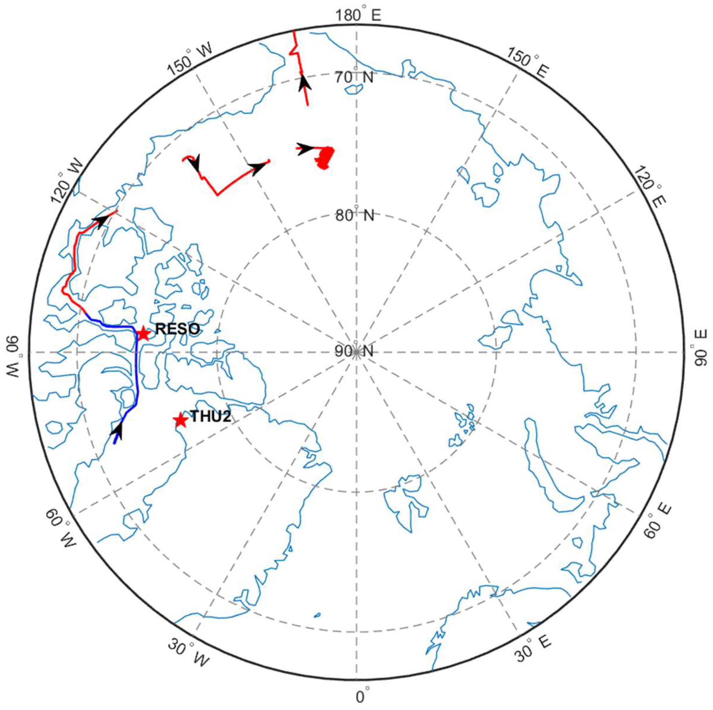
2.1. Shipborne Kinematic GPS Data from the Arctic Research Expeditions

In 2017, a GNSS monitoring receiver set was brought onboard a Chinese research vessel operating in the Arctic region. The receiver Trimble NetR9 was used together with an antenna called TRM57971.00. The receiver was used to track GPS signals and transmit data, including pseudo-range (C1C, C2W) and carrier-phase measurements (L1C, L2W). The actual route of the Chinese research vessel was in the area between 66°N and 77°N. The sailing time was from September 1 to 22, 2017 (the data for September 6, 10, 16, and 20 was missing). The ionospheric TEC information on the satellite signal path was gathered from the dual-frequency data received by the receiver. This information formed the basis of the accuracy and reliability assessment for the global ionospheric model in the Arctic Circle.

The data from the IGS GNSS reference stations (RESO and THU2) near the Arctic Circle for September 1 to 3, 2017 were collected to verify the reliability of the shipborne kinematic GPS measurements. The actual route taken by the Chinese research vessel for its operation within the Arctic Circle and the location of IGS GNSS reference stations are shown in Figure 1.

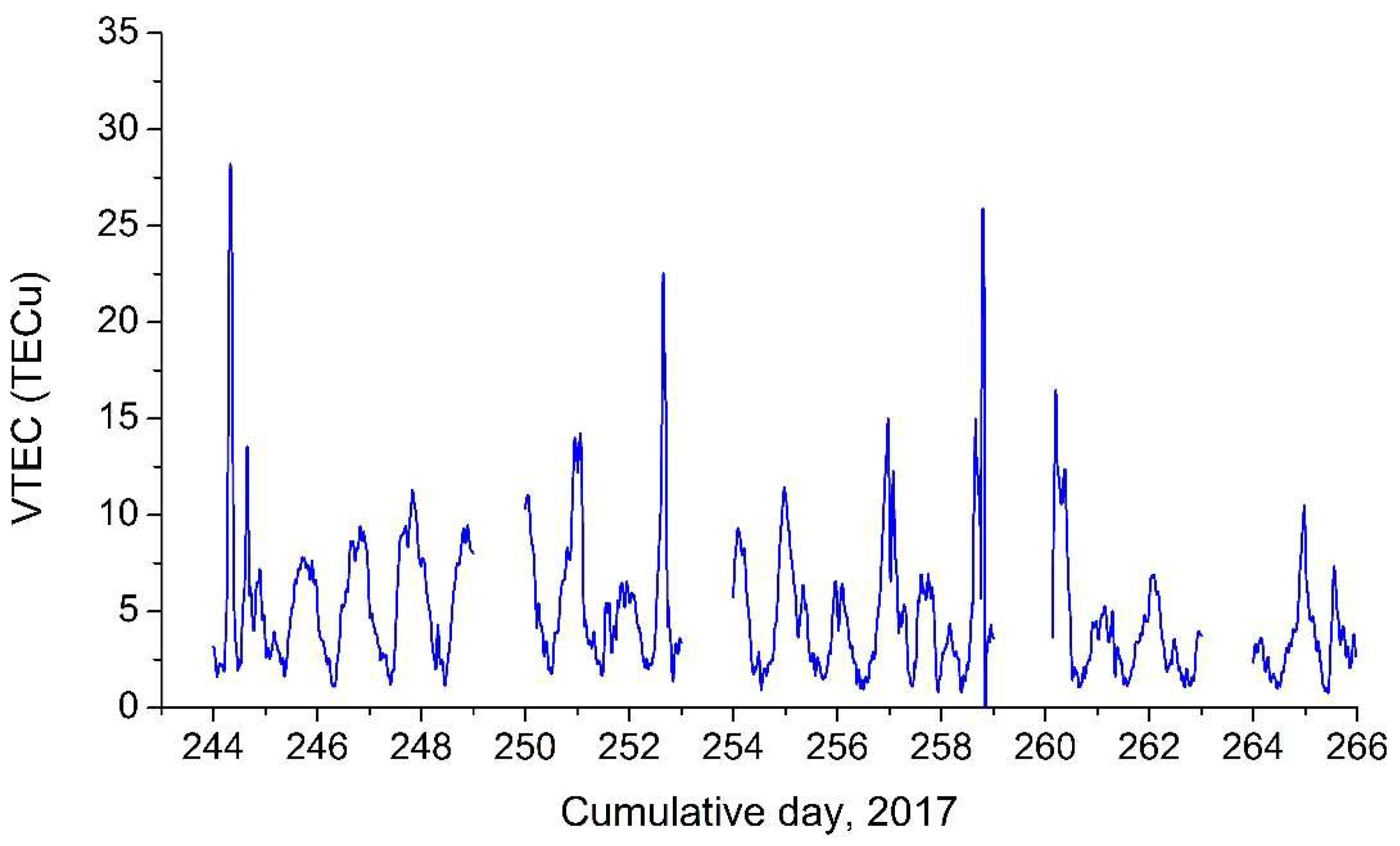
2.2. Ionospheric TEC Information Extracted from Dual-Frequency GPS Data

GPS data can be classified into code-phase and carrier-phase measurements. As the code pseudo-range has a lower accuracy, information about the absolute TEC of the ionosphere that is obtained using the code pseudo-range alone usually has a low accuracy as well [33,34]. Alternatively, due to the inclusion of integer-ambiguity parameters for two frequencies, the carrier-phase measurement can only obtain information about the relative TEC of the ionosphere [35].

To acquire highly accurate information about the absolute TEC of the ionosphere, this study adopted the carrier-phase smoothed pseudo-range method and extracted the ionospheric TEC information from the dual-frequency GPS data. The function expression is given as follows [17]:

$$P_1-P_2=\frac{40.3(f_2^2-f_1^2)}{f_1^2{f}_2^2}\text{·}F(\alpha )\text{·}VTEC+c(DC{B}_s+DC{B}_r)$$

(3)

where $P_1$ and $P_2$ represent the values of the code pseudo-ranges at different frequencies; $f_1$ and $f_2$ represent the frequencies corresponding to carrier signals $L_1$ and $L_2$, respectively; $F(\alpha )$ represents the projection function, which can convert the ionospheric TEC value in the ionospheric IPP direction into the ionospheric VTEC value at that point (the function mainly depends on the relative zenith distance $\alpha$ between the satellite and the ionospheric IPP); $c$ represents the speed of light in a vacuum; and $DC{B}_s$ and $DC{B}_r$ represent the difference code biases (DCBs) of the satellite and the receiver, respectively.

Therefore, from the equation above, highly accurate absolute TEC information from the ionosphere can be obtained after determining the DCB in the satellite and the receiver.

2.3. Estimation of Kinematic GPS-Difference Code Biases of the Receiver

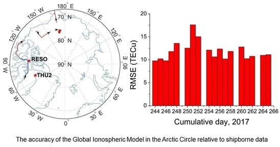
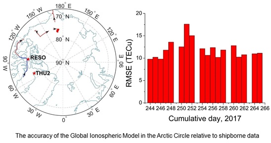
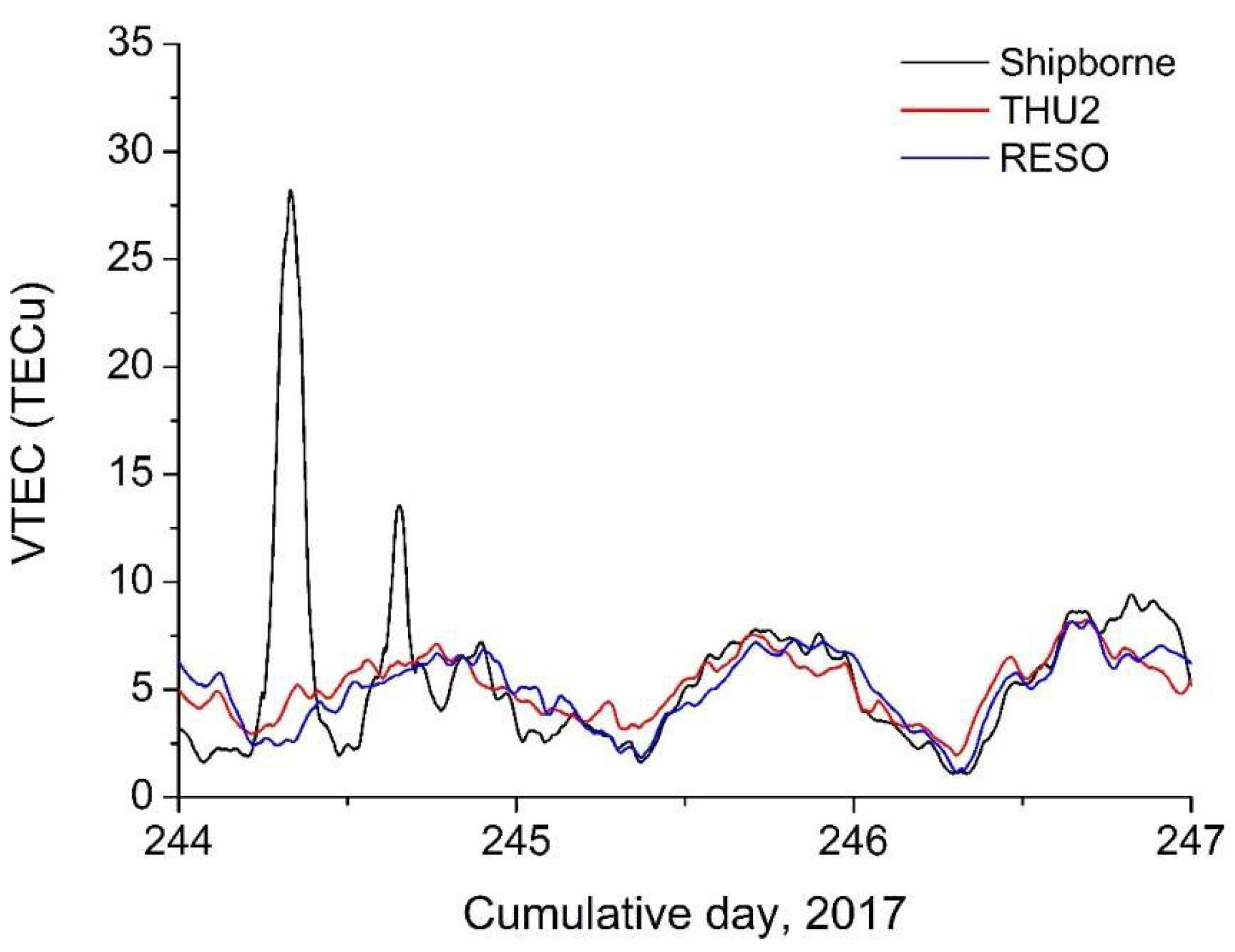
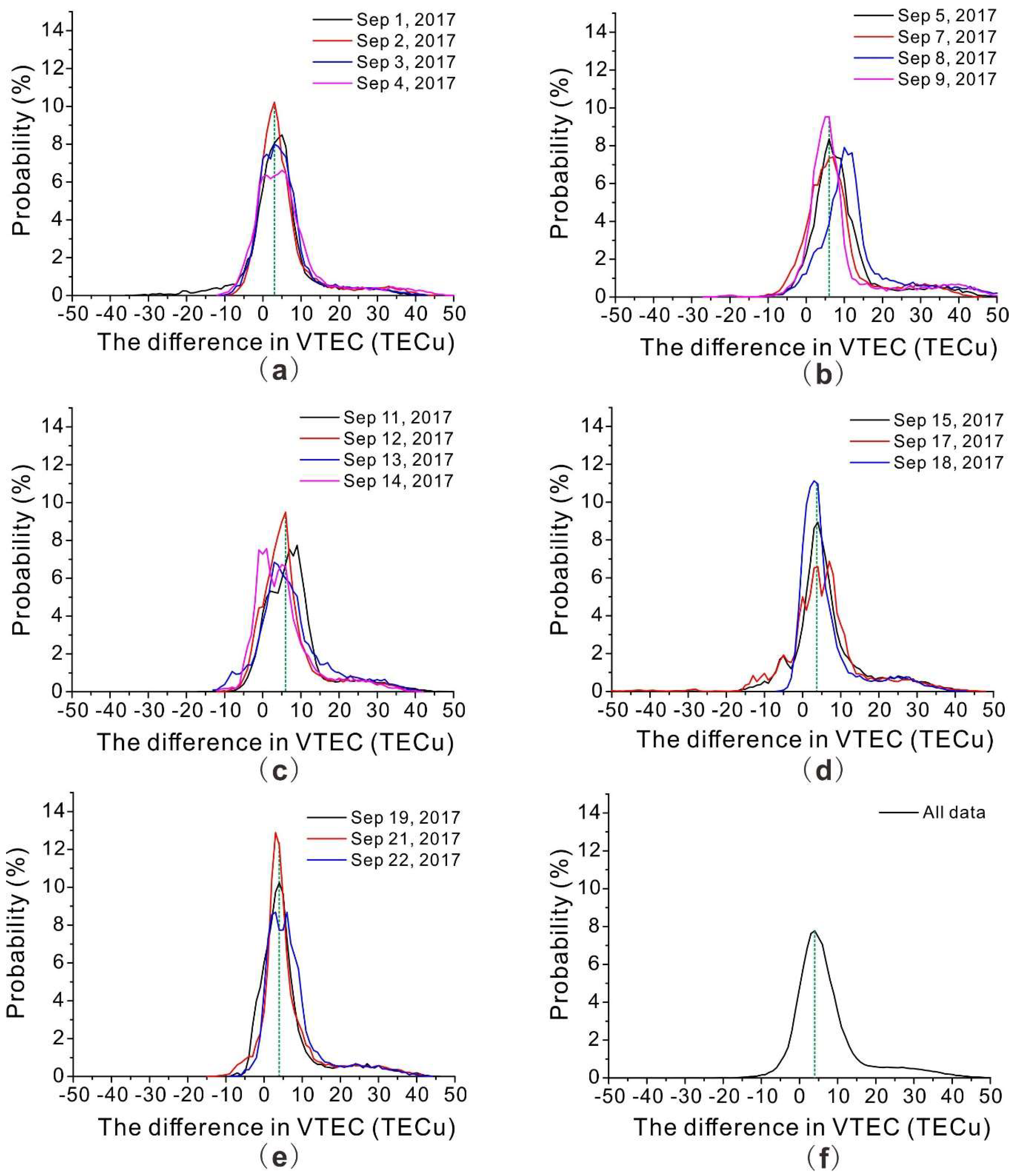
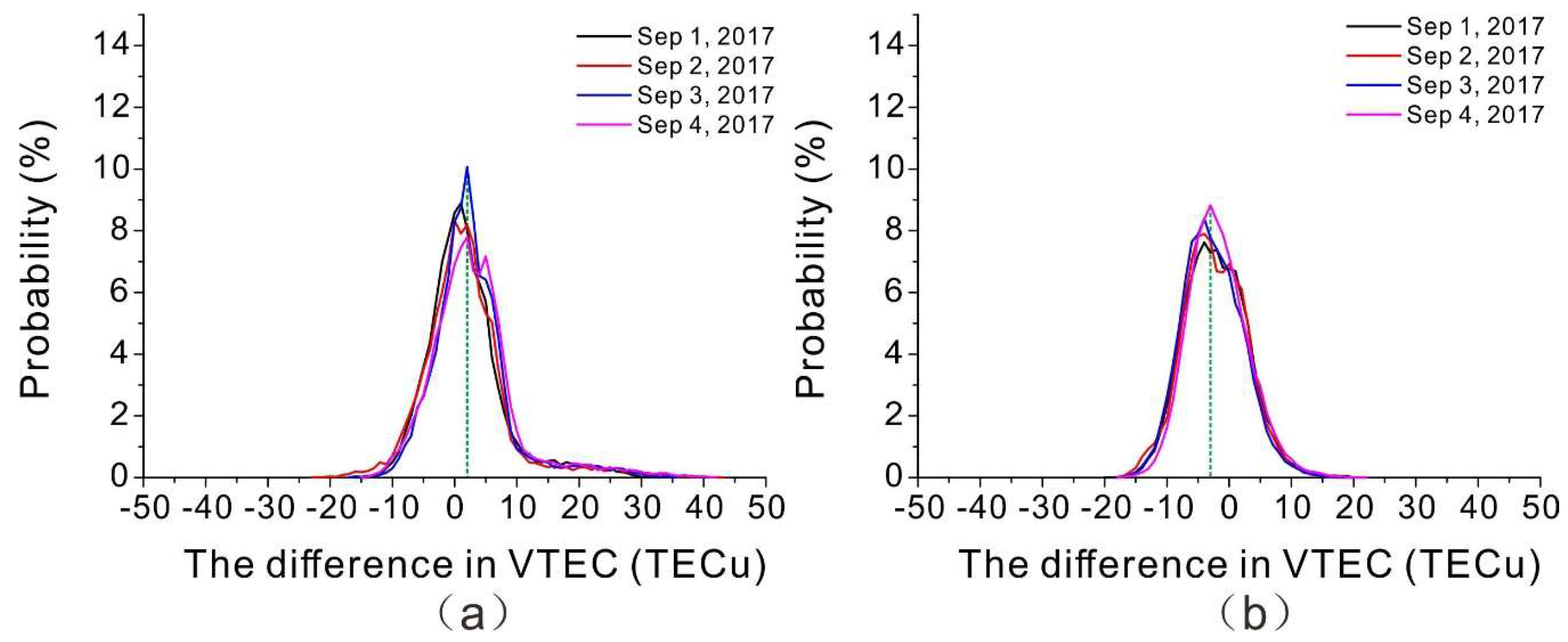
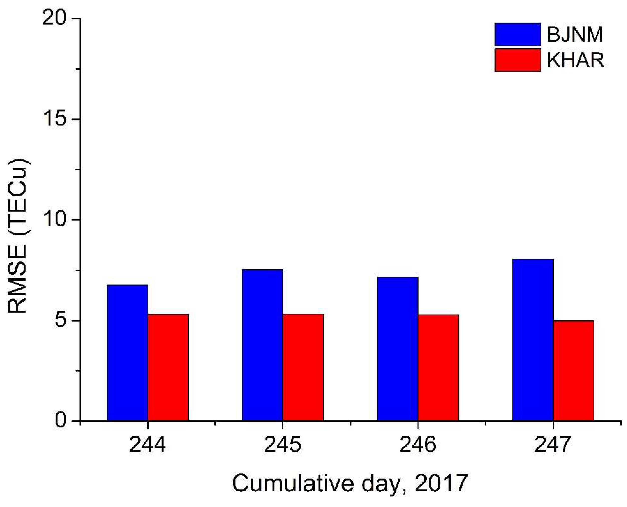
DCBs in the satellite and the receiver are significant errors in the ionospheric TEC calculation. While DCB in the satellite can be corrected using IGS products, DCB in the receiver can be estimated accurately only with its own observational data. Unlike the IGS, which estimates DCB simultaneously when modeling the global ionospheric model, we describe the trend of changes in the ionosphere above the kinematic GPS monitoring stations with a generalized trigonometric series [35], with the DCB of the receiver for one day estimated as a constant. The model, using a generalized trigonometric series, considers both the gradient of regional changes [36,37] and the cyclic nature of the ionosphere for one day, it is therefore more suitable for the accurate simulation of the ionospheric delay occurring above the kinematic GPS reference stations. The model using the generalized trigonometric series is shown as:

$$VTEC\left(\phi ,h\right)={\displaystyle \sum _{n=0}^{n_{max}}{\displaystyle \sum _{m=0}^{m_{max}}\left\{E_{nm}{\left(\phi -{\phi }_0\right)}^n{h}^m\right\}}}+{\displaystyle \sum _{k=0}^{k_{max}}\{C_k\cos (k\cdot h)}+S_k\sin (k\cdot h)\}$$

(4)

where ${\phi }_0$ represents the latitude of the center of the regional ionospheric TEC model; $h$ represents the function related to the standard time $t$ at the IPP; $n_{max},m_{max}$, and $k_{max}$ represent the maximum orders of the polynomial function and the trigonometric function, respectively; and $E_{nm},C_k,S_k$ represent the coefficients in the model that are to be estimated. Other parameters are the same as the corresponding symbols in Equation (1).

3. Results

Information about a clean absolute TEC of the ionosphere was obtained by correcting the VTEC value at the ionospheric IPP with the estimated values of DCB in the satellite and the receiver with the method discussed in Section 2.3. Taking that “clean” absolute TEC of the ionosphere as the reference, the ionospheric TEC was calculated for the corresponding time and location using the IONEX file interpolation. The direct ionospheric TEC variation is given in Figure 2. It can be seen that the irregularity of the ionosphere in the Arctic Circle makes it difficult to describe.

To prove the reliability of shipborne data, direct changes in the ionospheric TEC calculated by the shipborne data and the IGS reference stations data are compared. The results are shown in Figure 3. When the ship sailed near the IGS reference stations, the shape and magnitude of the ionospheric TECs were similar. This confirms the reliability of the shipborne data. Meanwhile, the shipboard data can reflect abnormal changes in the ionosphere in the Arctic Circle, which is more advantageous in the Arctic region where the IGS reference stations are sparse.

Then, the difference between the global ionosphere model TEC and the actual ionospheric TEC was obtained. The probability distribution of the difference is given in Figure 4. It can be seen that the overall difference between the global ionospheric model TEC and the ionospheric TEC obtained from the kinematic data is about 3 to 6 total electron content units (TECu). Overall, this deviation is about 4 TECu.

The root mean square error (RMSE) of the daily deviation was counted. This value was used to represent the accuracy of the model value relative to the measured value. The expression of RMSE is given as follows:

$$RMSE=\sqrt{\frac{{\displaystyle \sum _{\mathrm{i}=1}^N{(X_{model}-X_{shipborne})}^2}}{N}}$$

(5)

where $N$ represents the number of samples; $X_{model}$ represents the model value; and $X_{shipborne}$ represents the measured value. The results are summarized in

Table 1. The root mean square error (RMSE) of difference between the global ionospheric model TEC and the actual ionospheric TEC measured with the shipborne receiver during China’s Arctic Expedition (unit: TECu).

Day	1	2	3	4	5	7	8
RMSE	9.79	10.21	9.80	11.81	13.95	12.54	17.61
Day	9	11	12	13	14	15	17
RMSE	15.04	12.13	10.65	12.37	10.19	11.83	12.81
Day	18	19	21	22	Total
RMSE	10.25	10.77	10.98	11.12	12.02

with the corresponding dates of observation. The last item in the table denotes the overall accuracy during the measurement period. The result is shown in Figure 5. During the test, the highest accuracy was observed on September 1, and the worst accuracy was observed on September 8. The overall accuracy was approximately 12 TECu.

The data from the IGS GNSS reference stations BJNM (40.2453°N; 116.2241°E, geographic) and KHAR (50.0051°N; 36.2390°E, geographic) for September 1 to 4, 2017, were used to evaluate the accuracy of the global ionospheric model in other latitude regions. The probability distribution and the RMSE of the difference are shown in Figure 6 and Figure 7, respectively. The global ionospheric model had an accuracy of 6 TECu and a deviation of 3 TECu in regions where IGS GNSS reference stations are intensively distributed. Compared with the results of the Arctic Circle, it is again illustrated that the global ionospheric model performs worse in the Arctic Circle.

4. Conclusions

The global ionospheric model from the IGS generally has a relatively low accuracy when used in the polar regions, and it is often difficult to obtain a reliable assessment of the accuracy of the ionospheric products in that region with the existing ground-based GNSS observation stations. In this study, using the shipborne kinematic GPS data from a Chinese Arctic expedition, the DCB values were accurately estimated with a model based on a generalized trigonometric series; these values were then used to perform a detailed assessment of the accuracy and reliability of the global ionospheric model; our study was conducted in the Arctic Circle.

The data from IGS reference stations near the Arctic Circle were used to verify the ionospheric total electron content from the shipborne kinematic GPS measurements. The assessment results indicated that the TEC from the kinematic GPS measurements is reliable, and the overall difference between the global ionospheric model TEC and the actual ionospheric TEC is about 3 to 6 TECu in the Arctic Circle. Further, the accuracy of the global ionospheric model was approximately 12 TECu in the region.

For a better assessment of the accuracy and reliability of the global ionospheric model in the Arctic Circle, future work has been designed to collect and analyze GNSS data acquired from the multi-GNSS receivers on board an Arctic research vessel to extend the scope of the ionospheric model assessment with more data sets.

References

1. Yuan, Y. Study on Theories and Methods of Correcting Ionospheric Delay and Monitoring Ionosphere Based on GPS. Ph.D. Dissertation, Institute of Geodesy and Geophysics Chinese Academy of Sciences, the Graduate School of the Chinese Acadmy of Science, Wuhan, China, May 2002. [Google Scholar]
2. Kim, E.; Walter, T.; Powell, J. Adaptive carrier smoothing using code and carrier divergence. Proc. ION NTM 2007, January, 22–24. [Google Scholar]
3. Pi, X.; Iijima, B.; Lu, W. Effects of Ionospheric Scintillation on GNSS-Based Positioning. J. Inst. Navig. 2017, 64, 3–22. [Google Scholar] [CrossRef]
4. Lee, J.; Morton, Y.; Lee, J.; Moon, H.; Seo, J. Monitoring and Mitigation of Ionospheric Anomalies for GNSS-Based Safety Critical Systems: A review of up-to-date signal processing techniques. IEEE Signal Process. Mag. 2017, 34, 96–110. [Google Scholar] [CrossRef]
5. Park, B.; Lim, C.; Yun, Y.; Kim, E.; Kee, C. Optimal Divergence-Free Hatch Filter for GNSS Single-Frequency Measurement. Sensors 2017, 17, 448. [Google Scholar] [CrossRef] [PubMed]
6. Yuan, Y.; Ou, J. An Improvement To Ionospheric Delay Correction For Single Frequency GPS user—the APR-I Scheme. J. Geodesy 2001, 75, 331–336. [Google Scholar] [CrossRef]
7. Yuan, Y.; Wang, N.; Li, Z.; Huo, X. The BeiDou Global Broadcast Ionospheric Delay Correction Model (BDGIM) and Its Preliminary Performance Evaluation Results. NAVIGATION 2019, 66, 55–69. [Google Scholar] [CrossRef]
8. Lanyi, G.; Roth, T. A comparison of mapped and measured total ionospheric electron content using global positioning system and beacon satellite observations. Radio Sci. 1988, 23, 483–492. [Google Scholar] [CrossRef]
9. Mannucci, A.; Wilson, B.; Yuan, D.; Ho, C.; Lindqwister, U.; Runge, T. A global mapping technique for GPS-derived ionospheric total electron content measurements. Radio Sci. 1998, 33, 565–582. [Google Scholar] [CrossRef]
10. Schaer, S. Mapping and Predicting the Earth’s Ionosphere Using the Global Positioning System. Ph.D. Thesis, Astronomical Institute, University of Berne, Bern, Switzerland, 1999. [Google Scholar]
11. Yuan, Y.; Ou, J. Auto-Covariance Estimation of Variable Samples (ACEVS) and Its Application for Monitoring Random Ionosphere Using GPS. J. Geodesy 2001, 75, 438–447. [Google Scholar] [CrossRef]
12. Feltens, J. Development of a new three-dimensional mathematical ionosphere model at European space agency/European space operations centre. Space Weather 2007, 5, 1–17. [Google Scholar] [CrossRef]
13. Yuan, Y.; Huo, X.; Ou, J. Models and Methods for precise determination of ionospheric delays using GPS. Prog. Nat. Sci. 2007, 17, 187–196. [Google Scholar] [CrossRef]
14. Dyrud, L.; Jovancevic, A.; Brown, A.; Wilson, D.; Ganguly, S. Ionospheric measurement with GPS. Radio Sci. 2008, 43, 4159–5165. [Google Scholar] [CrossRef]
15. Yuan, Y.; Tscherning, C.; Knudsen, P.; Xu, G.; Ou, J. The ionospheric eclipse factor method (IEFM) and its application to determining the ionospheric delay for GPS. J. Geodesy 2008, 82, 1–8. [Google Scholar] [CrossRef]
16. Ke, F.; Wang, J.; Tu, M.; Wang, X.; Wang, X.; Zhao, X.; Deng, J. Morphological characteristics and coupling mechanism of the ionospheric disturbance caused by Super Typhoon Sarika in 2016. Adv. Space Res. 2018, 62, 1137–1145. [Google Scholar] [CrossRef]
17. Wang, C.; Shi, C.; Fan, L.; Zhang, H. Improved Modeling of Global Ionospheric Total Electron Content Using Prior Information. Remote Sens. 2018, 10, 63. [Google Scholar] [CrossRef]
18. Mannucci, A.; Iijima, B.; Lindqwister, U.; Pi, X.; Sparks, L.; Wilson, B. GPS and Ionosphere: Review of Radio Science 1996-1999; Oxford Univ. Press: New York, NY, USA, 1999. [Google Scholar]
19. Hernández-Pajares, M. Performance of IGS Ionosphere TEC Maps; Technical University of Catalonia: Barcelona, Spain, 2003. [Google Scholar]
20. Hernández-Pajares, M. IGS Ionosphere WG Status Report: Performance of IGS Ionosphere TEC Maps; IGS Workshop: Bern, Switzerland, 2004. [Google Scholar]
21. Luo, X.; Xu, H.; Li, Z.; Zhang, T.; Gao, J.; Shen, Z.; Yang, C.; Wu, Z. Accuracy assessment of the global ionospheric model over the Southern Ocean based on dynamic observation. J. Atmos. Sol. Terr. Phys. 2017, 154, 127–131. [Google Scholar] [CrossRef]
22. Dettmering, D.; Limberger, M.; Schmidt, M. Using DORIS measurements for modeling the vertical total electron content of the Earth’s ionosphere. J. Geod. 2014, 88, 1131–1143. [Google Scholar] [CrossRef]
23. Brunini, C.; Meza, A.; Bosch, W. Temporal and spatial variability of the bias between TOPEX- and GPS-derived total electron content. J. Geod. 2005, 79, 175–188. [Google Scholar] [CrossRef]
24. Chen, P.; Yao, W.; Zhu, X. Combination of Ground- and Space-Based Data to Establish a Global Ionospheric Grid Model. IEEE Trans. Geosci. Remote Sens. 2014, 53, 1073–1081. [Google Scholar] [CrossRef]
25. Meng, Y.; Wang, Z.M. Research of Polar TEC fluctuations and polar patches during magnetic storm using GPS. Chin. J. Geophy. 2008, 51, 17–24. [Google Scholar]
26. Liu, Y.; Wang, J.; Zhang, C. Study of GNSS Loss of Lock Characteristics under Ionosphere Scintillation with GNSS Data at Weipa (Australia) During Solar Maximum Phase. Sensors 2017, 17, 2205. [Google Scholar] [CrossRef] [PubMed]
27. Mitchell, C.; Alfonsi, L.; De Franceschi, G.; Lester, M.; Romano, V.; Wernik, A. GPS TEC and scintillation measurements from the polar ionosphere during the October 2003 storm. Geophys. Res. Lett. 2005, 32, L12S03. [Google Scholar] [CrossRef]
28. Jayachandran, P.; Langley, R.; MacDougall, J.; Mushini, S.; Pokhotelov, D.; Hamza, A.; Mann, I.; Milling, D.; Kale, Z.; Chadwick, R.; et al. Canadian High Arctic Ionospheric Network (CHAIN). Radio Sci. 2009, 44, 1. [Google Scholar] [CrossRef]
29. El-Arini, M.; Secan, J.; Klobuchar, J.; Doherty, P.; Bishop, G.; Groves, K. Ionospheric effects on GPS signals in the Arctic region using early GPS data from Thule, Greenland. Radio Sci. 2009, 44, 1–14. [Google Scholar] [CrossRef]
30. Feltens, J. The International GPS Service (IGS) ionosphere working group. Adv. Space Res. 2003, 31, 205–214. [Google Scholar] [CrossRef]
31. Hernández-Pajares, M.; Juan, J.; Sanz, J.; Orus, R.; Garcia-Rigo, A.; Feltens, J.; Komjathy, A.; Schaer, S.; Krankowski, A. The IGS VTEC maps: A reliable source of ionospheric information since 1998. J. Geod. 2009, 83, 263–275. [Google Scholar] [CrossRef]
32. Mannucci, A.; Wilson, B.; Edwards, C. A new method for monitoring the Earth ionosphere total electron content using the GPS global network. In Proceedings of the 1993 ION GPS-93, Salt Lake City, UT, USA, 22–24 September 1993. [Google Scholar]
33. Lee, C.; Lee, D.; Chung, N.; Chang, I.; Kawai, E.; Takahashi, F. Development of a GPS Codeless Receiver for Ionospheric Calibration and Time Transfer. IEEE Trans. Instrum. Meas. 1993, 42, 494–497. [Google Scholar] [CrossRef]
34. Caciotta, M.; Leccese, F.; Piuzzi, E. Study of a new GPS-carriers based time reference with high instantaneous accuracy. In Proceedings of the 2007 8th International Conference on Electronic Measurement and Instruments, Xian, China, 16–18 August 2007; pp. 11–14. [Google Scholar] [CrossRef]
35. Li, Z.; Yuan, Y.; Li, H.; Ou, J.; Huo, X. Two-step method for the determination of the differential code biases of COMPASS satellites. J. Geod. 2012, 86, 1059–1076. [Google Scholar] [CrossRef]
36. Yuan, Y.; Ou, J. A generalized trigonometric series function model for determining ionospheric delay. Prog. Nat. Sci. 2004, 14, 1010–1014. [Google Scholar] [CrossRef]
37. Li, Z.; Yuan, Y.; Wang, N.; Hernández-Pajares, M.; Huo, X. SHPTS: Towards a new method for generating precise global ionospheric TEC map based on spherical harmonic and generalized trigonometric series functions. J. Geod. 2015, 89, 331–345. [Google Scholar] [CrossRef]
Figure 1. The route of the Chinese research vessel within the Arctic Circle and the location of the ground-based Global Navigation Satellite System (GNSS) reference stations. The days near the International GNSS Service (IGS) stations are shown as a blue line (September 1 to 3, 2017).
Remotesensing 11 02062 g001
Figure 2. The direct ionospheric total electron content (TEC) variation in shipborne data.
Remotesensing 11 02062 g002
Figure 3. Comparison between Vertical TEC (VTEC) changes in shipborne data and in the IGS reference stations data.
Remotesensing 11 02062 g003
Figure 4. The probability distribution of the differences between the global ionosphere model TEC and ionospheric TEC obtained from the kinematic data (a): September 1, 2, 3, and 4; (b): September 5, 7, 8, and 9; (c): September 11, 12, 13, and 14; (d): September 15, 17, and 18; (e): September 19, 21, and 22; (f): Total data). TECu = total electron content units.
Remotesensing 11 02062 g004
Figure 5. The RMSE of the difference between the global ionospheric model TEC and the ionospheric TEC obtained from the kinematic data.
Remotesensing 11 02062 g005
Figure 6. The probability distribution of the differences between the global ionosphere model TEC and ionospheric TEC obtained from the IGS GNSS reference stations data ((a): BJNM; (b): KHAR).
Remotesensing 11 02062 g006
Figure 7. The RMSE of the difference between the global ionospheric model TEC and the ionospheric TEC obtained from the IGS GNSS reference stations data.
Remotesensing 11 02062 g007