Spatiotemporal Characterization of Mangrove Phenology and Disturbance Response: The Bangladesh Sundarban


Lamont Doherty Earth Observatory, Columbia University, Palisades, NY 10964, USA
*
Author to whom correspondence should be addressed.
Remote Sens. 2019, 11(17), 2063; https://0-doi-org.brum.beds.ac.uk/10.3390/rs11172063
Submission received: 17 July 2019
/
Revised: 22 August 2019
/
Accepted: 26 August 2019
/
Published: 2 September 2019
(This article belongs to the Section Biogeosciences Remote Sensing)
Abstract
:This work presents a spatiotemporal analysis of the phenology and disturbance response in the Sundarban mangrove forest on the Ganges-Brahmaputra Delta in Bangladesh. The methodological approach is based on an Empirical Orthogonal Function (EOF) analysis of the new Harmonized Landsat Sentinel-2 (HLS) BRDF and atmospherically corrected reflectance time series, preceded by a Robust Principal Component Analysis (RPCA) separation of Low Rank and Sparse components of the image time series. Low Rank components are spatially and temporally pervasive while Sparse components are transient and localized. The RPCA clearly separates subtle spatial variations in the annual cycle of monsoon-modulated greening and senescence of the mangrove forest from the spatiotemporally complex agricultural phenology surrounding the Sundarban. A 3 endmember temporal mixture model maps spatially coherent differences in the 2018 greening-senescence cycle of the mangrove which are both concordant and discordant with existing species composition maps. The discordant patterns suggest a phenological response to environmental factors like surface hydrology. On decadal time scales, a standard EOF analysis of vegetation fraction maps from annual post-monsoon Landsat imagery is sufficient to isolate locations of shoreline advance and retreat related to changes in sedimentation and erosion, as well as cyclone-induced defoliation and recovery.
1. Introduction
In addition to informing our understanding of forest ecology and function, mapping vegetation phenology can provide information on plants’ response to environmental influences. In situ observations of forest vegetation phenology are often expensive and time-consuming to collect – particularly in mangroves where tidal flooding and deep mud can make movement challenging. Direct observations are required to quantify flowering, fruiting and seed drop, but remotely sensed observations can provide an important complement in the form of synoptic constraints on the processes of leaf emergence, growth, and shedding. This can be especially important in biodiverse environments where phenological heterogeneity can violate simplistic assumptions about species’ response to environmental factors influencing phenology.
Most approaches to phenology mapping using remotely sensed image time series are based on some form of cyclic curve fitting (e.g., logistic function) or event detection (e.g., Start Of Season). Both of these approaches require the analyst to make assumptions about the form and magnitude of the expected phenological cycle(s). This can be particularly challenging in the presence of the spatiotemporal noise which often corrupts image time series. A partial solution is provided by characterization of the spatiotemporal variance before making the requisite assumptions. Spatiotemporal characterization of high dimensional image time series of land cover can provide a basis for the assumptions on which process models are constructed [1]. In areas where the dominant processes are well-understood, model construction can be relatively straightforward. However, in areas where processes are less well-understood or multiple processes can influence observations, it is important to characterize the observations before making the assumptions on which models are built.
This analysis focuses on mapping mangrove phenology and disturbance response in the Sundarban mangrove forest on the Ganges-Brahmaputra Delta in Bangladesh using spatiotemporal characterization and modeling of vegetation fraction [2,3,4] maps derived from the new Harmonized Landsat Sentinel-2 (HLS) BRDF and atmospherically corrected reflectance time series [5]. The Sundarban mangrove forest is the largest and most biodiverse mangrove on Earth with at least eight dominant species of tree and many minor species. The embanked islands (polders) surrounding the Sundarban are complex mosaics of single and multi-crop agriculture, forested embankments and aquaculture ponds (both seasonal and perennial). As a result, the region contains a diversity of both anthropogenic and natural vegetation phenologies. Mapping these phenologies is made more challenging by the occurrence of the southeast monsoon, imposing pervasive cloud cover between June and September. By combining Landsat and Sentinel coverage, the HLS product offers considerable improvement on earlier time series products with lower spatial, spectral and temporal resolution. The increased number of narrow NIR bands may also provide some degree of tree species discrimination while the shorter revisit time may partially offset the high frequency of tropical cloud cover. The 30 m spatial resolution offers an order of magnitude finer spatial detail than MODIS and VIIRS, and the BRDF and atmospheric corrections are also expected to reduce noise associated with temporal variability unrelated to the forest canopy.
The approach described here builds on the EOF characterization and the Temporal Mixture Modeling (TMM) approach described by Reference [1] in the context of mangrove phenology in the presence of complex multi-cropping agriculture. In the proposed extension, the spatiotemporal characterization is preceded by a Robust Principal Component Analysis (RPCA) to separate the Low Rank (L) and Sparse (S) components of the image time series and the characterization is performed on each of the L and S components separately to reduce the impact of phenological heterogeneity and cloud cover on the variance structure of the image time series. Low Rank components are spatially and temporally pervasive while Sparse components are transient and localized. Separation of these components before the EOF analysis may discriminate between dynamically distinct spatiotemporal processes which can otherwise result in coupled modes in the resulting EOF dimensions. The utility is demonstrated first on a single year time series of 25 partial cloud Sentinel-2 HLS images for the Bangladesh Sundarban. Then it is applied to a deeper time series of 69 smaller sub-tile images within the swath sidelap. In both cases, the characterization is used to identify temporal endmembers for temporal mixture models to map distinct phenologies. The results show spatially coherent patterns corresponding to phase shifts in the annual cycle of senescence and greening in the mangrove forest. Finally, a standard EOF analysis is used on a multi-decade time series of annual post-monsoon Landsat images to identify longer period changes and episodic disturbances impacting the mangrove forest.
2. Study Area
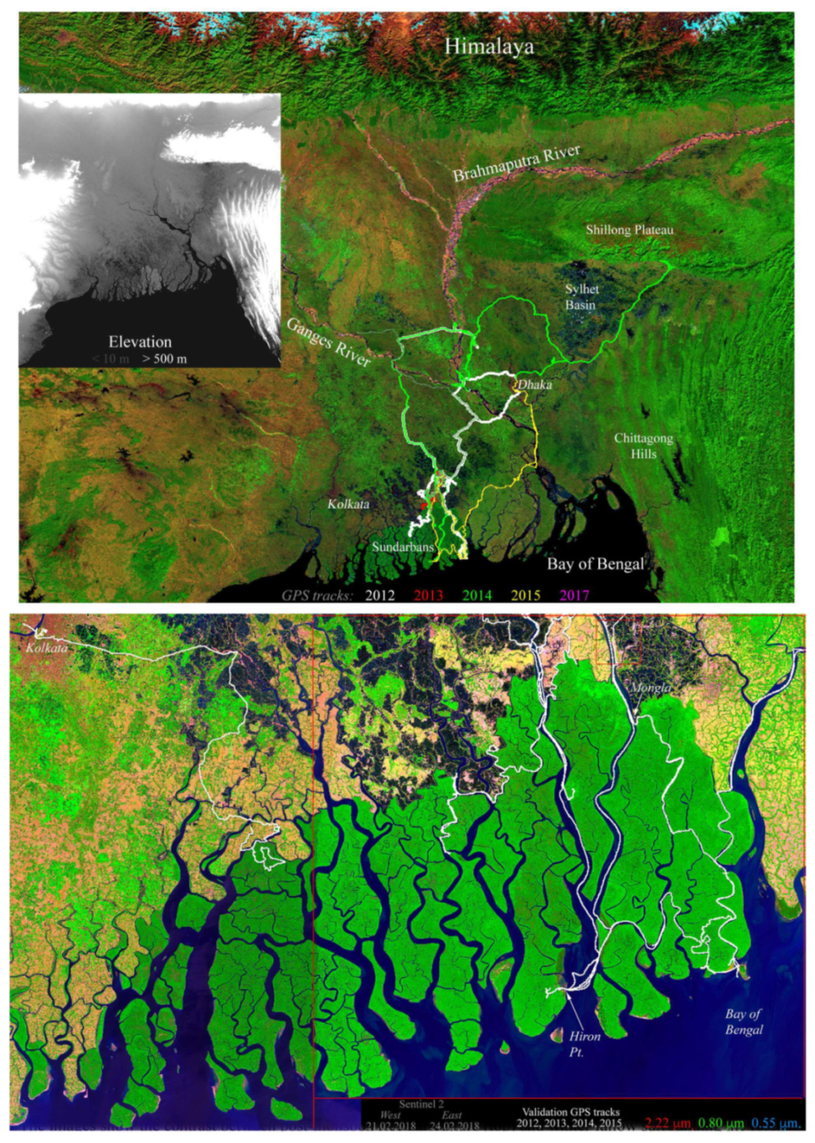
The Sundarban of the lower Ganges-Brahmaputra delta forms the largest contiguous mangrove forest on Earth. The ~10,000 km2 forest, along with its interlaced tidal channel systems, occupies much of the seaward extent of the Ganges-Brahmaputra delta (Figure 1) and provides habitat for an estimated 350 species of vascular plants, 300 species of birds, 250 species of fish, 42 species of mammals, 35 species of reptiles, and 8 species of amphibians. Charismatic megafauna dwelling in the Sundarban include the Gangetic dolphin, Saltwater crocodile, Monitor lizard, King cobra, Pangolin, Pteropus, Junglefowl, Chital deer, Rhesus macaque, Jungle cat, Indian leopard and the Bengal tiger. The floristic diversity of the Sundarban is also extraordinary, containing an estimated 40% of all mangrove species known worldwide. Charismatic megaflora of the Sundarban include Sundri (Heritiera fomes), Gewa (Excoecaria agallocha), Goran (Ceriops decandra), Keora (Sonneratia apetala), and Golpata (Nypa fruticans). The unusual floristic diversity of the Sundarban is partly a result of a longitudinal salinity gradient extending westward from the main channel of the Meghna River, which is the world’s third largest with an annual discharge of > 930 × 109 m3 of water. In addition, the annual sediment load of 1.9 × 10⁹ tons, the world’s largest, provides the silt and clay tidal flats upon which the mangroves have colonized. The protected Sundarban forest is surrounded to the west, north and east by densely populated agricultural communities in both Bangladesh and India. The balance between sediment deposition and erosion, in the context of sea level fluctuations, subsidence and river discharge, determines the evolution of the channel network within the mangroves and surrounding polders. Shoreline and riverbank changes in the mangrove reflect the net result of these processes. On decadal time scales, these changes have clear implications for both the mangroves and the ecosystems they support, as well as the communities living on the surrounding polders. For reasons of data availability (given below), the focus of this study is limited to the Bangladesh Sundarban, which comprises the eastern 60% of the forest.
3. Materials and Methods
This study is rooted in the spatiotemporal analysis framework of Empirical Orthogonal Function (EOF) characterization and Temporal Mixture Modeling (TMM) proposed by Reference [1]. This approach begins with EOF characterization based on the Principal Component (PC) transform. The PC transform computes the covariance (or correlation) matrix of the image time series and factors it into its corresponding eigenvalue and eigenvector pairs. Eigenvectors represent the dominant uncorrelated modes of spatiotemporal variability in the dataset, and their associated eigenvalues quantify the fraction of variance associated with each mode. The transformed time series are then examined in the optimized space of their low-order PCs, referred to as the Temporal Feature Space (TFS). In this space, the most statistically extreme time series occupy apexes of the data cluster. These extreme time series are referred to as temporal endmembers (tEMs). Edges connecting apexes correspond to binary mixtures, and pixels on the interior of the point cloud correspond to more complex mixtures of 3 or more tEMs. In the modeling phase, the tEMs are used as the basis vectors for a linear mixture model which represents every pixel time series as a linear combination of the tEMs (plus error). By representing the full space of temporal phenologies as combinations of the most statistically distinct tEMs, the model eliminates the need to make assumptions about the phenologies present in the data. Inversion of the linear mixture model then results in a set of continuous maps which show spatial patterns in the contribution of each tEM to the image time series. The temporal mixture model, and the corresponding temporal feature space on which it is based, are directly analogous to the spectral mixture modeling approach developed by References [2,3,4].
In this study we extend the Empirical Orthogonal Function (EOF) characterization and Temporal Mixture Modeling (TMM) approach to include two novel improvements, in order to reduce the impact of cloud contamination and phenological heterogeneity. Both may be incorporated prior to the Principal Component (PC) transformation that generates the spatial PCs and the temporal EOFs upon which the characterization is based. The first optional step is the application of a 3D cloud mask to the input spatiotemporal cube of vegetation fraction maps. The second optional step is the application of a Robust Principal Component Analysis (RPCA) to separate a low rank component time series dominated by phenology from a sparse component time series containing more transient features like cloud shadow.
The input data consist of a time series of coregistered 2D maps of vegetation abundance. In this analysis we use the newly developed Harmonized Landsat Sentinel-2 (HLS) S30 product provided by NASA (via hls.gsfc.nasa.gov), in addition to the archival Landsat Collection 1 Level 1 product provided by the USGS (via earthexplorer.usgs.gov). The HLS product combines imagery from the Landsat 8 Operational Land Imager (OLI) with imagery from the Sentinel-2 Multispectral Instrument (MSI) to produce time series of BRDF and atmospherically corrected reflectance products from 2015 until present [5]. We use the HLS S30 product (11 Sentinel-2 bands resampled to 30 m resolution) for the benefit of the additional NIR bands but limit the HLS analysis to 2018 because temporal coverage is much sparser for 2015–2017 (Table A1). Of the 88 acquisitions available for tile 45QYE, we begin with the 67 that are not completely cloud contaminated. Of these 67, 34 cover nearly the full tile extent while the remainder are sidelap acquisitions, covering less than half the tile on the western side. Of the 34 near-full tiles, 25 are mostly or completely cloud-free and the rest contain popcorn cumulus covering approximately 1/3 to 2/3 of the tile. Tile 45QYE covers all of the Bangladesh Sundarban, a small part of the Indian Sundarban and the densely populated polders (embanked islands) north and east of the Sundarban. The land cover on these polders consists of a complex mosaic of rice-dominant agriculture, shrimp-dominant aquaculture and forested embankments and levees where the inhabitants live. For a complementary analysis of decadal changes we use 22 mostly or completely cloud-free, post-monsoon (late October to early December), Landsat 5/7/8 acquisitions between 1989 and 2017 to characterize response to disturbances from cyclones, erosion, deposition and anthropogenic impacts.
3.1. Spectral Characterization of the HLS Time Series
Subpixel vegetation fractions are estimated for all products by inversion of a linear spectral mixture model using standardized spectral endmembers. Linear spectral unmixing provides accurate, scaleable estimates of rock and soil Substrate (S), illuminated photosynthetic Vegetation (V) and non-illuminated/absorptive Dark (D) targets like shadow and water. The simple 3 endmember SVD mixture model provides physically-based estimates of the three most spectrally and functionally distinct types of land cover, and has been shown to scale linearly from the 500 m resolution of MODIS [6] down to the 2 m resolution of WorldView-2 [7]. Standardized SVD endmembers are given for Landsats 4−8 by [8] and for Sentinel-2 by a global analysis of > 1.4 × 10⁸ spectra collected from spectral diversity hotspots worldwide. RMS misfits for pixel spectra unmixed with these standardized endmembers are < 0.05 for >94% of each global compilation of more than one hundred million spectra.
In addition to providing a general, and easily obtained, metric for the suitability of the SVD spectral mixture model, the RMS misfit can be used as the basis for a cloud mask. Because the SVD model does not include an endmember for clouds, pixel spectra affected by cloud often lie off the triangular plane of the model and can therefore have conspicuously larger RMS misfits than mixed spectra containing only land cover. As a result, RMS misfit distributions are strongly bimodal for most imagery containing clouds. By using the bivariate distribution of vegetation fraction and RMS misfit, it is straightforward to impose a simple linear decision boundary to distinguish cloudy pixel spectra with higher misfit from clear sky spectra with much lower misfit. While this approach can be generalized to incorporate more complex decision boundaries, or even multiple decision boundaries to provide a sensitivity analysis, we limit our attention to the case of a single linear decision boundary in this study. The decision boundary applied to the vegetation fraction and RMS misfit maps as a linear inequality yields a separate cloud mask for each image. When the time series of cloud masks is applied to the time series of vegetation maps, clouds are masked in 3D. Because this method allows partial cloud acquisitions to contribute information on dates when clear sky images are not available, substantially more data are made available for the EOF analysis than would be possible with more standard approaches of either (1) entirely eliminating partially cloud-contaminated scenes, or (2) entirely eliminating partially cloud-contaminated pixel time series.
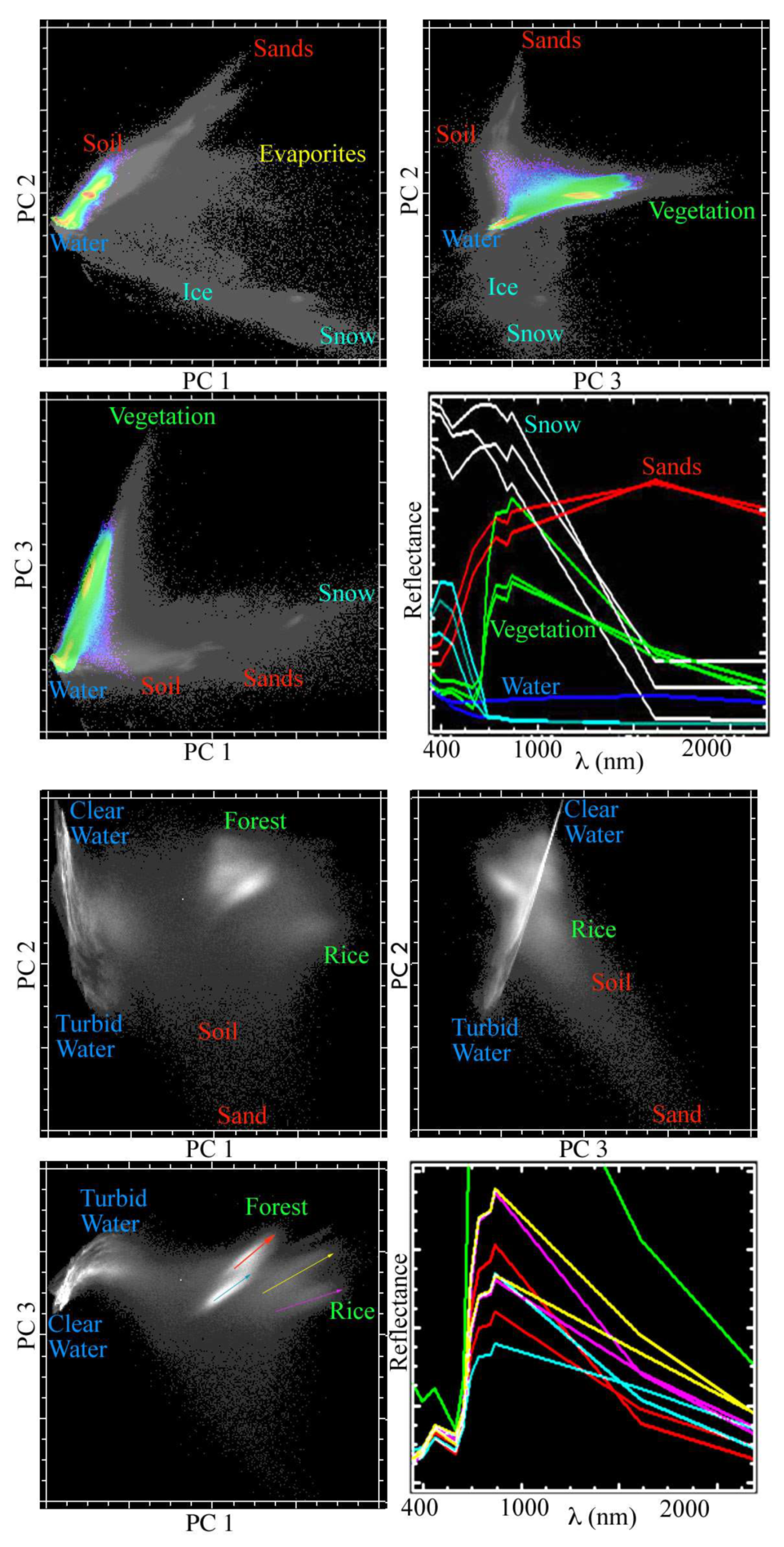
Before using the standardized spectral mixture model to estimate per pixel vegetation abundance, we verify that the local spectral mixing space of the Sundarban HLS tile lies within the global mixing space bounded by the standardized endmembers. The spectral feature space of a single cloud-free post-monsoon Sentinel-2 acquisition from the eastern Sundarban HLS tile is shown in Figure 2. The upper 3 scatterplots show the diversity of pixel reflectances from the 3 low order Principal Components of the tile projected onto a silhouette of the feature space of the 140 million Sentinel-2 spectra used to define the global space and identify the bounding spectral endmembers. These bounding endmembers, with both internal and external bounds, are shown in the plot in the lower right of the top panel. The density shaded distributions of the single tile (in color) are seen to occupy a relatively small part of the full global feature space, yet the Sundarban space clearly distinguishes at least 4 distinct spectral mixing trends corresponding to different vegetation reflectances mixing with canopy shadow. As expected, the Sundarban tile is dominated by binary mixtures of water/shadow and vegetation, with little exposed dry substrate and no snow, ice or evaporates.
The lower 3 scatterplots show orthogonal projections of the single date Sentinel-2 bands rotated on the basis of their own covariance matrix. Freed of the constraint of the global feature space, this projection reveals the internal structure of the nearly binary mixing continuum from the global space above. In addition to a continuum of clear to turbid river water, the local Sentinel-2 space resolves two distinct mixing continua for forests and two more diffuse mixing continua for the extensive areas of rice cultivation that are pervasive throughout the delta following the summer monsoon. Example spectra are given for the low amplitude dark (shaded) and high amplitude bright (illuminated) endmembers of each continuum. While these endmembers could be used as the basis for a more complex mixture model, we use the global SVD endmembers to derive estimates of generic vegetation fraction for the spatiotemporal analysis in order to condense the information content into a time series of a single, consistent variable. For comparison, a Visible + Near IR + SWIR (VNS) reflectance composite is combined with a SVD endmember fraction composite in Figure 3.
3.2. Spatiotemporal Characterization of the Vegetation Fraction Time Series
Robust Principal Component Analysis (RPCA, [9]) considers an image time series M to be the sum of a low-rank matrix L and a sparse matrix S:
L contains features which vary gradually (e.g., forest phenology) or are invariant (e.g., static stretches of coastline), and S contains short-lived and spatially limited features (e.g., clouds, agriculture). The matrix decomposition is generally ill-posed (NP-hard), but under weak assumptions [9] proves that L and S can be recovered exactly through a convex optimization program called Principal Component Pursuit. This works by optimizing the sum of the nuclear norm of L (L*; sum of the singular values) and the weighted L1 norm of S:
where L is a rectangular matrix of dimensions n1 × n2 and
An important benefit of the RPCA approach is that no tuning parameters are required.
RPCA has been applied to a wide range of image analysis problems in recent years, including image restoration, hyperspectral image denoising, face recognition, multifocus imaging, change detection, medical imaging, imaging for 3-D computer vision, and video processing. Despite the recent attention focused on RPCA, however, to our knowledge the method has not yet been applied for the purposes of multitemporal satellite image analysis or phenological characterization.
In this analysis, we implement RPCA using the Alternating Direction Method of Reference [10] as implemented in the R package “rpca” [11]. We use the values of λ and µ (augmented Lagrange multiplier parameter) suggested by Reference [9]. The terminal δ was set to 1 × 10⁻⁷, which reached convergence within 5000 iterations in every case, and often within 2000 iterations, for image time series a spatial extent of > 1 × 106 pixels and > 20 temporal dimensions. This corresponded to ≈ 4–6 hour processing times using a dual-core 2.6 GHz CPU with 24 GB of RAM.
4. Results
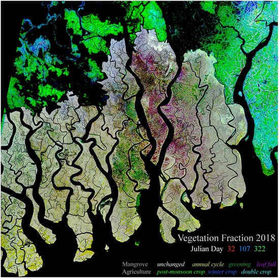
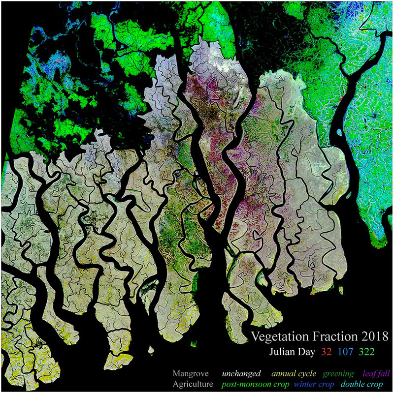
Once the vegetation fraction maps have been estimated for each HLS tile date, the vegetation fraction map time series is constructed for exploratory data analysis before the spatiotemporal analysis is done. Spatiotemporal variability of the HLS-derived vegetation fraction time series is illustrated in Figure 4. A tri-temporal composite of vegetation maps from pre-monsoon early summer, post-monsoon autumn and dry season winter reveals spatially coherent differences in vegetation phenology. Because the vegetation maps are derived using the same spectral endmembers and are stretched identically, color implies change in the tri-temporal composite. If the mangrove vegetation were literally evergreen, as is often assumed, the mangroves would appear as shades of gray. The lower part of Figure 4 shows a full resolution 10 × 10 km subset as a time-space cube. The front face of the cube shows the tri-temporal composite, with a Gaussian stretch applied to the vegetation fraction distributions of the 3 dates, while the sides show the temporal evolution of the pixel time series along the top and right edges of the cube. The post-monsoon greening is apparent following the band of gaps (black) associated with monsoon cloud cover that has been masked. Cloud shadows cannot be reliably distinguished from lower vegetation fractions associated with canopy structure and water, so they are not masked and remain on cloudy dates throughout the cube. The coherent internal structure of the full resolution tri-temporal map suggests potentially physically meaningful variations in vegetation abundance or canopy closure at the decameter to hectometer scale. While this structure may be partly dependent on species composition, it is not necessarily resolvable spectrally in a single image. The tri-temporal image clearly maps phenological phase differences, albeit on only three dates. The spatiotemporal analysis identifies such phase differences on the basis of the entire cube of vegetation abundance.
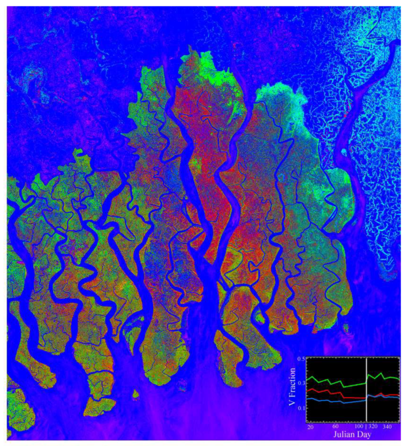
The combination of mangrove forest, forested levees and the extensive diversity of single and multi-crop agriculture poses a challenge for spatiotemporal analysis of mangrove phenology because the spatiotemporal variability of the agricultural phenology contributes more to the covariance structure than does the mangrove phenology. Figure 5 shows the result of a standard PC transform on the masked HLS time series of full tile coverages. The color composite of spatial PCs 1, 2, and 3 is spatially coherent, yet distressingly colorful. The wide range of colors implies a wide range of phenologies represented by a wide range of linear combinations of the three low order components. This complexity is borne out by the inset temporal feature space in Figure 5. While fully 3D, the structure of the temporal feature space is dominated by the continuum of agricultural phenologies composed of extensive post-monsoon rice and a variety of irrigated winter crops. Any variability in the phenology of the mangroves is compressed into the forest cluster. This compression is also indicated by the relatively homogeneous green of the mangroves. Unlike reflectance images, the PC composites reveal temporal rather than spectral patterns. The band combination was deliberately chosen to make the mangrove forest appear green and the water blue to maintain colorific equipoise.
Applying the RPCA to separate the low rank (L) and sparse (S) components of the time series very effectively distinguishes the transient phenological diversity of the agriculture from the more consistent phenology of the mangrove forest. Figure 6 shows low order PC composites for the PC transform of each of the L and S component time series. Although the composite maps in Figure 6 are analogous to that in Figure 5, the results are strikingly different. The low rank component shows the agricultural fields are a relatively homogenous blue with aquaculture ponds in magenta (separated by forested levees in green) while revealing a spatially coherent continuum of reds, browns and greens within the mangrove forest. Notice the similarity of the structure of the PC composite of the Low Rank component and the tri-temporal composite in Figure 4. The important distinction is that the PC composite in Figure 6 is based on the full image time series, not just three time steps. Notice also the difference between the Low Rank temporal feature space in Figure 6 and the standard PC temporal feature space in Figure 5. The former expands the structure of the feature space to reveal two distinct forest clusters separating the forested embankments and levees from the areas deeper within the mangrove. The 2D forest cluster of the standard PCA has now been expanded to a quasi-triangular main cluster and a more elliptical cluster beneath it. This suggests that the mangrove forest may have additional phenological diversity that is not represented in a straightforward way by the standard PCA. In contrast, the PC composite of the Sparse Component reveals the true complexity of the agricultural areas, as well as residual cloud contamination within the mangrove that has been separated from the Low Rank component.
The RPCA separation of agricultural from mangrove phenology effectively expands the structure of the forest cluster in the temporal feature space, making it possible to identify three apexes bounding all the forest pixels in the PC1/PC2 projection. Temporal EMs are identified from each apex and used as the basis for a simple ternary temporal mixture model of the forest (Figure 7). The tEMs differ in both greenness (overall amplitude) and seasonality (annual range) with the green and blue tEMs showing the greatest post-monsoon increase in greenness and the red tEM showing an overall decrease without post-monsoon greening. The resulting fraction map (Figure 7) shows large, spatially contiguous areas dominated by each tEM (red, green, blue), but more of the map corresponds to mixtures (orange and cyan). Because the river channels, aquaculture and agriculture areas lie outside the triangular model and adjacent to the low amplitude blue tEM, their fraction estimates project onto the model near that tEM and appear blue and magenta. The alternating increase and decrease in the vegetation fraction of the tEMs is believed to result from imperfect correction of the BRDF (Claverie and Ju, Pers. Comm.).
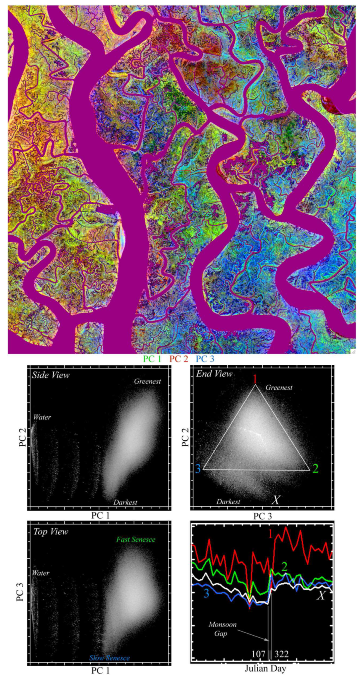
The RPCA results for the full tile partial/cloud free images suggest that the approach might be effective on the smaller, denser time series within the sidelap on the western edge of the tile. The benefit of using a denser but noisier time series is twofold. It allows us to test the robustness of the RPCA while better characterizing the variance on shorter period revisits. Figure 8 shows the result of applying the same RPCA approach to the 10 × 10 km substack of the mangrove forest shown previously in Figure 4. Again, the PC composite of the Low Rank component shows spatially coherent structure that is similar in form to the phenological phase shifts seen in the tri-temporal composite in Figure 4. However, as above, the PC composite is based on the full time series of vegetation maps, after the more transient Sparse component has been removed. The temporal feature space of the Low Rank component shows a sub-triangular to diamond-shaped cluster for the forest areas. We identify 4 temporal endmembers (tEMs) from the apexes of this cluster and use them as the basis for a temporal mixture model (Figure 9). The higher vegetation fraction tEM in red maintains higher fractions throughout the year but with more variability. The three lower fraction tEMs show different rates of post-monsoon senescence, revealing the source of the phenologic variability. However, the tEM labeled X appears to be a nearly linear combination of the faster and slower senescing tEMs. When all 4 tEMs are used in the temporal mixture model, the result shows considerable overfitting as negative fractions, suggesting that the similarity of the tEMs has destabilized the inversion. When the X tEM is removed from the model, the resulting 3 tEM model inversion gives feasible fractions in the 0 to 1 range. The result of this inversion is shown in Figure 9.
4.1. Vicarious Phenological Validation
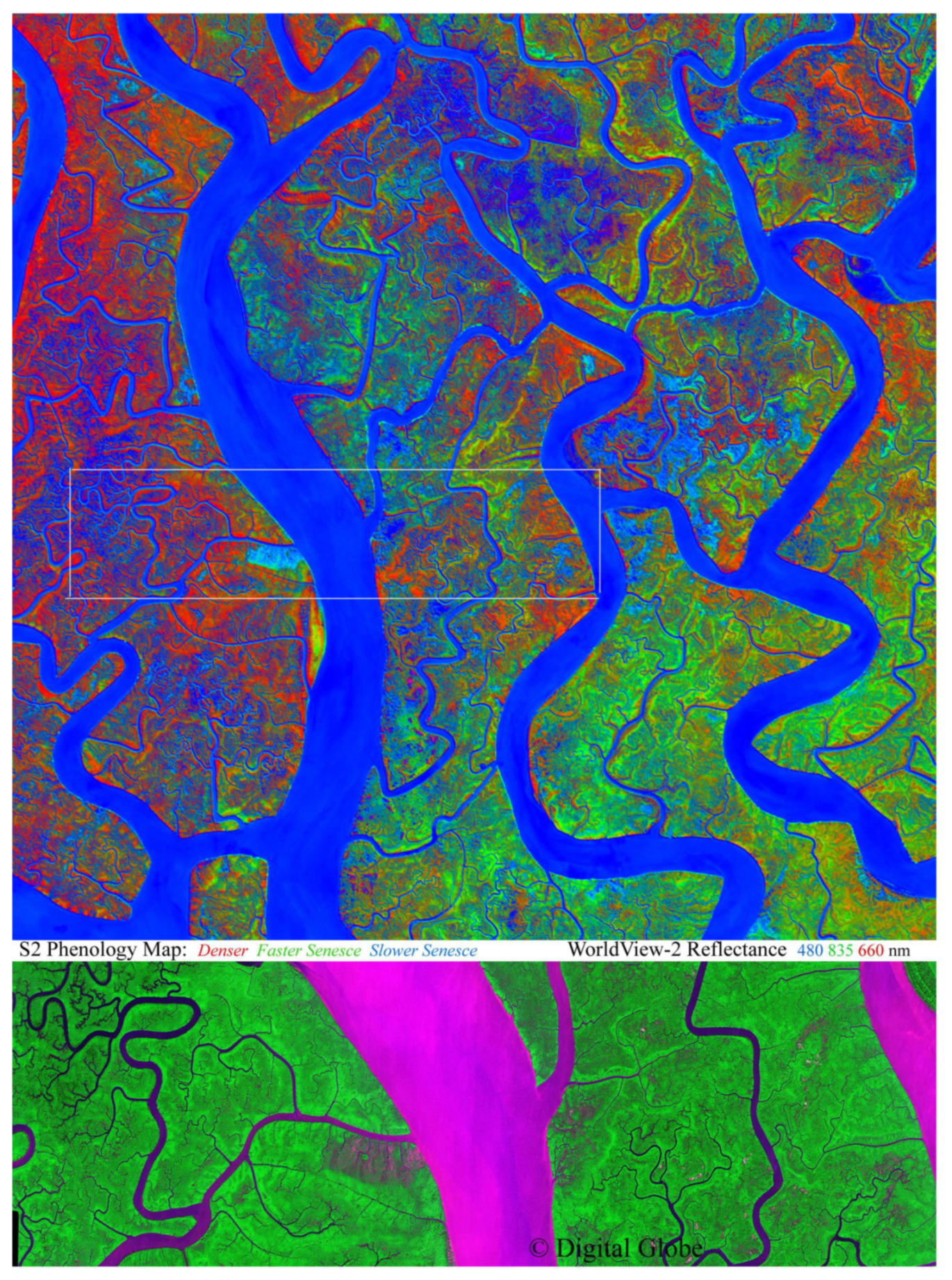
As with the PC composite, the phenological fraction map is spatially coherent. When compared with a 2 m WorldView-2 image (Figure 9), a clear correspondence is seen between the density of canopy closure (greenness) in the WV2 image and in the relative prominence of the corresponding tEM fractions in the phenology map. While this qualitative comparison does not provide true validation, it does suggest that the spatial correspondence between canopy closure (hence shadow fraction) at 2 m resolution and phenology at 30 m may be due, in part, to variations in species composition.
4.2. Interannual Change
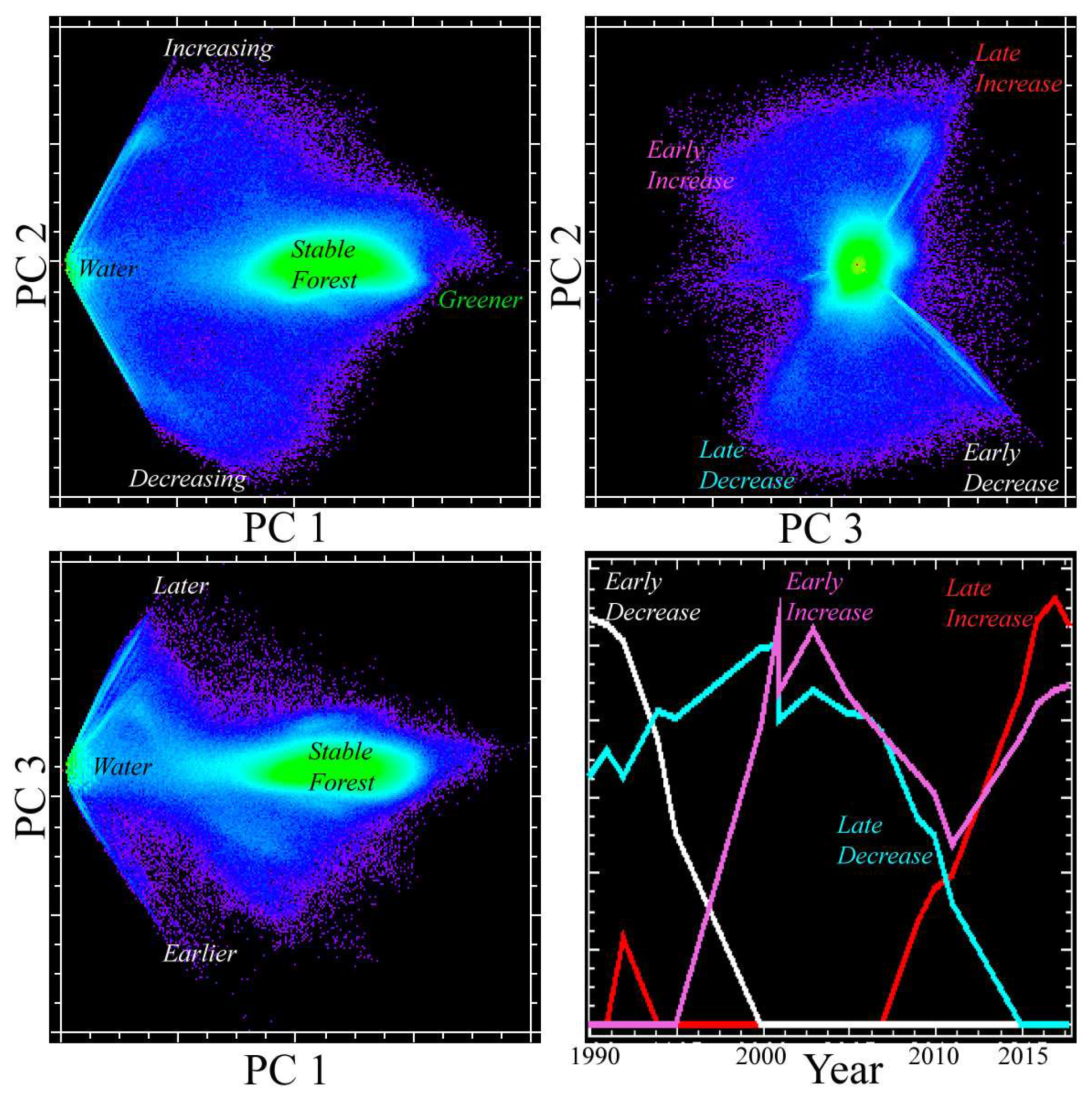
Having established the presence, and biophysical plausibility, of local scale variability within the Sundarban mangrove forest, we now extend the analysis to interannual variability and disturbance response. For analysis of interannual changes and disturbance response, we use the time series of near-anniversary post-monsoon Landsat images from late October to early December 1989-2017. Specifically, we examine the substack from the SE section of the Sundarban that can be inscribed in a rectangle containing no agriculture. Because nearly/cloud-free images are available in this time window, we begin with a standard EOF analysis without the use of RPCA, using only mixture model misfit masking on the few partial cloud acquisitions. A standard PC transform of the 20 date time series of the Landsat subscene produces the temporal feature space shown in Figure 10. The ellipsoidal cluster representing forest shows no internal structure but an axis aligned with water representing the overall level of tree canopy density given by the vegetation fraction. The important changes are in the four mixing lines bounding the two binary mixing planes extending outward from the water (i.e., constant low) vegetation fraction. These two planes represent varying combinations of late and early increasing and decreasing vegetation abundance. These continua correspond to the expansions and contractions of the forest associated with shoreline advance and retreat. Example time series of vegetation abundance from the apexes of the PC 3/2 “bowtie” are shown in the accompanying tEM plot.
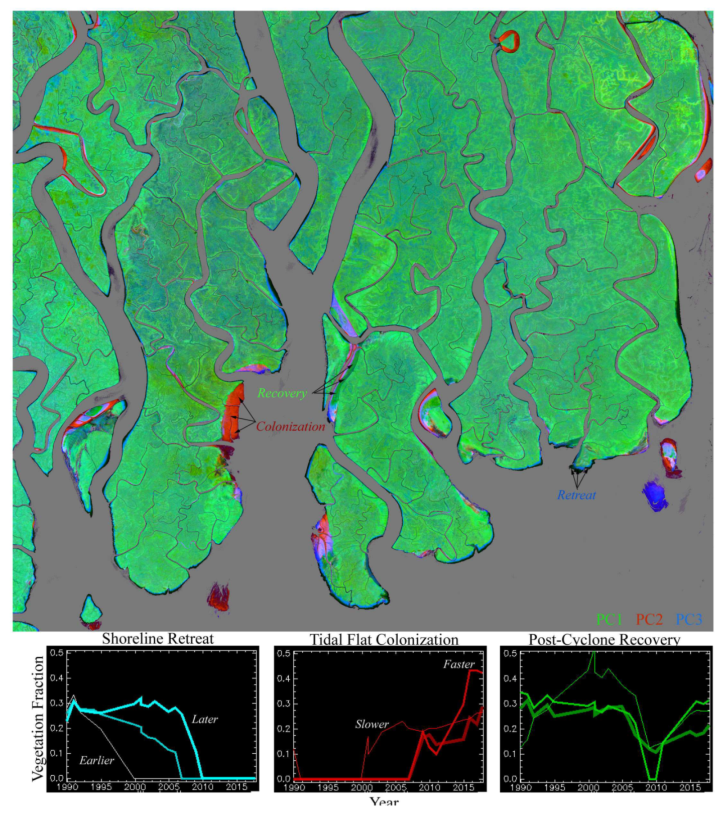
The spatial PCs resulting from the EOF analysis of the post-monsoon anniversary vegetation maps are sufficiently distinct to serve as a disturbance map. Figure 11 shows a low order PC composite for the SE section of the Sundarban used to produce the temporal feature space shown in Figure 10. Because the mean has not been removed, PC1 shows the temporal mean vegetation abundance in green. PC maps 2 and 3 are shown in red and blue. They correspond to decadal increases and decreases in vegetation abundance corresponding to disturbances.
It is clear from the map in Figure 11 that the dominant disturbances in this area are almost all related to shoreline and riverbank advances and retreats. The changes are dominated by elongate thin bands of retreating shoreline (blue and black) and broader, more localized, patches of vegetation-colonized mudflats (red and pink). Most of these disturbances show progressions parallel to the direction of advance or retreat. Examples of the progression of vegetation loss or gain are given by the temporal trajectories of individual pixels shown below the PC map. The trajectories span the full range between gradual, nearly linear, progressions to abrupt changes. A more detailed analysis of these changes is given by Reference [12].
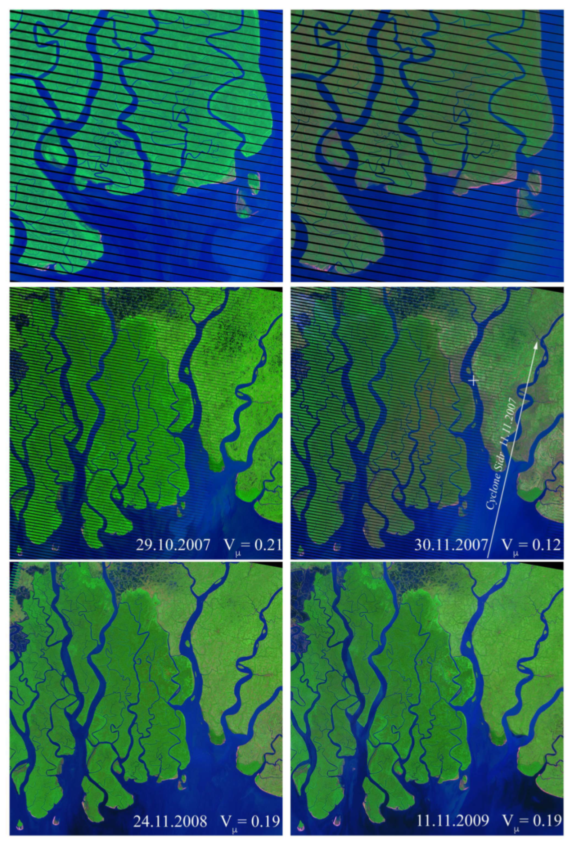
The EOF analysis of the post-monsoon Landsat images shows no overall trend in vegetation abundance of the Bangladesh Sundarban between 1989 and 2017 – specifically, the temporal EOF corresponding to the 1st (green) spatial PC shown in Figure 11 shows no obvious trend. However, there have been cyclones during this time interval that may have created disturbances that might appear in EOF 1. The cyclone with the highest wind speed, Cyclone Sidr in 2007, occurs in a year with no cloud-free Landsat 5 acquisitions post-monsoon. Fortunately, Landsat 7 did acquire cloud-free images within a month before and after Cyclone Sidr. Because of the Scan Line Corrector gap problem with Landsat 7, we cannot incorporate these images into the spatiotemporal analysis. However, they do provide qualitative information relevant to the question of disturbance recovery. Figure 12 shows a succession of Landsat images before and after Cyclone Sidr passed to the immediate east of the Sundarban. The false color composites, using identical stretches, show a clear defoliation event between 29 October 2007 and 30 November 2007 with extensive areas changing from green to brown as the NIR reflectance drops relative to the SWIR and visible reflectance. This is consistent with the defoliation that would be expected given Sidr’s 140 km/hr wind speed estimates. However, subsequent post-monsoon Landsat images from 2008 and 2009 suggest that the mangrove’s vegetation fraction distribution had recovered within one year (Figure 12).
5. Discussion
The principal finding of the 2018 phenological mapping is the presence of at least three distinct phenologies, two of which are punctuated by the monsoon, while the third may reflect a longer period interannual process. The complex spatial patterns of these phenologies span a wide range of spatial scales but are spatially contiguous, suggesting a biophysical origin. These spatial patterns are both concordant and discordant with mapped species distributions, suggesting the influence of environmental processes as well as species response. The complexity of the phenology map is consistent with the floristic diversity of the Sundarban [13] and the complexity of its surface hydrology.
The most current understanding of tree species distribution for the Bangladesh Sundarban is based, in part, on surveys conducted by the Bangladesh Forest Department in 2014 [14]. Stratified, non-random sampling was conducted along transect lines in 190 “streamside” and 130 “forest proper” settings. Species richness was quantified using both Simpson’s and Shannon’s diversity indices. The ANOVA and PCA of the 320 transects allowed the authors to coanalyze traits such as species abundance, species richness, species diversity, and family dominance. However, the coverage is not sufficient to provide a full coverage species composition map. The species composition map shown in Figure 1 of Reference [14] is similar to the 2017 map published by the Bangladesh Forest Department (although with a different class/color scheme), but no details are provided about the production of either. Both of these maps are qualitatively similar, although significantly less detailed, than the 2002 map, which contains a brief explanation of sources. The 2002 map is based on visual interpretation of a 1:50,000 SPOT image from 1989 in combination with 1:15,000 airphotos from 1995. Accuracy estimates are not provided, although the 2002 map does acknowledge checking.
Qualitative comparison of the Bangladesh Forest Department species composition maps with the HLS-derived phenology map show several conspicuous examples of coincident species and phenology boundaries - as well as several disparate examples of boundaries and gradients in each not coinciding with the other. In other words, the species composition and phenology maps neither agree nor disagree consistently enough to support or refute a causative relationship between the two. As a result, the most conservative interpretation is that many mapped species transitions do correspond to observed phenology transitions, but many others do not. And many phenology transitions have no obvious correspondence to mapped species transitions. However, both maps contain spatially contiguous patterns spanning a range of scales, suggesting biophysical origins for the patterns. The overall regional gradations in tEM dominance in the R, G, B phenology fraction map (Figure 7) generally correspond to the gradations among Sundri, Goran, and Gewa species dominance (respectively) seen on the species composition map. Together, the simultaneous agreement and disagreement of the two maps suggest that other factors may influence phenology within and across species distributions. Given the conspicuous increase in vegetation abundance after the monsoon, following annual decreases, it seems logical to expect dry season surface hydrology to affect phenology – perhaps at least as strongly as species composition. All of which emphasizes the importance of interannual analyses of the HLS time series as more years become available. While the distinct phenologies and their spatial patterns are compelling, it remains to be seen how consistent these patterns are from year to year. Their persistence, or transience, may itself inform our understanding of the ecology of the largest, most biodiverse mangrove forest on Earth.
The RPCA proposed by Reference [9] appears to be effective for separating spatially localized transients like sparse cloud cover and variations in agricultural phenology from the more subtle, longer period changes in mangrove forest greenness related to leaf fall. This is consistent with the observations of Pastor Guzman et al. [15] who demonstrated annual cycles in mangrove greenness on the coast of the Yucatan Peninsula in Mexico using MODIS imagery. In addition to regional scale patterns similar to those observed by Pastor-Guzman and colleagues, we also observe finer scale spatially coherent phase shifts in the greening-senescence cycle in the Bangladesh Sundarban. These finer scale variations are presumably a result of both species composition and local environmental factors. Prior to the study of Rahman and Islam [16] in 2015, only two studies of Sundarban phenology had been published, and both focused on seed and fruit production. Rahman and Islam [16] investigated phenophases of the 5 most common mangrove species in the Sundarban (Sundri, Kankra, Gewa, Goran, and Passur) between 2005 and 2014 across three salinity zones. They found two overlapping phases of leaf appearance and shedding times (prior to monsoon), with no variation with respect to salinity – in contrast to flowering, fruiting and seed dropping, which showed some variation with salinity. However, the labor intensive nature of individual tree monitoring limited the study to five trees per species and was not intended to provide species composition maps beyond the individual trees observed.
The phenologies revealed by the HLS characterization also suggest that longer period interannual processes may contribute to spatiotemporal variance in the Sundarban mangrove forest. For longer baseline interannual observations it is possible to reduce both cloud contamination and data processing through the use of dry season anniversary images when the dry season coincides with river discharge minima. Nonetheless, tidal phase must be considered when interpreting changes that may be due to shallow tidal flats that may expose or conceal large areas within river channels. On decadal time scales the changes in forested shoreline and riverbank locations within the Sundarban are sufficient to show progressive patterns of shoreline advance and retreat simultaneously - regardless of tidal phase. In part, this is due to the presence of cut banks, which can erode quickly, causing mass slumping of mature forest into river channels [12]. While the most conspicuous interannual changes are related to multi-year shoreline erosion and deposition, cyclone-driven defoliation and recovery are also detected. In the most severe case of Cyclone Sidr in 2007, very little erosion was observed and the defoliated areas had fully recovered within a year, suggesting that the mangroves are well-adapted to the frequent cyclones of the Bay of Bengal.
6. Conclusions
The RPCA of the HLS time series clearly separates the effects of multi-crop agriculture and intermittent cloud and cloud shadow from the longer period cycle of mangrove senescence and greening. In doing so, it enables a standard EOF analysis of the Low Rank component to identify distinct phenological modes within the mangrove forest. These modes are manifest as spatially coherent patterns of delayed greening relative to the monsoon. These phenological phase shifts occur at scales ranging from 100 to 10,000 meters. The fact that these phenology patterns are spatially coherent but both concordant and discordant with species composition maps suggests that the phenology is influenced both by species composition and environmental factors like surface hydrology. Decadal changes related to shoreline erosion and deposition and canopy closure can be identified with a standard EOF analysis if sufficient cloud-free images are available. EOF analysis of post-monsoon Landsat imagery clearly identifies disturbance related to erosion and deposition of the mud/silt substrate on which the forest depends. In the 1989–2017 period of this study, only Cyclone Sidr (11 November 2007) produced a measureable, but not spatially uniform, defoliation of the Sundarban tree canopy. However, this defoliation was undetectable one year later after the 2008 monsoon allowed regrowth. This suggests that the impact of cyclones on the mangrove canopy may be limited in time and extent by species composition and canopy roughness.
Author Contributions
Conceptualization, C.S. and D.S.; methodology, C.S. and D.S.; formal analysis, C.S. and D.S.; data curation, C.S.; writing—original draft preparation, C.S.; writing—review and editing, C.S. and D.S.; visualization C.S.; funding acquisition, C.S. and D.S.
Funding
Work done by D. Sousa was conducted with Government support under FA9550-11-C-0028 and awarded by the Department of Defense, Air Force Office of Scientific Research, National Defense Science and Engineering Graduate (NDSEG) Fellowship, 32 CFR 168a. CS was supported by the NASA MultiSensor Land Imaging program (grant NNX15AT65G) and the Office of Naval Research (grant N000-14-11-1-0653).
Acknowledgments
We thank Manu Lall for suggesting alternative PCA approaches that led to exploration of RPCA. We acknowledge the USGS for providing Landsat imagery and NASA for providing the HLS products. M. Claverie and J. Ju provided informative details on the production of the HLS product.
Conflicts of Interest
The authors declare no conflict of interest.
Appendix A

Table A1.
HLS Sentinel-2 scenes.
| HLS Tile ID | JD | FY | C | HLS Tile ID | JD | FY | C |
|---|---|---|---|---|---|---|---|
| HLS.S30.T45QYE.2018002 | 2 | 2018.005 | p | HLS.S30.T45QYE.2018192 | 192 | 2018.526 | p |
| HLS.S30.T45QYE.2018005 | 5 | 2018.014 | c | HLS.S30.T45QYE.2018195 | 195 | 2018.534 | p |
| HLS.S30.T45QYE.2018010 | 10 | 2018.027 | c | HLS.S30.T45QYE.2018200 | 200 | 2018.548 | p |
| HLS.S30.T45QYE.2018012 | 12 | 2018.033 | c | HLS.S30.T45QYE.2018220 | 220 | 2018.603 | p |
| HLS.S30.T45QYE.2018015 | 15 | 2018.041 | c | HLS.S30.T45QYE.2018222 | 222 | 2018.608 | p |
| HLS.S30.T45QYE.2018017 | 17 | 2018.047 | c | HLS.S30.T45QYE.2018227 | 227 | 2018.622 | p |
| HLS.S30.T45QYE.2018022 | 22 | 2018.06 | c | HLS.S30.T45QYE.2018230 | 230 | 2018.63 | p |
| HLS.S30.T45QYE.2018025 | 25 | 2018.068 | c | HLS.S30.T45QYE.2018237 | 237 | 2018.649 | p |
| HLS.S30.T45QYE.2018030 | 30 | 2018.082 | c | HLS.S30.T45QYE.2018240 | 240 | 2018.658 | p |
| HLS.S30.T45QYE.2018032 | 32 | 2018.088 | c | HLS.S30.T45QYE.2018252 | 252 | 2018.69 | p |
| HLS.S30.T45QYE.2018035 | 35 | 2018.096 | c | HLS.S30.T45QYE.2018257 | 257 | 2018.704 | p |
| HLS.S30.T45QYE.2018037 | 37 | 2018.101 | p | HLS.S30.T45QYE.2018260 | 260 | 2018.712 | p |
| HLS.S30.T45QYE.2018040 | 40 | 2018.11 | c | HLS.S30.T45QYE.2018262 | 262 | 2018.718 | p |
| HLS.S30.T45QYE.2018045 | 45 | 2018.123 | p | HLS.S30.T45QYE.2018267 | 267 | 2018.732 | p |
| HLS.S30.T45QYE.2018047 | 47 | 2018.129 | c | HLS.S30.T45QYE.2018270 | 270 | 2018.74 | p |
| HLS.S30.T45QYE.2018050 | 50 | 2018.137 | p | HLS.S30.T45QYE.2018272 | 272 | 2018.745 | p |
| HLS.S30.T45QYE.2018052 | 52 | 2018.142 | c | HLS.S30.T45QYE.2018275 | 275 | 2018.753 | c |
| HLS.S30.T45QYE.2018055 | 55 | 2018.151 | c | HLS.S30.T45QYE.2018277 | 277 | 2018.759 | p |
| HLS.S30.T45QYE.2018060 | 60 | 2018.164 | c | HLS.S30.T45QYE.2018280 | 280 | 2018.767 | c |
| HLS.S30.T45QYE.2018065 | 65 | 2018.178 | p | HLS.S30.T45QYE.2018287 | 287 | 2018.786 | p |
| HLS.S30.T45QYE.2018067 | 67 | 2018.184 | c | HLS.S30.T45QYE.2018290 | 290 | 2018.795 | c |
| HLS.S30.T45QYE.2018070 | 70 | 2018.192 | c | HLS.S30.T45QYE.2018292 | 292 | 2018.8 | p |
| HLS.S30.T45QYE.2018072 | 72 | 2018.197 | p | HLS.S30.T45QYE.2018295 | 295 | 2018.808 | c |
| HLS.S30.T45QYE.2018082 | 82 | 2018.225 | p | HLS.S30.T45QYE.2018300 | 300 | 2018.822 | p |
| HLS.S30.T45QYE.2018085 | 85 | 2018.233 | p | HLS.S30.T45QYE.2018307 | 307 | 2018.841 | p |
| HLS.S30.T45QYE.2018087 | 87 | 2018.238 | p | HLS.S30.T45QYE.2018310 | 310 | 2018.849 | p |
| HLS.S30.T45QYE.2018097 | 97 | 2018.266 | p | HLS.S30.T45QYE.2018312 | 312 | 2018.855 | c |
| HLS.S30.T45QYE.2018100 | 100 | 2018.274 | p | HLS.S30.T45QYE.2018315 | 315 | 2018.863 | c |
| HLS.S30.T45QYE.2018102 | 102 | 2018.279 | p | HLS.S30.T45QYE.2018317 | 317 | 2018.868 | c |
| HLS.S30.T45QYE.2018105 | 105 | 2018.288 | p | HLS.S30.T45QYE.2018320 | 320 | 2018.877 | c |
| HLS.S30.T45QYE.2018107 | 107 | 2018.293 | c | HLS.S30.T45QYE.2018322 | 322 | 2018.882 | c |
| HLS.S30.T45QYE.2018122 | 122 | 2018.334 | p | HLS.S30.T45QYE.2018325 | 325 | 2018.89 | p |
| HLS.S30.T45QYE.2018132 | 132 | 2018.362 | p | HLS.S30.T45QYE.2018327 | 327 | 2018.896 | c |
| HLS.S30.T45QYE.2018135 | 135 | 2018.37 | p | HLS.S30.T45QYE.2018330 | 330 | 2018.904 | p |
| HLS.S30.T45QYE.2018137 | 137 | 2018.375 | p | HLS.S30.T45QYE.2018332 | 332 | 2018.91 | c |
| HLS.S30.T45QYE.2018147 | 147 | 2018.403 | p | HLS.S30.T45QYE.2018335 | 335 | 2018.918 | c |
| HLS.S30.T45QYE.2018152 | 152 | 2018.416 | p | HLS.S30.T45QYE.2018337 | 337 | 2018.923 | c |
| HLS.S30.T45QYE.2018155 | 155 | 2018.425 | p | HLS.S30.T45QYE.2018345 | 345 | 2018.945 | c |
| HLS.S30.T45QYE.2018157 | 157 | 2018.43 | p | HLS.S30.T45QYE.2018347 | 347 | 2018.951 | c |
| HLS.S30.T45QYE.2018160 | 160 | 2018.438 | p | HLS.S30.T45QYE.2018355 | 355 | 2018.973 | c |
| HLS.S30.T45QYE.2018165 | 165 | 2018.452 | p | HLS.S30.T45QYE.2018357 | 357 | 2018.978 | c |
| HLS.S30.T45QYE.2018167 | 167 | 2018.458 | p | HLS.S30.T45QYE.2018360 | 360 | 2018.986 | c |
| HLS.S30.T45QYE.2018170 | 170 | 2018.466 | p | HLS.S30.T45QYE.2018362 | 362 | 2018.992 | c |
| HLS.S30.T45QYE.2018187 | 187 | 2018.512 | p | HLS.S30.T45QYE.2018365 | 365 | 2019.000 | c |
Tile Coverage: Full Tile Partial Tile Cloud Cover: p = partial cloud c = clear sky.
References
- Small, C. Spatiotemporal dimensionality and Time-Space characterization of multitemporal imagery. Remote Sens. Environ. 2012, 124, 793–809. [Google Scholar] [CrossRef] [Green Version]
- Adams, J.B.; Smith, M.O.; Johnson, P.E. Spectral mixture modeling: A new analysis of rock and soil types at the Viking Lander 1 site. J. Geophys. Res. Solid Earth 1986, 91, 8098–8112. [Google Scholar] [CrossRef]
- Smith, M.O.; Johnson, P.E.; Adams, J.B. Quantitative determination of mineral types and abundances from reflectance spectra using principal components analysis. J. Geophys. Res. Solid Earth 1985, 90, C797–C804. [Google Scholar] [CrossRef]
- Gillespie, A. Interpretation of residual images: Spectral mixture analysis of AVIRIS images, Owens Valley, California. In Proceeding Second Airborne Visible/Infrared Imaging Spectrometer (AVIRIS) Workshop; NASA Jet Propulstion Lab: Pasadena, CA, USA, 1990; pp. 243–270. [Google Scholar]
- Claverie, M.; Ju, J.; Masek, J.G.; Dungan, J.L.; Vermote, E.F.; Roger, J.C.; Skakun, S.V.; Justice, C. The Harmonized Landsat and Sentinel-2 surface reflectance data set. Remote Sens. Environ. 2018, 219, 145–161. [Google Scholar] [CrossRef]
- Sousa, D.; Small, C. Globally Standardized MODIS Spectral Mixture Models. Remote Sens. Lett. 2019, 10, 1018–1027. [Google Scholar] [CrossRef]
- Small, C.; Milesi, C. Multi-scale standardized spectral mixture models. Remote Sens. Environ. 2013, 136, 442–454. [Google Scholar] [CrossRef] [Green Version]
- Sousa, D.; Small, C. Global cross-calibration of Landsat spectral mixture models. Remote Sens. Environ. 2017, 192, 139–149. [Google Scholar] [CrossRef] [Green Version]
- Candès, E.J.; Li, X.; Ma, Y.; Wright, J. Robust principal component analysis? J. ACM 2011, 58, 11. [Google Scholar] [CrossRef]
- Yuan, X.; Yang, J. Sparse and Low-rank Matrix Decomposition via Alternating Direction Methods. Preprint 2009, 12, 2. [Google Scholar]
- Sykulski, M. Rpca: RobustPCA: Decompose a Matrix into Low-Rank and Sparse Components. 2015. Available online: https://rdrr.io/cran/rpca/man/rpca.html (accessed on 2 September 2019).
- Small, C.; Sousa, D.; Chiu, S.; Steckler, M.; Wilson, C.; Goodbred, S.; Ahmed, K.M.; Mondal, D.; Rahman, T.; Akhter, H.; et al. Decades of change in the Sundarban mangrove forest and lower Ganges-Brahmaputra Delta 1989–2014; Implications for relative sea level rise impacts. In Proceedings of the AGU Fall Meeting, American Geophysical Union, San Francisco, CA, USA, 15–19 December 2014. [Google Scholar]
- Gopal, B.; Chauhan, M. Biodiversity and its conservation in the Sundarban Mangrove Ecosystem. Aquat. Sci. 2006, 68, 338–354. [Google Scholar] [CrossRef]
- Islam, S.; Feroz, S.M.; Ahmed, Z.U.; Chowdhury, A.H.; Khan, R.I.; Al-Mamun, A. Species richness and diversity of the floristic composition of the sundarbans mangrove reserve forest, bangladesh in relation to spatial habitats and salinity. Malays. For. 2016, 79, 7–38. [Google Scholar]
- Pastor-Guzman, J.; Dash, J.; Atkinson, P.M. Remote sensing of mangrove forest phenology and its environmental drivers. Remote Sens. Environ. 2018, 205, 71–84. [Google Scholar] [CrossRef] [Green Version]
- Rahman, M.M.; Islam, S.A. Phenophases of five mangrove species of the sundarbans of bangladesh. Int. J. Bus. Soc. Sci. Res. 2015, 4, 77–82. [Google Scholar]
Figure 1.
Index maps of the Ganges-Brahmaputra Delta (top) and Sundarban mangrove forest (bottom). Elevation map (inset) superimposed on MODIS composite shows height gradient of the forest canopy and subsidence of the polders north of the Sundarban. Sentinel 2 False color composite (bottom) shows current river channel network and forest canopy cover variations. Note contrast between post-monsoon rice(top) and winter fallow (bottom) in agricultural areas surrounding the mangrove forest. Red box shows extent of HLS tiles used for this study. GPS tracks show locations of field surveys.

Figure 2.
The spectral mixing space for the Sentinel 2 HLS product T45QYE on julian day 322 of 2018. Projected onto the global S2 mixing space (top, color), the range of reflectances is compressed, but the local space (bottom) clearly resolves multiple mixing trends (arrows) between distinct endmembers and shadow. The color of the vegetation spectra corresponds to the color of the mixing trend arrow on the PC1/PC3 projection.

Figure 3.
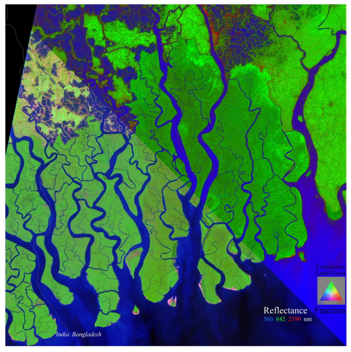
Reflectance\Fraction composites of post-monsoon Sentinel 2 HLS for jd 322 of 2018. Spectral unmixing of the HLS reflectance by inversion of a 3 endmember linear spectral mixture model using standardized spectral endmembers projects the 11 reflectance bands onto a ternary land cover space to yield per-pixel fractional abundance estimates of sediment and soil Substrate, illluminated Vegetation and Dark fractions of water or shadow. The diagonal split illlustrates the effectiveness of the ternary mixture model by greater separation of primary colors as physically distinct land cover components.
Figure 3.
Reflectance\Fraction composites of post-monsoon Sentinel 2 HLS for jd 322 of 2018. Spectral unmixing of the HLS reflectance by inversion of a 3 endmember linear spectral mixture model using standardized spectral endmembers projects the 11 reflectance bands onto a ternary land cover space to yield per-pixel fractional abundance estimates of sediment and soil Substrate, illluminated Vegetation and Dark fractions of water or shadow. The diagonal split illlustrates the effectiveness of the ternary mixture model by greater separation of primary colors as physically distinct land cover components.

Figure 4.
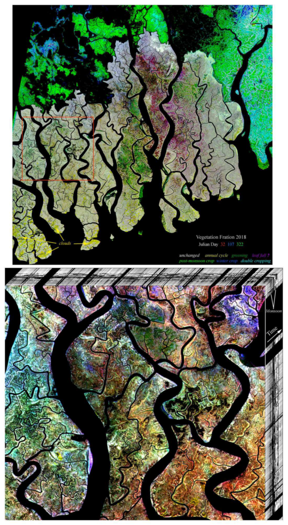
Tri-temporal vegetation maps. HLS Sentinel 2 vegetation fractions from julian days 32 (r), 107 (b) and 322 (g) of 2018 with common linear stretch (top) show spatially coherent seasonal greenness variations of ± 20% in mangroves and much larger changes in agricultural fields. A 10 x10 km substack from western edge (inset & bottom) shown as a spatiotemporal cube has more subdued, but still spatially coherent, temporal greenness variations on tri-temporal composite (front of cube) while seasonal progression of 69 HLS vegetation fraction maps (top & right edges) clearly show variations in post-monsoon greening. The Gaussian stretch of the tri-temporal substack reveals even finer scale coherent variations in seasonal greenness.
Figure 4.
Tri-temporal vegetation maps. HLS Sentinel 2 vegetation fractions from julian days 32 (r), 107 (b) and 322 (g) of 2018 with common linear stretch (top) show spatially coherent seasonal greenness variations of ± 20% in mangroves and much larger changes in agricultural fields. A 10 x10 km substack from western edge (inset & bottom) shown as a spatiotemporal cube has more subdued, but still spatially coherent, temporal greenness variations on tri-temporal composite (front of cube) while seasonal progression of 69 HLS vegetation fraction maps (top & right edges) clearly show variations in post-monsoon greening. The Gaussian stretch of the tri-temporal substack reveals even finer scale coherent variations in seasonal greenness.

Figure 5.
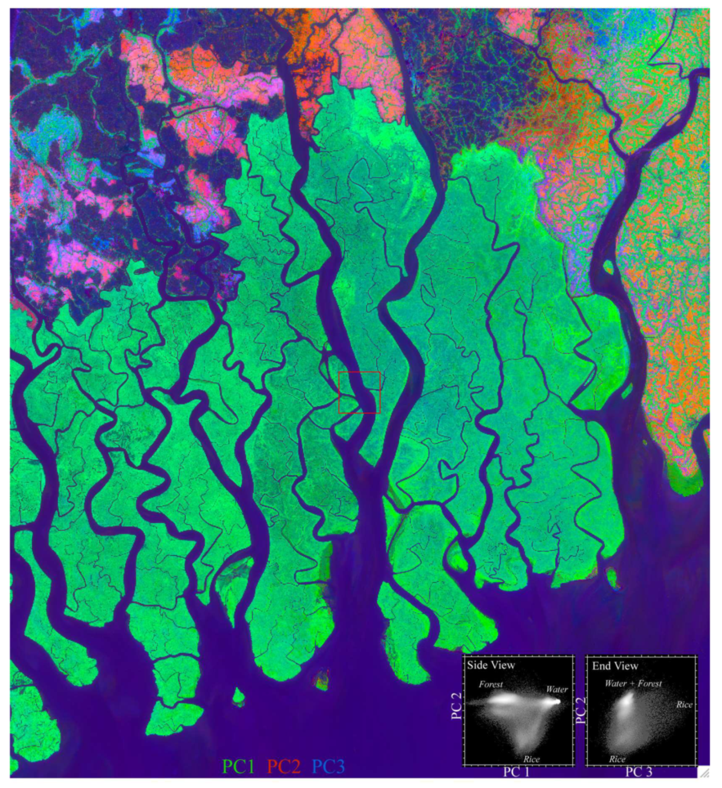
Low order PC composite of HLS S30 vegetation fraction time series. The inset temporal feature space shows clusters distinguishing mangrove forest from rice fields from water bodies. The wide variety of rice phenologies produces a 3D continuum encompassing more of the feature space than the forest-water continuum and compressing the forest into two closely packed clusters in one apex of the feature space. As a result, the forest appears only shades of green but the rice paddys appear a variety of colors corresponding to varying combinations of PCs 1, 2 & 3.
Figure 5.
Low order PC composite of HLS S30 vegetation fraction time series. The inset temporal feature space shows clusters distinguishing mangrove forest from rice fields from water bodies. The wide variety of rice phenologies produces a 3D continuum encompassing more of the feature space than the forest-water continuum and compressing the forest into two closely packed clusters in one apex of the feature space. As a result, the forest appears only shades of green but the rice paddys appear a variety of colors corresponding to varying combinations of PCs 1, 2 & 3.

Figure 6.
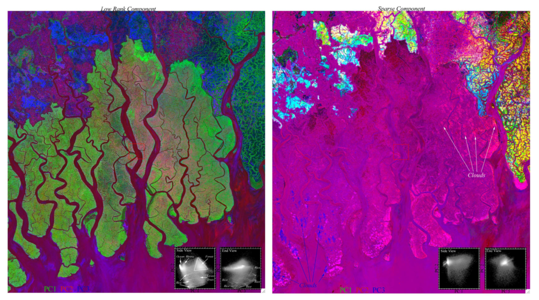
Low order PC composites of RPCA Low Rank and Sparse component HLS S30 vegetation fraction time series. The Low Rank temporal feature space (inset left) clearly separates water from vegetation but also multiple rice phenologies from levee trees from mangrove forest. The Sparse Component contains more transient features like clouds, river sediments and finer scale rice phenology on polders to the north and east of the forest.
Figure 6.
Low order PC composites of RPCA Low Rank and Sparse component HLS S30 vegetation fraction time series. The Low Rank temporal feature space (inset left) clearly separates water from vegetation but also multiple rice phenologies from levee trees from mangrove forest. The Sparse Component contains more transient features like clouds, river sediments and finer scale rice phenology on polders to the north and east of the forest.

Figure 7.
Temporal mixture model fraction map for HLS Low Rank image time series. Inset temporal EMs correspond to apexes of the mangrove cluster in the PC1/2 temporal feature space shown in Figure 6. Water and agricultural areas appear blue and magenta because they lie outside the model but closest to the blue EM. Note qualitative spatial similarity to the tri-temporal fraction map in Figure 4. The red EM shows a decrease in greenness preceding the monsoon, but little increase after.

Figure 8.
Temporal feature space and PC map of 10 × 10 km substack from Figure 4. The PC map shows spatially coherent structure resulting from distinct combinations of PCs 1–3. The feature space (bottom) clearly separates water from forest, spanning 3 distinct senescent phenologies at apexes of PC 3/2 space.

Figure 9.
S2 HLS phenology map for 10 × 10 km substack with WorldView-2 comparison. The phenology map (top) is derived from the temporal mixture model based on the 3 tEMs spanning the temporal feature space in Figure 8. Water lies off the model plane but projects onto the slower senescent tEM so can be distinguished by higher model misfit. Comparison with 2010 WorldView-2 image (bottom) shows clear correspondence between phenology fractions and canopy density. The more open canopy areas show more shadow and exposed mud consistent with lower vegetation fractions in the corresponding tEMs in Figure 8. © Worldview-2, Digital Globe 2019.

Figure 10.
Interannual temporal feature space and endmembers for 1989–2017 annual post-monsoon Landsat vegetation fraction time series. Most profound changes in vegetation cover are related to advance and retreat of shorelines, riverbanks and channel networks. Bank erosion can occur quickly, but most changes are progressive over multiple years with vegetation thinning gradually or mudflat colonization occurring by vegetation species succession. Multi-year loss and recovery are less common, but do occur in some areas.

Figure 11.
Interannual change map for Southeastern Bangladesh Sundarban 1989–2017. PC1 shows mean vegetation abundance while warmer and cooler colors show decadal increase and decrease of vegetation respectively. Shoreline and riverbank retreat from erosion are pervasive, particularly along the wider channels. Vegetation colonization of mudflats is more conspicuous but accounts for less area than is lost to erosion.

Figure 12.
Impact and recovery from Cyclone Sidr on 11.11.2007. Mean vegetation fraction from forest south and west of 22.2°N 89.9°E (cross) drops 0.08 immediately after Sidr but recovers almost fully to its long-term mean of 0.20 (including shadow & water) by the following year. The area of mangrove defoliation (brown on 30.11.2007) is localized to a NNE-SSW swath immediately west of the cyclone track. Defoliation and erosion was most pronounced along south-facing shorelines (top) but measurable shoreline retreat was more focused.

© 2019 by the authors. Licensee MDPI, Basel, Switzerland. This article is an open access article distributed under the terms and conditions of the Creative Commons Attribution (CC BY) license (http://creativecommons.org/licenses/by/4.0/).
Share and Cite
MDPI and ACS Style
Small, C.; Sousa, D. Spatiotemporal Characterization of Mangrove Phenology and Disturbance Response: The Bangladesh Sundarban. Remote Sens. 2019, 11, 2063. https://0-doi-org.brum.beds.ac.uk/10.3390/rs11172063
AMA Style
Small C, Sousa D. Spatiotemporal Characterization of Mangrove Phenology and Disturbance Response: The Bangladesh Sundarban. Remote Sensing. 2019; 11(17):2063. https://0-doi-org.brum.beds.ac.uk/10.3390/rs11172063
Chicago/Turabian StyleSmall, Christopher, and Daniel Sousa. 2019. "Spatiotemporal Characterization of Mangrove Phenology and Disturbance Response: The Bangladesh Sundarban" Remote Sensing 11, no. 17: 2063. https://0-doi-org.brum.beds.ac.uk/10.3390/rs11172063
Note that from the first issue of 2016, this journal uses article numbers instead of page numbers. See further details here.