Article

Integrating SEBAL with in-Field Crop Water Status Measurement for Precision Irrigation Applications—A Case Study

1
Department of Agronomy, Food, Natural resources, Animals and Environment (DAFNAE), Università degli Studi di Padova, 35020 Legnaro, Italy
2
Centrale Valutativa Srl, 00131 Roma, Italy
*
Author to whom correspondence should be addressed.
Remote Sens. 2019, 11(17), 2069; https://0-doi-org.brum.beds.ac.uk/10.3390/rs11172069
Submission received: 31 July 2019 / Revised: 25 August 2019 / Accepted: 30 August 2019 / Published: 3 September 2019

Abstract

:
The surface energy balance algorithm for land (SEBAL) has been demonstrated to provide accurate estimates of crop evapotranspiration (ET) and yield at different spatial scales even under highly heterogeneous conditions. However, validation of the SEBAL using in-field direct and indirect measurements of plant water status is a necessary step before deploying the algorithm as an irrigation scheduling tool. To this end, a study was conducted in a maize field located near the Venice Lagoon area in Italy. The experimental area was irrigated using a 274 m long variable rate irrigation (VRI) system with 25-m sections. Three irrigation management zones (IMZs; high, medium and low irrigation requirement zones) were defined combining soil texture and normalized difference vegetation index (NDVI) data. Soil moisture sensors were installed in the different IMZs and used to schedule irrigation. In addition, SEBAL-based actual evapotranspiration (ETr) and biomass estimates were calculated throughout the season. VRI management allowed crop water demand to be matched, saving up to 42 mm (−16%) of water when compared to uniform irrigation rates. The high irrigation amounts applied during the growing season to avoid water stress resulted in no significant differences among the IMZs. SEBAL-based biomass estimates agreed with in-season measurements at 72, 105 and 112 days after planting (DAP; r2 = 0.87). Seasonal ET matched the spatial variability observed in the measured yield map at harvest. Moreover, the SEBAL-derived yield map largely agreed with the measured yield map with relative errors of 0.3% among the IMZs and of 1% (0.21 t ha−1) for the whole field. While the FAO method-based stress coefficient (Ks) never dropped below the optimum condition (Ks = 1) for all the IMZs and the uniform zone, SEBAL Ks was sensitive to changes in water status and remained below 1 during most of the growing season. Using SEBAL to capture the daily spatial variation in crop water needs and growth would enable the definition of transient, dynamic IMZs. This allows farmers to apply proper irrigation amounts increasing water use efficiency.

1. Introduction

Agriculture is a major and inefficient consumer of fresh water and the competition with other sectors for water is likely to increase exponentially in the next decades [1]. For this reason, a more reasonable and efficient use of water in agriculture is a crucial aspect in order to meet the food needs of the rapidly increasing world population [2,3].
Variable rate irrigation (VRI) has been demonstrated to provide better water use efficiency (WUE) while increasing crop yields [4,5,6]. VRI systems are today integrated with a wide variety of information in order to define proper rates for each irrigation management zone (IMZ), ranging from soil moisture sensing to thermal imagery [7,8,9,10].
Crop evapotranspiration (ETc) is an important factor in estimating crop water demand and has been used to estimate yields and schedule irrigation [8,11]. Commonly, ETc from agricultural areas is calculated by multiplying the reference evapotranspiration (ET0; [12]) by a constant crop coefficient without considering the possible ETc spatial variations in water or nutrient-limited zones ([13]).
Energy balance techniques [14,15,16,17] have been extensively used to map evapotranspiration at the local or regional scale through satellite-based image-processing tools such as the surface energy balance algorithms for land (SEBAL; [18]) and mapping evapotranspiration at high resolution with internalized calibration (METRIC™; [13]). These approaches have been tested under different soil and climate conditions in more than 30 countries worldwide [19,20,21,22] with typical field scale accuracy in ET estimates ranging between 85% for one single-day events up to 95% on a seasonal basis [20].
SEBAL estimates the evapotranspiration component converting the sensed satellite radiances (visible, near infrared and thermal-infrared) into surface parameters such as surface temperature, surface albedo, and normalized difference vegetation index (NDVI). The different components of the energy balance equation are then calculated using these surface parameters [13]. SEBAL’s main advantages are (i) limited input data required, (ii) it estimates ET without a priori knowledge on soil, crop and management conditions (no land use classification required), (iii) it is based on a physical concept, applicable for various climates and (iv) it can be applied at different spatial and temporal resolution [18].
While remote sensing-based energy balance techniques (e.g., SEBAL) have been extensively used to map evapotranspiration at different scales with interesting results [21,22], the effort in using remotely sensed data to evaluate water management practices and schedule irrigation has been limited. Some authors [23] argued the temporal and spatial resolution of currently available remote sensing data are not sufficient to use actual evapotranspiration estimates for on-farm research. Typical turnaround time for satellite image acquisition and processing is between one and three weeks [23], whereas ET maps should be delivered almost in real-time to correctly use the remotely sensed information for irrigation scheduling. Moreover, the spatial resolution of ET maps calculated applying remote sensing-based energy balance techniques frequently does not match with spatial resolution requested for VRI.
However, data fusion, sub-pixel extraction [23] and temporal integration techniques [24,25,26] could represent an alternative to improve both spatial and temporal resolution. The availability of new satellite platforms with higher temporal and spatial resolution is a need for a better deployment of these models. In addition, evapotranspiration estimates need to be validated by means of well-established methods, such as soil moisture sensing, shown to be a strong indicator of plant water status in order to define specific irrigation thresholds [10].
The objective of this study is to calculate SEBAL-based actual ET estimates in a pivot-irrigated field in North-Eastern Italy and compare the results to soil moisture data and crop stress coefficients (Ks). Accuracy of the SEBAL results is then assessed by comparing spatially distributed biomass and crop yield measurements.

2. Materials and Methods

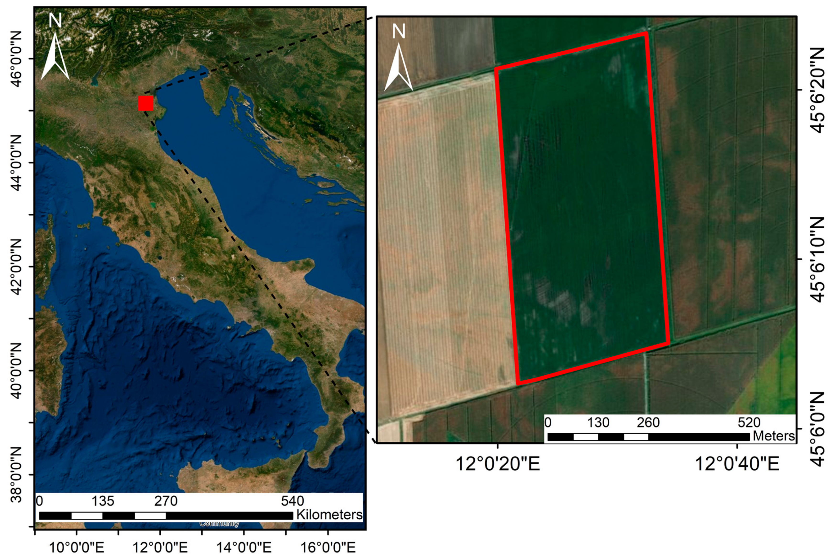
2.1. Study Area and Plant Material

To validate SEBAL-based ET and biomass estimates, a study was conducted on a pivot-irrigated, 16-ha field located in Pettorazza Grimani, Italy (45°6′7.19″N, 12°0′45.51″E; Figure 1). Maize (Zea mais L.) seeds of PR32B10 (Pioneer Hi-Bred International, Inc., Johnston, IA, USA) variety were planted on April 13th, 2015 at 0.45 m inter-row spacing and seeding rate of 8 seeds m−2. Prior to planting, cultivation operations included an autumn plowing at 30 cm depth and a seedbed preparation carried out by using a spring tine cultivator. Fertilization included a base-dressing of 65 kg N ha−1 with manure, 92 kg P2O5 ha−1, 111 kg K ha−1 K2O before the autumn plowing and a top-dressing of 184 kg N ha−1 (urea). Maize was harvested on September 7th, 2015.

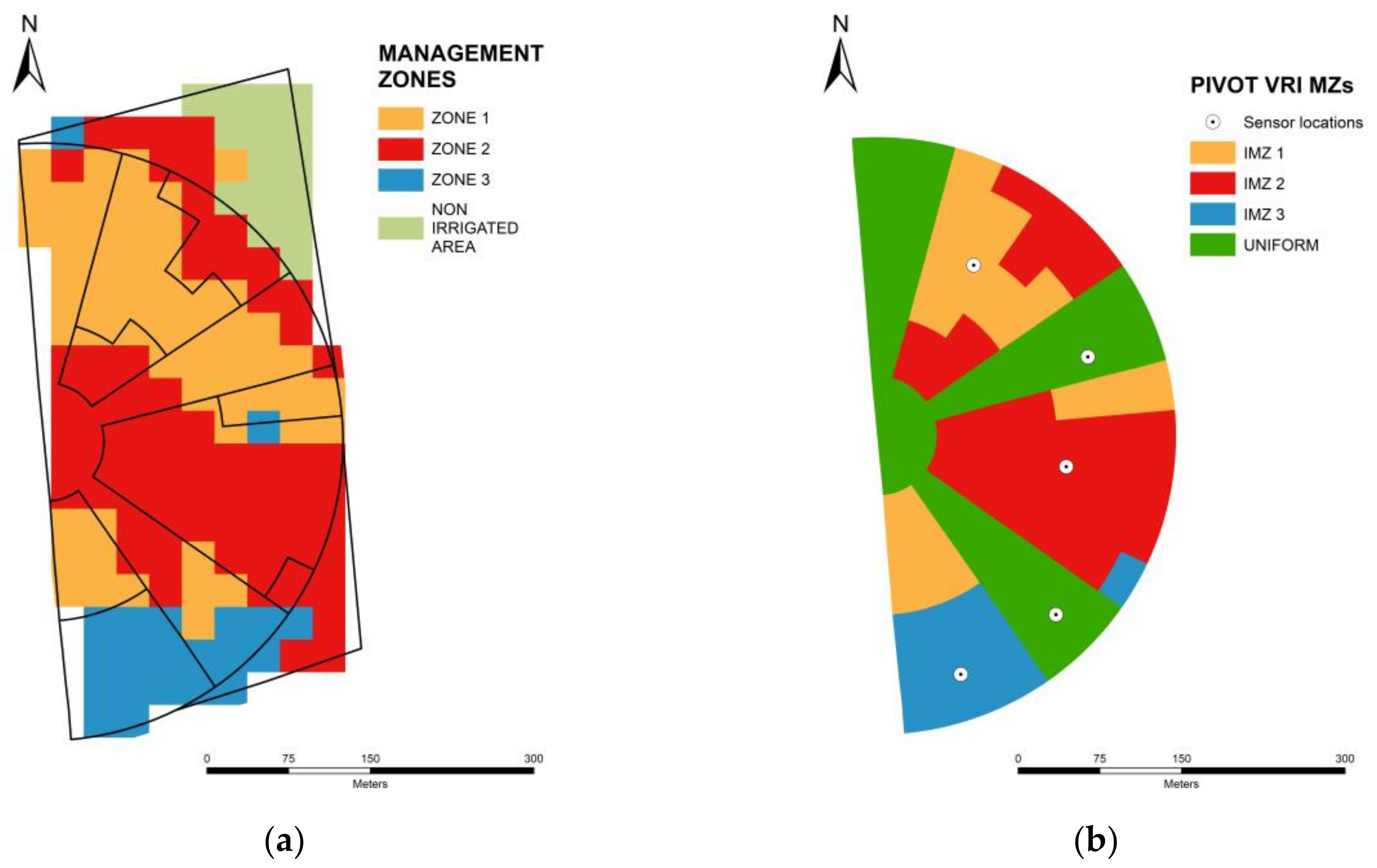
2.2. Soil Sampling and Management Zone Delineation

Irrigation management zones were defined integrating soil texture and NDVI data. A mixed-sampling scheme of the top soil layer (0–0.3 m) was followed based on a regular grid: 55 samples were collected at the nodes of 55 m × 65 m grids and 48 additional points at the nodes of 16 transects at 2.5, 15 and 30 m from each randomly chosen grid node, resulting in a total of 103 samples (Figure 2a; [27]). Soil texture was determined for all the 103 disturbed soil samples (Figure 2b,c) using a Malvern Mastersizer 2000 (Malvern Instruments Ltd, Great Malvern, UK) laser particle size analyzer (see Supplementary Materials for texture analysis method) and spatially interpolated using ordinary kriging. Maize spatial variability in NDVI was estimated at the peak of plant vigor (tasseling/silking growth stage) from previous seasons using LANDSAT 7 images of June 29th, 2009 and June 24th, 2013 [28]. LANDSAT 7 images were selected since they have the same spatial resolution as the VRI center pivot (30 m x 30 m pixels). Moreover, these images were selected since they represented the maize variability in NDVI during two extremely different growing seasons: A rainy (2009) and a dry (2013) year.
The investigated area was then divided into three IMZs based on the management zone analyst 1.0’s fuzziness performance index (FPI) and the normalized classification entropy (NCE) [29]. As discussed in [29], the optimal number of zones (clusters) was identified when each index had its minimum representing the least membership sharing (FPI) or greatest amount of organization (NCE). In addition, a fourth IMZ was defined and treated as the uniform irrigation zone.

2.3. Soil Moisture Assessment and Variable Rate Irrigation System Assessment

To monitor the soil moisture condition in the field, three 5TE soil moisture sensors (Decagon Devices Inc., Pullman, WA, USA) were installed in each IMZ at three different depths, 0.1, 0.3 and 0.5 m below the soil surface. Each array of soil moisture sensors was connected to an EM50G wireless cellular data logger (Decagon Devices Inc., Pullman, WA, USA). Before field installation, all sensors were calibrated in the laboratory (accuracy of ± 4%; [28]). The sensors collected soil moisture data every 30 min. Data were averaged for each array of sensors to get daily averages for the three different depths and then a unique average for each location. In the three IMZs, irrigation was scheduled when volumetric water content (VWC) approached 35% for zone 1, 32% for zone 2 and 28.5% for zone 3. The specific irrigation thresholds were defined based on soil hydraulic parameters for the different IMZs. Having the zones different soil characteristics, the thresholds were defined accordingly. In the Uniform IMZ, irrigation was applied at the maximum rate (38 mm) each time one of the other IMZs was irrigated.
Irrigation was supplied using a 270-m long, center pivot equipped with a Valley® (Valley Irrigation, Valley, USA) variable rate irrigation system. Each sprinkler was controlled (on or off) by a pneumatically actuated flow control valve. The 96 sprinklers were grouped into 10 zones, each about 25 m in length. The uniformity of the irrigation system was assessed before the beginning of the growing season, following the American Society of Agricultural and Biological Engineers (ASABE) standards and the “catch can” layout proposed by [28,30,31]. The uniformity of application of the conventionally operated pivot (without VRI) was evaluated using the Hermann and Hein (CUHH) uniformity coefficient [32] and the lower quarter distribution uniformity (DUlq) coefficient [30]. The uniformity test resulted in high CUHH and DUld (93.9 and 0.91, respectively). Moreover, measured collector volumes (observed) were compared to the predicted volumes (expected) [33] in order to test the performance of the VRI system. The application rates were set at 50%, 60%, 70%, 80% and 90% of the maximum pivot rate (30 mm). The catch cans were placed following two patterns, transect and arc-wise. Root mean square error (RMSE) of 1.7 and r2 = 0.86 highlighted a good fit between expected and observed rates [28].

2.4. Evapotranspiration, Biomass and Yield Estimates Using the Surface Energy Balance Algorithm for Land (SEBAL)

The surface energy balance algorithm for land (SEBAL) determines the actual evapotranspiration (ETr) of each pixel by solving the energy balance equation (Equation (1); [18]):
λ E = R n G 0 H ,
where Rn is the net radiation, λE is the latent heat flux, G0 is the soil heat flux and H is the sensible heat flux.
Rn is calculated from surface reflectance and surface temperature, the soil heat flux (G0) as a function of Rn, surface temperature and NDVI. H is considered proportional to the ratio between the surface-air temperature difference (dT) and bulk aerodynamic resistance (rah) [18,24]. SEBAL computes the sensible heat flux H through a “calibration” procedure where dry (Rn = H + G0, thus λEdry ~ 0) and wet (Rn = G0 + λE, Hwet ~ 0) pixels are selected and used to calculate the vertical temperature difference (ΔT) required to match the variation in H between the dry and wet pixels [26]. The wet pixel was identified as a very well watered crop pixel (low temperature, low albedo and high NDVI) and the dry pixel was searched between poorly vegetated or base soil areas with high temperature, high albedo and low NDVI.
Therefore, SEBAL calculates the evaporative fraction (Λ) considering the H and λE components ([18]; Equation (2)).
Λ = λ E R n G 0 = R n G o H R n G o
Moreover, the evaporative fraction (Λ) is assumed to be constant throughout the day. In fact, the difference between the Λ at the moment of image collection and the 24-h Λ average is considered as non-significant [24,26].
The latent heat flux λE is then calculated multiplying the Λ by the diurnal net radiation (Rn24h) as in Equation (3):
λ E = Λ × R n 24 h .
Landsat 7 and 8 satellite images from April 19th, May 14th and 29th, June 6th and 30th, July 8th, 16th and 24th, August 9th and 17th, and September 2nd, 2015 were downloaded and automatically processed using a web-based platform called Tethys (Centrale Valutativa s.r.l.) to estimate the energy balance components. All dates had favorable clear-sky weather conditions. Visible bands (bands 1, 2, 3, 4, 5 and 7) were used for albedo (α), and vegetation index calculations. Thermal band (band 6) was used for surface temperature (Ts) and sensible heat (H). The spatial resolution was 30 m × 30 m on the visible bands and 60 m × 60 m on the thermal band. An atmospheric correction was performed to convert the top-of-atmosphere (TOA) radiance into surface reflectance using the second simulation of satellite signal in the solar spectrum algorithm (6S; [34]).
To overcome the lack of satellite images on a daily basis, actual evapotranspiration (ETr) was calculated for each of the aforementioned satellite image acquisition dates. Then, ETr on the date j was divided by the reference evapotranspiration (ET0) on the same date j to calculate the fraction ETrFj. ET0 was estimated using the FAO-56 method (Penman–Monteith equation) [35]. The fraction ETrFj = ETr/ET0 was then considered constant for the time period between j and the successive acquisition date j + 1 [24,26]. Seasonal actual evapotranspiration (ETseasonal) was then calculated using Equation (4).
E T s e a s o n a l = j ( E T r F j × i = t j t j + 1 E T 0 i ) ,
where tj and tj + 1 represents the time period between two consecutive image acquisition dates.
Maize aboveground biomass production (in kg ha−1 day−1) for each pixel of the satellite images was calculated from Tethys using the fraction of absorbed photosynthetically active radiation (fPAR) = absorbed PAR (APAR)/total PAR (PAR), the evaporative fraction (Λ) and light use efficiency (e’). fPAR was estimated from NDVI values as shown in Equation (5) [17]:
f P A R = 0.161 + 1.257 × N D V I .
The light use efficiency factor was set at 4 g/MJ [34]. Total biomass (BIO) production was converted into total above-ground biomass as total biomass (BIO) × 0.77 (Equation (6); [17]).
B I O = e × Λ × f P A R × 0.84 .
Maize yield was obtained multiplying the total aboveground biomass for each of the irrigation management zones by a specific harvest index (HI) factor equal to 0.5. Measured and SEBAL-derived yield averages were also calculated for each IMZ, uniform zone and for the rainfed portion of the field (top right corner). Moreover, differences between the measured and SEBAL-estimated yield were calculated for each pixel as in Equation (7):
D e l t a = S E B A L   y i e l d o b s e r v e d   y i e l d o b s e r v e d   y i e l d × 100 .

2.5. Crop Growth Data

To monitor crop growth during the season, biomass samples were collected on three sampling dates, at 72 (June 24th, 2015), 102 (July 24th, 2015) and 115 (August 6th, 2015) days after planting (DAP). On each sampling date, two 1 m2 sections were destructively harvested for each IMZ. The biomass was then dried for 24 h in a forced-air oven to determine the total above-ground dry weight (DW) in kg ha−1.
Yield data was collected at harvest using a New Holland CR8080 (New Holland Agriculture, Italy) combine harvester equipped with a yield monitor (grain mass flow and moisture sensor) and a differential global positioning system (DGPS). The harvester had a 7.5 m header and collected yield data every second. Raw data, expressed as 14% grain moisture content, was imported using SMS™ Advanced (AgLeader Technology, Ames, USA), cleaned to exclude field-edge effect and low yield values due to combine maneuvers and expressed as dry matter per hectare (DM ha−1). The combine-derived data points were interpolated and resampled at 30 m × 30 m to match the spatial resolution of the SEBAL yield map.

2.6. SEBAL-Based and Soil Moisture Data-Based Water Stress Coefficient

Water stress coefficients (Ks) were calculated for each soil moisture sensor location using the moisture data collected at the three different depths. Water content at −33 KPa (field capacity) and −1500 KPa (permanent wilting point) were estimated from the soil characteristics of each IMZ using the “Rosetta” model [36]. Soil moisture-based Ks was then calculated on a daily basis using the FAO-56 method as follows [12]:
K s = T A W D r R A W ,
where TAW (mm) is the total available soil water in the root zone, Dr (mm) is root zone depletion and RAW is the fraction of the TAW that a crop can extract from the root zone before reaching water stress (RAW assumed 0.5 × TAW).
The SEBAL-based Ks (Ks SEBAL) was calculated by extracting the SEBAL actual Kc (Kc SEBAL) for each sensor location on a daily basis. Therefore, Ks SEBAL was divided by the basal crop coefficient to estimate the specific Ks (Equation (9)).
K s   S E B A L = K c S E B A L K c b ,
where Kcb is the basal crop coefficient estimated according to the FAO method [35] and Kcsebal is the actual crop coefficient calculated from SEBAL.
Ks SEBAL is assumed to be equal to 1 when Kcsebal ≥ Kcb. The Ks values were compared over the irrigation season to investigate a possible relationship between the two methods and the sensitivity of Kc SEBAL in capturing water stress-related changes in evapotranspiration.

2.7. Statistical Analyses

A regression analysis was used to evaluate SEBAL performances in estimating the biomass collected on the aforementioned sampling dates. The coefficient of determination was also calculated to describe the proportion of the total variance described by the model.

3. Results

3.1. Irrigation Management Zones (IMZs) Delineation

The field presented high variability in soil texture moving along the north-south axis with coefficient of variation of 25% for sand and 23% for clay. The sandy areas were located in the southern part while the north part of the field had high clay content (Figure 2). NDVI maps were strongly dependent on the season with the sandy areas showing high NDVI values in rainy seasons as in the 2009 map (Supplementary Materials Figure S1) and low values in dry seasons (2013 map, Supplementary Materials Figure S1) [28]). Soil texture (sand and clay; Figure 2) and NDVI data were integrated in order to delineate the IMZs using the aforementioned Management Zone Analyst software. The optimal number of management zones was selected based on the fuzziness performance index (FPI) and the normalized classification entropy (NCE) indices as shown in Figure 3 [29]. The cluster analysis identified a total of four zones but only the three IMZs under the pivot-irrigated area were considered for the experiment (Figure 4a): Zone 1, located in the north-eastern part of the field, was characterized by silty loam texture; Zone 2, located in the central part of the field, by loam texture, and Zone 3, in the south-western part of the field, by sandy-loam texture. The irrigation application map (Figure 4b) was developed matching the aforementioned management zones (zone 1, 2 and 3), and a fourth, uniform irrigated area to the resolution of the center pivot. The application map was then downloaded to the VRI controller and used for every irrigation event.

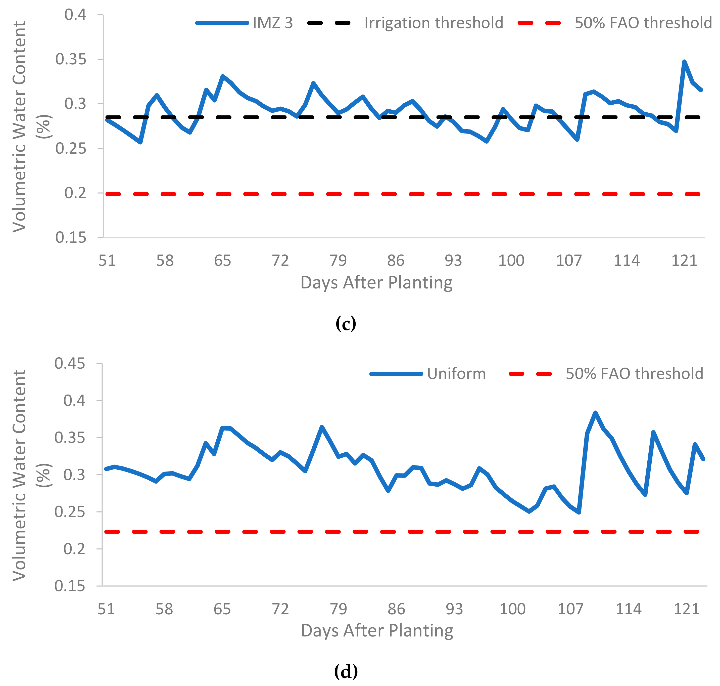
3.2. Soil Moisture Data and Irrigation Prescriptions

In 2015, rainfall totaled 272.8 mm between planting and harvest (Figure 5). The growing season was characterized by a dry April, July, August, September and a wet period between June and July. Total irrigation rates applied for each IMZ and the uniform zone are presented in Table 1 [28]. The high water demand during the growing reason resulted in a progressive decrease of the VWC below field capacity from mid-July (93 DAP) to the beginning of August, since the time required from the pivot for a complete rotation was the limiting factor (Figure 6).
As discussed before, irrigation was triggered when VWC approached 35% for zone 1, 32% for zone 2 and 28.5% for zone 3 (black dotted lines reported in Figure 6). Moreover, VRI allowed water saving of 8 mm (IMZ 1) and 42 mm (IMZ 3) throughout the season when compared to uniform irrigation rates, while IMZ 2 totaled the same amount of water supplied in the uniform zone (Table 1).

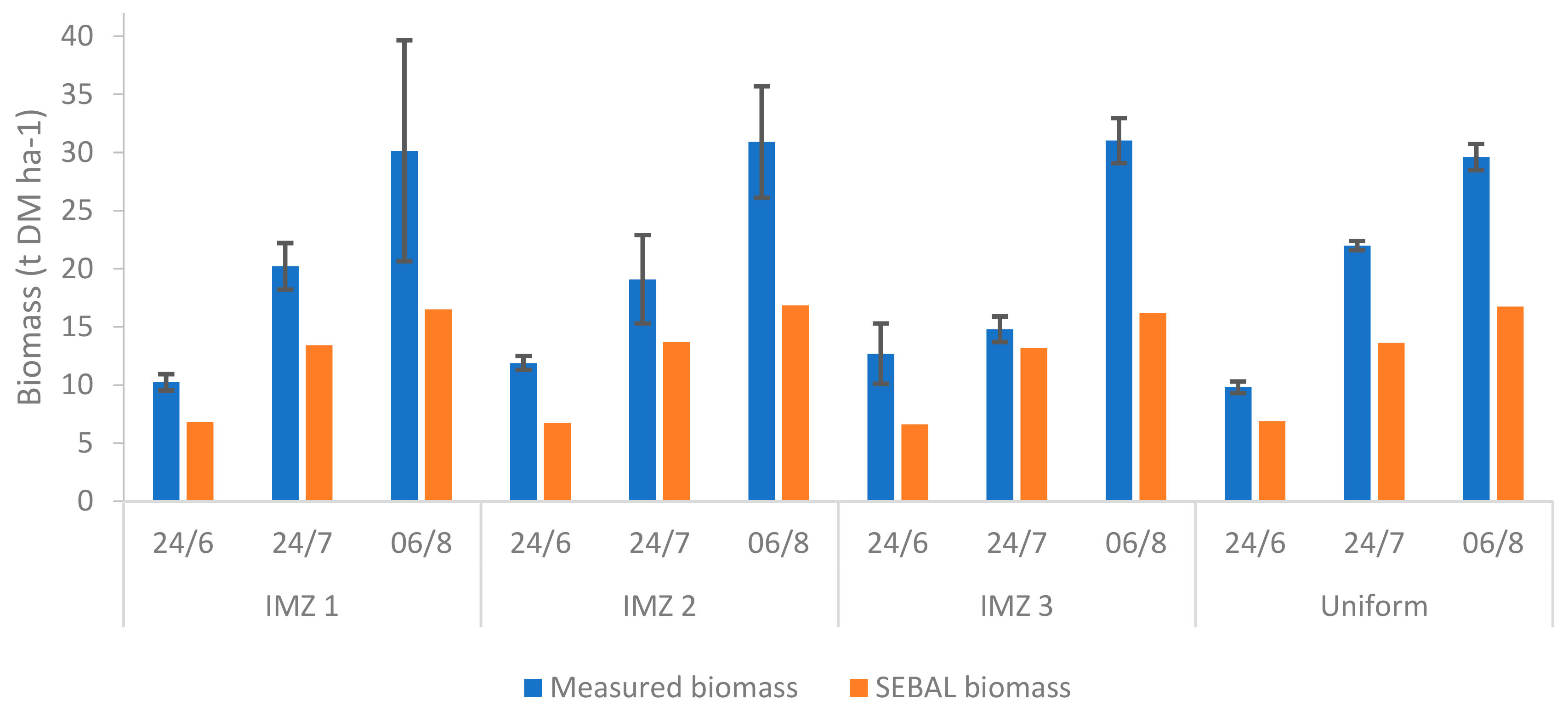
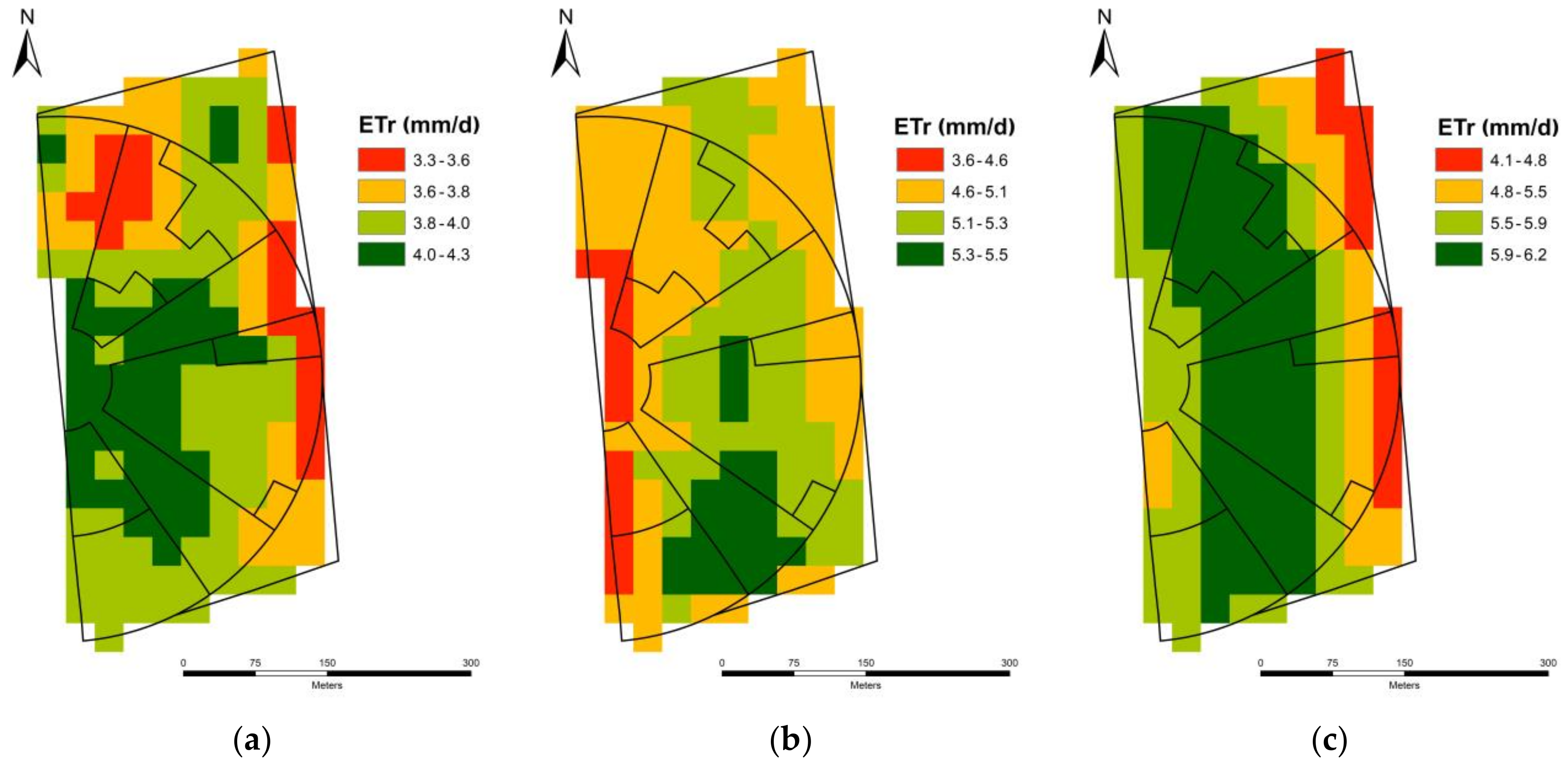
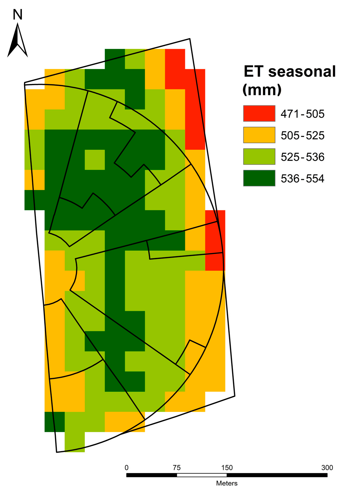
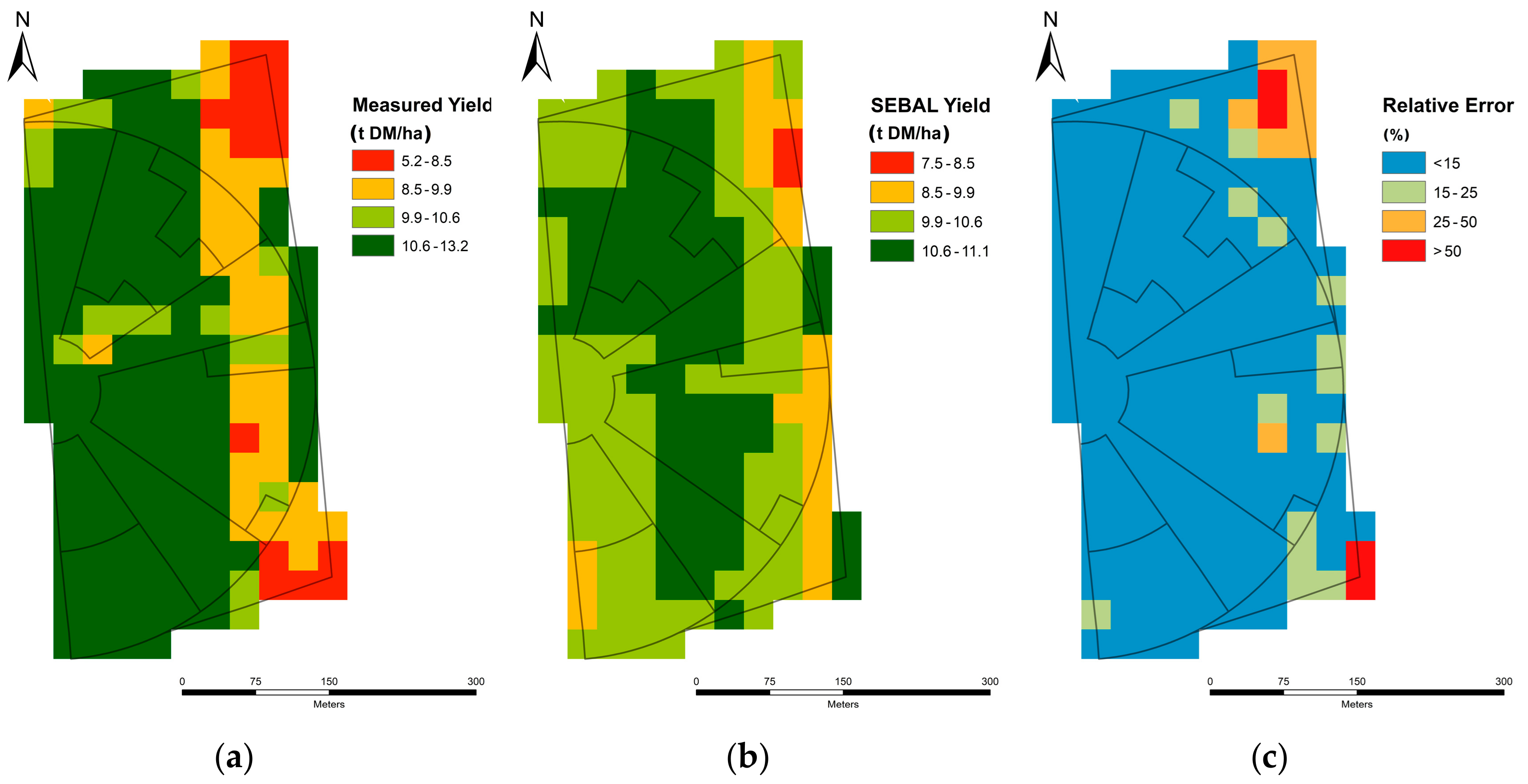
3.3. Measured and SEBAL-Based Data

Figure 7 shows the maize biomass values in t DM ha−1 hand harvested for each IMZ on the three aforementioned sampling dates (blue bars). The high irrigation amounts applied during the growing season to avoid water stress in the experimental area resulted in no significant differences among the four irrigation zones. SEBAL-based biomass values extracted from the sensor locations at 72, 102 and 115 DAP resulted in a good agreement with observed data (r2 = 0.87, Supplementary Materials Figure S2). However, as shown in Figure 7, SEBAL considerably underestimated the measured biomass at every sampling date. This underestimation in biomass could be related to the different spatial resolutions of the two systems: While biomass samples were collected on a 1 m2 sections, SEBAL provided biomass estimates on 30 m pixels × 30 m pixels.
SEBAL-derived ETr maps on June 2nd, July 2nd and August 6th (Figure 8) exhibited a marked temporal variation across the field (NDVI maps used to calculate ETr are shown in Supplementary Materials Figure S3). While early season ETr maps as June 2nd, 2015 presented a limited variability in ET with values ranging between 3.4 and 4.3 mm/d (Figure 8a), late in the season the variability increased as in the case of August 6th, 2015 (Figure 8c) with ET values between 4.0 and 6.2 mm/d. In general, the central part of the field had greater ETr values and the right-hand part had low ETr.
This is confirmed from the seasonal (April 13th to September 7th) evapotranspiration map (ETseasonal; Figure 9). Seasonal ET ranged between 471 mm to 554 mm with the lowest values in the top right part of the field and the highest values in the central area. ETseasonal map largely matches the spatial variability of the measured yield map, with high seasonal ET associated with high yielding zones and low ET characterizing the low yielding zones (Figure 10a).
The SEBAL-based yield map (Figure 10b) had a similar spatial pattern when compared to the measured yield map. Measured yield values ranged between 5.2 to 13.2 t ha−1, whereas SEBAL yield ranged between 7.5 to 11.1 t ha−1. In both maps, low maize yields were generally observed in the right-hand part of the field, with the lowest yielding area at the top right corner. Moreover, a relative error map was generated as the difference between measured and SEBAL yield values on a pixel basis (Figure 10c). Almost all the pixels with relative errors higher than 25% are located outside the pivot-irrigated area in the rainfed portion of the field, indicating actual biomass or harvest index (HI) could have been overestimated. However, more than 75% of the map presented relative errors lower than 25% between measured and SEBAL yields with most of the pixels having errors below 15%. At the whole field, SEBAL underestimated the measured yield by less than 1 % (0.21 t DM ha−1), which represents an excellent performance in agreement with [37].
In addition, measured and SEBAL yield were averaged at the IMZ scale, considering also the rainfed part of the field (top right corner; Table 2). Measured yield averages between 10.47 and 10.92 t ha−1 in the irrigated areas and 9.39 t ha−1 in the rainfed portion. Differences in yield were not significant between the VRI and the uniform irrigated areas, however, VRI resulted in water savings up to 42 mm as mentioned in 3.2. SEBAL was in a good agreement with measured data, slightly underestimating yield in IMZ 1, IMZ 2 and uniform zone, between −1.9% and −3.6%, and overestimating yield (0.8%) in IMZ 2. A 6.4% overestimation was observed in the rainfed zone. Overall, SEBAL underestimated the total yield by 0.3%, which represents again an excellent result.

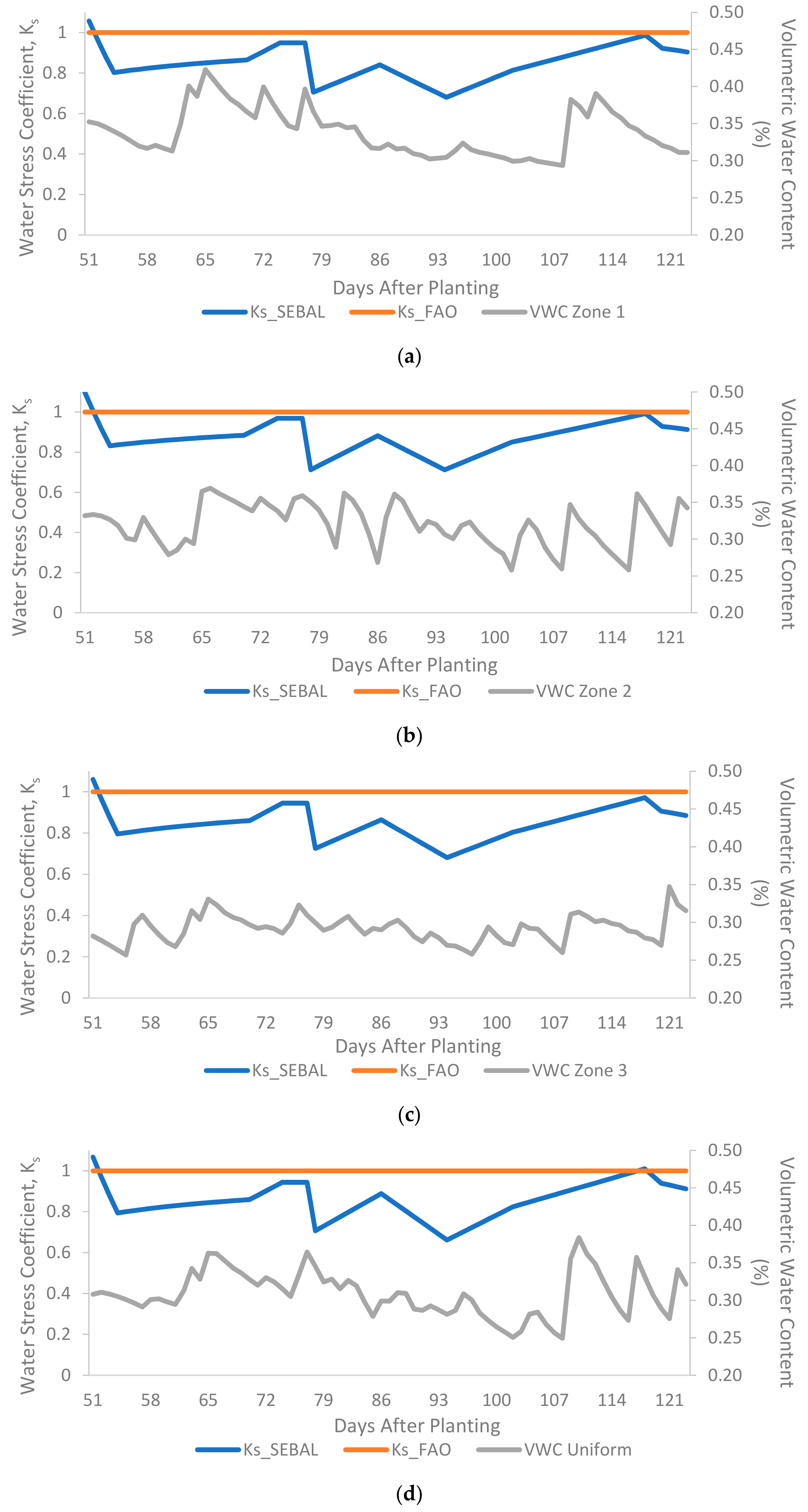
3.4. SEBAL and Soil Moisture-Based Ks

The water stress coefficient (Ks) was used to estimate possible reduction in the potential evapotranspiration over the season. Daily Ks were calculated using the previously described FAO method and the SEBAL actual evapotranspiration. Figure 11 shows the FAO Ks (orange lines) and the SEBAL-based Ks (blue lines) values calculated for all the IMZs and the uniform area.
VWC never exceeded the FAO 50% TAW threshold in all the management zones (Figure 6) and in consequence FAO Ks was always equal to 1 [36]. Conversely, the SEBAL Ks showed changes over the growing season in all the management zones with values frequently lower than the optimum Ks = 1. Moreover, the trend in SEBAL Ks resulted similar in all the zones probably because of the high frequency of irrigation events allowed to maintain the crop well watered irrespectively of the soil variability.

4. Discussion

Weather conditions observed during the summer, did not allow us to fully exploit the VRI potentials. Indeed, exceptionally high temperatures and prolonged drought were observed starting before maize flowering to mid-August. These conditions smoothed the differences between IMZs in terms of water retention capabilities and, as a consequence, between irrigation volumes. Nevertheless, the VRI system coupled with the soil moisture sensors optimized the irrigation scheduling and maximized yields, allowing for fine tuning of the irrigation, particularly in IMZ 1 and IMZ 3. In turn, maize yield did not show any significant differences among the management zones, while water savings compared to the business-as-usual regime ranged from 8 mm (low irrigation requirement zone) to 40 mm (high irrigation requirement zone). In particular, it is worth pointing out that in the sandy area (i.e., IMZ 3), it was possible to obtain a reduction of irrigation volumes, still maintaining yield performances not different from the irrigated control treatment (uniform IMZ).
In the current study we supported the hypothesis that SEBAL estimated parameters such as actual evapotranspiration, crop coefficient and daily biomass accumulation could be used to understand the spatial and temporal variation in the maize water status. Moreover, whether the integration between SEBAL parameters and soil moisture information could represent a viable tool for scheduling irrigation and providing better crop yields while reducing the irrigation amounts.
SEBAL was able to describe 87% of in-field biomass variability, but average data were overestimated with respect to the actual values. These discrepancies could be related to the different spatial resolution between SEBAL and in situ operations. While the former calculated the biomass on a 30 m × 30 m grid, the hand harvested samples were collected on 1 m2 plots. Improving the sampling pattern, collecting a more representative sample for each selected pixel, or using SEBAL parameters with higher spatial resolution could represent possible alternatives to increase the accuracy of estimates on both sides [17].
Conversely, SEBAL-estimated maize yield well correlated to the measured yield map in all the aforementioned management zones but also on a pixel basis (average error less than 1%; 0.21 t ha−1). The relative error map (Figure 10c) reinforces the excellent performance of the algorithm as noted by [37]. Moreover, SEBAL exhibited the highest overestimation of maize yield in the rainfed area (+6.4%). The authors suggest this was probably related to uncertainties in harvest index (HI), which could be affected by plants stress conditions. In fact, the integration of a crop stress-related harvest index model could represent a way to provide better SEBAL-based yield estimates especially for zones under non optimal conditions, as rainfed areas, or when stress periods occur even in irrigated portions over the growing season [38].
ETr and crop coefficient maps calculated by SEBAL, clearly highlight the potentialities of the model to optimize VRI. Unfortunately, it was not possible to compare the accuracy of SEBAL and FAO methods with respect to field ET measurements (e.g., lysimeters and flux towers). As discussed in many other studies, SEBAL resulted in underestimation of ET when compared to the FAO dual coefficient method [19,22,35]. In addition, FAO-56 tabulated Kc and Kcb has been shown to overestimate the observed crop coefficients and ET for humid regions up to 40% [39,40] due to the complexity of the interactions between several soil, weather and plant physiological factors. Moreover, weather conditions (e.g., cloud cover and net radiation) at the time of the satellite overpass and the selection of dry and wet pixels could strongly influence the final ETc values calculated from SEBAL [41,42].
Anyway, SEBAL ETr maps and Ks values showed a marked variability over the growing season even if the FAO method suggested no stress occurred (Ks = 1). While the widely-used FAO method does not account for spatial variability in crop evapotranspiration, the SEBAL ability to use pixel-specific estimates of plant water status represent a promising tool for the definition of transient irrigation management zones as the season moves, thus enabling dynamic variable rate irrigation.

5. Conclusions

In this study, the surface energy balance algorithm for land (SEBAL) was used to map crop evapotranspiration and biomass accumulation and estimate crop yield in a pivot-irrigated maize field. Moreover, SEBAL estimates of crop water stress were coupled with in-season soil moisture sensing data in order to define an irrigation scheduling strategy able to integrate these two approaches. Measured biomass and maize yield values showed a good agreement with SEBAL estimates, indicating the algorithm could be used to provide accurate estimates of crop growth and maize final production. The SEBAL sensitivity to the complex interactions between several soil, weather and plant physiological factors, allowed also to describe the spatiotemporal variability of crop water demands at the field scale. These results suggest that the integration of SEBAL with in-field soil moisture sensing could allow farmers to optimize irrigation scheduling for variable rate irrigation systems, overcoming the simplified FAO single or dual coefficients methods. However, major advancements are still needed for a successful use of SEBAL for irrigation purposes. The specific relationship between SEBAL Ks values and crop water status should be defined in order to identify the proper dynamic variable rate irrigation zones. SEBAL should be coupled with crop simulation models (e.g., DSSAT) to overcome its limited use during long cloudy periods. SEBAL applications should be based on satellites data with higher spatial and temporal resolutions.
Anyway, SEBAL adoption for precision agriculture irrigation will allow us to advance the irrigation science particularly in environments where water availability is scarce or the quality of irrigation water is poor.

Supplementary Materials

The following are available online at https://0-www-mdpi-com.brum.beds.ac.uk/2072-4292/11/17/2069/s1. Figure S1. Comparison between measured biomass and SEBAL biomass estimates in the three irrigation management zones at 72, 102 and 115 days after planting. Figure S2. Normalized Difference Vegetation Index (NDVI) maps from June 29th, 2009 and June 24th, 2013 utilized for the definition of the irrigation management zones in the experimental area. Figure S3. Normalized Difference Vegetation Index (NDVI) maps from April 19th (a), May 14th (b), June 6th (c), July 8th (d), July 24th (e), August 9th (f), 2015 used from the Surface Energy Balance Algorithm for Land (SEBAL) to calculate actual evapotranspiration (ETr).

Author Contributions

Conceptualization, F.M.; methodology, F.M., S.G., L.P., S.L., M.M. and A.B.; software, S.L. and L.P.; formal analysis, S.G.; writing—review and editing, S.G., F.M., M.M. and A.B.

Funding

This research was partially funded by P.S.R 2007-2013-MISURA 214 and the European Space Agency Business Incubation Centre (founded by European Space Agency, Agenzia Spaziale Italiana and Regione Lazio).

Acknowledgments

The authors would to thank Dr Pietro Pietrobelli and Azienda Agricola Eredi Petrobelli Antonio for their assistance during the field experiment.

Conflicts of Interest

The authors declare no conflict of interest. The funders had no role in the design of the study; in the collection, analyses, or interpretation of data, in the writing of the manuscript, or in the decision to publish the results.

References

  1. Hsiao, T.C.; Steduto, P.; Fereres, E. A systematic and quantitative approach to improve water use efficiency in agriculture. Irrig. Sci. 2007, 25, 209–231. [Google Scholar] [CrossRef]
  2. Wallace, J. Increasing agricultural water use efficiency to meet future food production. Agric. Ecosyst. Environ. 2000, 82, 105–119. [Google Scholar] [CrossRef]
  3. Howell, T.A. Enhancing water use efficiency in irrigated agriculture. Agron. J. 2001, 93, 281–289. [Google Scholar] [CrossRef]
  4. O’Shaughnessy, S.A.; Evett, S.R.; Andrade, A.; Workneh, F.; Price, J.A.; Rush, C.M. Site-specific variable-rate irrigation as a means to enhance water use efficiency. Trans. ASABE 2016, 59, 239–249. [Google Scholar]
  5. Vellidis, G.; Liakos, V.; Porter, W.; Tucker, M.; Liang, X. A dynamic variable rate irrigation control system. In Proceedings of the 13th International Conference on Precision Agriculture, St. Louis, MI, USA, 31 July–3 August 2016. [Google Scholar]
  6. Liakos, V.; Porter, W.; Liang, X.; Tucker, M.; McLendon, A.; Vellidis, G. Dynamic Variable Rate Irrigation—A Tool for Greatly Improving Water Use Efficiency. Adv. Anim. Biosci. 2017, 8, 557–563. [Google Scholar]
  7. Vellidis, G.; Tucker, M.; Perry, C.; Reckford, D.; Butts, C.; Henry, H.; Liakos, V.; Hill, R.; Edwards, W. A soil moisture sensor-based variable rate irrigation scheduling system. In Precision Agriculture’13; Springer: Berlin, Germany, 2013; pp. 713–720. [Google Scholar]
  8. Meron, M.; Tsipris, J.; Orlov, V.; Alchanatis, V.; Cohen, Y. Crop water stress mapping for site-specific irrigation by thermal imagery and artificial reference surfaces. Precis. Agric. 2010, 11, 148–162. [Google Scholar]
  9. Chastain, D.R.; Snider, J.L.; Collins, G.D.; Perry, C.D.; Whitaker, J.; Byrd, S.A.; Oosterhuis, D.M.; Porter, W.M. Irrigation scheduling using predawn leaf water potential improves water productivity in drip-irrigated cotton. Crop Sci. 2016, 56, 3185–3195. [Google Scholar]
  10. Snider, J.; Chastain, D.; Porter, W. Plant-based irrigation scheduling. In Linking Physiology to Management; Snider, J., Oosterhuis, D., Eds.; The Cotton Foundation: Cordova, TN, USA, 2015. [Google Scholar]
  11. Bastiaanssen, W.G.; Ali, S. A new crop yield forecasting model based on satellite measurements applied across the Indus Basin, Pakistan. Agric. Ecosyst. Environ. 2003, 94, 321–340. [Google Scholar] [CrossRef]
  12. Allen, R.G.; Pereira, L.S.; Raes, D.; Smith, M. Crop Evapotranspiration-Guidelines for Computing Crop Water Requirements-FAO Irrigation and Drainage Paper 56; FAO: Rome, Italy, 1998; Volume 300, p. D05109. [Google Scholar]
  13. Allen, R.G.; Tasumi, M.; Trezza, R. Satellite-based energy balance for mapping evapotranspiration with internalized calibration (METRIC)—Model. J. Irrig. Drain. Eng. 2007, 133, 380–394. [Google Scholar] [CrossRef]
  14. Teixeira, A.D.C.; Bastiaanssen, W.; Ahmad, M.; Bos, M. Reviewing SEBAL input parameters for assessing evapotranspiration and water productivity for the Low-Middle Sao Francisco River basin, Brazil: Part A: Calibration and validation. Agric. For. Meteorol. 2009, 149, 462–476. [Google Scholar] [CrossRef]
  15. Sun, Z.; Gebremichael, M.; Ardö, J.; De Bruin, H. Mapping daily evapotranspiration and dryness index in the East African highlands using MODIS and SEVIRI data. Hydrol. Earth Syst. Sci. 2011, 15, 163–170. [Google Scholar] [Green Version]
  16. Papadavid, G.; Hadjimitsis, D.G.; Toulios, L.; Michaelides, S. A modified SEBAL modeling approach for estimating crop evapotranspiration in semi-arid conditions. Water Resour. Manag. 2013, 27, 3493–3506. [Google Scholar] [CrossRef]
  17. Grosso, C.; Manoli, G.; Martello, M.; Chemin, Y.; Pons, D.; Teatini, P.; Piccoli, I.; Morari, F. Mapping maize evapotranspiration at field scale using SEBAL: A comparison with the FAO method and soil-plant model simulations. Remote Sens. 2018, 10, 1452. [Google Scholar] [CrossRef]
  18. Bastiaanssen, W.G.; Menenti, M.; Feddes, R.; Holtslag, A. A remote sensing surface energy balance algorithm for land (SEBAL). 1. Formulation. J. Hydrol. 1998, 212, 198–212. [Google Scholar] [CrossRef]
  19. Kite, G.; Droogers, P. Comparing evapotranspiration estimates from satellites, hydrological models and field data. J. Hydrol. 2000, 229, 3–18. [Google Scholar] [CrossRef]
  20. Bastiaanssen, W.; Noordman, E.; Pelgrum, H.; Davids, G.; Thoreson, B.; Allen, R. SEBAL model with remotely sensed data to improve water-resources management under actual field conditions. J. Irrig. Drain. Eng. 2005, 131, 85–93. [Google Scholar] [CrossRef]
  21. Singh, R.K.; Irmak, A.; Irmak, S.; Martin, D.L. Application of SEBAL model for mapping evapotranspiration and estimating surface energy fluxes in south-central Nebraska. J. Irrig. Drain. Eng. 2008, 134, 273–285. [Google Scholar] [CrossRef]
  22. Ramos, J.G.; Cratchley, C.R.; Kay, J.A.; Casterad, M.A.; Martínez-Cob, A.; Dominguez, R. Evaluation of satellite evapotranspiration estimates using ground-meteorological data available for the Flumen District into the Ebro Valley of NE Spain. Agric. Water Manag. 2009, 96, 638–652. [Google Scholar] [CrossRef]
  23. Gowda, P.; Chavez, J.; Colaizzi, P.; Evett, S.; Howell, T.; Tolk, J. Remote sensing based energy balance algorithms for mapping ET: Current status and future challenges. Trans. ASABE 2007, 50, 1639–1644. [Google Scholar] [CrossRef]
  24. Alexandridis, T.; Cherif, I.; Chemin, Y.; Silleos, G.; Stavrinos, E.; Zalidis, G. Integrated methodology for estimating water use in Mediterranean agricultural areas. Remote Sens. 2009, 1, 445–465. [Google Scholar] [CrossRef]
  25. Vazifedoust, M.; Van Dam, J.; Bastiaanssen, W.; Feddes, R. Assimilation of satellite data into agrohydrological models to improve crop yield forecasts. Int. J. Remote Sens. 2009, 30, 2523–2545. [Google Scholar] [CrossRef]
  26. Brutsaert, W.; Sugita, M. Application of self-preservation in the diurnal evolution of the surface energy budget to determine daily evaporation. J. Geophys. Res. Atmos. 1992, 97, 18377–18382. [Google Scholar] [CrossRef]
  27. Chiericati, M.; Morari, F.; Sartori, L.; Ortiz, B.; Perry, C.; Vellidis, G. Delineating management zones to apply site-specific irrigation in the Venice lagoon watershed. Precis. Agric. 2007, 7, 599–606. [Google Scholar]
  28. Martello, M.; Berti, A.; Lusiani, G.; Lorigiola, A.; Morari, F. Technological and agronomic assessment of a Variable Rate Irrigation system integrated with soil sensor technologies. Adv. Anim. Biosci. 2017, 8, 564–568. [Google Scholar] [CrossRef]
  29. Fridgen, J.J.; Kitchen, N.R.; Sudduth, K.A.; Drummond, S.T.; Wiebold, W.J.; Fraisse, C.W. Management zone analyst (MZA). Agron. J. 2004, 96, 100–108. [Google Scholar] [CrossRef]
  30. Dukes, M.D.; Perry, C. Uniformity testing of variable-rate center pivot irrigation control systems. Precis. Agric. 2006, 7, 205. [Google Scholar] [CrossRef]
  31. ASABE. Test Procedure for Determining the Uniformity of Water Distribution of Center Pivot and Lateral Move Irrigation Machines Equipped with Spray of Sprinkler Nozzles; ANSI/ASABE Standars S436.1; American Society of Agricultural and Biological Engineering: St. Joseph, MI, USA, 2001. [Google Scholar]
  32. Heermann, D.F.; Hein, P.R. Performance characteristics of self-propelled center-pivot sprinkler irrigation system. Trans. Am. Soc. Agric. Eng. 1968, 2, 11–15. [Google Scholar]
  33. O’Shaughnessy, S.A.; Urrego, Y.F.; Evett, S.R.; Colaizzi, P.D.; Howell, T.A. Assessing application uniformity of a variable rate irrigation system in a windy location. Appl. Eng. Agric. 2013, 29, 497–510. [Google Scholar]
  34. Vermote, E.F.; Tanré, D.; Deuze, J.L.; Herman, M.; Morcette, J.-J. Second simulation of the satellite signal in the solar spectrum, 6S: An overview. IEEE Trans. Geosci. Remote Sens. 1997, 35, 675–686. [Google Scholar]
  35. Allen, R.G. Using the FAO-56 dual crop coefficient method over an irrigated region as part of an evapotranspiration intercomparison study. J. Hydrol. 2000, 229, 27–41. [Google Scholar]
  36. Schaap, M.G.; Leij, F.J.; Van Genuchten, M.T. Rosetta: A computer program for estimating soil hydraulic parameters with hierarchical pedotransfer functions. J. Hydrol. 2001, 251, 163–176. [Google Scholar]
  37. Manoli, G.; Bonetti, S.; Scudiero, E.; Morari, F.; Putti, M.; Teatini, P. Modeling Soil–Plant Dynamics: Assessing Simulation Accuracy by Comparison with Spatially Distributed Crop Yield Measurements. Vadose Zone J. 2015, 14. [Google Scholar] [CrossRef]
  38. Zwart, S.J.; Bastiaanssen, W.G. SEBAL for detecting spatial variation of water productivity and scope for improvement in eight irrigated wheat systems. Agric. Water Manag. 2007, 89, 287–296. [Google Scholar]
  39. Facchi, A.; Gharsallah, O.; Gandolfi, C. Evapotranspiration models for a maize agro-ecosystem in irrigated and rainfed conditions. J. Agric. Eng. 2013. [Google Scholar] [CrossRef]
  40. Abedinpour, M.; Sarangi, A.; Rajput, T.; Singh, M.; Pathak, H.; Ahmad, T. Performance evaluation of AquaCrop model for maize crop in a semi-arid environment. Agric. Water Manag. 2012, 110, 55–66. [Google Scholar] [CrossRef]
  41. Timmermans, W.J.; Kustas, W.P.; Anderson, M.C.; French, A.N. An intercomparison of the surface energy balance algorithm for land (SEBAL) and the two-source energy balance (TSEB) modeling schemes. Remote Sens. Environ. 2007, 108, 369–384. [Google Scholar]
  42. Long, D.; Singh, V.P.; Li, Z.L. How sensitive is SEBAL to changes in input variables, domain size and satellite sensor? J. Geophys. Res. Atmos. 2011, 116. [Google Scholar] [CrossRef]
Figure 1. Aerial image of the study area with the field boundaries (in red).
Remotesensing 11 02069 g001
Figure 2. Soil sampling scheme utilized for the determination of soil texture with the 103 sampling points (a), clay content (expressed as percentage, %; b) and sand (expressed as percentage, %; c) content maps resulting from ordinary kriging. Modified from [28].
Remotesensing 11 02069 g002
Figure 3. Fuzziness performance index (FPI) and normalized classification entropy (NCE) values as calculated by the Management Zone Analyst during the cluster analysis.
Remotesensing 11 02069 g003
Figure 4. Management zones resulting from the Management Zone Analyst cluster analysis (a), final application map used for variable rate irrigation with the integration of the three IMZs (zone 1—orange; zone 2—red, zone 3—light blue) and the uniform irrigated area (green zone; b).
Remotesensing 11 02069 g004
Figure 5. Daily maximum (black line), minimum (red line) air temperature and rainfall (vertical bars) during the 2015 growing season from the Agenzia Regionale per la Prevenzione e Protezione Ambientale del Veneto (ARPAV; http://www.arpa.veneto.it/) weather station.
Remotesensing 11 02069 g005
Figure 6. Volumetric water content (VWC) data for the three IMZs (a–c) and the uniform area (d). Horizontal black dotted lines represent the irrigation threshold used for scheduling irrigation over the 2015 growing season (only for the three IMZs), red dotted lines represent the 50% total available soil water in the root zone (TAW) threshold calculated using the FAO method [35].
Remotesensing 11 02069 g006aRemotesensing 11 02069 g006b
Figure 7. Biomass samples collected at 72 (24/6), 102 (24/7) and 115 (6/8) days after planting (DAP) during the growing season (blue bars) and SEBAL biomass estimates on the same sampling dates for all the zones.
Remotesensing 11 02069 g007
Figure 8. Temporal variability in SEBAL actual evapotranspiration (ETr) maps on June 2nd (a), July 2nd (b) and August 6th, 2015 (c).
Remotesensing 11 02069 g008
Figure 9. Map of seasonal ET (ETseasonal) for the study area in 2015 during the growing season (April 13th to September 7th).
Remotesensing 11 02069 g009
Figure 10. Measured (a) and SEBAL (b) yield maps, relative error map (c) between measured and SEBAL yield values.
Remotesensing 11 02069 g010
Figure 11. Volumetric water content (VWC), FAO-56 and SEBAL-based water stress coefficients (Ks) calculated over the 2015 growing season for zone 1 (a), zone 2 (b), zone 3 (c) and the uniform irrigated area (d).
Remotesensing 11 02069 g011
Table 1. Irrigation supplied during the 2015 growing season for all IMZs and the uniform zone.
Irrigation Event (DAP)IMZ 1 (mm)IMZ 2 (mm)IMZ 3 (mm)Uniform Zone (mm)
7534383038
8134383038
8738383038
9538383838
10238383438
11538383038
12230302430
TOTAL250258216258
Table 2. Irrigation supplied during the growing season for all the management zones and the uniform zone.
Irrigation Management ZoneSEBAL Above-Ground Biomass (t DM ha−1)Harvest IndexMeasured Yield (t DM ha−1)SEBAL-Estimated Yield (t DM ha−1)Difference (%)
IMZ 120.770.5010.9210.53−3.6%
IMZ 221.230.5010.4710.550.8%
IMZ 320.660.5010.5310.33−1.9%
Uniform21.070.5010.8510.53−2.9%
Non-irrigated Zone20.020.509.399.996.4%

