Performance of Selected Ionospheric Models in Multi-Global Navigation Satellite System Single-Frequency Positioning over China

Abstract

Ionospheric delay as the major error source needs to be properly handled in multi-GNSS (Global Navigation Satellite System) single-frequency positioning and the different ionospheric models exhibit apparent performance difference. In this study, two single-frequency positioning solutions with different ionospheric corrections are utilized to comprehensively analyze the ionospheric delay effects on multi-frequency and multi-constellation positioning performance, including standard point positioning (SPP) and ionosphere-constrained precise point positioning (PPP). The four ionospheric models studied are the GPS broadcast ionospheric model (GPS-Klo), the BDS (BeiDou Navigation Satellite System) broadcast ionospheric model (BDS-Klo), the BDS ionospheric grid model (BDS-Grid) and the Global Ionosphere Maps (GIM) model. Datasets are collected from 10 stations over one month in 2019. The solar remained calm and the ionosphere was stable during the test period. The experimental results show that for single-frequency SPP, the GIM model achieves the best accuracy, and the positioning accuracy of the BDS-Klo and BDS-Grid model is much better than the solution with GPS-Klo model in the N and U components. For the single-frequency PPP performance, the average convergence time of the ionosphere-constrained PPP is much reduced compared with the traditional PPP approach, where the improvements are of 11.2%, 11.9%, 21.3% and 39.6% in the GPS-Klo-, BDS-Klo-, BDS-Grid- and GIM-constrained GPS + GLONASS + BDS single-frequency PPP solutions, respectively. Furthermore, the positioning accuracy of the BDS-Grid- and GIM-constrained PPP is generally the same as the ionosphere-free combined single-frequency PPP. Through the combination of GPS, GLONASS and BDS, the positioning accuracy and convergence performance for all single-system single-frequency SPP/PPP solutions can be effectively improved.

1. Introduction

Over the past three decades, the positioning, navigation and timing (PNT) of the global navigation satellite system (GNSS) has experienced tremendous changes and played an increasingly important role in many fields of earth science and engineering. There are two types of stand-alone GNSS receiver absolute positioning technique, standard point positioning (SPP) and precise point positioning (PPP), meet different requirements due to their unique advantages. SPP may give rise to lower positioning accuracy, but it is widely used in plenty of real-time applications such as vehicle navigation and mobile positioning. PPP has also proved to be an efficient high-precision positioning technique with the use of un-differenced pseudo-range and carrier phase observations as well as the precise satellite orbit and clock products [1,2]. Among all the applications, majority of them are based on single-frequency low-cost units [3,4,5].

In single-frequency point positioning, the proper handling of ionospheric delay is a big challenge since it can cause delay in navigation signals that corresponds with range error as large as 100 m in the peak year of solar activity [6]. Generally, three main methods are used to solve this issue. One is to apply ionospheric models to mitigate the ionospheric effect. The Klobuchar model broadcasted by GPS broadcast ephemeris (GPS-Klo) and the Global Ionosphere Maps (GIM) model routinely estimated by the International GNSS Service (IGS) Analysis Centers (ACs) are widely used in GNSS single-frequency point positioning [3,7,8,9]. In recent years, the BeiDou navigation satellite system (BDS) broadcast ionospheric model (BDS-Klo), which is based on the improved Klobuchar model, has been applied in the BDS positioning, navigation and timing (PNT) service [10]. In order to meet the needs of BDS real-time high-precision single-frequency users, the BDS ionospheric grid model (BDS-Grid) is broadcasted in the BDS satellite-based augmentation system (SBAS) [11]. For the Galileo system, the NeQuick model is adopted [12]. The approach ionospheric modeling normally achieves decimeter-level positioning accuracy due to the accuracy limitation of the existing ionospheric correction models.

The second method is to form an ionosphere-free (IF) combination of the code and carrier phase observations, which is known as the Group and Phase Ionospheric Correction (GRAPHIC) [4,13,14]. The positioning accuracy of this approach can achieve several times better than that of ionospheric mitigation models in static and kinematic modes, but a long convergence time is required since the combined observables are dominated by the code noise [4,15]. The last method is to directly use the undifferenced and uncombined observation models with ionospheric constraints in PPP processing, where the ionospheric delay can be estimated simultaneously along with other parameters by employing a prior ionospheric model and proper constraints. This method has the potential to improve the positioning performance, especially in terms of convergence [14,16]. However, most of the abovementioned studies only concern GPS-only single-frequency PPP (SF-PPP) based on GIM, and the contribution of BDS ionospheric models to multi-GNSS single-frequency SPP/PPP (SF-SPP/PPP) solutions has not been studied. With the rapid development of GNSS systems and IGS Multi-GNSS Experiment (MGEX), it is necessary to perform more comprehensively evaluate the multi-GNSS SF-SPP/PPP performances using different ionospheric models such as BDS-Klo and BDS-Grid model.

At the beginning of this paper, the multi-GNSS SF-SPP/PPP models based on different ionospheric processing strategies are summarized. Next, we briefly introduce four types of ionospheric correction models, including the GPS-Klo, BDS-Klo, BDS-Grid and GIM, for multi-GNSS single-frequency scenarios. Thereafter, the data and processing strategy is presented. Finally, a comprehensive analysis of the contribution of different ionospheric correction models to multi-GNSS SF-SPP/PPP is presented, and some main points of this paper are given.

2. Multi-GNSS Positioning Models

The basic multi-GNSS pseudo-range and carrier phase observation on $i$ frequency can be expressed as:

$$P_{\mathrm{r},i}^s={\rho }_r^s+c(d{t}_r-d{t}^s)+d_{orb}^s+T_r^s+I_{r,i}^s+c(b_{r,i}-b_i^s)+{\epsilon }_P$$

(1)

$$L_{\mathrm{r},i}^s={\rho }_r^s+c(d{t}_r-d{t}^s)+d_{orb}^s+T_r^s-I_{r,i}^s+{\lambda }_i{N}_{r,i}^s+{\lambda }_i(d_{r,i}-d_i^s)+{\epsilon }_L$$

(2)

where the indices $s$ and $r$ refer to the satellite and receiver, respectively. $P_{\mathrm{r},i}^s$ is the observed pseudo-range in meters; $L_{\mathrm{r},i}^s$ is the observed carrier phase in meters; ${\rho }_r^s$ is the computed geometric range between the phase centers of the satellite and receiver antennas in meters; $c$ is the speed of light in meters per second; $d{t}_r$ and $d{t}^s$ are the receiver clock offset and satellite clock offset in seconds, respectively. $d_{orb}^s$ is the satellite orbit error in meters; $T_r^s$ is the slant tropospheric delay in meters; $I_{r,i}^s$ is the slant ionospheric delay on $i$ frequency in meters; ${\lambda }_i$ is the wavelength of $i$ frequency in meters; $N_{r,i}^s$ is the integer phase ambiguity in cycles; $b_{r,i}$ and $b_i^s$ are the frequency-dependent receiver and satellite uncalibrated code delays (UCDs) in seconds; $d_{r,i}$ and $d_i^s$ are the uncalibrated phase delays (UPDs) for receiver and satellites, respectively. ${\epsilon }_P$ and ${\epsilon }_L$ are the observation noise of pseudo-range and carrier phase including multipath in meters.

2.1. Multi-GNSS SF-SPP

SF-SPP determines the receiver coordinates $pos=(x,y,z)$ and clock offset $d{t}_r$ from pseudo-range observations of at least four satellites. The satellite orbits and clock offsets are computed from the broadcast ephemeris, the tropospheric and the ionospheric delays can be corrected by the empirical models. Considering that different GNSSs have their own time systems, the inter-system biases (ISBs) of the receiver is introduced in multi-GNSS SPP [17]. Selecting the GPS receiver clock offset as reference, the GPS + GLONASS + BDS SF-SPP models can be described as:

$$P_{\mathrm{r},i}^{s,G}={\rho }_r^{s,G}+c(d{\overline{t}}_r-d{t}^{s,G})+d_{orb}^{s,G}+T_r^{s,G}+I_{r,i}^{s,G}+{\epsilon }_P^G$$

(3)

$$P_{\mathrm{r},i}^{s,R}={\rho }_r^{s,R}+c(d{\overline{t}}_r-d{t}^{s,R})+d_{orb}^{s,R}+c\cdot IS{B}_r^R+T_r^{s,R}+I_{r,i}^{s,R}+{\epsilon }_P^R$$

(4)

$$P_{\mathrm{r},i}^{s,C}={\rho }_r^{s,C}+c(d{\overline{t}}_r-d{t}^{s,C})+d_{orb}^{s,C}+c\cdot IS{B}_r^C+T_r^{s,C}+I_{r,i}^{s,C}+{\epsilon }_P^C$$

(5)

$$d{\overline{t}}_r=d{t}_r+b_{r,i}$$

(6)

where the superscripts G, R and C refer to GPS, GLONASS and BDS satellites, respectively. $d{\overline{t}}_r$ denotes the estimable GPS receiver clock offset including the receiver hardware delay. Satellite hardware delay can be corrected by the satellite timing group delay (TGD) message from the broadcast message. $IS{B}_r^R$ and $IS{B}_r^C$ are ISB parameter for GLONASS and BDS satellite in seconds, respectively.

The estimated parameter vector $X$ of multi-GNSS SF-SPP can be expressed as:

$$X=[pos,d{\overline{t}}_r,IS{B}_r^R,IS{B}_r^C]$$

(7)

2.2. Multi-GNSS SF-PPP

The ionospheric delay is a crucial issue for SF-PPP since this error cannot be removed by the combination of dual- or triple-frequency observations. In the most widely used GRAPHIC method, a linear ionospheric-free combined observation is formed as the pseudo-range and carrier phase observations of one satellite have the same ionospheric delay value but with opposite sign. In addition, the GLONASS pseudo-range inter-frequency biases (IFBs) should be estimated for each GLONASS frequency in PPP since the GLONASS adopts frequency division multiple access (FDMA) technique to distinguish the signals from different satellites [18,19]. Therefore, the multi-GNSS GRAPHIC model can be presented as follows [20,21]:

$$\begin{array}{ll}{\mathsf{\Phi }}_{\mathrm{r},i}^{s,G}& =\frac{P_{\mathrm{r},i}^{s,G}+L_{\mathrm{r},i}^{s,G}}{2}\\ & ={\rho }_r^{s,G}+c(d{\overline{t}}_r-d{t}^{s,G})+d_{orb}^{s,G}+M{\mathrm{w}}_r^{s,G}\cdot ZW{D}_r+{\overline{N}}_{r,i}^{s,G}+{\epsilon }_{\mathsf{\Phi }}^G\end{array}$$

(8)

$$\begin{array}{ll}{\mathsf{\Phi }}_{\mathrm{r},i}^{s,R}& =\frac{P_{\mathrm{r},i}^{s,R}+L_{\mathrm{r},i}^{s,R}}{2}\\ & ={\rho }_r^{s,R}+c(d{\overline{t}}_r-d{t}^{s,R})+d_{orb}^{s,R}+c\cdot IS{B}_r^R+\frac{{\theta }_{\mathrm{r},i}^{s,R}}{2}+M{\mathrm{w}}_r^{s,R}\cdot ZW{D}_r+{\overline{N}}_{r,i}^{s,R}+{\epsilon }_{\mathsf{\Phi }}^R\end{array}$$

(9)

$$\begin{array}{ll}{\mathsf{\Phi }}_{\mathrm{r},i}^{s,C}& =\frac{P_{\mathrm{r},i}^{s,C}+L_{\mathrm{r},i}^{s,C}}{2}\\ & ={\rho }_r^{s,C}+c(d{\overline{t}}_r-d{t}^{s,C})+d_{orb}^{s,C}+c\cdot IS{B}_r^C+M{\mathrm{w}}_r^{s,C}\cdot ZW{D}_r+{\overline{N}}_{r,i}^{s,C}+{\epsilon }_{\mathsf{\Phi }}^C\end{array}$$

(10)

$$d{\overline{t}}_r=d{t}_r+\frac{{\lambda }_i{d}_{r,i}+b_{r,i}}{2}$$

(11)

where ${\mathsf{\Phi }}_{\mathrm{r},i}^s$ is the GPAPHIC observation in meters; ${\theta }_{\mathrm{r},i}^{s,R}$ is pseudo-range IFB parameter in meters. $M{\mathrm{w}}_r^s$ is the wet mapping function of tropospheric delay; $ZW{D}_r$ is the tropospheric zenith wet delay (ZWD) in meters; ${\overline{N}}_{r,i}^s$ denotes the estimated float ambiguity on $i$ frequency in meters.

Different with the SPP approach, the wet part of the troposphere has to be estimated and the estimated parameter vector $X$ of multi-GNSS SF-PPP based on GRAPHIC model is expressed as:

$$X=[pos,d{\overline{t}}_r,ZW{D}_r,IS{B}_r^R,IS{B}_r^C,{\theta }_{\mathrm{r},i}^{s,R},{\overline{N}}_{r,i}^s]$$

(12)

In the ionosphere-constrained SF-PPP model, the ionospheric delay regarded as an unknown parameter can be estimated by adding the pseudo-ionospheric observations from the empirical model with constraints. The undifferenced and uncombined pseudo-range and carrier phase observations with one satellite can be written as [17,20]:

$$\{\begin{array}{l}{P}_{\mathrm{r},i}^{s,G}={\rho }_r^{s,G}+c(d{\overline{t}}_r-d{t}^{s,G})+d_{orb}^{s,G}+M{\mathrm{w}}_r^{s,G}\cdot ZW{D}_r+I_{r,i}^{s,G}+{\epsilon }_P^G\\ P_{\mathrm{r},i}^{s,R}={\rho }_r^{s,R}+c(d{\overline{t}}_r-d{t}^{s,R})+d_{orb}^{s,R}+c\cdot IS{B}_r^R+{\theta }_{\mathrm{r},i}^{s,R}+M{\mathrm{w}}_r^{s,R}\cdot ZW{D}_r+I_{r,i}^{s,R}+{\epsilon }_P^R\\ P_{\mathrm{r},i}^{s,C}={\rho }_r^{s,C}+c(d{\overline{t}}_r-d{t}^{s,C})+d_{orb}^{s,C}+c\cdot IS{B}_r^C+M{\mathrm{w}}_r^{s,C}\cdot ZW{D}_r+I_{r,i}^{s,C}+{\epsilon }_P^C\end{array}$$

(13)

$$\{\begin{array}{l}{L}_{\mathrm{r},i}^{s,G}={\rho }_r^{s,G}+c(d{\overline{t}}_r-d{t}^{s,G})+d_{orb}^{s,G}+M{\mathrm{w}}_r^{s,G}\cdot ZW{D}_r-I_{r,i}^{s,G}+{\overline{N}}_{r,i}^{s,G}+{\epsilon }_L^G\\ L_{\mathrm{r},i}^{s,R}={\rho }_r^{s,R}+c(d{\overline{t}}_r-d{t}^{s,R})+d_{orb}^{s,R}+c\cdot IS{B}_r^R+M{\mathrm{w}}_r^{s,R}\cdot ZW{D}_r-I_{r,i}^{s,R}+{\overline{N}}_{r,i}^{s,R}+{\epsilon }_L^R\\ L_{\mathrm{r},i}^{s,C}={\rho }_r^{s,C}+c(d{\overline{t}}_r-d{t}^{s,C})+d_{orb}^{s,C}+c\cdot IS{B}_r^C+M{\mathrm{w}}_r^{s,C}\cdot ZW{D}_r-I_{r,i}^{s,C}+{\overline{N}}_{r,i}^{s,C}+{\epsilon }_L^C\end{array}$$

(14)

$$d{\overline{t}}_r=d{t}_r+b_{r,i}$$

(15)

The estimated parameter vector $X$ of multi-GNSS ionosphere-constrained SF-PPP can be expressed as:

$$X=[pos,d{\overline{t}}_r,ZW{D}_r,IS{B}_r^R,IS{B}_r^C,{\theta }_{\mathrm{r},i}^{s,R},I_{r,i}^s,{\overline{N}}_{r,i}^s]$$

(16)

3. Ionospheric Correction Models

Satellite navigation and radar systems at single frequencies less than 10 GHz are affected by ionosphere in signal transmitting. The main reason is that the signal is delayed by the interaction between radio waves and ionospheric plasma when they propagate in the ionosphere. There exist two widely used methods for ionosphere correction: one is obtaining directly from the empirical ionospheric model, including the classic Klobuchar model broadcast by the GPS and BDS systems; the other is from total electron content (TEC) reconstructions of the ionosphere derived from ground monitoring measurements [22,23].

3.1. GPS-Klo

The Klobuchar model as part of the GPS broadcast message gives a computation of the mean vertical ionospheric delay at the GPS L1 frequency for a given geomagnetic location and local time. It can reflect the characteristic variations of the ionosphere on a daily scale to ensure the reliability of large-scale ionospheric forecasts [7]. The model contains eight ionospheric correction coefficients, which are computed from an empirical model using TEC data deduced from GPS measurements at the monitoring stations. Although the GPS-Klo model has the advantages of simple structure and convenient calculation, it is only suitable for the mid-latitude regions and can only correct the ionospheric delay by about 50%.

3.2. BDS-Klo

The BDS-Klo is an improved Klobuchar ionospheric model based on the geodetic reference frame, which is generated using data from the China regional monitoring network and transmitted in the BDS broadcast message. Compared with the GPS-Klo model, the BDS-Klo has many similarities in both algorithm and expression. For example, these two models both contain a cosine representation of the day curve with varying amplitude and period, and a nighttime constant. The detailed algorithm of the BDS-Klo model can be found in the BDS signal in space interface control document [24]. It is worth noting that the alpha and beta parameters of BDS-Klo model are updated every 2 h, whereas the GPS-Klo coefficients of GPS satellite transmission are updated every 10 days, sometimes shortened to 5 days during the period of solar flux changes significantly [7,10]. Some studies show that the BDS-Klo has higher correction precision in middle-latitude regions, but relatively lower correction precision in some ionospheric active areas. Since the design of BDS-Klo model takes into account the main characteristics of the complex behavior of the ionosphere in China regions, its mean correction precision is better than 60% according to long-term data analysis [10].

3.3. BDS-Grid

In order to meet the needs of high-precision positioning and timing users, BDS SBAS provides the integrity, differential corrections and ionospheric grid information. The Grid model broadcast the ionospheric vertical delays at the specified ionospheric grid points (IGPs) and is updated every 6 min. Different from the other SBASs such as the wide-area augmentation system (WAAS), these 320 IGPs are identified from 7.5° N to 55° N and 70° E to 145° E with a resolution of 2.5° and 5° in latitude and longitude, respectively [11]. For single-frequency users, the vertical delay is calculated at the ionospheric pierce point (IPP) from the nearest four IGPs using an interpolation algorithm. Analysis results with real data indicate that the RMS of Grid model correction accuracy is better than 0.5 m in most parts of China [11].

3.4. GIM

The GIM is mainly released by two IGS analysis centers, namely JPL (Jet Propulsion Laboratory) and CODE (Center for Orbit Determination in Europe), and provides vertical TEC (VTEC) in a globally distributed grid. These grid points are arranged from +87.5° to −87.5° in latitude with a spatial resolution of 2.5° and from −180° to +180° in longitude with a resolution of 5°. According to the Ionosphere map exchange (IONEX) format, the GIM is updated every 2 h and provided in an Earth-centered-Earth-fixed (ECEF) reference frame in spherical coordinates. The interpolation and mapping function of GIM are explained in detail in [25]. A lot of researches have shown that the GIM products have an accuracy of 2–8 TECU (total electron content unit), equal to 0.32–1.28 m in zenith direction at L1 frequency.

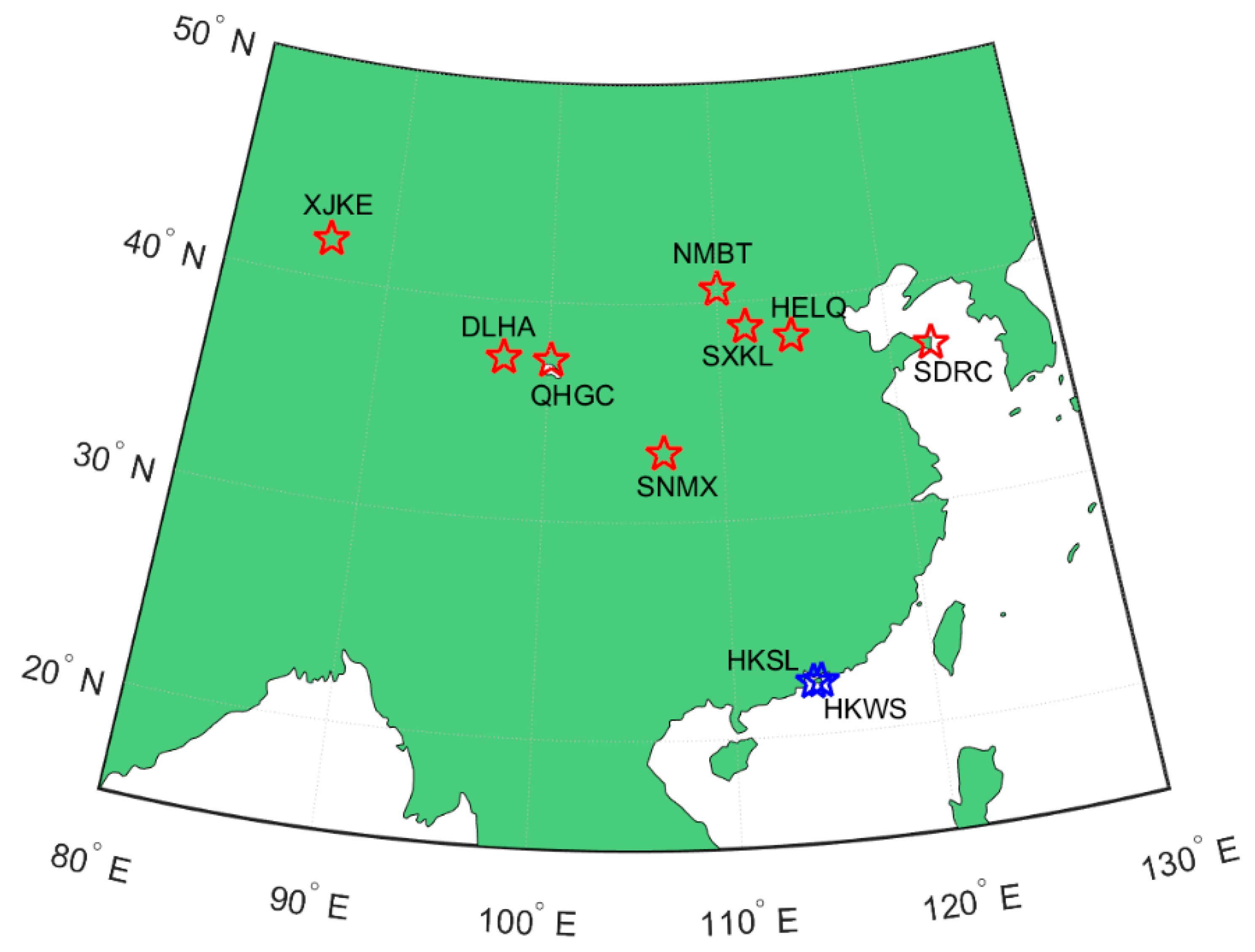
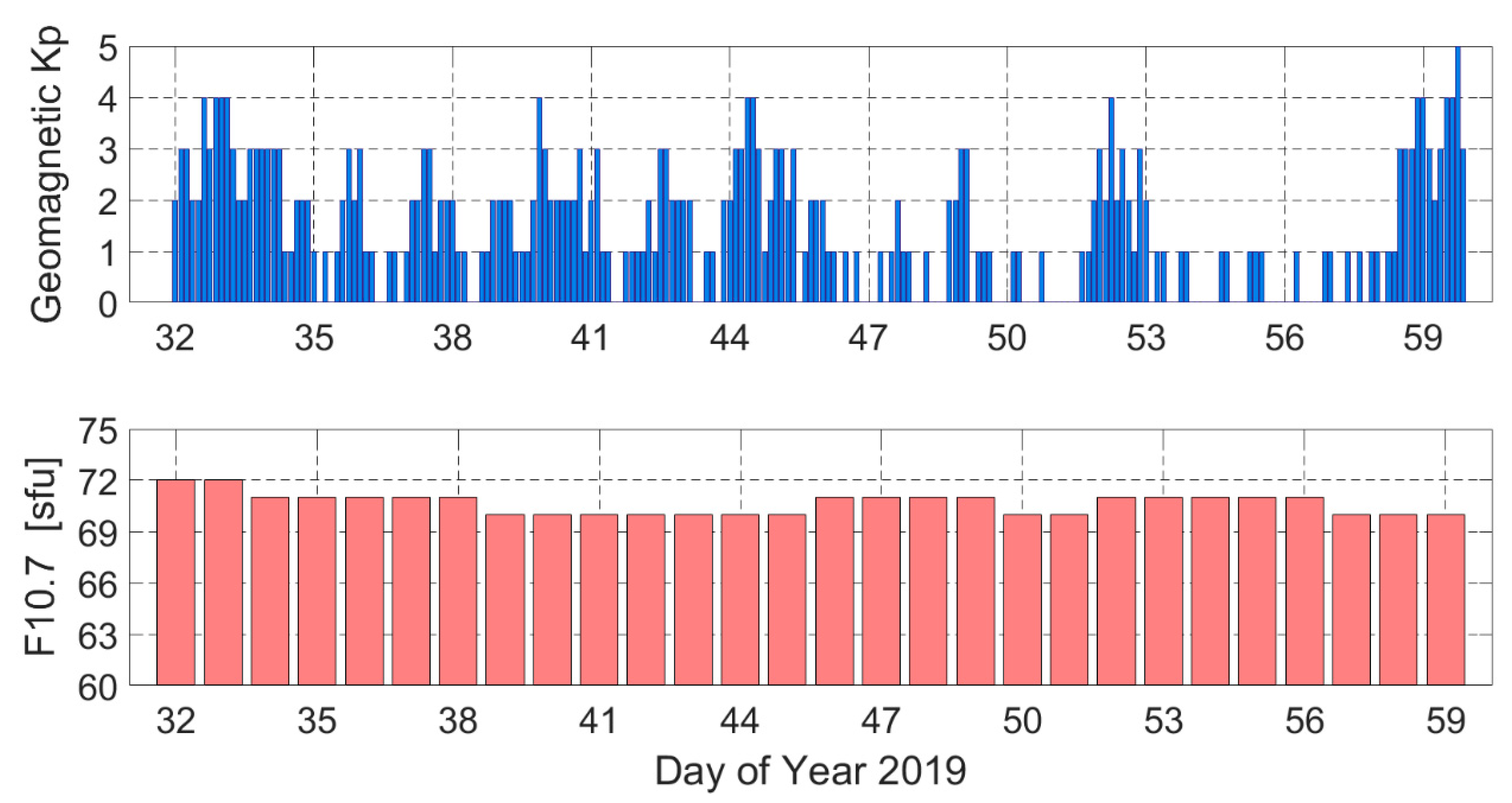
4. Experimental Data and Processing Strategy

To evaluate the effect of abovementioned four types of ionospheric delay on the multi-GNSS SF-SPP/PPP performances, GPS, GLONASS and BDS observation datasets collected from 2 MGEX stations and eight Crustal Movement Observation Network of China (CMONOC) stations for 1–28 February 2019 (DoY from 32 to 59) are selected and utilized for statistical analysis. Figure 1 shows the geographical distribution of the selected stations. Two MGEX stations and all CMONOC stations are equipped with LEICA GR50 or Trimble NetR9 receivers. To reflect the solar activity and ionosphere variation during the test period, the radio flux index F10.7 and geomagnetic Kp index are presented in Figure 2, where the ionosphere changes are relatively calm as the F10.7 value is less than 72 sfu and the Kp index is no more than 3 during most of the testing period. The multi-GNSS satellite orbits and clock offsets are corrected by the broadcast ephemeris or the final precise orbit and clock offset products provided by Deutsches GeoForschungsZentrum (GFZ). For the GIM model, we choose the products provided by CODE in this study. It should be noted that the CODE GIM based on spherical harmonic function rather than on local basis functions. Details of the models and strategies related to data processing for multi-GNSS SF-SPP/PPP are shown in

Table 1. Adopted models and strategies for multi-GNSS single-frequency SPP/PPP.

Item	Models/Strategies
Data span	1–28 February 2019
Frequency selection	GPS: L1/L2; GLONASS: G1/G2; BDS: B1/B2
Estimator	SPP: Least squares; PPP: Kalman filter
Sampling rate	30s
Elevation cutoff angle	10°
Satellite orbit and clock	SPP: broadcast ephemeris PPP: fixed to GFZ final orbit and clock offset products
Satellite TGD	Correct using broadcast ephemeris for SPP
Satellite differential code bias (DCB)	Correct using MGEX DCB products for PPP
Receiver and Satellite antenna	GPS and GLONASS PCO (phase center offset)/PCV (phase center variation) corrected with igs14.atx, BDS PCO corrected with the value released by ESA and PCV is not considered
Tropospheric delay	Modified (GPT2w + SAAS + VMF [27,28]) for the dry part and estimated for wet part as random-walk noise process
Ionospheric delay	Corrected using different ionosphere model for SPP, estimated as random-walk noise process for PPP
Tidal effects	Consider solid tides, ocean loading and polar tides [29]
Relativistic effects	Corrected by model
Phase windup	Corrected by model
Weighing strategy	Elevation-dependent weighing (1 for $E>30°$ otherwise $2\cdot \sin (E)$) is used
Station reference coordinates	IGS SINEX solutions
Station coordinates	SPP: estimated as white noises PPP: estimated as constants
Receiver clock	Estimated as white noise process
Receiver ISB	Set up for GLONASS/BDS and estimated as random-walk noise process [17]
GLONASS code IFB	Estimated for each GLONASS frequency
Phase ambiguities	Estimated as float constants for each arc

. The priori precision of GPS and GLONASS phase observation is set to 0.003 m. For the code observation, the priori precision of GPS is set to 0.3 m, while for GLONASS, is set to 0.6 m because of its higher code noise level [21]. Since the accuracy of BDS satellite orbits and clocks is worse than GPS, especially for geostationary earth orbit (GEO) satellites, this code observation also needs to be down-weighted [21,26]. The priori precision of BDS code observation is set to 0.6 m for inclined geosynchronous orbit (IGSO) and medium earth orbit (MEO) satellites, while the code observation precision of GEO satellites is set to 1.2 m. Besides, the BDS IGSO and MEO phase observation precision is set to 0.005 m, whereas the phase observation precision of BDS GEO satellites is set to 0.01 m. In order to maintain the consistency of the pseudo-range and carrier phase observations of the multi-GNSS constellation, b1 and b2 are used to denote observations on the first and the second frequency in this study, respectively.

In the ionosphere-constrained SF-PPP strategy, the setting of the weight of virtual ionospheric constrains will directly affect the positioning accuracy and convergence time. Generally, the priori variance of the ionospheric delay should be determined by the accuracy of the ionospheric model corrections. For the GPS-Klo and BDS-Klo based on Klobuchar model, their ionospheric priori variance is set to the square of the corresponding ionospheric correction value since these two models can correct about 50% of the ionospheric delay. For the BDS-Grid and GIM models, the ionospheric delay shows a strong spatial and temporal correlated, its variance can be defined as [16]:

$${\sigma }_{ion}^2=\frac{1}{m^2}\cdot \{\begin{array}{ll}{\sigma }_{ion,0}^2+{\sigma }_{ion,1}^2\cdot \cos (B)\cdot \cos (\frac{t-14}{12}\pi ),& 8<t<20\mathrm{or}B<\frac{\pi }{3}\\ {\sigma }_{ion,0}^2,& otherwise\end{array}$$

(17)

$$m=\sqrt{1-\frac{{\sin }^{2}Z}{(1+H_{ion}/R_{Earth})}}$$

(18)

where $m$ is the ionospheric mapping function. $Z$ is the zenith angle of the line of sight at a station. $H_{ion}$ is the height of the assumed ionosphere single layer, which is 450 km and 375 km for the GIM and Grid model, respectively. $R_{earth}$ is the average radius of the Earth in km. $B$ is the latitude of IPP. $t$ is the corresponding local time at IPP in hours. Since the precision of the GIM model is approximately 2–8 TECU, the variance of the zenith ionospheric delay ${\sigma }_{ion,0}^2$ and ${\sigma }_{ion,1}^2$ are set as 0.09 ${\mathrm{m}}^2$ and 0.09 ${\mathrm{m}}^2$, respectively [20]. Similarly, the Grid as a regional ionospheric model has an accuracy of 0.5 m in zenith direction, hence both ${\sigma }_{ion,0}^2$ and ${\sigma }_{ion,1}^2$ are set as 0.25 ${\mathrm{m}}^2$.

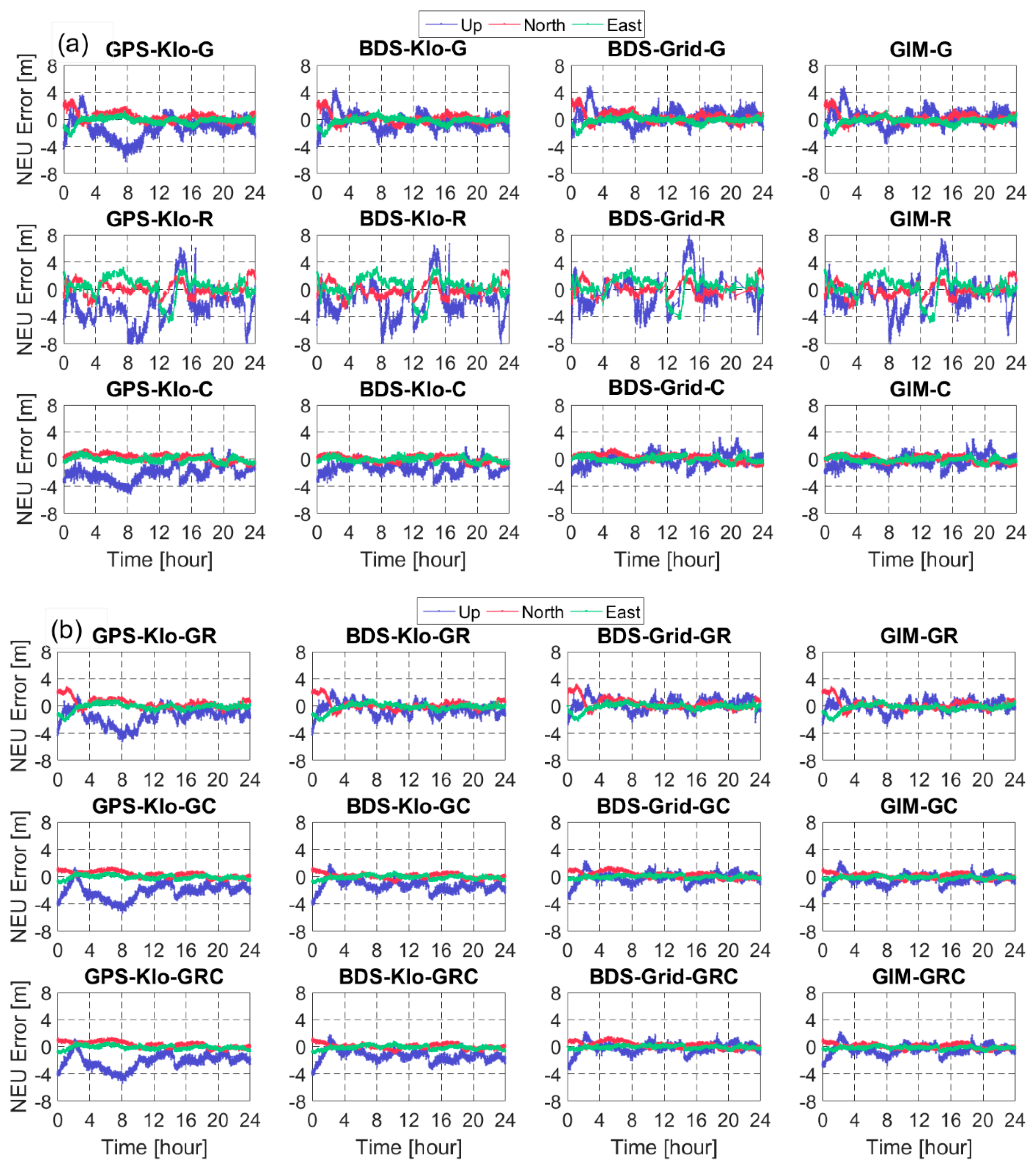
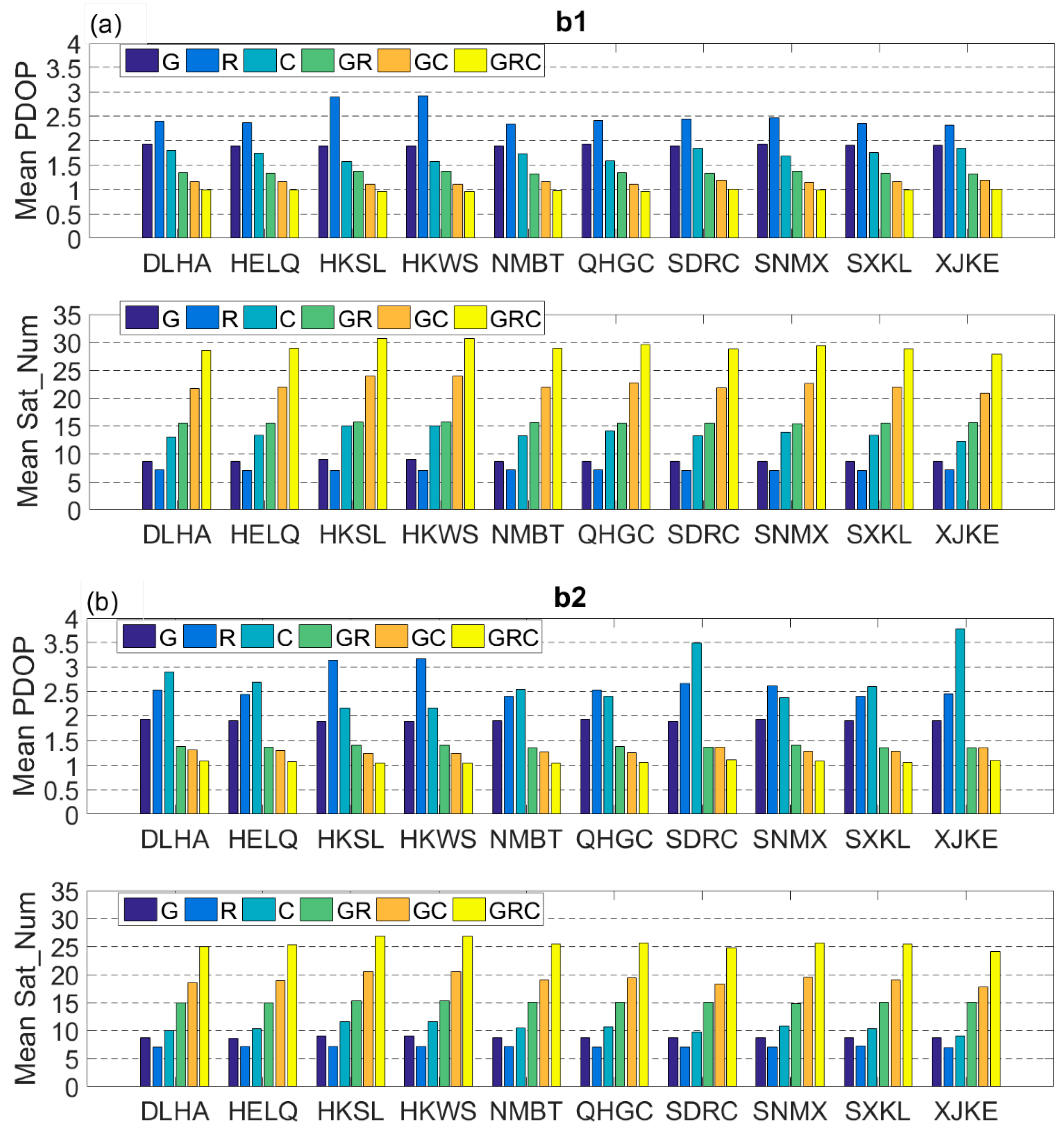
5. Performance of Single-Frequency SPP

The ionospheric delay is regarded as the largest error source in single-frequency positioning, and its model precision can be indirectly reflected by the accuracy of SF-SPP. Figure 3 presents the b1-based positioning errors of the station SNMX on 5 February 2019 for the north (N), east (E) and up (U) component based on the ionospheric delay correction of GPS-Klo, BDS-Klo, BDS-Grid and GIM. In general, the vertical error of SF-SPP with different schemes is relatively larger than the horizontal positioning error. It is obvious that the GPS + GLONASS + BDS SF-SPP can improve positioning accuracy because of the improved satellite geometry. The SF-SPP with GIM correction performs the best accuracy among all solutions, especially in the U direction. Although both GPS-Klo and BDS-Klo are based on the Klobuchar model, the positioning accuracy of SF-SPP with BDS-Klo correction is better than that of GPS-Klo, especially in the U component and during local time (LT) 21:00 to 5:00 (corresponding to UT 4:00 to 12:00). One reason is that the parameters of GPS-Klo are computed from an empirical model whereas the BDS-Klo coefficients are generated by processing real observation data from regional monitoring network and its accuracy is higher. Another point is that BDS-Klo parameters are updated every 2 h, more frequently than GPS-Klo, which will be conducive to accurately describe the ionospheric properties.

Figure 4 shows the mean number of visible satellites and mean Position Dilution of Precision (PDOP) in single- or multi-system SF-SPP at 10 selected stations on 5 February 2019. In test region, the average satellite number of BDS is larger than that of GPS. The number of GLONASS visible satellites is the least and the corresponding mean PDOP exceeds 2.4 for b1- or b2-based SPP. By the combination of multi-constellation, the mean PDOP decrease significantly and is no more than 1.5.

Table 2. RMS of SF-SPP with GPS-Klo, BDS-Klo, BDS-Grid and GIM based ionospheric correction for Figure 1 and b2 (unit: m).

System	Iono-Corr	b1				b2
		N	E	U	3D	N	E	U	3D
G	GPS-Klo	0.883	0.512	2.347	2.583	1.200	0.606	3.437	3.750
G	BDS-Klo	0.770	0.474	1.508	1.762	1.016	0.546	2.090	2.398
G	BDS-Grid	0.732	0.506	1.384	1.645	0.839	0.583	1.647	1.942
G	GIM	0.684	0.456	1.246	1.493	0.835	0.494	1.469	1.764
R	GPS-Klo	1.358	1.705	3.604	4.224	1.689	1.758	4.626	5.258
R	BDS-Klo	1.288	1.694	3.213	3.856	1.611	1.736	4.051	4.698
R	BDS-Grid	1.312	1.701	3.019	3.705	1.547	1.733	3.659	4.340
R	GIM	1.164	1.681	2.875	3.529	1.336	1.735	3.273	3.940
C	GPS-Klo	0.777	0.519	2.007	2.245	1.191	0.664	3.436	3.721
C	BDS-Klo	0.669	0.490	1.422	1.654	1.007	0.632	2.383	2.670
C	BDS-Grid	0.628	0.499	1.261	1.496	0.912	0.591	1.739	2.054
C	GIM	0.593	0.473	1.110	1.347	0.892	0.589	1.672	1.986
GR	GPS-Klo	0.855	0.510	2.263	2.499	1.172	0.601	3.269	3.577
GR	BDS-Klo	0.738	0.469	1.453	1.701	0.998	0.536	2.024	2.333
GR	BDS-Grid	0.694	0.505	1.364	1.612	0.786	0.575	1.559	1.841
GR	GIM	0.633	0.451	1.171	1.407	0.787	0.487	1.424	1.704
GC	GPS-Klo	0.724	0.420	1.989	2.201	1.094	0.540	3.077	3.376
GC	BDS-Klo	0.601	0.370	1.368	1.551	0.891	0.482	1.576	1.887
GC	BDS-Grid	0.515	0.379	0.907	1.111	0.694	0.457	1.343	1.581
GC	GIM	0.495	0.349	0.788	0.998	0.706	0.426	1.185	1.455
GRC	GPS-Klo	0.718	0.419	1.952	2.165	1.080	0.541	2.907	3.215
GRC	BDS-Klo	0.597	0.367	1.333	1.516	0.864	0.471	1.496	1.803
GRC	BDS-Grid	0.494	0.370	0.873	1.070	0.671	0.447	1.293	1.525
GRC	GIM	0.490	0.347	0.781	0.989	0.701	0.423	1.176	1.443

summarizes the RMS statistics in the N, E and U coordinate components, as well as RMS for the three-dimensional (3D) positioning error in different schemes on all days of all the test stations. From the figures and statistics, we can see that the positioning accuracy of GPS + GLONASS + BDS SF-SPP with GIM correction has the best performance. The reason is due to the fact that the GIM has the highest model accuracy as a post-processed product contrary to other ionospheric models, and the satellite geometry is the best with the increased number of visible satellites. For all the single-system SF-SPP solutions, the performance of GLONASS-only is the worst, which is caused by the higher PDOP and the worse accuracy of broadcast satellite orbits and clocks. With the development of the third-generation BDS (BDS-3), more BDS-3 satellites have been launched since 2017 and BDS has begun to provide a global PNT service at the end of 2018. In this study, the 10 selected stations during the test period can only receive the B1 and B3 observation signals of BDS-3 satellites, therefore the BDS b2 visible satellites number is generally the same as GPS, while the number of visible satellites in b1 is 3–6 more than GPS in the Asia-Pacific region. This is the reason that the BDS-only b1-based SF-PPP achieves better positioning performance than GPS. However, BDS b2 PDOP is larger than GPS and the accuracy of BDS GEO satellite orbits and clocks is comparatively lower, which result in the worse positioning accuracy of the b2-based BDS-only SPP. Compared with the GPS-Klo correction, the 3D positioning accuracy of GPS b1-based SPP with BDS-Klo, BDS-Grid and GIM corrections is improved by 31.8%, 36.3% and 42.2%, respectively. For GPS b2-based SPP, the improvement of 3D positioning accuracy for BDS-Klo, BDS-Grid and GIM models is 37.9%, 49.7% and 54.3%, respectively. In terms of GLONASS, compared with the GPS-Klo model, the improvements of the 3D positioning accuracy using BDS-Klo, BDS-Grid and GIM models is less than 25% for b1- or b2-based SPP. In general, for SF-SPP solutions, the GIM correction shows the best accuracy, and the positioning accuracy of the BDS-Klo and BDS-Gird model performs better than that of the GPS-Klo in all coordinate components, especially in the N and U direction. The multi-GNSS combined SF-SPP performance is better than the single-system solution.

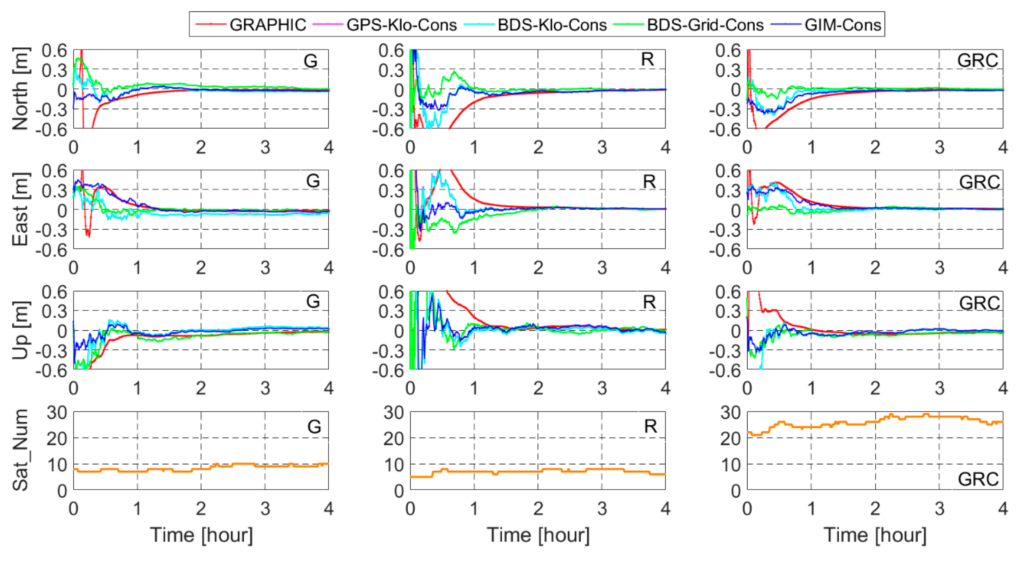
6. Performance of Single-Frequency PPP

The ionosphere-constrained PPP approaches are affected by the priori ionosphere information of different models. In this study, five different processing scenarios including GRAPHIC approach, GPS-Klo-, BDS-Klo-, BDS-Grid- and GIM-constrained approaches were applied in single- and multi-constellation SF-PPP. Figure 5 shows the SF-PPP positioning errors based on the different approaches for GPS, GLONASS and GPS + GLONASS + BDS solutions at QHGC station on 4 February 2019. It is obvious that the GRAPHIC approach needs a longer convergence time than other ionosphere-constrained approaches in single- and multi-constellation SF-PPP. The convergence time of the GIM-constrained SF-PPP in the N, E and U components are the shortest for all stations. It should be noted that the GPS-Klo- and BDS-Klo-constrained approaches have basically the same convergence time among different schemes since the two models are based on the Klobuchar model and have similar correction accuracy. Besides, with the integration of GPS, GLONASS and BDS, the improvement of PDOP with more GNSS satellite, contributes a significantly better convergence performance than a single constellation.

In order to compare the convergence performance of the abovementioned SF-PPP approach, in this study, the position filter is considered as converged when the positioning errors in the horizontal component is better than 0.3 m and keep within 0.3 m. Since the vertical positioning errors are relatively larger than the horizontal component, its criterion is set to 0.5 m. the convergence time is the period from the first epoch to the converged epoch. Figure 6 shows the average convergence time of b1 and b2 SF-PPP with different schemes for one month at all test stations.

Table 3. RMS of SF-PPP with the GRAPHIC approach, GPS-Klo-, BDS-Klo-, BDS-Grid-, and GIM-constrained approaches (unit: cm).

System	Iono-Corr	b1				b2
		N	E	U	3D	N	E	U	3D
G	GRAPHIC	1.43	3.06	5.01	6.09	1.56	3.04	9.13	9.91
G	GPS-Klo-Cons	2.12	4.12	5.14	6.98	2.30	4.90	9.99	11.54
G	BDS-Klo-Cons	2.14	3.58	5.18	6.70	2.37	4.40	10.29	11.67
G	BDS-Grid-Cons	2.43	3.36	5.01	6.58	2.25	4.00	8.80	10.15
G	GIM-Cons	2.24	3.34	4.88	6.38	2.34	3.59	9.10	10.31
R	GRAPHIC	1.80	3.64	5.92	7.19	1.91	3.86	8.59	9.62
R	GPS-Klo-Cons	2.44	4.58	7.14	8.89	2.38	5.20	10.31	11.86
R	BDS-Klo-Cons	2.38	4.14	7.34	8.80	2.38	4.76	10.52	11.81
R	BDS-Grid-Cons	2.49	4.12	6.62	8.18	2.56	4.69	8.86	10.45
R	GIM-Cons	2.34	4.09	6.44	8.05	2.29	3.85	9.23	10.43
C	GRAPHIC	5.83	8.20	18.29	20.92	5.59	7.20	15.47	18.04
C	GPS-Klo-Cons	6.80	9.33	19.52	22.77	5.67	8.52	15.31	18.82
C	BDS-Klo-Cons	6.84	8.88	19.88	22.90	5.37	7.04	15.56	18.31
C	BDS-Grid-Cons	7.08	9.31	18.07	21.58	5.90	8.18	15.33	18.52
C	GIM-Cons	6.47	8.66	17.61	20.96	5.37	7.43	14.61	17.65
GR	GRAPHIC	1.40	2.46	4.85	5.66	1.27	2.47	8.56	9.14
GR	GPS-Klo-Cons	1.87	3.64	5.15	6.66	1.89	4.35	9.97	11.14
GR	BDS-Klo-Cons	1.85	3.15	5.27	6.47	1.98	4.15	10.28	11.49
GR	BDS-Grid-Cons	1.89	2.88	4.79	5.96	2.02	3.37	8.73	9.76
GR	GIM-Cons	1.83	3.01	4.63	5.91	1.89	3.13	8.94	9.86
GC	GRAPHIC	1.44	3.04	4.92	6.01	1.55	3.03	9.00	9.78
GC	GPS-Klo-Cons	2.08	4.10	5.14	6.95	2.27	5.02	9.66	11.36
GC	BDS-Klo-Cons	2.10	3.70	5.19	6.76	2.22	4.48	10.16	11.52
GC	BDS-Grid-Cons	2.40	3.45	5.05	6.65	2.41	4.28	8.81	10.35
GC	GIM-Cons	2.16	3.34	4.89	6.35	2.33	3.48	9.10	10.27
GRC	GRAPHIC	1.42	2.43	4.84	5.65	1.40	2.40	8.55	9.11
GRC	GPS-Klo-Cons	1.89	3.83	5.01	6.62	1.96	4.29	10.06	11.28
GRC	BDS-Klo-Cons	1.97	3.16	5.12	6.38	2.00	3.96	10.37	11.45
GRC	BDS-Grid-Cons	2.02	2.98	4.99	6.21	2.15	3.50	8.43	9.58
GRC	GIM-Cons	1.95	2.91	4.64	5.90	2.11	3.27	8.77	9.79

summarizes the RMS positioning errors of SF-PPP with different schemes in the N, E, U and 3D components, the statistical result is calculated from the convergence epoch to the last epoch of a day. Among all the solutions, the BDS-only positioning performance is the worst, its positioning accuracy clearly performs worse than other single systems and the average convergence time is over 100 min. One reason is that the accuracy of BDS precise orbit and clock is lower than other systems, the other point is that BDS PCV correction is currently unavailable. For GLONASS-only SF-PPP, its positioning accuracy slightly performs worse than GPS-only solutions. However, the convergence time of the GLONASS SF-PPP with different approaches clearly performs worse than GPS-only solutions. The improvements of four types of ionosphere-constrained GLONASS-only solutions are very close and are no more than 15% compared with the GRAPHIC approach. The main reason is that the partial ionospheric delay errors are absorbed by IFBs parameter due to the strong correlation between the satellite-specific IFBs and slant ionospheric delays [30]. In the GRAPHIC approach, the average convergence time of the GPS + GLONASS + BDS solution can be reduced by up to 32% compared with the GPS-only SF-PPP, which is mainly due to the optimization of satellite geometry. By introducing the priori ionosphere information, the improvement in average convergence time of GPS-Klo-, BDS-Klo-, BDS-Grid- and GIM-constrained GPS + GLONASS + BDS b1 SF-PPP is 11.2%, 11.9%, 21.3% and 39.6%, respectively, compared with the GRAPHIC approach. As for the ionosphere-constrained b2 SF-PPP, similar performance in convergence time is achieved as in b1 SF-PPP solutions. On the other hand, the positioning accuracy of the GPS + GLONASS + BDS b1 SF-PPP can reach 1–3 cm in the horizontal component and 4–5 cm in the vertical component. The RMS 3D positioning errors of the BDS-Grid- and GIM-constrained SF-PPP is basically the same and is no more than 1 cm larger than that of the GRAPHIC approach, while the GPS-Klo- and BDS-Klo-constrained solutions can be up to 2 cm. The lower accuracy of the two ionospheric models is an important factor. In summary, the GIM-constrained SF-PPP has the best positioning accuracy and shortest convergence time in the different ionosphere-constrained SF-PPP schemes. The performance of BDS-Grid-constrained solution is much better than that of GPS-Klo or BDS-Klo, especially for the convergence, which exhibits agreement with the accuracy of selected ionospheric models.

7. Conclusions

In this study, we evaluated the different ionospheric models including GPS-Klo, BDS-Klo, BDS-Grid and GIM effects on multi-GNSS single-frequency SPP and PPP performances. One month of data collected in 2019 at 10 stations was processed with different positioning scenarios. During the test period, the solar remained calm and the ionosphere was quiet. Comprehensive statistical analyses indicated that the performance of SF-SPP with GIM correction shows the best, and the RMS positioning errors of SF-SPP based on the regional ionospheric model BDS-Klo and BDS-Grid is much better than the solution with the GPS-Klo model in the N and U components. Although both GPS-Klo and BDS-Klo are based on the Klobuchar model, the BDS-Klo correction accuracy at night is clearly better than the GPS-Klo model.

By introducing the priori ionosphere information, the average convergence time of the SF-PPP is reduced. Compared with the GRAPHIC approach, the improvement in the b1 SF-PPP convergence time of the GPS-Klo-, BDS-Klo-, BDS-Grid- and GIM-constrained GPS + GLONASS + BDS solutions is 11.2%, 11.9%, 21.3% and 39.6%, respectively. Due to the strong correlation between the IFBs and ionospheric delays, the improvement of convergence time for GLONASS-only SF-PPP with the different ionosphere-constrained was very close and no more than 15%. The positioning accuracy of the BDS-Grid- and GIM-constrained SF-PPP was basically the same as the GRPAHIC approach, whereas the GPS-Klo- and BDS-Klo-constrained approaches were slightly worse due to the relatively lower accuracy of the two ionospheric models. In summary, through the combination of GPS, GLONASS and BDS, the positioning accuracy and convergence performance of all SF-SPP/PPP schemes can be significantly improved.

References

1. Zumberge, J.F.; Heflin, M.B.; Jefferson, D.C.; Watkins, M.M.; Webb, F.H. Precise point positioning for the efficient and robust analysis of GPS data from large network. J. Geophys. Res. 1997, 102, 5005–5017. [Google Scholar] [CrossRef]
2. Kouba, J.; Heroux, P. Precise point positioning using IGS orbit and clock products. GPS Solut. 2001, 5, 12–28. [Google Scholar] [CrossRef]
3. Ovstedal, O. Absolute positioning with single-frequency GPS receivers. GPS Solut. 2002, 5, 33–44. [Google Scholar] [CrossRef]
4. Cai, C.; Liu, Z.; Luo, X. Single-frequency ionosphere-free precise point positioning using combined GPS and GLONASS observations. J. Navig. 2013, 66, 417–434. [Google Scholar] [CrossRef]
5. Sterle, O.; Stopar, B.; Preseren, P.P. Single-frequency precise point positioning: An analytical approach. J. Geod. 2015, 89, 793–810. [Google Scholar] [CrossRef]
6. Liu, Z.; Yang, Z. Anomalies in broadcast ionospheric coefficients recorded by GPS receivers over the past two solar cycles (1992–2013). GPS Solut. 2016, 20, 23–37. [Google Scholar] [CrossRef]
7. Klobuchar, J.A. Ionospheric time-delay algorithm for single-frequency GPS users. IEEE Trans. Aerosp. Electron. Syst. 1987, 23, 325–331. [Google Scholar] [CrossRef]
8. Schaer, S. Mapping and Predicting the Earth’s Ionosphere Using the Global Positioning System. Ph.D. Thesis, University of Bern, Bern, Switzerland, 1999. [Google Scholar]
9. Le, A.Q.; Tiberius, C. Single-frequency precise point positioning with optimal filtering. GPS Solut. 2007, 11, 61–69. [Google Scholar] [CrossRef]
10. Wu, X.; Hu, X.; Wang, G.; Zhong, H.; Tang, C. Evaluation of COMPASS ionospheric model in GNSS positioning. Adv. Space Res. 2013, 51, 959–968. [Google Scholar] [CrossRef]
11. Wu, X.; Zhou, J.; Tang, B.; Cao, Y.; Fan, J. Evaluation of COMPASS ionospheric grid. GPS Solut. 2014, 18, 639–649. [Google Scholar] [CrossRef]
12. Radicella, S.M. The NeQuick model genesis, uses and evolution. Ann. Geophys. 2009, 52, 417–422. [Google Scholar]
13. Choy, S.; Silcock, D. Single-frequency ionosphere-free precise point positioning: A cross-correlation problem? J. Geod. Sci. 2011, 1, 314–323. [Google Scholar] [CrossRef]
14. Shi, C.; Gu, S.; Lou, Y.; Ge, M. An improved approach to model ionospheric delays for single-frequency precise point positioning. Adv. Space Res. 2012, 49, 1698–1708. [Google Scholar] [CrossRef]
15. Montenbruck, O. Kinematic GPS positioning of LEO satellites using ionosphere-free single-frequency measurements. Aerosp. Sci. Technol. 2003, 7, 396–405. [Google Scholar] [CrossRef]
16. Zhang, H.; Gao, Z.; Ge, M.; Niu, X.; Huang, L.; Tu, R.; Li, X. On the convergence of ionospheric constrained precise point positioning (IC-PPP) based on undifferential uncombined raw GNSS observations. Sensors 2013, 13, 15708–15725. [Google Scholar] [CrossRef]
17. Zhou, F.; Dong, D.; Li, P.; Li, X.; Schuh, H. Influence of stochastic modeling for inter-system biases on multi-GNSS undifferenced and uncombined precise point positioning. GPS Solut. 2019, 23, 59. [Google Scholar] [CrossRef]
18. Shi, C.; Yi, W.; Song, W.; Lou, Y.; Yao, Y.; Zhang, R. GLONASS pseudorange inter-channel biases and their effects on combined GPS/GLONASS precise point positioning. GPS Solut. 2013, 17, 439–451. [Google Scholar]
19. Zhou, F.; Dong, D.; Ge, M.; Li, P.; Wickert, J.; Schuh, H. Simultaneous estimation of GLONASS pseudorange inter-frequency biases in precise point positioning using undifferenced and uncombined observations. GPS Solut. 2018, 22, 19. [Google Scholar] [CrossRef]
20. Su, K.; Jin, S.; Hoque, M.M. Evaluation of ionospheric delay effects on multi-GNSS positioning performance. Remote Sens. 2019, 11, 171. [Google Scholar] [CrossRef]
21. Pan, L.; Zhang, X.; Liu, J.; Li, X.; Li, X. Performance evaluation of single-frequency precise point positioning with GPS, GLONASS, BeiDou and Galileo. J. Navig. 2017, 70, 465–482. [Google Scholar] [CrossRef]
22. Jakowski, N.; Hoque, M.M.; Mayer, C. A new global TEC model for estimating transionospheric radio wave propagation errors. J. Geod. 2011, 85, 965–974. [Google Scholar] [CrossRef]
23. Hoque, M.M.; Jakowski, N. An alternative ionospheric correction model for global navigation satellite systems. J. Geod. 2015, 89, 391–406. [Google Scholar] [CrossRef]
24. CSNO. BeiDou Navigation Satellite System Signal in Space Interface Control Document—Open Service Signal B3I (Version 1.0); China Satellite Navigation Office: Beijing, China, 2018.
25. Schaer, S.; Gartner, W.; Feltens, J. IONEX: The ionosphere map exchange format vision 1. In Proceedings of the IGS AC Workshop, Darmstadt, Germany, 9–11 February 1998. [Google Scholar]
26. Montenbruck, O.; Steigenberger, P.; Hauschild, A. Multi-GNSS signal-in-space range error assessment—Methology and results. Adv. Space Res. 2018, 61, 3020–3038. [Google Scholar] [CrossRef]
27. Boehm, J.; Werl, B.; Schuh, H. Troposphere mapping functions for GPS and very long baseline interferometry from European Centre for Medium-Range Weather Forecasts operational analysis data. J. Geophys. Res. 2006, 111, B02406. [Google Scholar] [CrossRef]
28. Boehm, J.; Moller, G.; Schindelegger, M.; Pain, G.; Weber, R. Development of an improved empirical model for slant delays in the troposphere (GPT2w). GPS Solut. 2015, 19, 433–441. [Google Scholar] [CrossRef]
29. Gérard, P.; Luzum, B. IERS Conventions; IERS Technical 2010 Note 36; Verlag des Bundesamts für Kartographie und Geodäsie: Frankfurt am Main, Germany, 2010. [Google Scholar]
30. Schonemann, E.S.; Becker, M.; Springer, T. A new approach for GNSS analysis in a multi-GNSS and multi-signal environment. J. Geod. Sci. 2011, 1, 204–214. [Google Scholar] [CrossRef]
Figure 1. Geographical distribution of the selective MGEX (blue) and CMONOC (red) stations.
Remotesensing 11 02070 g001
Figure 2. Geomagnetic Kp index and F10.7 values on 1–28 February 2019.
Remotesensing 11 02070 g002
Figure 3. Positioning errors of b1 SF-SPP with different ionospheric models (GPS-Klo, BDS-Klo, BDS-Grid and GIM) in (a) single-system or (b) multi-system at SNMX station (DoY 36 in 2019, sum of Kp = 0.88, F10.7 = 71 sfu). Where, e.g., GPS-Klo-GRC represents the SF-SPP results using data of GPS + GLONASS + BDS with ionosphere delay corrected using the GPS-Klo model, and the abbreviation G, R and C represent GPS, GLONASS and BDS, respectively.
Remotesensing 11 02070 g003
Figure 4. Mean number of satellites and mean PDOP for different SF-SPP processing scenarios at 10 selected stations on 5 February 2019, (a) b1 SPP; (b) b2 SPP; the abbreviation G, R and C represent GPS, GLONASS and BDS, respectively.
Remotesensing 11 02070 g004
Figure 5. Comparison of positioning error of b1 SF-PPP with different schemes for GPS, GLONASS and GPS + GLONASS + BDS solutions at QHGC station (DoY 35 in 2019, sum of Kp = 1.25, F10.7 = 71 sfu). The corresponding satellite numbers are represented by the yellow curve. The abbreviation “Cons” represents “Constrained”.
Remotesensing 11 02070 g005
Figure 6. Average convergence time of SF-PPP with different schemes for GPS-only, GLONASS-only, BDS-only, GPS + GLONASS, GPS + BDS and GPS + GLONASS + BDS solutions using datasets at 10 stations over one month.
Remotesensing 11 02070 g006