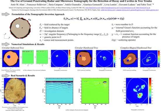
The Use of Ground Penetrating Radar and Microwave Tomography for the Detection of Decay and Cavities in Tree Trunks

Abstract

Aggressive fungal and insect attacks have reached an alarming level, threatening a variety of tree species, such as ash and oak trees, in the United Kingdom and beyond. In this context, Ground Penetrating Radar (GPR) has proven to be an effective non-invasive tool, capable of generating information about the inner structure of tree trunks in terms of existence, location, and geometry of defects. Nevertheless, it had been observed that the currently available and known GPR-related processing and data interpretation methods and tools are able to provide only limited information regarding the existence of defects and anomalies within the tree inner structure. In this study, we present a microwave tomographic approach for improved GPR data processing with the aim of detecting and characterising the geometry of decay and cavities in trees. The microwave tomographic approach is able to pinpoint explicitly the position of the measurement points on the tree surface and thus to consider the actual geometry of the sections beyond the classical (circular) ones. The robustness of the microwave tomographic approach with respect to noise and data uncertainty is tackled by exploiting a regularised scheme in the inversion process based on the Truncated Singular Value Decomposition (TSVD). A demonstration of the potential of the microwave tomography approach is provided for both simulated data and measurements collected in controlled conditions. First, the performance analysis was carried out by processing simulated data achieved by means of a Finite-Difference Time-Domain (FDTD) in three scenarios characterised by different geometric trunk shapes, internal trunk configurations and target dimensions. Finally, the method was validated on a real trunk by proving the viability of the proposed approach in identifying the position of cavities and decay in tree trunks.

1. Introduction

Swift and effective tree health monitoring and assessment is crucial for the protection of ecosystems and the maintenance of sustainable climate conditions [1]. Tree diseases play an important role in regulating the development of forests [2], and their existence is, therefore, necessary to maintain the natural balance. However, human activities have often contributed to alter this balance, dismantling rather frequently the protective geographical barriers of ecosystems and affecting wildlife habitats [3,4]. As a result of anthropic activities, such as human population increases [5], international travel [4], global plant trade [6] and timber trade [7], exotic pathogens and fungi have infested entire regions. Furthermore, the rise in global temperatures due to ongoing climate change contributes to the rapid spread of these epidemics [4,8]. At the present, entire ecosystems are endangered by a number of these infections, which are known as emerging infectious diseases (EIDs) [9,10]. The consequence of a spread of EIDs is now dramatic, as these infections are on the rise [11] and can result in the complete extinction of certain tree species [12].

Some of the most significant examples of EIDs are represented by ash dieback, acute oak decline (AOD) and Dutch elm disease (DED) [13,14,15]. The first cases of ash dieback in Europe were reported in 1992, and its spread to the United Kingdom dates back to 2012 [16]. Given that most species of ash trees are unable to withstand this disease, the infection has spread extremely rapidly, and predictions foresee that most of these trees will die within the next twenty years [17]. The AOD, the incidence of which has dramatically increased in the UK over the last ten years [14], is also particularly aggressive, as it can cause the death of the infected tree within a few years [18]. DED is considered one of the most dangerous tree diseases in the world. The fungus causing this disease spreads via a particular species of bark beetles, and attacks the foliage and the tips of the branches, resulting in the death of the tree, which becomes starved of nutrients. DED has been endemic to the UK since the 1920s, but a severe new epidemic began in the 1970s, apparently being imported from North America [19,20].

According to the international scientific community, the control and elimination of EIDs is a complex but necessary task. Novel multidisciplinary approaches are encouraged for diagnosing, monitoring and controlling the spread of EIDs [10]. Within this framework, it is important to emphasise that an early-stage diagnosis of the diseases is crucial to provide remedial actions. The most significant obstacle to achieving this goal is that the first symptoms of decay are often located in the inner core of the tree, so there are no visible signs of disease on the outer surface of the tree [21].

In view of the above, decay detection in living trees is doubtless a challenging task. Simple methods based on the operator’s experience, such as assessing the presence of decay by sounding the tree (namely, striking the tree trunk with a hammer and listening to the sound it makes) are still widely used. Nonetheless, these methods are not very reliable, as they can only assess the presence of decayed wood, but no information can be gained on the stage that the decay has reached [22]. Presently, destructive methods such as the core-drilling technique [23] are still widely applied for the assessment of the internal structure of trees. However, the reliability of these techniques is offset by their invasive effects. Their implementation is time-consuming and laborious, as a large number of samples may be needed to assess the real conditions of the investigated tree. This also causes irreversible damage to the tree itself, exposing it to further contamination by pathogens or fungi [24,25]. Not least, destructive testing methods can only provide information about the tree at the time of sampling and at the survey points, and are therefore ineffective for the investigation of the developmental process of decay. In view of the above, destructive methods are increasingly recognised as being unsuitable for the assessment of living trees.

On the other hand, the use of non-destructive testing (NDT) methods in this application area is gaining popularity, in view of their versatility, efficiency and their ability to provide reliable results at an adequate cost. Above all, these methods provide accurate information about the inner structure of the investigated materials without causing any damage. This also allows non-destructive surveys to be planned and repeated on a routine basis, therefore enabling the long-term monitoring of the tree. Within this context, the use of NDT methods such as resistograph testing [26], electrical resistivity tomography (ERT) [27], ultrasound tomography [28], infrared thermography [29], X-ray tomography [30] and microwave tomography [31] has been reported in this application area.

Within the available NDT methods, Ground Penetrating Radar (GPR) is widely acknowledged to be a very effective non-destructive geophysical tool. GPR has been increasingly used in a wide range of disciplines such as archaeological investigations [32,33], the detection of landmines [34,35], tunnels [36,37], bridge deck analysis [38], civil and environmental engineering applications [39,40,41], and planetary exploration [42,43,44]. It is also broadly employed for soil characterisation [45,46] and the detection of buried objects [47,48,49].

Recently, several studies have been carried out on the feasibility of using GPR for large-scale investigations in forestry engineering as well as for the monitoring of tree trunks [50,51,52,53] and root systems [54,55,56,57]. In this regard, the numerical simulation of the GPR signal is relatively recent and it has proven to aid in the interpretation of radar images when assessing the geometric and physical characteristics of trunks and potential decay [52,58,59].

Nevertheless, the cylinder-like shape of tree trunks creates challenges with the use of traditional GPR data processing techniques, which are relatively straightforward to use on planar surfaces and interfaces (such as in the case of subsoil investigations). These conditions instead favour the use of tomographic approaches. Microwave imaging of cylindrical objects has been widely employed for biomedical applications [60], using inversion schemes primarily based on linear approximations of the scattering phenomenon [61,62]. Further application examples of these methods are found in other cylinder-like objects, such as columns [63] and tunnel imaging [37]. A similar approach has been put into practice for the evaluation of the internal structure of tree trunks, with encouraging results [31,58].

Tomographic approaches are relatively onerous from a computational point of view, and also require multiple measurements to be carried out with multiple separate transmitters and receivers, often using bespoke antenna systems [31]. Conversely, GPR surveys are commonly carried out using common-offset commercial antennas [64]; in this case, the simplicity of the measurement configuration is offset by a reduction in the quantity of information available for imaging tasks. For this reason, a signal processing approach that is capable of locating decay and of providing an indication of its dimensions using a common-offset commercial system would be a significant improvement to the assessment of living trees.

Within this framework, the application of microwave tomography using a common-offset commercial GPR system is presented in this paper. The main aim of this research is to provide a viable and robust data processing approach for the effective detection of decay and cavities in tree trunks using a common-offset commercial GPR system. To achieve this goal, the viability of using a tomographic inversion approach is assessed in the paper and a set of Finite-Difference Time-Domain (FDTD) simulations relevant to different trunk configurations and dimensions of the targets are carried out. Then, the method is validated on a real trunk.

The paper is organised as follows. Section 2 reports the theoretical background on the GPR technique and the use of the microwave tomographic inversion approach. Section 3 presents the methodology, sorted in terms of the numerical simulation and the real-life investigation stages, and the data processing framework. Section 4 reports and discusses the results. A conclusion and avenues for future research are presented in Section 5.

2. Theoretical Background

2.1. GPR Principles

GPR is a geophysical inspection technique usually employed for non-destructive subsurface investigations. The working principle of a GPR system is based upon the emission of pulsed electromagnetic (EM) waves towards the investigated domain. The EM wave propagates in the medium until it reaches an EM anomaly that gives rises to a scattered field that is collected by the receiving antenna(s). A GPR time-domain trace is characterised by a series of peaks, whose amplitude depends on three main factors: the nature of the reflector, the nature of the traversed medium, and the curve of the applied amplification [60,65]. Typically, three visualisation modes can be considered for a GPR signal, providing three different levels of information: (i) An A-scan, i.e., a single radar trace along the depth axis; (ii) a B-scan, i.e., a set of sequential single radar traces collected along a specific scanning direction; (iii) a C-scan, i.e., the volumetric representation achieved by superposing a set of B-scans [66].

A variety of information can be collected with GPR, such as the two-way travel time distance between reflection peaks at layer interfaces/target positions (e.g., rebars), and the amplitude and phase of the signal. Despite raw radargrams providing some visual information about the probed scene, their interpretation is very challenging in many practical cases (e.g., tree trunks) since only a distorted geometric representation of the targets can be obtained. To this end, focusing algorithms for GPR data are necessary to recover the geometrical characteristics of the targets. In the present work, a microwave tomographic approach is used to overcome the limitations of traditional GPR data processing techniques (e.g., migration) that relate to mostly planar interfaces [67,68,69].

2.2. Formulation of the Tomographic Inversion Approach

The microwave tomographic approach considered in this paper exploits a linearised model of the EM scattering based on the Born Approximation (BA) [67,69]. It is known that BA allows achieving a quantitative reconstruction only in the case of anomalies that are weak scatterers compared to the host medium. On the other hand, when the assumption of weak scattering is removed, solving an inverse scattering problem based on BA still allows reliable information to be gained about the presence, location and shape of potential targets [67,68,69].

A 2D scenario showing the cross-section of a tree trunk at a fixed height is considered in Figure 1. The investigation domain D corresponds to the trunk section with a constant relative dielectric permittivity ${\epsilon }_b$.

The scattering phenomenon is activated by a source modelled as a filamentary current polarised along the y-axis (TM polarisation) and radiating an electromagnetic signal. The exp(jωt) time dependence is assumed, with ω = 2πf being the angular frequency and f belonging to the frequency range $\left[f_{min},f_{max}\right].$ The source and the measurement points ${\mathit{r}}_m$, i.e., the location where the scattered field is collected, are located at the boundary of the probed area. Accordingly, the scattering model is defined under a multi-monostatic/multi-frequency measurement configuration. A generic point in D is denoted with $\mathit{r}$ and $\chi =\frac{\epsilon }{{\epsilon }_b}-1$ is the contrast function accounting for the presence of targets, which is modelled as a variation of the permittivity with respect to the known permittivity of the investigated medium.

For each measurement point ${\mathit{r}}_m$ and angular frequency ω, the scattering phenomenon under the BA is described by the linear integral equation (Equation (1)):

$$E_s\left({\mathit{r}}_m,\omega \right)=k_b^2{{\displaystyle \iint }}_D{g}_e\left({\mathit{r}}_m,\mathit{r},\omega \right)E_{inc}\left(\mathit{r},{\mathit{r}}_m,\omega \right)\chi \left(\mathit{r}\right)d\mathit{r}=L\left(\mathsf{\chi }\right)$$

(1)

where, $k_b^{}$ is the wave-number in D. Bold fonts are used in Equation (1) to denote vector quantities. Equation (1) expresses the field $E_s$ scattered by the target (measured data) as radiated by the equivalent “source” defined by the product between the unknown contrast function χ and the incident field $E_{inc}$ in D, which is the field in absence of targets. The quantity $g_e$ is the ‘external’ Green’s function that accounts for the field generated at ${\mathit{r}}_m$ by the elementary source located at $\mathit{r}$. The scattering model underlying the inversion model considered in this work is based on the assumption that the radar signal propagation occurs in a homogenous medium. Such an assumption allows to simplify considerably the computation of the scattering operator L as the Green’s function is available in closed form, i.e.,:

$$g_e\left({\mathit{r}}_m,\mathit{r},\omega \right)=\frac{j}{4}{H}_0^{\left(2\right)}\left(k_b\left|{\mathit{r}}_m-\mathit{r}\right|\right)$$

(2)

where $H_0^{\left(2\right)}$ is the Hankel function of second kind and zero order.

It is noteworthy to emphasise that, as far as a qualitative image of the scene has to be achieved and the GPR data are collected at the air–tree interface, the homogenous medium assumption provides quite reliable results with a relatively low computation effort. On the other hand, more complicated layered models could be in principle adopted, although this would require the use of a-priori information about the inner structure of the trunk, which is not available for the on-field surveys.

The kernel of the linear radiation operator $L$ is equal to the product between the external Green’s function $g_e$ and the incident field $E_{inc}$. The operator $L$ directly relates the unknown contrast function to the scattered field. Therefore, the reconstruction of the contrast function is carried out through the inversion of Equation (1), that is an ill-posed linear inverse problem [69]. Indeed, $L$ is a compact operator and this entails that a solution of the problem may not exist and does not depend continuously on the data, as deeply discussed in Bertero and Boccacci [70]. From a practical viewpoint, due to the inherent noise in the data, only a limited accuracy of representation of the scenario under investigation can be obtained. The lack of existence and stability of a solution can be remedied by introducing a regularisation scheme [70,71]. However, the necessity to regularise the inverse problem introduces the use of a spatial filtering of the retrievable components of the unknown [69,71].

The regularisation of the inverse problem is herein carried out by resorting to the Truncated Singular Value Decomposition (TSVD) tool. Following the discretisation of Equation (1), the imaging task amounts to solving the matrix inverse problem:

$$E_s=L\mathsf{\chi }$$

(3)

where $E_s$ is the K = M × F dimensional data vector, M being the number of spatial measurement points and F the number of frequencies, $\mathsf{\chi }$ is the N-p dimensional unknown vector, $N_p$ being the number of pixels in D, and L is the K × $N_p$ dimensional matrix obtained by discretising the integral operator in Equation (1). Since the matrix L stems from the discretisation of an ill-posed integral equation, the inversion of this matrix is an ill-conditioning problem, which means that the solution is very sensitive to measurement uncertainties and data noise. Hence, the TSVD scheme, as expressed in Equation (3), can be applied as a regularisation scheme in order to obtain a robust and physically meaningful solution:

$$\tilde{\mathit{\chi }}={\displaystyle \sum }_{n=1}^H\frac{\langle {\mathit{E}}_s,{\mathit{u}}_n\rangle }{{\sigma }_n}{\mathit{v}}_n$$

(4)

In Equation (4), 〈 , 〉 denotes the scalar product in the data space, H is a truncation index, ${\left\{{\sigma }_n\right\}}_{n=1}^Q$ is the set of singular values of the matrix L ordered in a decreasing way, ${\left\{{\mathit{u}}_n\right\}}_{n=1}^Q$ and ${\left\{{\mathit{v}}_n\right\}}_{n=1}^Q$ are the sets of the singular vectors in the data and the unknown spaces, respectively. The index H ≤ Q ($Q=\min \left\{K,N_p\right\}$) defines the “degree of regularisation” of the solution and is set in order to find a trade-off between the accuracy and the spatial resolution on one side (tending to increase H) and the solution stability on the other side (tending to reduce H).

The imaging result is a spatial map corresponding to the modulus of the retrieved contrast vector $\tilde{\mathit{\chi }}$ normalised to its maximum value in the scenario. Hence, the regions of D where the modulus of $\tilde{\mathit{\chi }}$ are significantly different from zero are representative of the position and geometry of the targets.

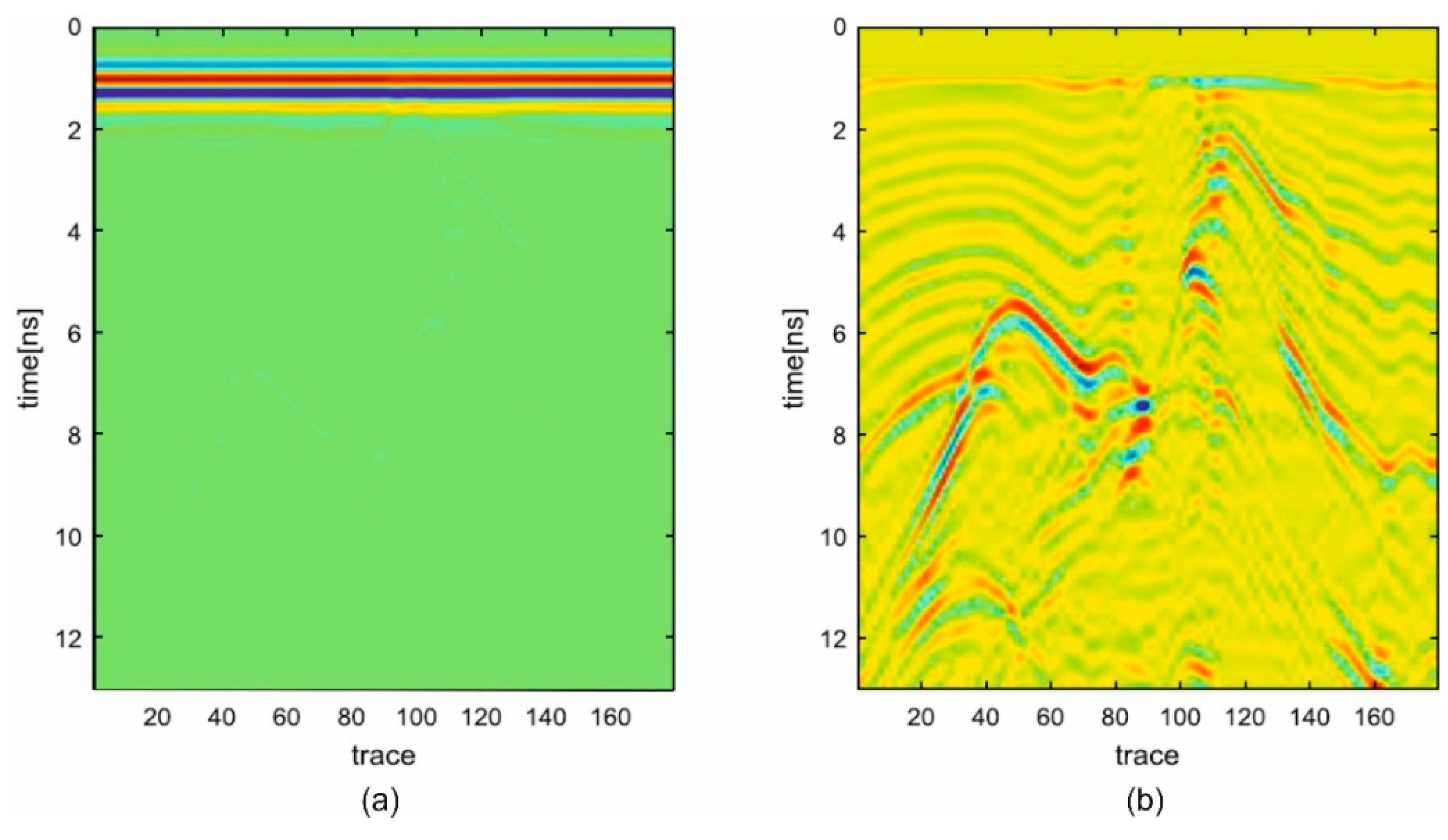
2.3. Data Pre-Processing

In relation to the results presented in this paper, the raw data were collected in the time domain, whereas the input data to the inverse scattering approach were given in the frequency domain. In view of this, a pre-processing stage was necessary in order to achieve the appropriate input data such that the inverse scattering approach could be applied. The pre-processing consists of the following operations:

Zero timing: This step consisted of cutting the first part of the signal, up to the flat-like reflection of the air–tree interface. Specifically, the zero time of the radargram was fixed in correspondence of the first peak of the radar signal, which was assumed as coincident with the location of the air–tree interface.

Time-gating: This procedure consisted of selecting the observation time window wherein the useful portion of the signal was expected to occur. Since the time of flight is related to the target depth, the time gating allowed analysis of only the portion of the radargram corresponding to the depth range of interest, which was fixed by the maximum radius of the tree cross-section. Note that the lower boundary of the time-gating window could be selected as larger than the time zero in order to perform a more severe filtering of the first strong reflections coming from the air–tree interface.

Background removal: This operation consisted of replacing every single A-scan of the radargram with the difference between the single A-scan value and the average value of all the A-scans in the radargram. The background removal eliminated all the flat interfaces in the data (including the air–tree interface, only partially removed by the application of the zero timing) and usually allowed provision of a cleaner image of the scene.

Linear gain versus time (depth): Deeper targets scatter a signal lower than shallower targets. In order to compensate this effect, a gain variable versus the depth distance is applied to the raw data.

Fourier transform: The time domain filtered raw data are converted into the frequency domain in order to be processed according to the microwave tomography approach. No window functions have been applied to the time domain pre-processed data before conversion into frequency domain data.

3. Methodology

3.1. Numerical Simulations

Numerical simulations were carried out for three different scenarios: (i) A circular softwood tree trunk (a homogeneous tree trunk without a dielectric discontinuity at the heartwood component); (ii) a circular hardwood tree trunk (where an inner core is present); and (iii) a complex-shaped hardwood tree trunk. The gprMax numerical simulator package was used for this purpose [72]. Measurements data were generated every 1.5 cm clockwise along the surface of the trunk in a 3D FDTD grid. The spatial discretisation step of the problem was fixed at Δ = 2 mm and the time step at Δt = 3.84 ps (Courant limit). Regarding the excitation, a modelled equivalent of the GSSI 1.5 GHz signal, was used [73].

Table 1. The extended Debye properties of the tree layers [58].

Tree Section Component	Water Content [%]	${\mathit{\epsilon }}_{\infty }$	$\mathsf{\Delta }\mathit{\epsilon }$	$\mathit{\sigma }$ [W−1m−1]	${\mathit{t}}_0\left(\mathbf{psec}\right)$
Cambium layer	70	9	43	1	9.23
Outer sapwood	30	6.1	12.36	0.033	9.23
Inner sapwood	25	5.9	9.66	0.02	9.23
Rings	10	5.4	3.1	0.0083	9.23
Heartwood	5	5.22	1.43	0.005	9.23
Bark	0	5	0	0	9.23

shows the dielectric properties of the tree layers used for the numerical simulations, which were derived from the available literature [58].

In regard to the softwood tree scenario, the target is a hollow segment with an approximate circular shape. The simulation layout and the starting point of measurements are shown in Figure 2. In the hardwood tree scenario (Figure 3), it was considered that the section is usually drier than sapwood and provides overall non-homogeneous conditions for the propagation of the EM signal. The target is a hollow segment with an approximate circular shape and half of the dimensions of the previous target. The layout of the simulation and the starting point of the measurements relevant to the complex-shaped hardwood trunk scenario are shown in Figure 4.

It worth mentioning that the numerical models of the trees above described are characterised by a spatially varying dielectric constant (see Table 1) to account for the layered structure of a tree section. Differently, for the purpose of the inversion process, the dielectric permittivity is assumed as spatially constant in the trunk section and its value is estimated considering the two-way travel time of the reflection from the opposite side of the trunk.

3.2. Real Data Acquisitions

The real data presented in this work were collected from a dead oak tree at The Faringdon Centre—Non-Destructive Testing Centre, University of West London (UWL), UK. Three holes were drilled and subsequently filled with sawdust mixed with water. This operation was carried out to simulate rotting spots within the trunk cross-section. The 2 GHz Aladdin hand-held antenna system, manufactured by IDS GeoRadar (Part of Hexagon), was used for testing purposes. Measurements were collected every 1 cm counter-clockwise using the measuring wheel adapted to the antenna with a time-step Δt = 7.8125 ps along the trace. Figure 5 shows a picture of the investigated tree trunk. It is important to mention that the acquisition time required for a single 2D scan encircling the trunk (i.e., neglecting the time required for setting up the radar and the actual scanning line(s) along the trunk circumference) was approximately 30 s.

4. Results and Discussion

4.1. Numerical Simulations

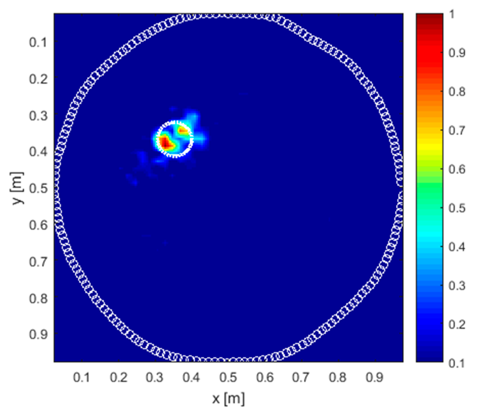
4.1.1. Circular Softwood Tree

The raw data were pre-processed by setting the zero-time of the radar at 1 ns. Time-gating was applied up to 2 ns and was followed by a background removal operation. Figure 6 shows a comparison between raw (Figure 6a) and pre-processed (Figure 6b) data. The presence of the anomaly is identified in the processed data output as a hyperbolic feature located in the right part of the radargram, at a two-way travel time value of about 7 ns.

The microwave tomographic approach was applied on gated data by considering a working frequency band of 800–1800 MHz sampled with 21 frequencies spaced by 50 MHz. The relative dielectric permittivity of the trunk was assumed equal to 17. Note that such a value of permittivity can be regarded as equivalent to the permittivity of a real trunk in a relatively dry environment known to be an inhomogeneous medium consisting of several layers with different electromagnetic properties. The investigation domain was discretised into square pixels with 2.5mm side. The choice of the TSVD is performed by the analysis of the curve of singular values. This was realised by neglecting the singular values below the knee of the curve, where the exponential decay takes place. Therefore, it was decided to truncate the singular values at a threshold of –25 dB with respect to the maximum singular value.

As shown in Figure 7, a number of internal reflections are observed in correspondence of the real target location whereas stronger reflections are present near the surface of the trunk. In order to assess the potentiality of the method in reconstructing the circle-like anomaly only, a more severe time-gating up to 6 ns was applied. The reconstruction results displayed in Figure 8 demonstrate the capability of the tomographic approach for this purpose; in fact, the method is able to locate the defect with good accuracy and in a robust way.

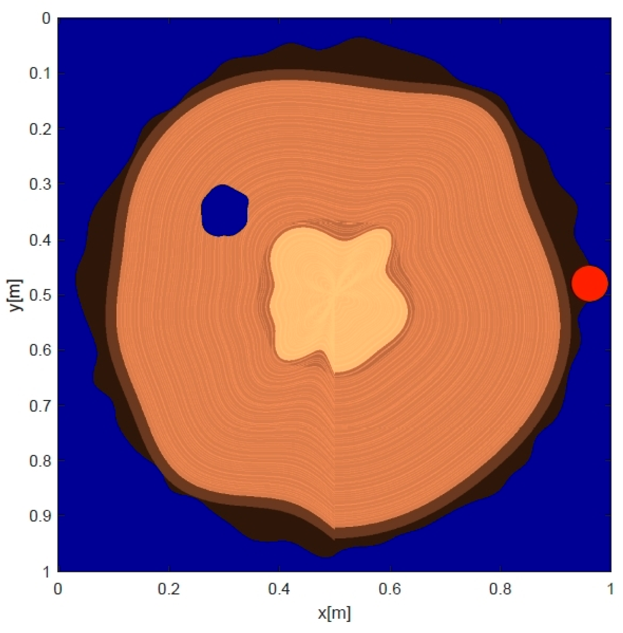
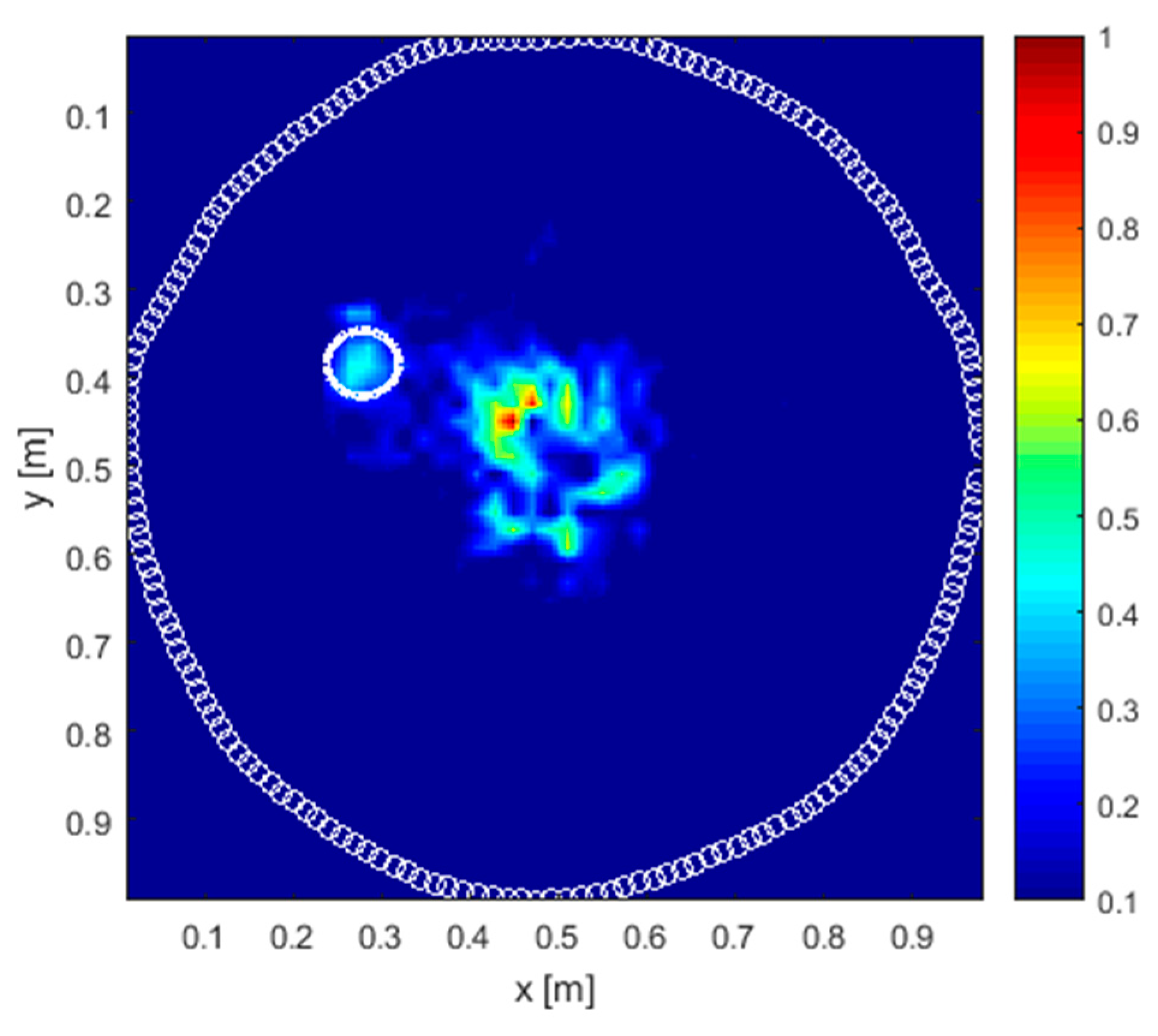
4.1.2. Circular Hardwood Tree

The same pre-processing and reconstruction procedures were applied to the circular hardwood tree scenario shown in Figure 3. In this case, the TSVD threshold was set at −35 dB.

In regard to the pre-processing stage, Figure 9 shows a comparison between raw (Figure 9a) and pre-processed (Figure 9b) data. The use of the proposed preliminary processing stage contributed to clearly identify an hyperbolic feature located at a two-way travel time value of about 5 ns.

As shown in Figure 10, the tomographic reconstruction carried out with a time-gating up to 2 ns proves the potentiality of this method to identify the shape of the hardwood. A weak reflection from the target as well as multiple surface reflections are observed as well. The application of higher time gating (up to 6 ns) in the pre-processing stage allows the identification of the anomaly and the central inner area of the trunk to be improved (see Figure 11).

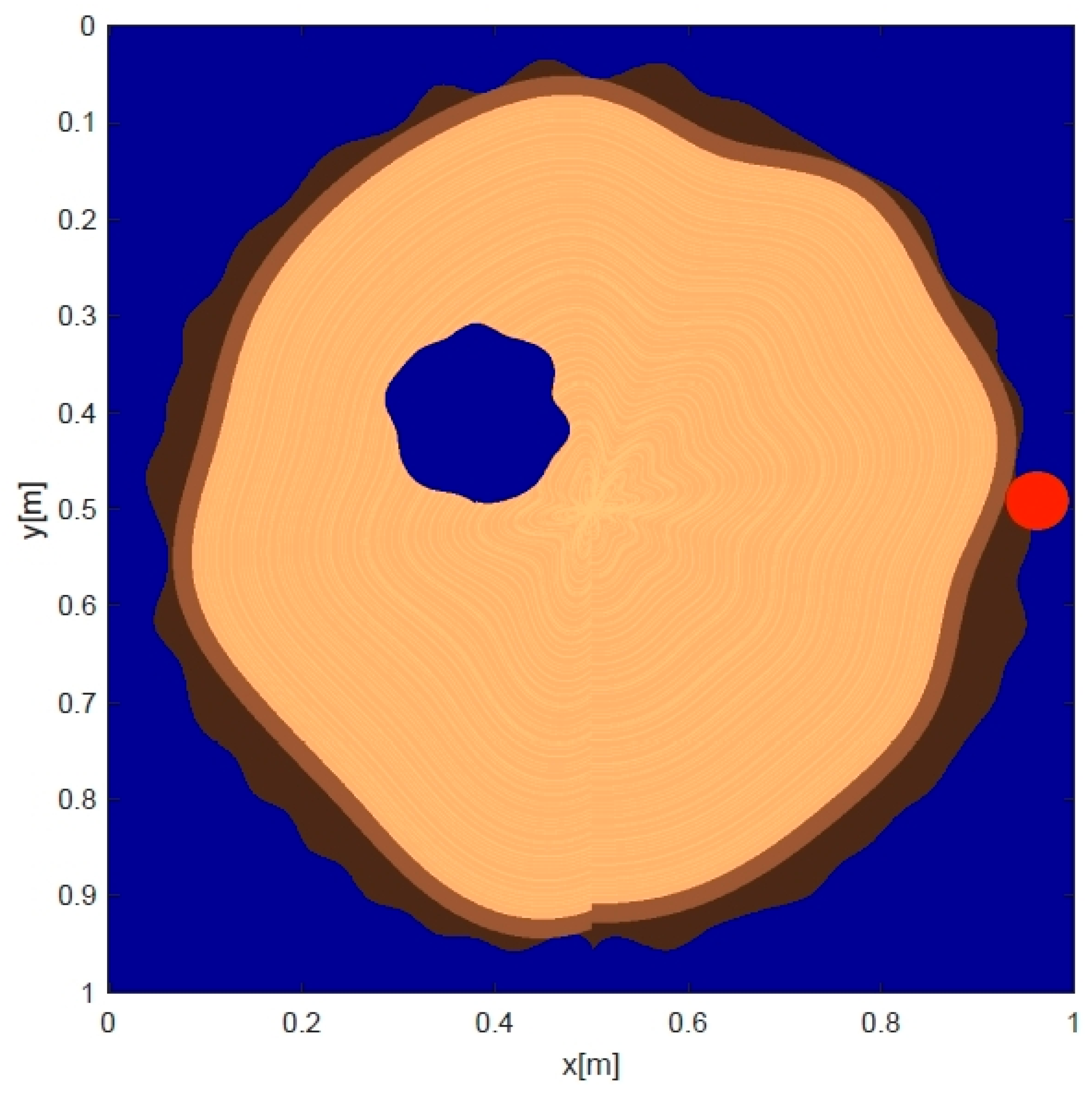
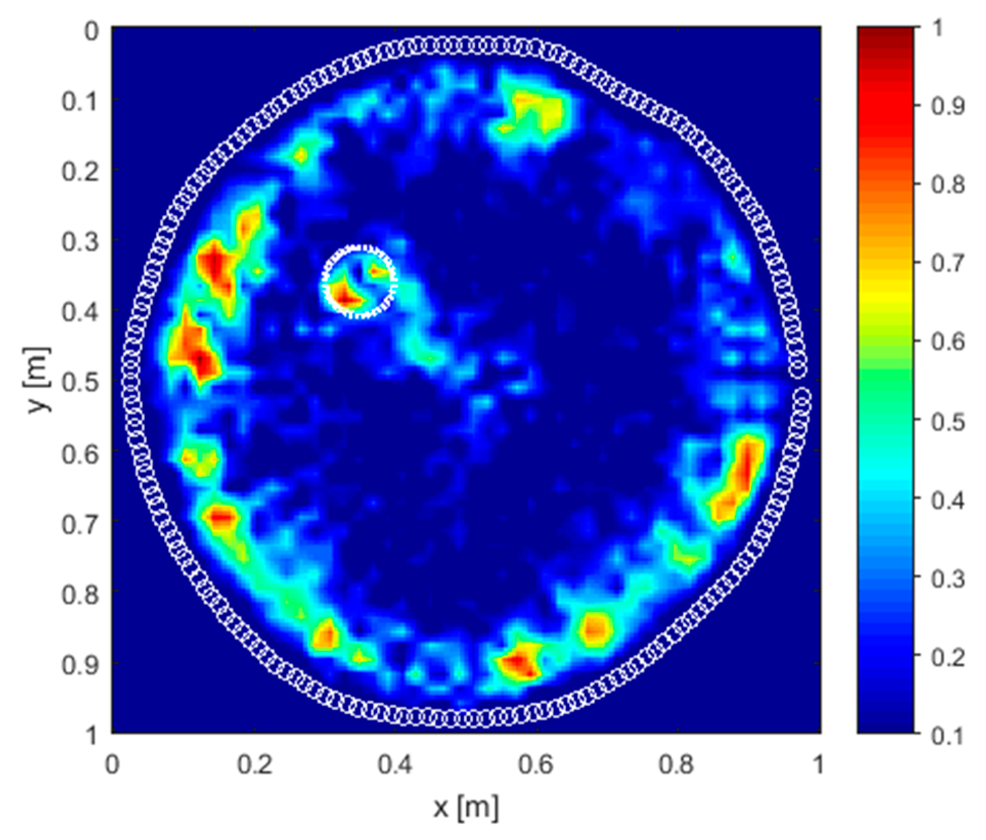
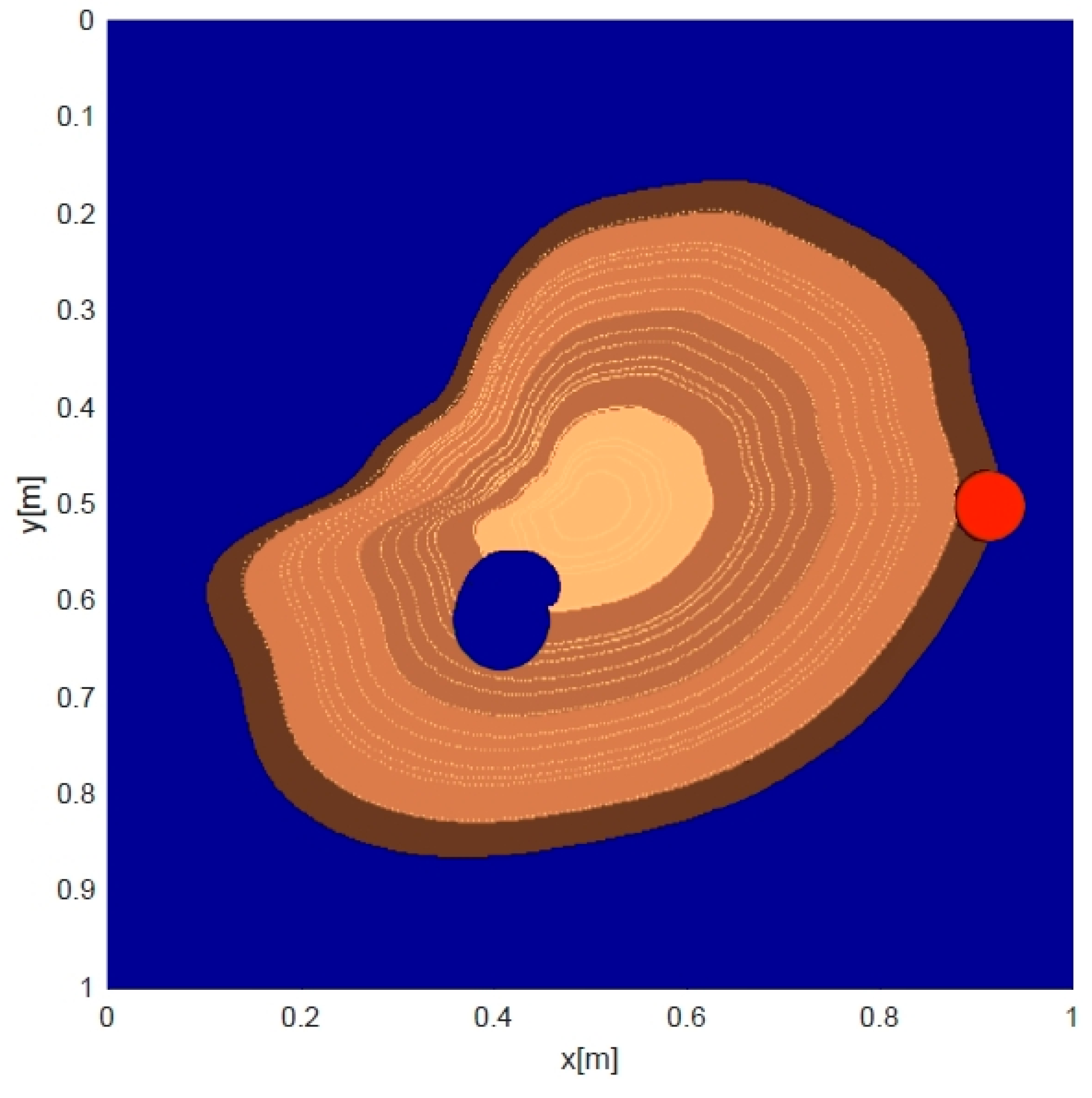
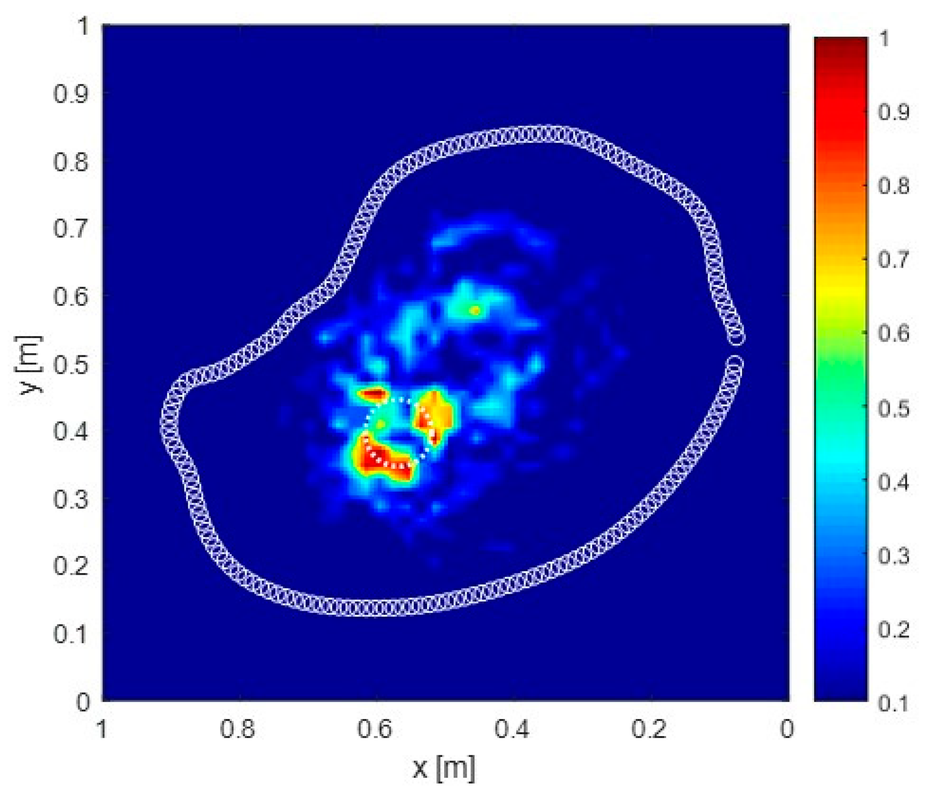
4.1.3. Complex-Shaped Hardwood Tree

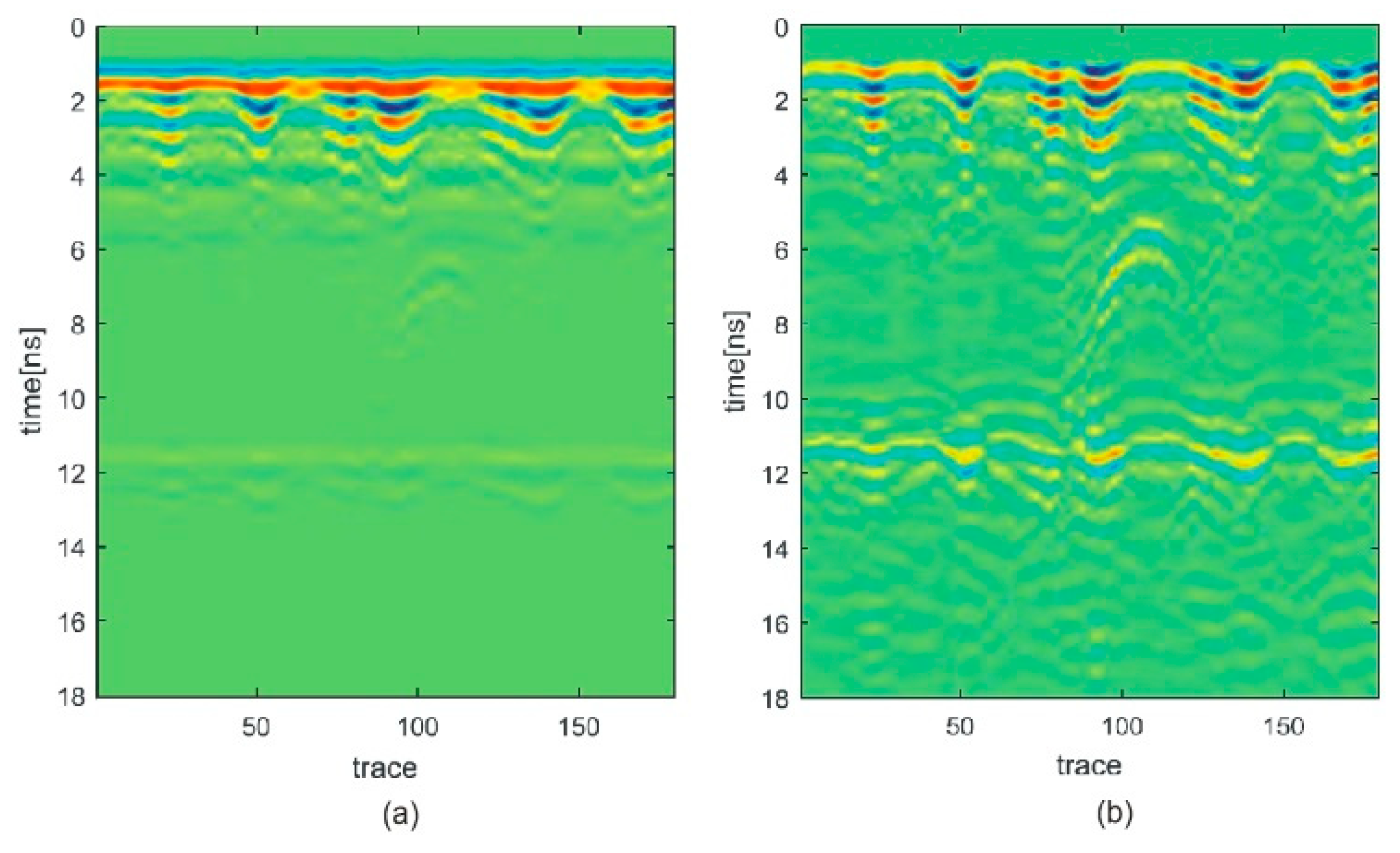
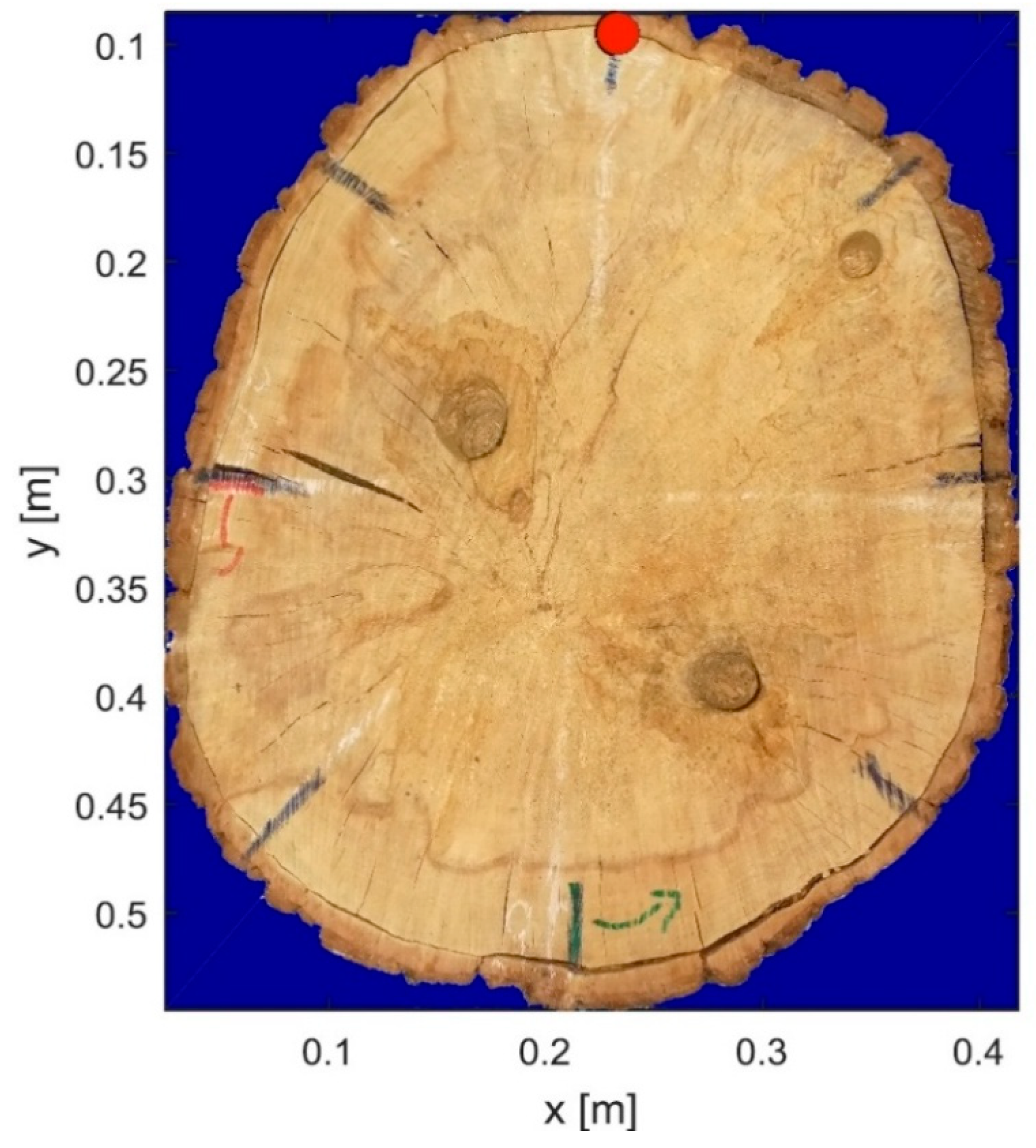
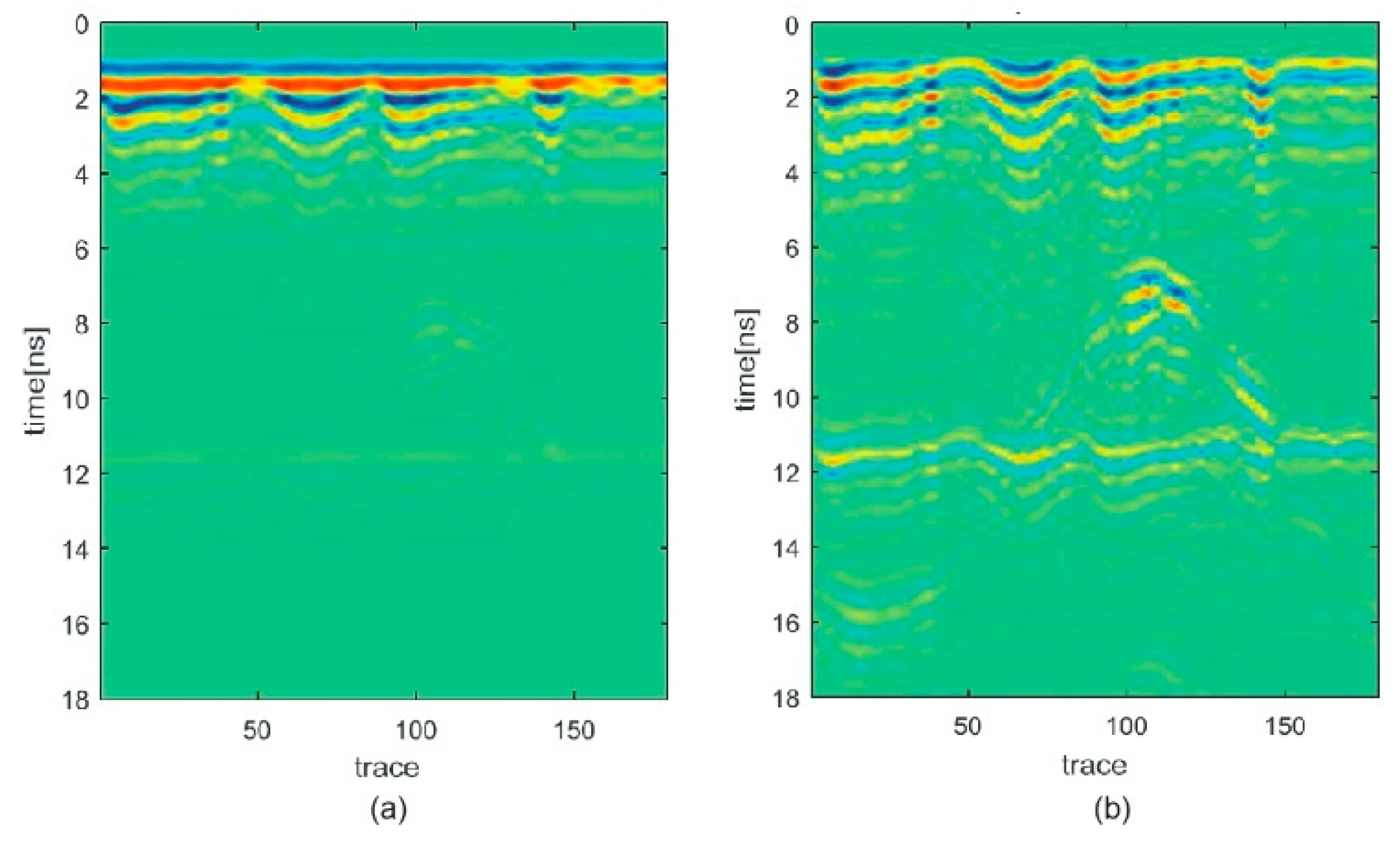
The same pre-processing and tomographic reconstruction schemes used for simulated data were applied to the complex-shaped hardwood tree scenario (Figure 4).

Figure 12 shows a comparison between raw (Figure 12a) and pre-processed (Figure 12b) data. The presence of the anomaly is identified in the processed data output by a hyperbolic feature located in the left-hand side of the radargram, at a two-way travel time value of about 6 ns. However, the presence of several reflections notably complicates the interpretation of the investigated scenario, so motivating the application of the microwave tomographic approach. Such an approach was applied by considering a working frequency band of 800–1800 MHz sampled with 27 frequencies spaced by 38 MHz. The relative dielectric permittivity of the trunk was assumed equal to 17. The TSVD threshold was fixed at −30 dB.

The tomographic reconstruction carried out with a time-gating up to 2 ns is reported in Figure 13, proving the viability in identifying the target, the hardwood and the layer surrounding the hardwood. Most notably, the highest reflection spots are located near the target. A further reconstruction was also performed without time gating, as reported in Figure 14. As a result of this, it is observed that the output is very similar, excluding a new reflection pattern partially visible at the interface between the bark and the first internal layer.

4.2. Real Scenario

The raw data were pre-processed by setting the zero-time at 1.9 ns. Afterwards, time-gating was applied up to 2.7 ns and followed by a background removal operation. Figure 15 shows a comparison between raw (Figure 15a) and pre-processed (Figure 15b) radargrams. The presence of the anomalies is identified in the processed data output by the three hyperbolic features whose apices are located approximately around trace 35, 90, and 120 in the radargram.

The tomographic approach was then applied considering a working frequency band of 1200–2300 MHz sampled with 23 frequencies spaced by 50 MHz. The relative dielectric permittivity of the trunk was estimated equal to 5 by measuring the two-way travel time associated to the reflection from the opposite side of the trunk. The TSVD threshold was fixed at −30 dB.

The tomographic reconstruction reported in Figure 16 turns out to be effective in identifying the three targets. It is worthy of note that the highest reflections are observed towards the bark, whereas the most internal reflection is more attenuated.

5. Conclusion and Future Research

This paper reports a demonstration of the potential of ground penetrating radar (GPR) and the use of a tomographic inversion approach in detecting decay and cavities in tree trunks. To this effect, a set of Finite-Difference Time-Domain (FDTD) simulations of different complexity was used and after the method was validated on a real trunk with several decay.

The radar signals demonstrate that the method is capable of identifying signs of inner reflections at the location point of the anomaly in a tree. Concerning the outputs of the numerical simulations, detection becomes more accurate in round-shaped trunks if more severe time-gating is applied to the signal in the time domain. This is particularly relevant for identifying cavities and decay located towards the inner section of a trunk. In the case of more complex-shaped trunks, the results of the simulations show that an effective detection of the target can be achieved as well.

The application of the tomographic inversion approach to a real trunk with several areas of decay was proven effective in identifying all the targets. It was observed that the reflections from targets closer to the bark are stronger than the reflections from targets located more internally in the cross-section.

Future research could task itself with the application of the tomographic inversion approach to further complex numerical scenarios, and living tree trunks of different dimensions and species under varying health conditions. A further factor that could be considered in this study is the optimal choice of the operating frequency of the GPR system in the case of living trees, which in turn is crucial in view of the large variability of both the dielectric permittivity and the electrical conductivity of the probed medium.

References

1. Pan, Y.; Birdsey, A.B.; Fang, J.; Houghton, R.; Kauppi, P.E.; Kurz, A.K.; Phillips, O.L.; Shvidenko, A.; Lewis, S.L.; Canadell, J.G.; et al. A Large and Persistent Carbon Sink in the World’s Forests. Science 2011, 333, 988–993. [Google Scholar] [CrossRef] [PubMed]
2. Hansen, E.M.; Goheen, E.M. Phellinus weirii and other native root pathogens as determinants of forest structure and process in western North America. Ann. Rev. Phytopathol. 2000, 38, 515–539. [Google Scholar] [CrossRef] [PubMed]
3. Richardson, D.M.; Pyšek, P.; Rejmánek, M.; Barbour, M.G.; Panetta, F.D.; West, C.J. Naturalization and invasion of alien plants: Concepts and definitions. In Diversity and Distributions; Wiley Online Library: Berlin, Germany, 2001; pp. 93–107. [Google Scholar]
4. Santini, A.; Ghelardini, L.; De Pace, C.; Desprez-Loustau, M.L.; Capretti, P.; Chandelier, A.; Cech, T.; Chira, D.; Diamandis, S.; Gaitniekis, T.; et al. Biogeographical patterns and determinants of invasion by forest pathogens in Europe. New Phytol. 2012, 197, 238–250. [Google Scholar] [CrossRef] [PubMed] [Green Version]
5. Guo, Q.; Rejmanek, M.; Wen, J. Geographical, socioeconomic, and ecological determinants of exotic plant naturalization in the United States: Insights and updates from improved data. NeoBiota 2012, 12, 41–55. [Google Scholar] [CrossRef]
6. Liebhold, A.M.; Brockerhoff, E.G.; Garrett, L.J.; Parke, J.L.; Britton, K.O. Live plant imports: The major pathway for forest insect and pathogen invasions of the US. Front. Ecol. Env. 2012, 10, 135–143. [Google Scholar] [CrossRef]
7. Broome, A.; Ray, D.; Mitchell, R.; Harmer, R. Responding to ash dieback (Hymenoscyphus fraxineus) in the UK: Woodland composition and replacement tree species. Forestry 2019, 92, 108–119. [Google Scholar] [CrossRef]
8. Jung, T. Beech decline in Central Europe driven by the interaction between Phytophthora infections and climatic extremes. In Forest Pathology; Wiley Online Library: Berlin, Germany, 2009; pp. 73–94. [Google Scholar]
9. Anderson, P.K.; Cunningham, A.A.; Patel, N.G.; Morales, F.J.; Epstein, P.R.; Daszak, P. Emerging infectious diseases of plants: Pathogen pollution, climate change and agrotechnology drivers. Trends Ecol. Evol. 2004, 19, 535–544. [Google Scholar] [CrossRef]
10. Daszak, P. Emerging Infectious Diseases of Wildlife—Threats to Biodiversity and Human Health. Science 2000, 287, 443–449. [Google Scholar] [CrossRef]
11. Fisher, M.C.; Henk, D.A.; Briggs, C.J.; Brownstein, J.S.; Madoff, L.C.; McCraw, S.L.; Gurr, S.J. Emerging fungal threats to animal, plant and ecosystem health. Nature 2012, 484, 186–194. [Google Scholar] [CrossRef] [PubMed]
12. Potter, C.; Harwood, T.; Knight, J.; Tomlinson, I. Learning from history, predicting the future: The UK Dutch elm disease outbreak in relation to contemporary tree disease threats. Philos. Trans. R. Soc. B Boil. Sci. 2011, 366, 1966–1974. [Google Scholar] [CrossRef]
13. McMullan, M.; Rafiqi, M.; Kaithakottil, G.; Clavijo, B.J.; Bilham, L.; Orton, E.; Percival-Alwyn, L.; Ward, B.J.; Edwards, A.; Saunders, D.G.O.; et al. The ash dieback invasion of Europe was founded by two genetically divergent individuals. Nat. Ecol. Evol. 2018, 2, 1000–1008. [Google Scholar] [CrossRef] [PubMed] [Green Version]
14. Brown, N.; Inward, D.J.G.; Jeger, M.; Denman, S. A review of Agrilus biguttatus in UK forests and its relationship with acute oak decline. For. Int. J. For. Res. 2015, 88, 53–63. [Google Scholar] [CrossRef]
15. Gibbs, J.N. Intercontinental Epidemiology of Dutch Elm Disease. Ann. Rev. Phytopathol. 1978, 16, 287–307. [Google Scholar] [CrossRef]
16. Papic, S.; Longauer, R.; Milenković, I.; Rozsypálek, J. Genetic predispositions of common ash to the ash dieback caused by ash dieback fungus. Genetika 2018, 50, 221–229. [Google Scholar] [CrossRef] [Green Version]
17. Worrell, R. An Assessment of the Potential Impacts of Ash Dieback in Scotland. Available online: https://bit.ly/2ZkYhNc (accessed on 30 August 2019).
18. Brown, N. Epidemiology of Acute Oak Decline in Great Britain. Available online: https://spiral.imperial.ac.uk/handle/10044/1/30827 (accessed on 30 August 2019).
19. Brasier, C.M. Dual origin of recent Dutch elm disease outbreaks in Europe. Nature 1979, 281, 78–80. [Google Scholar] [CrossRef]
20. Brasier, C.M.; Gibbs, J.N. Origin of the Dutch Elm Disease Epidemic in Britain. Nature 1973, 242, 607–609. [Google Scholar] [CrossRef]
21. Denman, S.; Brown, N.; Kirk, S.; Jeger, M.; Webber, J. A description of the symptoms of Acute Oak Decline in Britain and a comparative review on causes of similar disorders on oak in Europe. Forestry 2014, 87, 535–551. [Google Scholar] [CrossRef] [Green Version]
22. Ouis, D. Non destructive techniques for detecting decay in standing trees. Arboric. J. 2003, 27, 159–177. [Google Scholar] [CrossRef]
23. Winistorfer, P.M.; Xu, W.; Wimmer, R. Application of A Drill Resistance Technique for Density Profile Measurement in Wood Composite Panels. Available online: https://bit.ly/2zymrVm (accessed on 30 August 2019).
24. Schwarze, F.W.M.R.; Ferner, D. Ganoderma on trees—Differentiation of species and studies of invasiveness. Arboric. J. 2003, 27, 59–77. [Google Scholar] [CrossRef]
25. Shortle, W.C.; Dudzik, K.R. Wood Decay in Living and Dead Trees: A Pictorial Overview. Available online: https://www.fs.usda.gov/treesearch/pubs/40899 (accessed on 30 August 2019).
26. Costello, L.; Quarles, S. Detection of wood decay in blue gum and elm: An evaluation of the Resistograph and the portable drill. J. Arboric. 1999, 25, 311–317. [Google Scholar]
27. Al Hagrey, S.A. Electrical resistivity imaging of tree trunks. Near Surf. Geophys. 2006, 4, 179–187. [Google Scholar] [CrossRef]
28. Deflorio, G.; Fink, S.; Schwarze, F.W. Detection of incipient decay in tree stems with sonic tomography after wounding and fungal inoculation. Wood Sci. Technol. 2008, 42, 117–132. [Google Scholar] [CrossRef]
29. Catena, A. Thermography shows damaged tissue and cavities present in trees. Nondestruct. Charact. Mater. 2003, 11, 515–522. [Google Scholar]
30. Wei, Q.; Leblon, B.; Rocque, L.A. On the use of X-ray computed tomography for determining wood properties: A review. Can. J. Forest Res. 2011, 41, 2120–2140. [Google Scholar] [CrossRef]
31. Boero, F.; Fedeli, A.; Lanini, M.; Maffongelli, M.; Monleone, R.; Pastorino, M.; Randazzo, A.; Salvadè, A.; Sansalone, A. Microwave Tomography for the Inspection of Wood Materials: Imaging System and Experimental Results. IEEE Trans. Microw. Theory Tech. 2018, 66, 3497–3510. [Google Scholar] [CrossRef]
32. Goodman, D. Ground-penetrating radar simulation in engineering and archaeology. Geophysics 1994, 59, 224–232. [Google Scholar] [CrossRef]
33. Catapano, I.; Gennarelli, G.; Ludeno, G.; Soldovieri, F. Applying Ground-Penetrating Radar and Microwave Tomography Data Processing in Cultural Heritage: State of the art and future trends. IEEE Signal. Process. Mag. 2019, 36, 53–61. [Google Scholar] [CrossRef]
34. Giannakis, I.; Giannopoulos, A.; Yarovoy, A. Model-Based Evaluation of Signal-to-Clutter Ratio for Landmine Detection Using Ground-Penetrating Radar. IEEE Trans. Geosci. Remote. Sens. 2016, 54, 1–10. [Google Scholar] [CrossRef]
35. González-Huici, M.A.; Catapano, I.; Soldovieri, F. A Comparative Study of GPR Reconstruction Approaches for Landmine Dete. IEEE J. Sel. Top. Appl. Earth Obs. Remote Sens. 2014, 7, 4869–4878. [Google Scholar] [CrossRef]
36. Alani, A.M.; Tosti, F. GPR applications in structural detailing of a major tunnel using different frequency antenna systems. Constr. Build. Mater. 2018, 158, 1111–1122. [Google Scholar] [CrossRef]
37. Lo Monte, L.; Erricolo, D.; Soldovieri, F.; Wicks, M.C. Radio frequency tomography for tunnel detection. IEEE Trans. Geosci. Remote Sens. 2009, 48, 1128–1137. [Google Scholar] [CrossRef]
38. Alani, A.M.; Aboutalebi, M.; Kilic, G. Applications of ground penetrating radar (GPR) in bridge deck monitoring and assessment. J. Appl. Geophys. 2013, 97, 45–54. [Google Scholar] [CrossRef]
39. Benedetto, A.; Pajewski, L. Civil Engineering Applications of Ground Penetrating Radar. Available online: https://bit.ly/2Zn6lwZ (accessed on 30 August 2019).
40. Tosti, F.; Ciampoli, L.B.; D’Amico, F.; Alani, A.M.; Benedetto, A. An experimental-based model for the assessment of the mechanical properties of road pavements using ground-penetrating radar. Constr. Build. Mater. 2018, 165, 966–974. [Google Scholar] [CrossRef]
41. Catapano, I.; Ludeno, G.; Soldovieri, F.; Tosti, F.; Padeletti, G. Structural Assessment via Ground Penetrating Radar at the Consoli Palace of Gubbio (Italy). Remote Sens. 2018, 10, 45. [Google Scholar] [CrossRef]
42. Tosti, F.; Pajewski, L. Applications of Radar Systems in Planetary Sciences: An Overview; Benedetto, A., Pajewski, L., Eds.; Civil Engineering Applications of Ground Penetrating Radar; Springer Transactions in Civil and Environmental Engineering; Springer: Cham, Switzerland, 2015; pp. 361–371. [Google Scholar]
43. Orosei, R.; Lauro, S.E.; Pettinelli, E.; Cicchetti, A.; Coradini, M.; Cosciotti, B.; Di Paolo, F.; Flamini, E.; Mattei, E.; Pajola, M.; et al. Radar evidence of subglacial liquid water on Mars. Science 2018, 361, 490–493. [Google Scholar] [CrossRef] [PubMed] [Green Version]
44. Carrer, L.; Bruzzone, L. Solving for ambiguities in radar geophysical exploration of planetary bodies by mimicking bats echolocation. Nat. Commun. 2017, 8, 2248. [Google Scholar] [CrossRef] [PubMed]
45. Davis, J.L.; Annan, A.P. Ground-penetrating radar for high-resolution mapping of soil and rock stratigraphy. Geophys. Prospect. 1989, 37, 531–551. [Google Scholar] [CrossRef]
46. Tosti, F.; Slob, E. Determination, by Using GPR, of the Volumetric Water Content in Structures, Substructures, Foundations and Soil. In Civil Engineering Applications of Ground Penetrating Radar. Springer Transactions in Civil and Environmental Engineering; Benedetto, A., Pajewski, L., Eds.; Springer: Cham, Switzerland, 2015; pp. 163–194. [Google Scholar]
47. Brunzell, H. Detection of shallowly buried objects using impulse radar. IEEE Trans. Geosci. Remote. Sens. 1999, 37, 875–886. [Google Scholar] [CrossRef] [Green Version]
48. Ambrosanio, M.; Bevacqua, M.T.; Isernia, T.; Pascazio, V. The Tomographic Approach to Ground-Penetrating Radar for Underground Exploration and Monitoring: A more user-friendly and unconventional method for subsurface investigation. IEEE Signal. Process. Mag. 2019, 36, 62–73. [Google Scholar] [CrossRef]
49. Fedeli, A.; Jezova, J.; Lambot, S.; Pastorino, M.; Randazzo, A. Nonlinear Inversion of Multifrequency GPR Data in Tomographic Configurations. In Geophysical Research Abstracts. Available online: https://bit.ly/2zwN1hx (accessed on 30 August 2019).
50. Nicolotti, G.; Socco, L.V.; Martinis, R.; Godio, A.; Sambuelli, L. Application and comparison of three tomographic techniques for detection of decay in trees. J. Arboric. 2003, 29, 66–78. [Google Scholar]
51. Lorenzo, H.; Perez-Gracia, V.; Novo, A.; Armesto, J. Forestry applications of ground-penetrating radar. For. Syst. 2010, 19, 5–17. [Google Scholar] [CrossRef]
52. Ježová, J.; Mertens, L.; Lambot, S. Ground-penetrating radar for observing tree trunks and other cylindrical objects. Constr. Build. Mater. 2016, 123, 214–225. [Google Scholar] [CrossRef]
53. Jezova, J.; Harou, J.; Lambot, S. Reflection waveforms occurring in bistatic radar testing of columns and tree trunks. Constr. Build. Mater. 2018, 174, 388–400. [Google Scholar] [CrossRef]
54. Al Hagrey, S.A. Geophysical imaging of root-zone, trunk, and moisture heterogeneity. J. Exp. Bot. 2007, 58, 839–854. [Google Scholar] [CrossRef] [Green Version]
55. Alani, A.; Ciampoli, L.B.; Lantini, L.; Tosti, F.; Benedetto, A. Mapping the Root System Of Matured Trees Using Ground Penetrating Radar. Available online: https://bit.ly/2lB3cXa (accessed on 3 September 2019).
56. Tosti, F.; Bianchini Ciampoli, L.; Brancadoro, M.G.; Alani, A.M. GPR applications in mapping the subsurface root system of street trees with road safety-critical implications. Adv. Transp. Stud. 2018, 44, 107–118. [Google Scholar]
57. Lantini, L.; Holleworth, R.; Egyir, D.; Giannakis, I.; Tosti, F.; Alani, A. Use of Ground Penetrating Radar for Assessing Interconnections between Root Systems of Different Matured Tree Species. Available online: https://repository.uwl.ac.uk/id/eprint/5491/ (accessed on 30 August 2019).
58. Giannakis, I.; Tosti, F.; Lantini, L.; Alani, A.M. Health Monitoring of Tree Trunks Using Ground Penetrating Radar. IEEE Trans. Geosci. Remote. Sens. 2019, 1–10. [Google Scholar] [CrossRef]
59. Alani, A.; Bianchini Ciampoli, L.; Tosti, F.; Brancadoro, M.G.; Pirrone, D.; Benedetto, A. Health Monitoring of a Matured Tree Using Ground Penetrating Radar–Investigation of the Tree Root System and Soil Interaction. Available online: https://repository.uwl.ac.uk/id/eprint/3913/ (accessed on 30 August 2019).
60. Pastorino, M. Microwave Imaging; John Wiley & Sons, Inc.: Hoboken, NJ, USA, 2010. [Google Scholar]
61. Miao, Z.; Kosmas, P. Multiple-frequency DBIM-TwIST algorithm for microwave breast imaging. IEEE Trans. Antennas Propag. 2017, 65, 1. [Google Scholar] [CrossRef]
62. Gilmore, C.; Abubakar, A.; Hu, W.; Habashy, T.M.; Berg, P.M.V.D. Microwave Biomedical Data Inversion Using the Finite-Difference Contrast Source Inversion Method. IEEE Trans. Antennas Propag. 2009, 57, 1528–1538. [Google Scholar] [CrossRef]
63. Leucci, G.; Masini, N.; Persico, R.; Soldovieri, F. GPR and sonic tomography for structural restoration: The case of the cathedral of Tricarico. J. Geophys. Eng. 2011, 8, S76–S92. [Google Scholar] [CrossRef]
64. Daniels, D.J. Ground Penetrating Radar. Available online: https://bit.ly/2LfZr2F (accessed on 30 August 2019).
65. Catapano, I.; Gennarelli, G.; Ludeno, G.; Soldovieri, F.; Persico, R. Ground-Penetrating Radar: Operation Principle and Data Processing. Available online: https://bit.ly/2lVMmmi (accessed on 3 September 2019).
66. Benedetto, A.; Tosti, F.; Ciampoli, L.B.; D’Amico, F. An overview of ground-penetrating radar signal processing techniques for road inspections. Signal. Process. 2017, 132, 201–209. [Google Scholar] [CrossRef]
67. Soldovieri, F.; Solimene, R. Ground Penetrating Radar Subsurface Imaging of Buried. Available online: Objectshttps://bit.ly/2lvPNA0 (accessed on 30 August 2019).
68. Persico, R. Introduction to Ground Penetrating Radar: Inverse Scattering and Data Processing. Available online: https://bit.ly/2UlBjQy (accessed on 30 August 2019).
69. Solimene, R.; Catapano, I.; Gennarelli, G.; Cuccaro, A.; Dell’Aversano, A.; Soldovieri, F. SAR Imaging Algorithms and Some Unconventional Applications: A unified mathematical overview. IEEE Signal. Process. Mag. 2014, 31, 90–98. [Google Scholar] [CrossRef]
70. Bertero, M.; Boccacci, P. Introduction to Inverse Problems in Imaging. Available online: https://bit.ly/2lTr2Og (accessed on 30 August 2019).
71. Persico, R.; Bernini, R.; Soldovieri, F. The role of the measurement configuration in inverse scattering from buried objects under the Born approximation. IEEE Trans. Antennas Propag. 2005, 53, 1875–1887. [Google Scholar] [CrossRef]
72. Warren, C.; Giannopoulos, A.; Giannakis, I. gprMax: Open source software to simulate electromagnetic wave propagation for Ground Penetrating Radar. Comput. Phys. Commun. 2016, 209, 163–170. [Google Scholar] [CrossRef] [Green Version]
73. Giannakis, I.; Giannopoulos, A.; Warren, C.; Warren, C. Realistic FDTD GPR antenna models optimized using a novel linear/nonlinear Full-Waveform Inversion. IEEE Trans. Geosci. Remote. Sens. 2018, 57, 1768–1778. [Google Scholar] [CrossRef]
Figure 1. Geometry of a tree cross-section with an arbitrary shape. The red circles represent the Ground Penetrating Radar (GPR) measurement points along the outer surface of the bark; the white object is a randomly-positioned target within the cross-section.
Remotesensing 11 02073 g001
Figure 2. The circular softwood trunk scenario investigated using Finite-Difference Time-Domain (FDTD) numerical modelling. The starting point of the measurements, taken clockwise, is represented by the red circle.
Remotesensing 11 02073 g002
Figure 3. The circular hardwood trunk scenario investigated using FDTD numerical modelling. The starting point of the measurements, taken clockwise, is represented by the red circle.
Remotesensing 11 02073 g003
Figure 4. The complex-shaped hardwood trunk scenario investigated using FDTD numerical modelling. The starting point of the measurements, taken clockwise, is represented by the red circle.
Remotesensing 11 02073 g004
Figure 5. The oak tree trunk investigated at The Faringdon Centre-Non-Destructive Testing Centre, University of West London (UWL), UK. Measurements were taken counter-clockwise and the red circle denotes the starting point.
Remotesensing 11 02073 g005
Figure 6. Radargrams of the simulations for the softwood tree scenario. (a) Raw radargam; (b) processed radargram after the application of the pre-processing stage.
Remotesensing 11 02073 g006
Figure 7. Tomographic reconstruction of the softwood scenario with time-gating up to 2 ns. The dashed white circle indicates the actual position of the anomaly. The circles in white solid line along the trunk perimeter represent the positions of the measurement points.
Remotesensing 11 02073 g007
Figure 8. Tomographic reconstruction of the softwood scenario with time-gating up to 6 ns. The dashed white circle indicates the actual position of the anomaly. The circles in white solid line along the trunk perimeter represent the positions of the measurement points.
Remotesensing 11 02073 g008
Figure 9. Radargrams of the simulations for the circular hardwood tree scenario. (a) Raw radargam; (b) processed radargram after the application of the pre-processing stage.
Remotesensing 11 02073 g009
Figure 10. Tomographic reconstruction of the circular hardwood tree scenario with time-gating up to 2 ns. The circles in white solid line along the trunk perimeter represent the positions of the measurement points.
Remotesensing 11 02073 g010
Figure 11. Tomographic reconstruction of the circular hardwood tree scenario with time-gating up to 6 ns. The dashed white circle indicates the actual position of the anomaly. The circles in white solid line along the trunk perimeter represent the positions of the measurement points.
Remotesensing 11 02073 g011
Figure 12. Radargrams of the simulations for the complex-shaped hardwood tree scenario. (a) Raw radargam; (b) processed radargram after the application of the pre-processing stage.
Remotesensing 11 02073 g012
Figure 13. Tomographic reconstruction of the complex-shaped hardwood tree scenario with time-gating up to 2 ns. The dashed white circle indicates the actual position of the anomaly. The circles in white solid line along the trunk perimeter represent the positions of the measurement points.
Remotesensing 11 02073 g013
Figure 14. Tomographic reconstruction of the complex-shaped hardwood tree scenario without the application of time-gating. The dashed white circle indicates the actual position of the anomaly. The circles in white solid line along the trunk perimeter represent the positions of the measurement points.
Remotesensing 11 02073 g014
Figure 15. Radargrams of the real tree scenario. (a) Raw radargam; (b) processed radargram after the application of the pre-processing stage.
Remotesensing 11 02073 g015
Figure 16. Tomographic reconstruction of the real tree scenario. The dashed white circles indicate the actual position of the anomalies. The circles in white solid line along the trunk perimeter represent the positions of the measurement points.
Remotesensing 11 02073 g016