Spectral and Radiometric Calibration of the Next Generation Airborne Visible Infrared Spectrometer (AVIRIS-NG)

Abstract

We describe advanced spectral and radiometric calibration techniques developed for NASA’s Next Generation Airborne Visible Infrared Imaging Spectrometer (AVIRIS-NG). By employing both statistically rigorous analysis and utilizing in situ data to inform calibration procedures and parameter estimation, we can dramatically reduce undesirable artifacts and minimize uncertainties of calibration parameters notoriously difficult to characterize in the laboratory. We describe a novel approach for destriping imaging spectrometer data through minimizing a Markov Random Field model. We then detail statistical methodology for bad pixel correction of the instrument, followed by the laboratory and field protocols involved in the corrections and evaluate their effectiveness on historical data. Finally, we review the geometric processing procedure used in production of the radiometrically calibrated image data.

1. Introduction

Remote imaging spectroscopy, also known as hyperspectral imaging, leverages the unique interactions between matter and electromagnetic radiation to analyze Earth’s environment through the physical, biological, and chemical information present in spectral reflectance and absorptions. In particular, imaging spectrometers covering the Visible/ShortWave InfraRed (VSWIR) portion of the spectrum capture a majority of the solar reflectance and enable Earth science investigations across a wide range of fields [1].

Typical spectral calibration procedures begin by the translating raw digital numbers (DNs) to units of radiant intensity measured at the sensor. This requires understanding both the instrument radiometric response and the spectral response of each instrument channel. The accuracy of these initial calibration steps is critical since any uncertainties present at this stage propagate to all subsequent products. While laboratory calibration procedures have been refined for decades, campaigns often incorporate in-flight data to estimate instrument parameters that are difficult to characterize in the lab, such as atmospheric effects [2].

In the study that follows, we detail the motivation and operation of advanced calibration procedures developed for the National Aeronautics and Space Administration (NASA)’s Next Generation Airborne Visible Infrared Imaging Spectrometer (AVIRIS-NG) instrument. We then describe the laboratory and vicarious calibration/validation procedures used during the analysis. Finally we validate the improved calibration procedures through historical data and describe the geometric processing procedure.

Instrument

NASA’s AVIRIS-NG is a pushbroom spectral mapping system with high signal-to-noise ratio (SNR), designed and toleranced for high performance spectroscopy. AVIRIS-NG was developed as a successor to the Classic Airborne Visible Infrared Imaging Spectrometer (AVIRIS-C) [3]. The instrument covers the entire solar reflected spectrum, 380–2510 nm range with a single Focal Plane Array (FPA), at a spectral sampling of approximately 5 nm. The AVIRIS-NG sensor has a 1 milliradian instantaneous field of view, providing altitude-dependent ground sampling distances from 20 m to the sub-meter range. To date, it has flown on diverse aircraft platforms including the Twin Otter, the King Air B-200, and NASA’s high altitude ER-2. Its detector has a 640 × 480 pixel array, from which standard products are generated using the sensor’s 600 cross-track spatial samples and 425 spectral samples.

AVIRIS-NG data uncertainties come from natural and irreducible measurement noise, but others are calibration uncertainties that arise from systematic optical and electronic imperfections in the instrument. These systematic imperfections are amenable to characterization and correction, and any final data product analytic impact they may have is relatively small due to careful optical design that promotes uniformity and alignment. For AVIRIS-NG, optical errors can be further categorized into radiometric and spectral measurement errors. Of those, community experience has shown that instrument spectral accuracy has the greatest likelihood of impacting surface chemistry data products. Overall scene radiometry is facet and sun-angle dependent, but since spectroscopic analyses typically rely on relative shapes of spectra, their accuracy can often tolerate a degree of gray instrumental offset, i.e., absolute radiometric error with no spectral component.

The nature of electronically induced errors are unique to the detection system of AVIRIS-NG. The photon-to-DN electronic chain of AVIRIS-NG consists of a Focal Plane Array, Teledyne imaging sensor comprised of a homogeneous HgCdTe photodetector wafer connected to its Read Out Integrated Circuit (ROIC) via a 640 × 480 array of conductive “bump” bonds, shielded ribbon cables routing FPA serial analog voltage and timing signals to the outside of the instrument vacuum can, and external A/D conversion by a custom Focal Plane Integration Electronics module. This electronic chain has a degree of inherent noise as well as systematic artifacts. These artifacts are both environmentally dependent and scene dependent, but are generally stable enough in their overall behavior to be characterized and corrected.

2. Materials and Methods

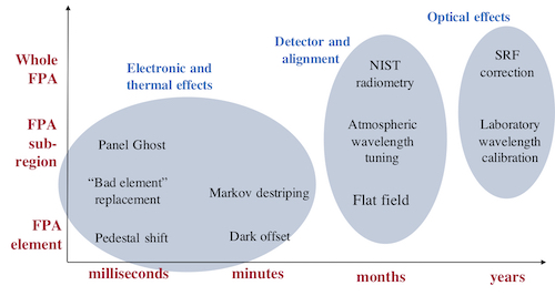
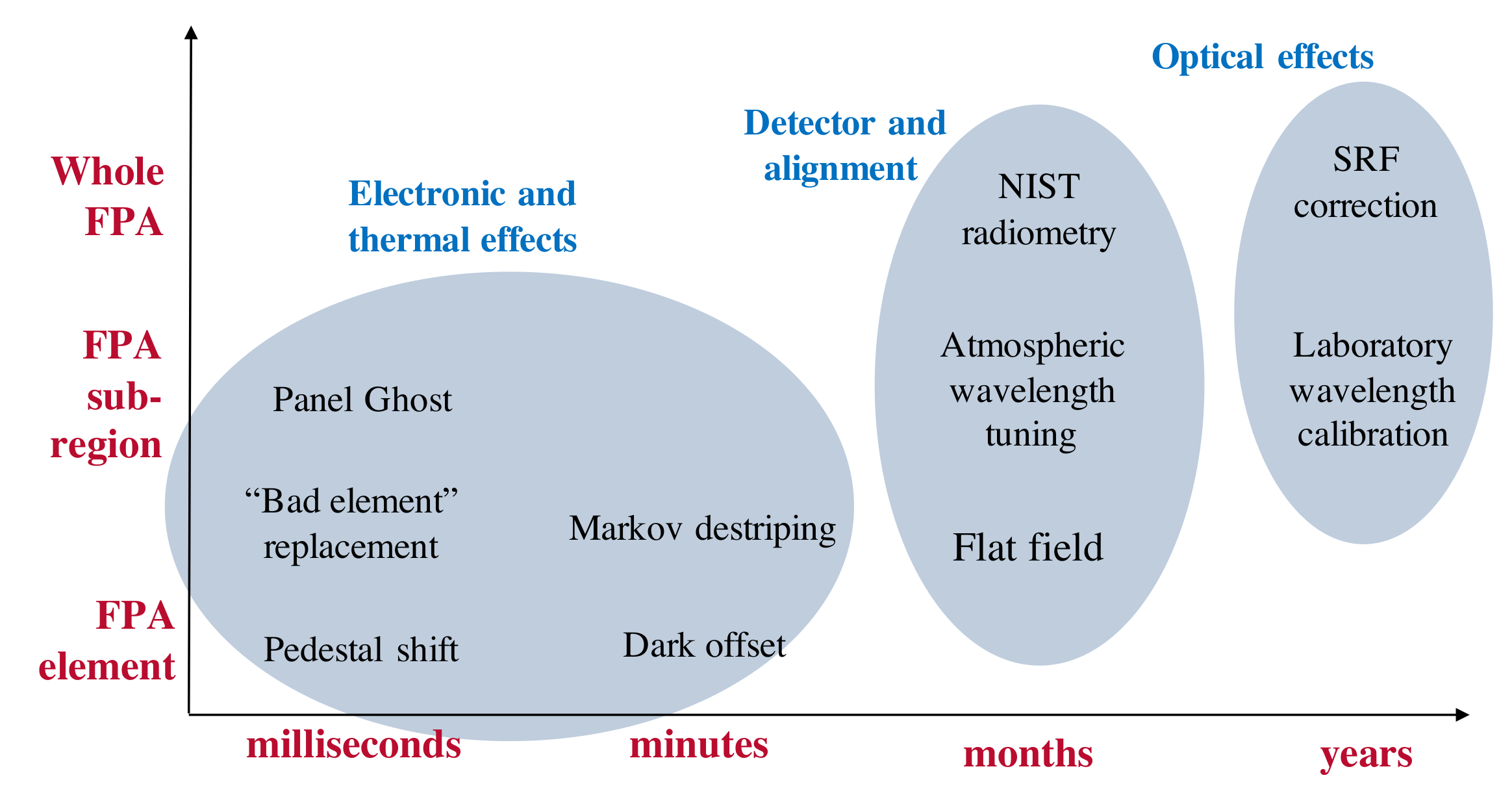
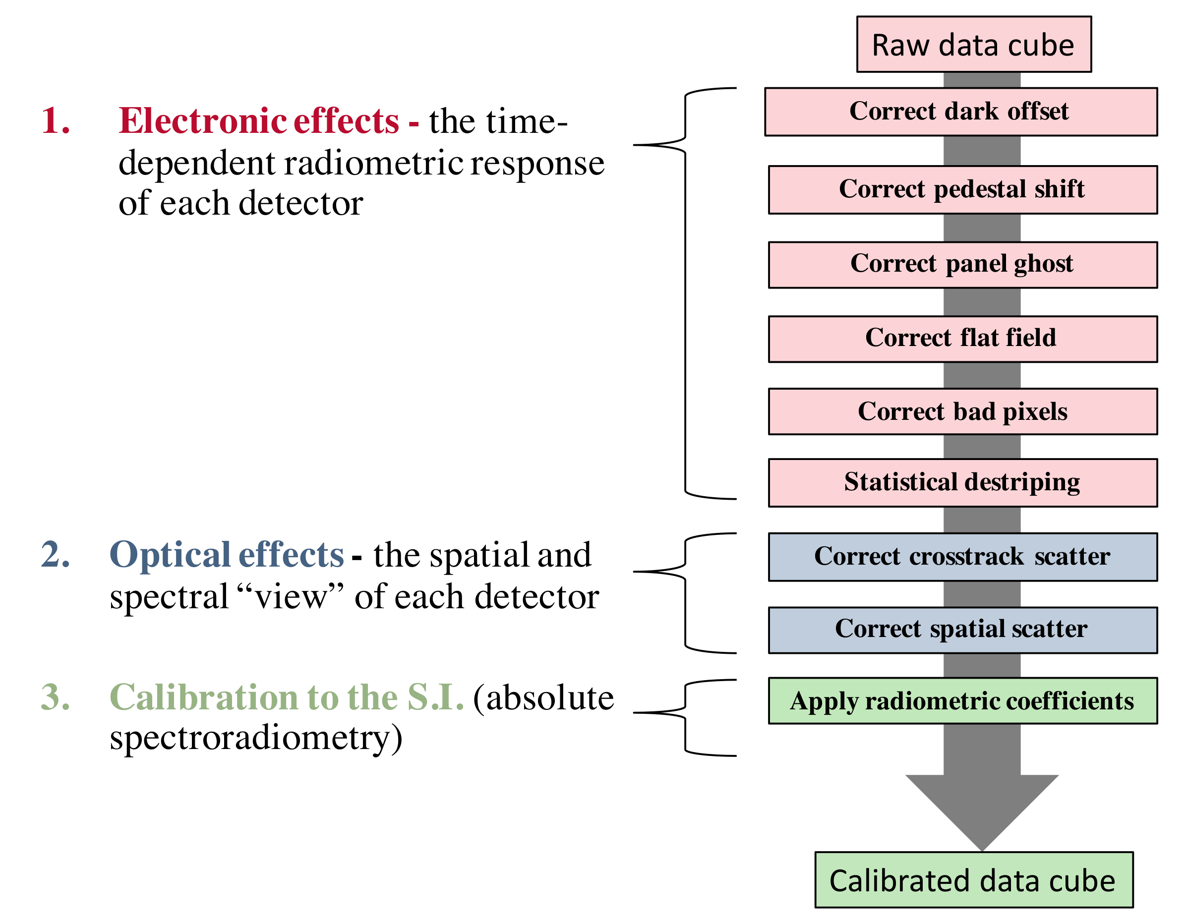
2.1. Algorithmic Approach

Figure 1 illustrates different temporal scales at which various calibration parameters are estimated and the spatial scales of the FPA over which they operate. The intermediate case of the FPA sub-region relates to that portion of the FPA not used in pedestal-shift or stray-light characterization. The temporal scales separate naturally into three regimes comprised of: electronic and thermal effects, which typically change on a per-acquisition or even per-millisecond basis; detector responsiveness and alignment effects, which tend to change on longer timescales such as a thermal cycle or campaign; and optical effects based on the instrument construction which are generally stable after commissioning. In some cases, in-flight methods can validate initial laboratory calibrations estimates of these parameters. In other cases, in-flight characterization can increase calibration accuracy by determining parameters that are difficult to measure in a synthetic laboratory test-bed.

Figure 2 shows the procedure used to correct and calibrate each new raw data cube based on these parameters. Working backwards from the FPA, the calibration steps employed can be divided thematically into sections. First we account for and correct the purely electronic effects of the detector. These include some standard calibration routines, such as correcting for dark current offset, pedestal shift (an overall shift in the dark current), electronic panel ghosting, and flat field correction. In addition, we have employed novel approaches to bad pixel correction and image destriping, described in the sections that follow. Next we account for the optical effects that arise from stray light scattered through interactions with the grating and optical system. One of these optical effects, crosstrack scatter, can reduce spatial contrast and cause halo artifacts to appear around bright high-contrast areas [4]. A related effect, spectral scatter, can reduce contrast in sharp atmospheric features and distort surface reflectances [2]. Finally, we apply radiometric calibration corrections to the raw data cube to obtain absolute spectroradiometry.

Calibration measurements to characterize AVIRIS-NG’s detector responsiveness are taken at beginning of each flight campaign, though additional calibration measurements may also be taken later during particularly long deployments. One such measurement is the flat field response of the instrument, which characterizes the spectral signal of the FPA as a function of spatial position.

The absolute response of the detector is first measured using a NIST-calibrated standard irradiance lamp, which illuminates a Spectralon standard reflectance panel placed in the field of view of the instrument, shown in Figure 3 and Figure 4.

The precision power supply driving the lamp is regularly sent out for factory calibration. The standard lamp and panel used are dedicated to this application and are typically no less than two years old and they incur few hours of use. Because this is an a-priori technique of calibration transfer, adherence to strict geometric dimensions and control of stray, unaccounted-for light sources impinging upon the panel are key. This is achieved with portable rigid fixturing, extreme black-out measures and baffling, and rigorous measurement of stray light for subtraction.

Next the relative response of the FPA is measured using a linear integrating sphere mounted on a swinging track positioned below the instrument at a uniform distance from the FPA, shown in Figure 5, ensuring each spatial pixel receives the same radiance. The absolute response is then scaled to the relative response, producing the calibration flat field image. The integrating sphere moves along a circular arc to ensure that it fills the entire field of view of the instrument, while presenting a similar illumination across the array. While the sphere design homogenizes the spatial illumination, the AVIRIS-NG detector is sensitive enough to measure differences across the aperture that are significant at the sub-percent level. Consequently, we use statistical approaches to select the brightest area of the aperture and track it across the path of the swinging sphere within the instrument field of view.

2.2. Radiometric Calibration

The conversion from DNs to measured radiance uses the linear relationship

$$L_{FPA}(\lambda ,x)=\left[D(\lambda ,x)-\alpha (\lambda ,x)\right]\beta (\lambda ,x),$$

(1)

where $L_{FPA}(\lambda ,x)$ is a function of wavelength $\lambda$ and cross-track spatial location x. The terms $\alpha (\lambda ,x)$ and $\beta (\lambda ,x)$ represent the offset and gain measured in DNs, respectively.

The offset $\alpha (\lambda ,x)$ can be further decomposed into an additive combination

$$\alpha (\lambda ,x)={\alpha }_{dark}(\lambda ,x)+{\alpha }_{ped}\left(x\right),$$

(2)

where ${\alpha }_{dark}(\lambda ,x)$ corresponds to the dark current and ${\alpha }_{ped}\left(x\right)$ corresponds to the pedestal shift. We estimate these parameters using the 1000 lines recorded with the shutter closed at the beginning of each flight-line. The dark current represents changes that arise from the thermal environment of the instrument on timescales of minutes or hours, depending on the length of acquisition. However, the long term temporal reliability of the instrument ensures the dark current level remains stable across multiple flight campaigns. Figure 6 depicts the mean dark current stability over all bands from 2014 through 2018.

An illumination of any region of the FPA will result in an overall shift in the dark current everywhere, known as the pedestal shift. The pedestal shift is characterized independently for each spectrum using the non-illuminated edges of the focal plane, which have been physically masked to ensure no stray light contamination. From this characterization, the pedestal shift is estimated and subtracted from each spectrum independently.

The gain term $\beta (\lambda ,x)$ in Equation (1) is a radiometric calibration coefficient (RCC) and can also be further decomposed into the multiplicative form

$$\beta (\lambda ,x)={\beta }_{RCC}\left(\lambda \right){\beta }_{flat}(\lambda ,x),$$

(3)

where ${\beta }_{RCC}\left(\lambda \right)$ is the spatially independent calibration coefficient and ${\beta }_{flat}(\lambda ,x)$ is the spatially dependent flat field. Here we note that the average flat field value in each spectral channel, that is the average of all cross track positions, is constrained to unity

$$\left[\frac{1}{\left|\chi \right|}\sum _{x\in \chi }{\beta }_{flat}(\lambda ,x)\right]=1\forall \lambda .$$

(4)

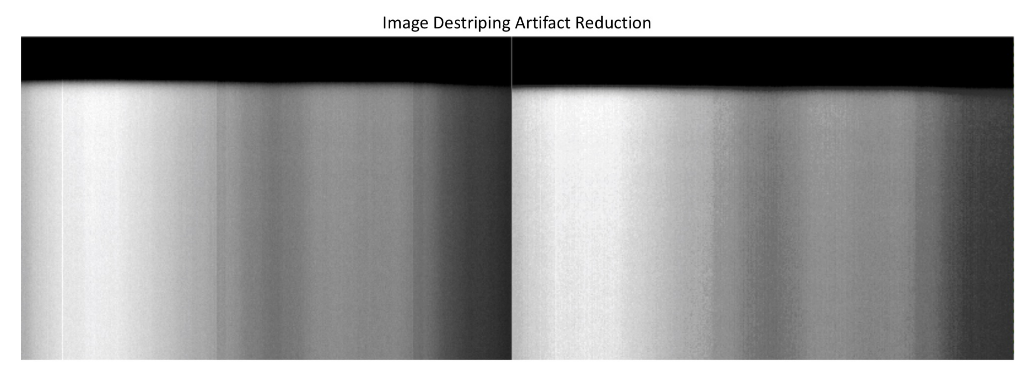
2.3. Markov Field Destriping

Pushbroom imaging spectrometer data can often exhibit transient systematic distortions that manifest as striping artifacts due to variations in detector response. These effects are generally below the 1% level but can be cosmetically significant for downstream data products derived with sensitive retrieval algorithms. An optional destriping procedure employed for AVIRIS-NG utilizes a flight-line-specific correction based on the spatially smooth OnBoard Calibrator (OBC). The OBC provides stimulus at multiple illumination levels. The illumination is not perfectly uniform, as (for example) a flat field acquisition, but it is locally smooth across the detector field of view which reveals fine-scale discrepancies among focal plane array elements.

We use this local spatial smoothness in our destriping model, positing that neighboring detectors’ responses should be similar. We use a simple linear transformation to relate an undistorted measured radiance $L^{\prime }$ to an initial measured radiance $L_M$. The process begins by defining the image correction as:

$$L^{\prime }(\lambda ,x)=\alpha (\lambda ,x)L_M(\lambda ,x)+\beta (\lambda ,x),$$

(5)

where, x corresponds to the indexes of the spectral image. The correction is independent of channel, so we omit the $\lambda$ parameter from subsequent notation. $\alpha \left(x\right)$ represents the focal plane array (FPA) element gain and $\beta \left(x\right)$ represents the FPA element offset. Next we define a cost function:

$$\begin{array}{cc}\hfill f(\alpha ,\beta )=& {\psi }_0\sum _{r,x^{\prime }}{\left[L_M\left(x\right)-L_M(x+1)\right]}^2\hfill \\ \hfill & +{\psi }_1\sum _{x^{\prime }}{\left[\alpha \left(x\right)-1\right]}^2+{\psi }_2\sum _{x^{\prime }}{\left[\beta \left(x\right)\right]}^2\hfill \end{array}$$

where the three coefficients ${\psi }_0$, ${\psi }_1$, and ${\psi }_2$ weight the three error term’s contributions. The first term penalizes horizontal discontinuities in OnBoard Calibrator (OBC) segments, the second term holds $\alpha$ near unity, and the last term holds $\beta$ near zero. This approach is statistically equivalent to minimizing the posterior log likelihood of a Markov Random Field with Gaussian edge potentials and a prior on correction coefficients.

We perform this optimization once per flight to determine the corrections for $\alpha$ and $\beta$, which are both matrix valued variables with one element per pixel on the FPA array. While this results in over ${10}^6$ free parameters, the optimization is manageable using gradient descent techniques. The details of this calculation appear in Appendix A. During an actual campaign, we use very conservative settings for error terms ${\psi }_0$, ${\psi }_1$, and ${\psi }_2$, strongly favoring the original observation to ensure that the destriping does not distort real features of the spectra.

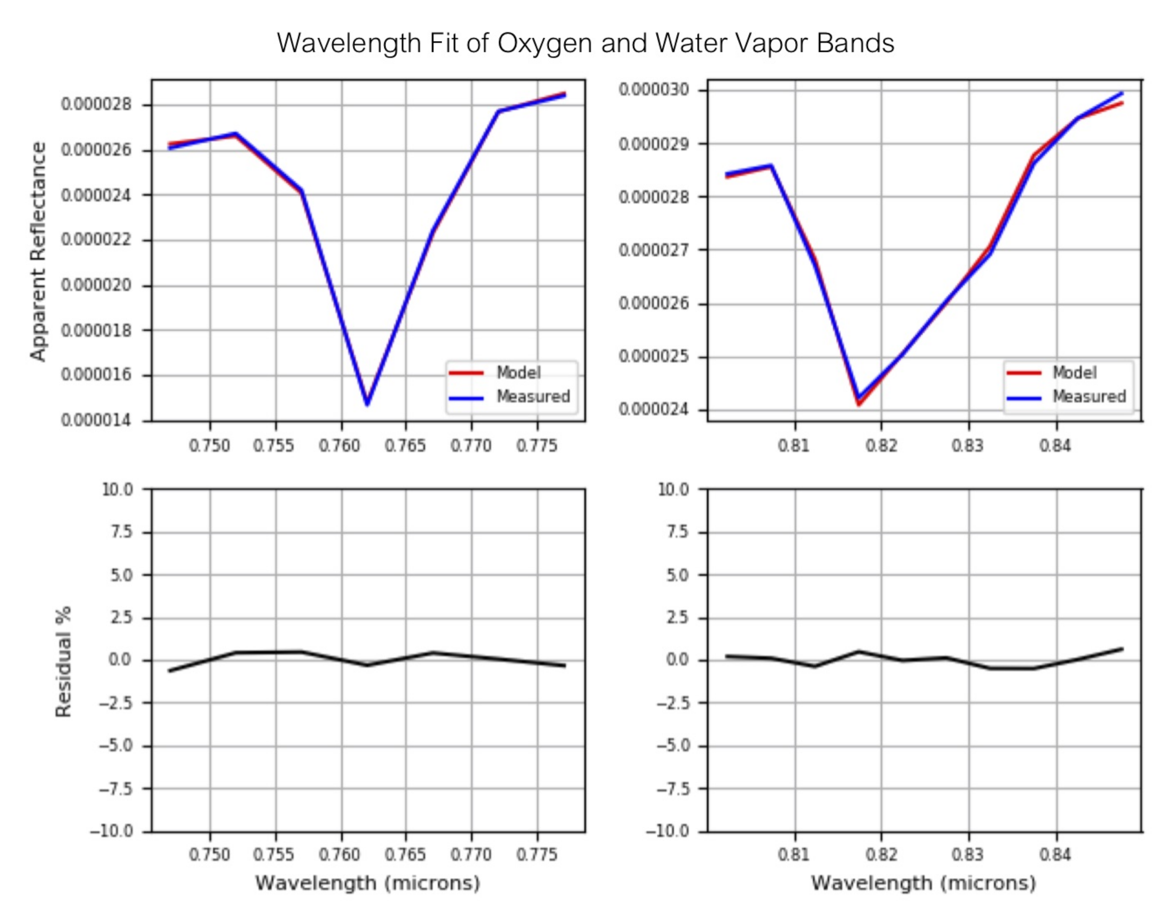
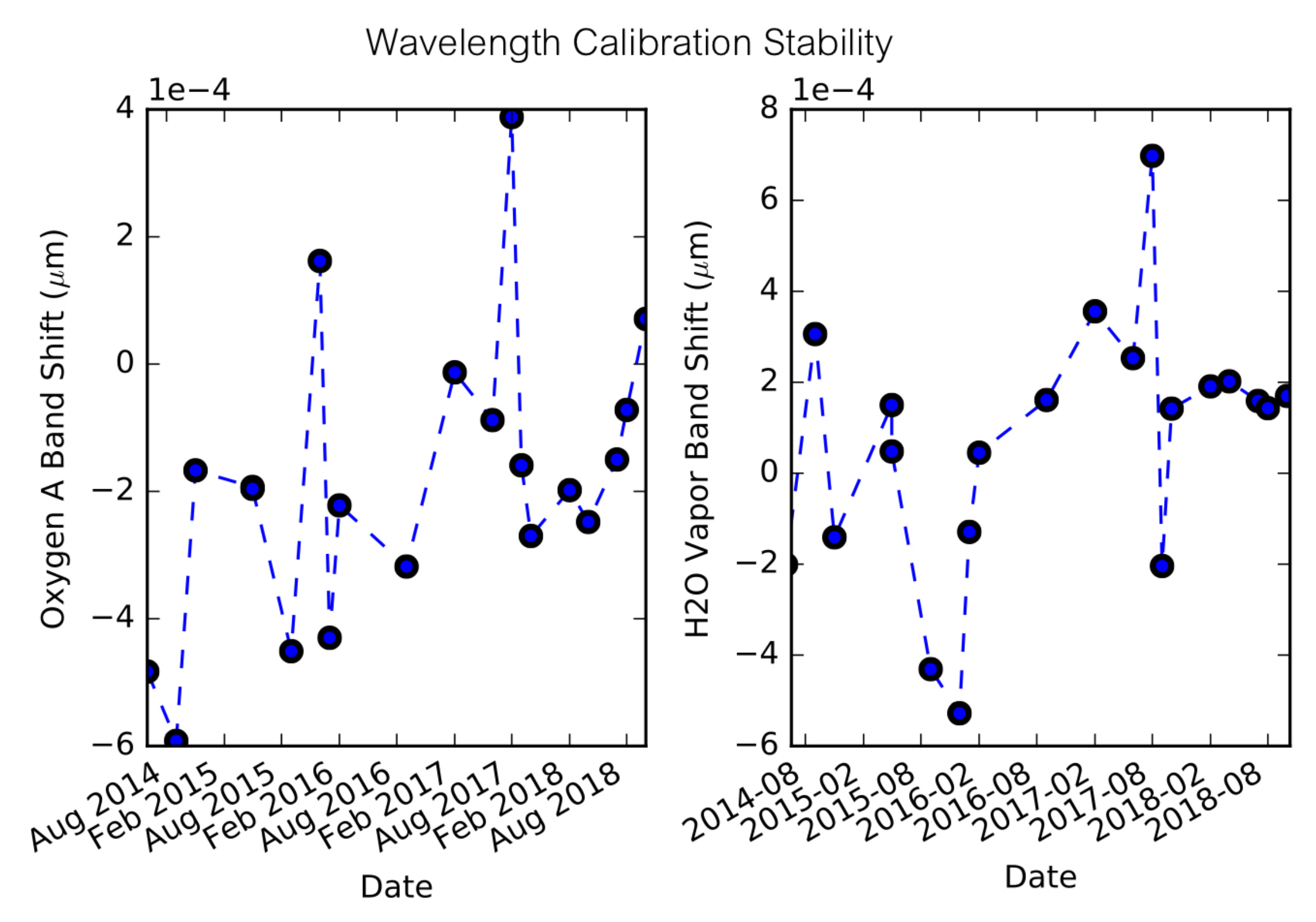
2.4. Atmospheric Wavelength Calibration

The wavelength calibration procedure begins with an initial laboratory spectral calibration. An Action SpectraPro 500i monochromator fed by a broad-band quartz-halogen lamp is used to produce a scanning narrow band laser source (∼1 nm) to characterize the nominal response function center wavelengths and full width half maximum (FWHM) of the detector array. The initial wavelength calibration is derived for six stimuli at 406.7 nm, 532 nm, 632.8 nm, 1064 nm, 1551 nm, and 2064 nm [2].

We refine the initial wavelength calibration with flight data using a single uniform shift to match atmospheric absorption features in the top of atmosphere (TOA) reflectance spectrum. The basic procedure is described by Thompson et al. [5] but we reproduce it here for completeness. The features of the TOA reflectance spectrum $\rho$ are formed from the radiance measurement $L_M$ at wavelength $\lambda$, after normalizing for extra-terrestrial solar irradiance F and solar zenith $\theta$:

$$\rho \left(\lambda \right)=\frac{\pi L_M\left(\lambda \right)}{F\left(\lambda \right)cos\left(\theta \right)}$$

(6)

We model the TOA spectrum as a locally-linear continuum attenuated by gaseous absorption of the 760 nm oxygen band and the 820 nm water vapor band. The spectral attenuation is governed by a Beer-Lambert law based on the gas absorption coefficient $\kappa \left(\lambda \right)$ obtained from a 20 layer model atmosphere:

$$\widehat{\rho }\left(c\right)=h\left({\varphi }_1\right)\left[{\varphi }_2{e}^{}-{\varphi }_3\kappa ({\varphi }_4+\lambda )+{\varphi }_5({\varphi }_4+\lambda )\right],$$

(7)

where ${\varphi }_i$ is the free parameter optimized by the fitting procedure. The function $h\left({\varphi }_1\right)$ is the convolution with a Gaussian Spectral Response Function (SRF) with a FWHM given by ${\varphi }_1$. ${\varphi }_2$ is the local continuum level at 100%, and ${\varphi }_3$ represents the absorption path length. ${\varphi }_4$ represents the wavelength shift, the parameter we sought to recover, and the local continuum slope is represented by ${\varphi }_5$. We fit these parameters using a Nelder-Mead simplex algorithm [6].

2.5. Statistical Bad Pixel Replacement

The AVIRIS-NG focal plane array, like most detectors, contains isolated pixels or clusters of pixels with a response that differs significantly from their neighbors. Some do not respond at all. While the number of these bad pixels is small—less than 0.1% of the total—the single-channel artifacts they create are a significant contaminant since they create outlier spectra that are obvious in data statistics and derived products. We identify these bad pixels at commissioning through the traditional method of using a flat field measurement produced with a uniformly illuminated spatially-uniform calibration object, such as an integration sphere. We flag outlier pixels manually by thresholding their standard deviations. The resulting bad pixel list has remained stable since commissioning.

While bad pixels are only cataloged once, they must be corrected independently in each image frame using a statistically appropriate method of interpolating pixel values for bad elements. Simple interpolation in the spectral dimension is inadequate, since it does not respect the channel-wise structure of real spectra; it distorts the underlying data statistics which must remain pristine for downstream analyses. Instead, we make use of the spectral shapes of nearby locations that are similar to the spectrum undergoing correction. Given a spectrum $s^{\prime }$ with bad pixels, we identify the most similar spectrum in its image frame, $s^{*}$, and then fit a linear relationship between the radiance values of $s^{*}$ and $s^{\prime }$. Similarity between spectra is defined by the spectral angle

$${\mathbf{s}}^{*}=argmi{n}_s\frac{\langle {\mathbf{s}}^{\prime },\mathbf{s}\rangle }{\left|\right|{\mathbf{s}}^{\prime }{\left|\right|}^2{\left|\right|\mathbf{s}\left|\right|}^2}.$$

(8)

After identifying $s^{*}$, we predict the missing values in the incomplete spectrum by fitting a regression model that maps spectral points of $s^{*}$ onto the incomplete spectrum $s^{\prime }$, minimizing least squares error with standard closed-form expression. Naturally, we exclude the bad channels from this calculation. We then apply the map to predict the missing values in $s^{\prime }$.

2.6. Scene Invariances as Point Spread Function Calibration Standards

The measured radiance $L_M\left(\lambda \right)$ represents the best estimate of light at the detector, using the nominal Gaussian line shape first measured in the laboratory. However, any physical instrument exhibits some degree of non-Gaussian response behavior. These perturbations often take the form of “thick tails” to the response function; even at levels which are three or four orders of magnitude below the peak, they can reduce the spectral contrast of features such as sharp atmospheric absorptions [2]. Such distortions arise because, in practice, each incoming ray is partially scattered through interactions with different areas of the optical system and the scattered light ultimately propagates onto multiple areas of the detector array. These unwanted signals cause spatial and spectral blurring within the scene. The effects may be difficult to characterize in the laboratory because (a) high-contrast calibration stimuli may not provide sufficient illumination to measure the non-Gaussian response without also creating pathological detector readout electronic effects or saturation; and (b) it is difficult to replicate the complete, spatially-extended ray bundle any detector element observes in flight conditions. As a result, our characterization and correction of the point spread function’s extended non-Gaussian response relies heavily on flight data.

2.7. Response Function Model

Once the standard radiometric calibrations are performed along with the absolute wavelength determination, we estimate the stray spectral response function as described in [2]. We define a matrix representing the incoming at-aperture radiance for a large number of wavelengths d, where $d\gg 480$, at each of the 640 cross-track locations, ${\mathbf{L}}_A$. The Gaussian nominal SRF is represented by the linear operator $\mathbf{H}$ of size $480\times d$. A vertical stack of single SRF per output channel was used in order to transform the at-aperture radiance, ${\mathbf{L}}_A$, into the nominal instrument output ${\mathbf{L}}_N=\mathbf{H}{\mathbf{L}}_A$. Due to the fact that the matrix $\mathbf{H}$ has a rank less than d, the nominal SRF was not invertible and it eliminated spectral details finer than the instrument’s ideal resolution. The resultant nominal response ${\mathbf{L}}_N$ contained dimensions of a data frame, a $480\times 640$ matrix with 480 spectral channels and 640 cross-track positions.

The measured response ${\mathbf{L}}_M$ was calculated by distorting the nominal response ${\mathbf{L}}_N$ by the stray spectral response, modeled as a $480\times 480$ linear operator $\mathbf{G}$. In addition, a small Gaussian random variable $ϵ$ is added, which combines the read noise, dark noise, and photon shot noise in quadrature. This allowed for the following operations:

$$\begin{array}{c}\hfill \begin{array}{cc}\hfill {\mathbf{L}}_M=& \mathbf{G}\mathbf{H}{\mathbf{L}}_A+\mathbf{H}{\mathbf{L}}_A+ϵ\hfill \\ \hfill {\mathbf{L}}_M=& \mathbf{G}{\mathbf{L}}_N+{\mathbf{L}}_N+ϵ\hfill \\ \hfill {\mathbf{L}}_M=& [\mathbf{G}+\mathbf{I}]{\mathbf{L}}_N+ϵ\hfill \\ \hfill {\mathbf{L}}_M=& \mathbf{A}{\mathbf{L}}_N+ϵ\hfill \end{array}\end{array}$$

(9)

where $\mathbf{A}$ corresponds to the stray spectral response operator with an identity matrix added along it’s diagonal, as performed in prior work by [7]. The correction operator allowed us to recover the nominal data frame which would have been found under the nominal spectral response function by inversion of the stray spectral response functions influence. The Moore-Penrose pseudoinverse ${\mathbf{A}}^{+}={\left({\mathbf{A}}^T\mathbf{A}\right)}^{-1}{\mathbf{A}}^T$ was calculated guaranteeing ${\mathbf{A}}^{+}\mathbf{A}=\mathbf{I}$. The resulting most probable unperturbed measurement $\widehat{{\mathbf{L}}_N}$ was then:

$$\widehat{{\mathbf{L}}_N}={\mathbf{A}}^{+}{\mathbf{L}}_M$$

(10)

Because the AVIRIS-NG instrument is a pushbroom spectrometer, the SRF contains both spatial and spectral support. This type of function is still capable of representing critical shapes, such as axis-aligned multivariate Gaussians, and they have been shown effective in modeling stray SRF observed on different instruments [8]. In the description that follows, we treat the response function as decomposable into independent 1-dimensional operations in the spatial and spectral regime. This family of functions includes the Gaussian distribution.

Estimating SRF from Flight Data

Our SRF estimation builds on previous radiance matching approaches [9,10,11] and is described in [2]. We use the Oxygen A band, located at 760 nm, due to its sharp feature that changes predictably under differing viewing geometries. The band is also largely free of interference from other absorbing gasses and its wavelength location is far from the most damaging aerosol and Rayleigh scattering effects.

The absorption feature of the A band is proportional to the integrated air pressure along the path from the sun to the ground to the sensor, referred here as pressure altitude, while the shape of the feature itself provides leverage in estimating several SRF parameters. Each element of the SRF is defined as

$$\mathbf{A}(i,j)=\frac{1}{z_j}\left[\left(\alpha \right)e^{-{(i-j)}^2/{\sigma }^2}+(1-\alpha )I_{i=j}\right],$$

(11)

where i and j correspond to the rows and columns of the SRF matrix. The normalization constant $z_i$ enforced a row sum of unity and $I_{i=j}$ is the identity matrix. The parameters $\alpha$, which controls the relative magnitude of the SRF and the nominal SRF, and $\sigma$, which is the standard deviation of the SRF, are free parameters optimized during the fit.

We apply the candidate SRF corrections to the nominal radiance $L_T$ spectra and compared the results to the predicted radiance using the error score

$$E(\alpha ,\sigma )=\left|\right|{\mathbf{L}}_{corr}-{\mathbf{L}}_N{\left|\right|}_{O_2},$$

(12)

where $\left|\right|·{\left|\right|}_{O_2}$ is the RMS error taken over the region of the FPA in an envelope four channels wide about the A band.

2.8. Geometric Processing

Geometric processing is the final step applied to the radiometrically and spectrally calibrated AVIRIS-NG image data. The geometric processing system used to generate orthocorrected AVIRIS-NG products is an extension the system developed for processing AVIRIS (classic) data [12]. The AVIRIS-NG data collection system uses an onboard C-MIGITS III GPS/INS system to recover the position (x, y, altitude) and orientation (pitch, roll, true heading) of AVIRIS-NG as a function of scan line. The CMIGITS position and orientation data is used to map a photogrammetric camera model to the current providing pointing vectors for each of the 640 across-track elements in the AVIRIS-NG detector array by accounting for the aircraft velocity and the 100 Hz AVIRIS-NG scan rate. We compute surface coordinates for each pixel by tracing rays cast from each detector element to the surface, represented by a georeferenced Digital Elevation Model. The majority of AVIRIS-NG orthocorrected products are geocoded with respect to 1-arcsecond (30 m/pixel) SRTM DEM, preferring void filled products for flightlines in the continental US. Surface geocoding errors for both low and high altitude scenes are typically on the subpixel scale, and larger localization errors typically result from inaccuracies in the DEM caused by spatial aliasing or missing data.

The AVIRIS-NG orthoprocessing system incorporates several upgrades not implemented in the AVIRIS classic system. The primary change to the existing orthoprocessing system are streaming capabilities, permitting real time geolocalization as new scan lines are saved to disk. Rather than geocoding an entire flightline after acquisition completes, scan lines are stored in a rolling memory buffer and iteratively saved to disk. This functionality required new routines to estimate the average pixel size and downtrack binning factors using a short buffer of initial frames. To exploit the improved spatial resolution of the AVIRIS-NG sensor, surface coordinates are computed via bilinear interpolation among the DEM pixels adjacent to the surface intersection point of the ray traced from each detector elements. A subset of the DEM centered on the the initial aircraft position for the current flightline is cached in memory on initialization to speed up ray to surface intersection tests.

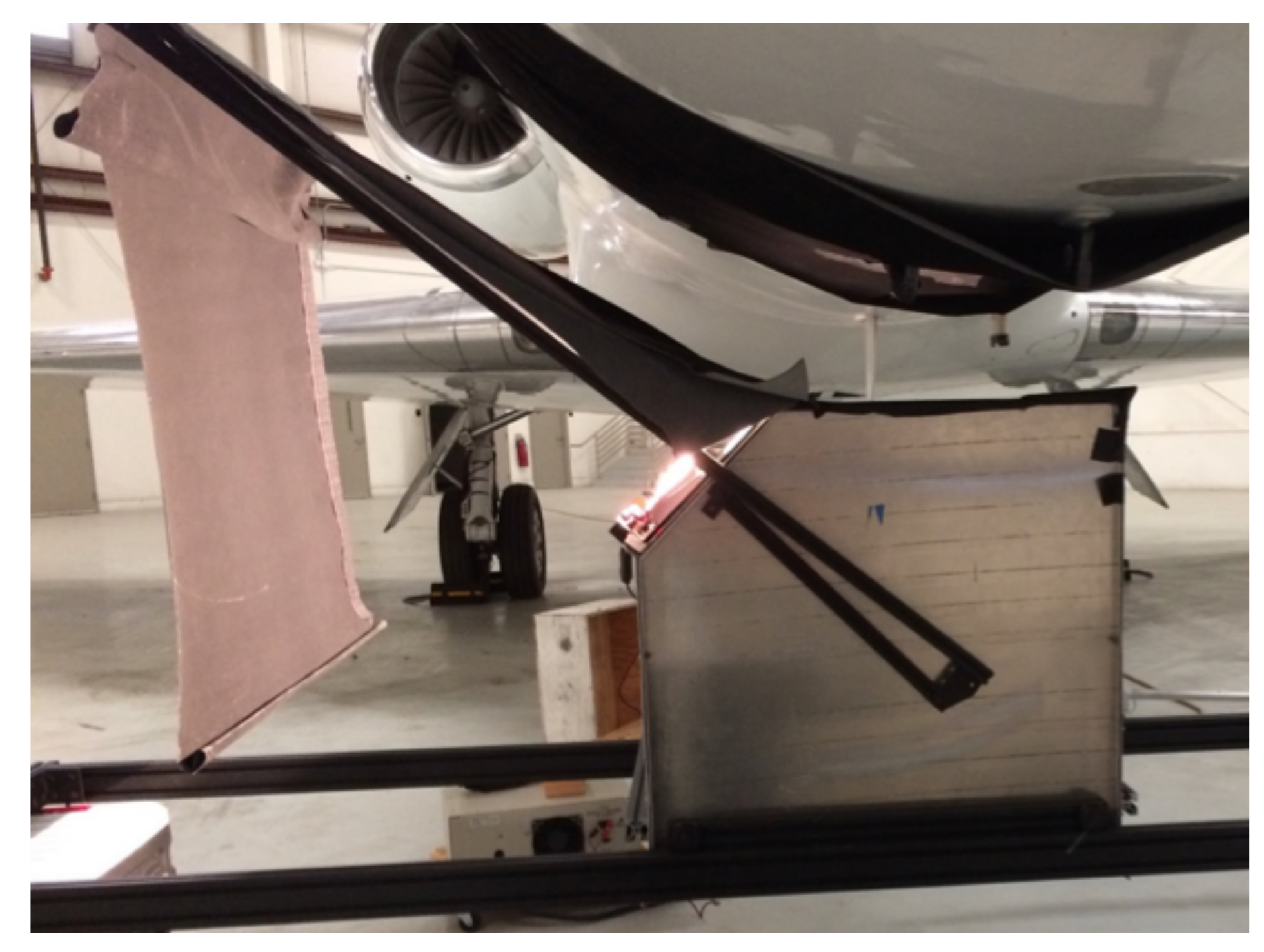
2.9. Laboratory and Field Protocols

The SRF estimation was performed using a single AVIRIS-NG 2014 spectral and radiometric data acquisition over Death Valley National Park, California. This overflight was determined to be optimal because of the large elevation gradient within the scene, spanning more than 3000 m from Telescope Peak to Badwater basin, allowing for an exploitation of variable pressure altitudes and A band depths. The Death Valley acquisition also was largely free of haze contamination and vegetation, limiting unwanted stray absorptions [2].

The AVIRIS-NG data acquisition accuracy was evaluated using both remote and in situ measurements of Ivanpah Playa, NV. This location was chosen due to its uniformity and lack of vegetation, as well as having been found to have minimal aerosol influence. A ground team measured the in situ reflectance, following the protocols described in [5,13] and, using the ratio of surface to reference measurements, compared the absolute reflectance measurements to remote airborne retrievals[2]. The fit best suited for the PSF was determined to be Gaussian using a direct comparison between laboratory measurements using a tunable laser and the atmospheric model fit [2].

2.10. Evaluation on Historical Data

An analysis of the flight data from the Death Valley transect confirmed the Gaussian shape produced the best match of those distributions examined (Pareto, Lorentz, Voigt, and Gaussian), with a mean squared error of 0.1032 [2]. Similarly, the PSF correction to the SRF performed well in minimizing the difference between the top of atmosphere reflectance spectra, demonstrating that the model is capable of correcting an observed mismatch between nominal and measured spectra. The successful PSF correction is further illustrated by the reduction of the pressure altitude bias observed between the retrieved and actual pressure altitude measurements within the Death Valley transect. An analysis of the Ivanpah Playa scene revealed the PSF correction reduced the error from 577 m to 75 m, highlighting the invariance of the model correction across different scenes.

3. Results

3.1. Flat Field Calibration

The temporal stability of the flat field calibration procedure is extremely important not only to the fidelity of downstream products such as radiance, but also in allowing for accurate comparisons of time-series flights over the same targets. Figure 7 illustrates the relative root mean square (RMS) of each flat field used in AVIRIS-NG calibration from 2014 through 2018. Here we note that the flat field procedure was further improved during the beginning of 2017 flight season to more accurately sample FPA response of the illuminated panel. The procedural change improves stability of the instrument’s flat field standard by an order of magnitude.

3.2. Radiometric Calibration

Similar to the flat field stability, the downstream data product uniformity is very sensitive to the spatially independent radiometric calibration coefficients’ temporal stability. The calibration coefficients are calculated at the beginning of each flight campaign using the swinging integration sphere and NIST-calibrated lamp, shown in Figure 3, Figure 4 and Figure 5. Figure 8 shows the dispersion of RCC measurements cross all spectral channels for those calibrations used between 2014 and 2018 flight season.

The standardization of the AVIRIS-NG radiometric calibration procedure has resulted in the calculated radiometric calibration coefficients differing by only a factor 1.4% between the flight seasons sampled, with the largest change occurring between October 2015 and May 2018 of only 2.3%. Changes in the standard deviation of the calibration coefficients across calibration instances is stable to within a factor of ${10}^{-5}$. The decreased variance over the most recent instances, between March 2017 and July 2018, shows an increased stability by an order of magnitude as compared to the flight seasons sampled, further pointing to the continued improvement of the standardization of the procedure.

3.3. Image Destriping

The focal plane array element discrepancies, modeled using the OBC’s spatially smooth behavior, are minimized using cost function analysis leveraging a gradient descent approach. The resulting imagery shows a reduction in the striping artifact that can distort downsteam data products. Figure 9 shows the results of the correction applied to an image sample of the OBC transition region.

The left panel shows the uncorrected boundary between the dark collect and first illumination level of the OBC’s transition region. The vertical striping artifacts are enhanced by the non-uniform OBC illumination panel, highlighting the fine-scale differences between focal plane array elements. Applying the flight-line-specific destriping correction in many cases greatly reduces these fine-scale focal plane array discrepancies resulting in a smoother cross-track pixel uniformity, shown on the right panel.

3.4. Wavelength Calibration

The results of the wavelength shifts are shown in Figure 10. Here we have found that the model matches the measured spectrum with a residual error less than $1\%$, placing it within the limits of the spectrometer’s radiometric accuracy. A historical analysis of atmospheric wavelength shift as compared to the model TOA spectrum from a sample of flights between 2014 through 2018 is shown in Figure 11, illustrating the long term accuracy of the calibration procedure. The AVIRIS-NG instrument design, which uses a triple-blaze convex grating, almost entirely eliminates the appearance of imaging artifacts such as the spectral smile or spatial keystone, which are common amongst imaging spectrometers. This design makes it possible to achieve spatial and spectral uniformity greater than 97% while maintaining high SNR. The empirical calibration procedure is an independent check of cross-track spectral uniformity. Applying the Nelder-Mead procedure to different cross-track locations resulted in an average shift of less than 0.1 nm, or 2% of the FWHM across the image field of view [13].

4. Discussions

The authors are aware of other procedures and instrumentation used to spectrally and radiometrically characterize and calibrate various Electro-optical (EO) sensor designs, however, the procedures evolved for AVIRIS-NG have not been compared to other approaches. Rather, the results of these efforts have been effectively compared and tested against the requirements of product generation, including radiative transfer models, and used to validate the fundamental calibration of other programs, including LANDSAT [14], GOES 16 [15] and MASTER [16].

Procedures optimized for the radiometric and spectral calibration of AVIRIS-NG sensor are unique. They have evolved over years of consistent effort to hone techniques and improve overall certainty, guided by quantitative feedback in regards to data product accuracy. For example, calibration best practices state that a calibration source most optimally stimulate the Device Under Test (DUT) to approximately half its dynamic range [17]. The use of 3000 K halogen lamps as sources for instrument responses optimized for 6000 K sunlight poses a particular challenge. Steps have been taken to ensure sufficient blue light exists without excessive amounts of NIR occurring in our sources. Along these lines, spectral bandpass determination using a halogen pumped monochromator can be problematic in the blue, which why a tunable laser source is used for AVIRIS-NG spectral characterization. Another example of calibration procedure evolution and departure from industry standard practices is the use of the swinging sphere approach to flat-fielding, rather than a single semi-uniform source.

Other EO sensor calibration approaches the authors are aware of include radiative transfer techniques, where a stable spectro-radiometer is used to transfer the known radiance of the lamp-illuminated panel to a source (typically an integrating sphere) placed in the FOV of the DUT [18,19]. The stability of the transfer radiometer, the source, and the transfer methodology are all extra contributors to the compound error buildup. The technique of viewing the calibrated source directly with the DUT avoids these possible errors. Another EO sensor calibration approach involves the use not of calibrated sources (halogen lamps of known irradiance), but of inherently calibrated spectro-radiometer detectors of an a-priori known absolute response utilizing trapped quantum efficient detectors, which are used to put a calibration on a source for the DUT [20]. This method has yet to be thoroughly tested and accepted as an economical replacement for source-based calibration techniques.

The latest calibration validation methods being applied to AVIRIS-NG data involve in-scene cues [2]. So far they have been in close agreement to expectations, in part due to the accuracy of the fundamental calibration of AVIRIS NG. This assertion, however, is beyond the scope of this paper, and will be discussed in future publications.

Future Directions

Work on improving parameter estimation and radiance calculation has already begun in earnest with several potential algorithmic schemes being explored. One such avenue involves leveraging optimal estimation (EO) algorithms [21] to constrain parameter estimates to a much greater degree. The utilization of EO allows for a more robust uncertainty analysis and the use of Bayesian priors, due to its intrinsically probabilistic formalism. Another promising direction being explored for future work proposes the use of digital-pixel FPAs [22] in place of traditional FPAs. One of the major advantages of the digital FPAs is that they perform in-pixel signal digitization, which allows them to have much higher dynamic range and SNR capability.

5. Conclusions

The algorithmic approach of calibration procedures in conjunction with laboratory analysis and historical validation employed in this analysis has been shown to greatly reduce calibration parameter uncertainties as well as the prevalence of image artifacts. These disparate approaches coupled with the overall temporal stability of the instrument ensure optimal downstream image product processing, capable of coherent time series scientific analysis. The flat fielding and radiometric calibration procedure applied across the 2014 to 2018 flight seasons results in low relative variability, with marked improvements in stability over the 2017 and 2018 flight seasons. Image striping artifacts, often harmful to downstream image data products, are noticeably reduced using a pre-computed cost function analysis. Atmospheric wavelength corrections, calculated using the top of atmosphere model spectrum at the 760 nm oxygen A band and the 820 nm water vapor band, are shown to be with the limits of the AVIRIS-NG spectrometer’s radiometric accuracy, and a historic analysis of the corrections exhibits extremely low variability over the 2014 to 2018 flight seasons.

References

1. Thompson, D.R.; Guanter, L.; Berk, A.; Gao, B.C.; Richter, R.; Schläpfer, D.; Thome, K.J. Retrieval of Atmospheric Parameters and Surface Reflectance from Visible and Shortwave Infrared Imaging Spectroscopy Data. Surv. Geophys. 2018, 40, 333–360. [Google Scholar] [CrossRef] [Green Version]
2. Thompson, D.R.; Boardman, J.W.; Eastwood, M.L.; Green, R.O.; Haag, J.M.; Mouroulis, P.; Van Gorp, B. Imaging spectrometer stray spectral response: In-flight characterization, correction, and validation. Remote. Sens. Environ. 2018, 204, 850–860. [Google Scholar] [CrossRef]
3. Green, R.O.; Eastwood, M.L.; Sarture, C.M.; Chrien, T.G.; Aronsson, M.; Chippendale, B.J.; Faust, J.A.; Pavri, B.E.; Chovit, C.J.; Solis, M.; et al. Imaging Spectroscopy and the Airborne Visible/Infrared Imaging Spectrometer (AVIRIS). Remote. Sens. Environ. 1998, 65, 227–248. [Google Scholar] [CrossRef]
4. Mouroulis, P.; Green, R.O.; Van Gorp, B.; Moore, L.B.; Wilson, D.W.; Bender, H.A. Landsat swath imaging spectrometer design. Opt. Eng. 2016, 55, 015104. [Google Scholar] [CrossRef]
5. Thompson, D.R.; Gao, B.C.; Green, R.O.; Roberts, D.A.; Dennison, P.E.; Lundeen, S.R. Atmospheric correction for global mapping spectroscopy: ATREM advances for the HyspIRI preparatory campaign. Remote. Sens. Environ. 2015, 167, 64–77. [Google Scholar] [CrossRef]
6. Nelder, J.A.; Mead, R. A Simplex Method for Function Minimization. Comput. J. 1965, 7, 308–313. [Google Scholar] [CrossRef]
7. Zong, Y.; Brown, S.W.; Johnson, B.C.; Lykke, K.R.; Ohno, Y. Simple spectral stray light correction method for array spectroradiometers. Appl. Opt. 2006, 45, 1111–1119. [Google Scholar] [CrossRef] [PubMed]
8. Haag, J.M.; Van Gorp, B.E.; Mouroulis, P.; Thompson, D.R. Radiometric and spectral stray light correction for the portable remote imaging spectrometer (PRISM) coastal ocean sensor. In Proceedings of the Earth Observing Systems XXII, San Diego, CA, USA, 6–10 August 2017; SPIE: Bellingham, WA, USA, 2017; Volume 10402, p. 104020E. [Google Scholar] [CrossRef]
9. Guanter, L.; Segl, K.; Sang, B.; Alonso, L.; Kaufmann, H.; Moreno, J. Scene-based spectral calibration assessment of high spectral resolution imaging spectrometers. Opt. Express 2009, 17, 11594–11606. [Google Scholar] [CrossRef] [PubMed] [Green Version]
10. Kuhlmann, G.; Hueni, A.; Damm, A.; Brunner, D. An Algorithm for In-Flight Spectral Calibration of Imaging Spectrometers. Remote. Sens. 2016, 8, 1017. [Google Scholar] [CrossRef]
11. Richter, R.; Schlapfer, D.; Muller, A. Operational Atmospheric Correction for Imaging Spectrometers Accounting for the Smile Effect. IEEE Trans. Geosci. Remote. Sens. 2011, 49, 1772–1780. [Google Scholar] [CrossRef]
12. Boardman, J.W. Precision geocoding of low altitude AVIRIS data: Lessons learned in 1998. In eAVIRIS 1999 Proceedings; Jet Propulsion Laboratory: La Cañada Flintridge, CA, USA, 1999; pp. 63–68. [Google Scholar]
13. Thompson, D.R.; Leifer, I.; Bovensmann, H.; Eastwood, M.; Fladeland, M.; Frankenberg, C.; Gerilowski, K.; Green, R.O.; Kratwurst, S.; Krings, T.; et al. Real-time remote detection and measurement for airborne imaging spectroscopy: A case study with methane. Atmos. Meas. Tech. 2015, 8, 4383–4397. [Google Scholar] [CrossRef]
14. Chander, G.; Markham, B. Revised landsat-5 tm radiometric calibration procedures and postcalibration dynamic ranges. IEEE Trans. Geosci. Remote. Sens. 2003, 41, 2674–2677. [Google Scholar] [CrossRef] [Green Version]
15. Czapla-Myers, J.S.; Anderson, N.J. Post-Launch Radiometric Validation of the GOES-16 Advanced Baseline Imager (ABI). In Society of Photo-Optical Instrumentation Engineers (SPIE) Conference Series; SPIE: Bellingham, WA, USA, 2018; Volume 10785, p. 107851F. [Google Scholar] [CrossRef]
16. Hook, S.J.; Myers, J.J.; Thome, K.J.; Fitzgerald, M.; Kahle, A.B. The MODIS/ASTER airborne simulator (MASTER) a new instrument for earth science studies. Remote. Sens. Environ. 2001, 76, 93–102. [Google Scholar] [CrossRef]
17. Jablonski, J.; Durell, C.; Slonecker, T.; Wong, K.; Simon, B.; Eichelberger, A.; Osterberg, J. Best Practices in Passive Remote Sensing VNIR Hyperspectral System Hardware Calibrations. In Hyperspectral Imaging Sensors: Innovative Applications and Sensor Standards 2016; SPIE: Bellingham, WA, USA, 2016; Volume 9860, p. 986004. [Google Scholar] [CrossRef]
18. Guanter, L.; Kaufmann, H.; Segl, K.; Foerster, S.; Rogass, C.; Chabrillat, S.; Kuester, T.; Hollstein, A.; Rossner, G.; Chlebek, C.; et al. The EnMAP Spaceborne Imaging Spectroscopy Mission for Earth Observation. Remote. Sens. 2015, 7, 8830–8857. [Google Scholar] [CrossRef] [Green Version]
19. Baumgartner, A.; Gege, P.; Köhler, C.; Lenhard, K.; Schwarzmaier, T. Characterisation methods for the hyperspectral sensor HySpex at DLR’s calibration home base. In Proceedings of the Sensors, Systems, and Next-Generation Satellites XVI, Edinburgh, UK, 24–27 September 2012; International Society for Optics and Photonics: Bellingham, WA, USA, 2012; Volume 8533, p. 85331H. [Google Scholar]
20. Fox, N.P. Trap Detectors and their Properties. Metrologia 1991, 28, 197–202. [Google Scholar] [CrossRef]
21. Rodgers, C.D. Inverse Methods for Atmospheric Sounding: Theory and Practice; World Scientific Publishing Co.: Singapore, 2000. [Google Scholar]
22. Schultz, K.; Kelly, M.W.; Blackwell, M.H.; Brown, M.G.; Colonero, C.B. Digital-pixel focal plane array technology. Linc. Lab. J. 2014, 20, 36–51. [Google Scholar]
Figure 1. Spatial scales over which calibration parameters operate (vertical axis) and the temporal scales over which they typically change (horizontal axis).
Remotesensing 11 02129 g001
Figure 2. Sequence of steps used for calibrating a cube of raw AVIRIS-NG data.
Remotesensing 11 02129 g002
Figure 3. Apophotic box deployment for hanger calibration. The interior is lined with 2% black polishing cloth. On the top face of the box, there is an aperture enabling a view of the standard panel inside. A frame similar to arrangement on left controls lamp and panel geometry. Note curtain preventing reflected lamp light from illuminating the panel inside the box. For this (less portable) methodology, no background measurement is necessary.
Remotesensing 11 02129 g003
Figure 4. Lamp-and-panel frame with shutter deployment for hanger calibration. Shutter is deployed with lamp on. Data is then acquired for measurement of background illumination. Note entrance slit aperture of AVIRIS-NG at in aircraft belly at top of photo. This particular hangar cal was performed in the sub-tropics. The fan is to keep insects off of the lamp.
Remotesensing 11 02129 g004
Figure 5. Linear integrating sphere on swinging track below the mounted AVIRIS-NG instrument in the flight hanger.
Remotesensing 11 02129 g005
Figure 6. Dark current stability of AVIRIS-NG across all bands. The flight data used spans multiple different campaigns across North America, Greenland, Europe, and India from June 2014 through October 2018. The mean dark currents were calculated by taking the mean across all spectral channels for each sample flight after determining the lack of dark current variability between individual channels. The mean and standard deviation of the sampled flight data is 5.984 × 10 6 and 5.676 × 10 6 , respectively.
Remotesensing 11 02129 g006
Figure 7. Flat field stability as a function of time. The RMS for each calibration flat field image (blue) shows the dynamics of the signal relative to the signal mean. The standard deviation of the Flat field RMS measurements for the population of flat fields prior to 2017 (left) is R M S σ 2.1 × 10 3 whereas the population of flat fields post 2017 Flat field RMS standard deviation (right) is R M S σ 2.6 × 10 4 .
Remotesensing 11 02129 g007
Figure 8. Measurement stability of AVIRIS-NG calibration coefficients across all spectral channels from 2014 to 2018. The decreasing variance of the line profile in recent years is indicative of an increasing uniformity of pre and post-flight campaign calibration procedures.
Remotesensing 11 02129 g008
Figure 9. Destriping method comparison between the uncorrected OBC transition region (left) and a correction fitting both FPA offset and gain (right) from Equation (5).
Remotesensing 11 02129 g009
Figure 10. Wavelength calibration model and empirical fit comparisons to the 760 nm oxygen band (left) and 820 nm water vapor band (right). In these regions, the model match the measured spectrum with a residual error that is within the limits of the AVIRIS-NG spectrometer’s radiometric accuracy.
Remotesensing 11 02129 g010
Figure 11. Atmospheric wavelength calibration shift over time of the 760 nm and 820 nm spectral bands as measured against the most recent (2018) AVIRIS-NG wavelength calibration baseline. The flight data sampled spans multiple campaigns across North America, Greenland, Europe, and India from June 2014 through October 2018.
Remotesensing 11 02129 g011