Ship Detection in Optical Satellite Images via Directional Bounding Boxes Based on Ship Center and Orientation Prediction

Abstract

To accurately detect ships of arbitrary orientation in optical remote sensing images, we propose a two-stage CNN-based ship-detection method based on the ship center and orientation prediction. Center region prediction network and ship orientation classification network are constructed to generate rotated region proposals, and then we can predict rotated bounding boxes from rotated region proposals to locate arbitrary-oriented ships more accurately. The two networks share the same deconvolutional layers to perform semantic segmentation for the prediction of center regions and orientations of ships, respectively. They can provide the potential center points of the ships helping to determine the more confident locations of the region proposals, as well as the ship orientation information, which is beneficial to the more reliable predetermination of rotated region proposals. Classification and regression are then performed for the final ship localization. Compared with other typical object detection methods for natural images and ship-detection methods, our method can more accurately detect multiple ships in the high-resolution remote sensing image, irrespective of the ship orientations and a situation in which the ships are docked very closely. Experiments have demonstrated the promising improvement of ship-detection performance.

1. Introduction

Ship detection in remote sensing imagery has attracted the attention of many researchers due to its wide applications such as maritime surveillance, vessel traffic services, and naval warfare. Although many methods have shown promising results [1,2,3], ship detection in optical remote sensing images with complex backgrounds is still challenging.

The optical remote sensing images are often contaminated by mists, clouds, and ocean waves, resulting in the low contrast and blurring of the ship targets. In complex scene, the background on the land would have similar textures and colors with the inshore ships. Moreover, unlike many objects in natural images, the ships in remote sensing images are relatively small and less clear. They are in narrow-rectangle shapes, with the orientation of arbitrary angles in the image, and usually docked very closely, making it difficult to detect each single ship separately.

Recently, convolutional neural networks (CNN)-based object detection methods for natural images have achieved great improvement in terms of detection accuracy and running efficiency [4,5,6,7]. These methods typically predict horizontal bounding boxes from horizontal region proposals (or anchors) to locate objects, since the objects in natural images are usually placed in horizontal or near-horizontal. Generally, the horizontal box and region proposal are described as a rectangle with 4 tuples $\left(x,y,h,w\right)$, in which $\left(x,y\right)$ denotes the center location of the rectangle, and h, w are height and width, respectively. However, using the horizontal box is very difficult to accurately locate arbitrary-oriented ships in the remote sensing images [8,9,10,11]. Consequently, many CNN-based ship-detection methods are proposed to predict rotated bounding boxes from rotated region proposals [8,9,10]. The rotated box and region proposal are usually described as a rotated rectangle with 5 tuples $\left(x,y,h,w,\theta \right)$, in which the additional variable $\theta$ denotes the orientation (or angle) of the rotated box.

Many object detection methods for natural images [5,6] and ship-detection methods [8,10] usually use each pixel in the feature map as the center location $\left(x,y\right)$ to generate region proposals. However, objects in remote sensing images usually only occupy a small portion of the images. This results in many useless region proposals at the locations without the objects. In addition, the feature map is usually generated with substantial downsampling, e.g., 1/16 in [5] as compared to original image. Although all pixels of the feature map are used to generate region proposals, they are still sparse compared to the resolution of original image. This is unfavorable for detection of small objects, because there might be no pixel or only a few pixels on the feature map right locating on the objects.

On each center location $\left(x,y\right)$, the rotated region proposals are usually generated by predefining some fixed angles of orientation ($\theta$), scales ($\sqrt{hw}$), and aspect ratios ($h:w$) [8,10]. 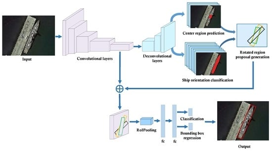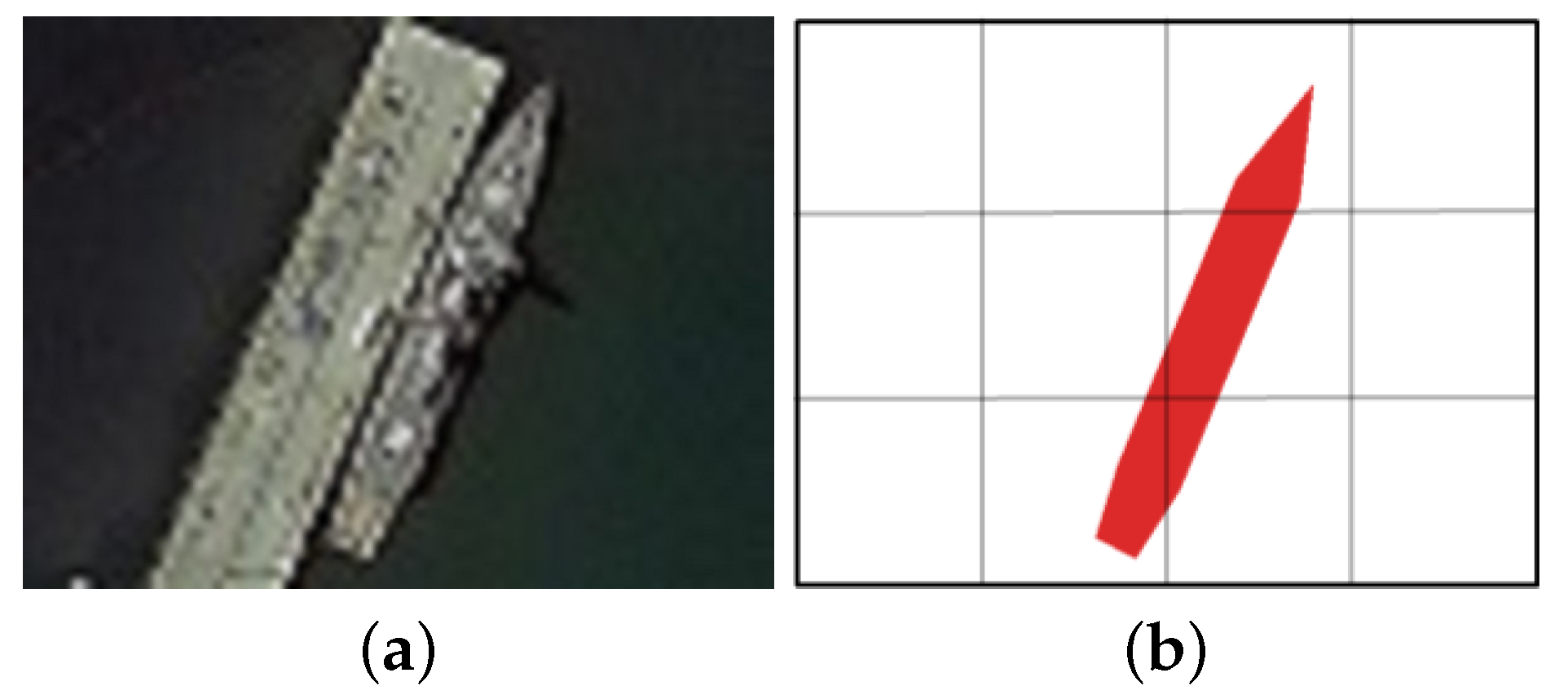Predefining some fixed values of scales and aspect ratios can be fine for horizontal region proposal generation, which has been proved in many object detection methods (e.g., Faster R-CNN [5], SSD [6], YOLOv3 [12]). However, predefining some fixed values for the angles may not be a good choice. Since ships are usually in narrow-rectangle shapes, the Intersection-over-Union (IoU) overlap between the region proposal and the ground-truth box is very sensitive to the angle variation of the region proposal. As shown in Figure 1, in (a), when the angle difference between the region proposal (red box) and the ground-truth box (yellow box) is for example ${7.5}^{\circ }$, the IoU overlap is 0.61. However, in (c), when the angle difference increases to ${30}^{\circ }$, the IoU overlap drops to 0.15. Under such small IoU, it is very difficult for CNN to accurately predict the ground-truth box from the region proposal. Furthermore, the angle of the rotated region proposal can span a large range (i.e., ${180}^{\circ }$). Hence, a relatively large number of fixed values need to be preset for the angle (for example, 6 values are set for the angle in ship-detection methods [8,10]), so as to reduce the angle difference, making the prediction from the region proposal to the ground-truth box easier. However, this would generate massive region proposals, leading to the increase of computational cost. In this case, we usually need to sample a relatively smaller number of region proposals from them for the following detection. This process, however, would unavoidably discard some relatively accurate region proposals, leading to the decrease of detection accuracy.

In this paper, we design center region prediction network to solve the problem caused by using each pixel in the feature map as the center location, and ship orientation classification network to avoid the problem caused by setting many coarse fixed values for the angle of orientation. Center region prediction network predicts whether each pixel in the image is in center region of the ship, and then the pixels in the center region are sampled to determine the center locations of region proposals. In this way, the number of generated region proposals can be greatly reduced and most of them are ensured to be located on the ship. To this end, we introduce per-pixel semantic segmentation into center region prediction network. Ship orientation classification network first predicts a rough angle range of orientation for each ship, and then several angles with higher accuracy can be defined among this range. This only needs a small number of predefined angles. The angle difference between the region proposal and the ground-truth box can also be limited to a smaller value, making the prediction from the region proposal to the ground-truth box easier.

To make the whole detection network simpler and more efficient, ship orientation classification network also performs semantic segmentation via sharing the convolutional features with center region prediction network. In this way, the ship orientation classification network yields nearly free computational cost, yet significantly increases detection accuracy. Moreover, since we do not need to predict very accuracy segmentation results for the center region and the angle range, it is unnecessary to construct very complex semantic segmentation network architecture. We only simply add several deconvolutional layers on the base convolutional layers to perform semantic segmentation for the two networks. By taking advantage of these two networks, a smaller number of rotated region proposals with higher accuracy can be generated. Then, each rotated region proposal is simultaneously classified and regressed to locate the ships in optical remote sensing images.

The rest of this paper is organized as follows. In Section 2, we introduce the related work. Section 3 describes the details of our accurate ship-detection method. In Section 4, experimental results and comparisons are given to verify the superiority of our ship-detection method. Section 5 analyzes the ship-detection network in detail. We conclude this paper in Section 6.

2. Related Work

Ship detection in optical remote sensing images with complex backgrounds has become a popular topic of research. In the past few years, many researchers use hand-designed features to perform ship detection. Lin et al. [13] use line segment feature to detect the shape of the ship. The ship contour feature is extracted in [14,15,16] to perform contour matching. Yang et al. [17] first extract candidate regions using a saliency segmentation framework, and then a structure-LBP (local binary pattern) feature that characterizes the inherent topology structure of the ship is applied to discriminate true ship targets. In addition, the ship head feature served as an important feature for ship detection is also usually used [18,19,20,21]. It is worth noting that it is very hard to design effective features to address various complex backgrounds in optical remote sensing images.

In recent years, CNN-based object detection methods for natural images have achieved great improvement since R-CNN [22] is proposed. These methods can be typically classified into two categories: two-stage detection methods and one-stage detection methods. The two-stage detection methods (R-CNN [22], Fast R-CNN [4], Faster R-CNN [5]) first generate some horizontal region proposals using selective search [23], region proposal network [5] or other sophisticated region proposal generation methods [24,25,26,27]. Then, the generated region proposals are classified as one of the foreground classes or the background, and regressed to accurately locate the object in the second stage. The two-stage methods are able to robustly and accurately locate objects in images and the current state-of-the-art detection performance is usually achieved by this kind of approach [28]. In contrast, one-stage detection methods directly produce some default horizontal region proposals or locate the location of the object, which no longer needs the above region proposal methods. For example, SSD (single shot multibox detector) [6] directly sets many default region proposals from multi-scale convolution feature maps. YOLOv3 (you only look once) [12] divides a single image into multiple grids, and sets five default region proposals for each grid, and then directly classifies and refines these default region proposals. Compared with two-stage detection methods, one-stage methods are simpler and faster, but the detection accuracy is usually inferior to that of two-stage methods [6].

Inspired by CNN-based object detection methods for natural images, many CNN-based ship-detection methods are proposed to perform accurate ship detection in remote sensing images. Unlike the general object detection methods for natural images, the ship detection needs to predict the rotated bounding box to accurately locate ships and avoid missing out the ships docked very closely. Since two-stage detection methods usually produce more accurate object detection results, the researchers pay more attention to this kind of methods. For instance, inspired by R-CNN [22], S-CNN [29] first generates rotated region proposals with line segment and salient map, and then CNN is used to classify these region proposals as ships or backgrounds. Liu et al. [9] detect ships by adopting the framework of two-stage Fast R-CNN [4], in which SRBBS [30] replaces selective search [23] so as to produce rotated region proposals. The above two ship-detection methods achieve better detection performance than the previous methods based on hand-designed features, but they cannot be trained and tested end-to-end, which results in long training and inference time.

Based on Faster R-CNN [5], Yang et al. [10] propose an end-to-end ship-detection network, which effectively uses multi-scale convolutional features and RoI align to more accurately and faster locate ships in remote sensing images. Furthermore, some one-stage ship-detection methods are also proposed. Liu et al. [8] predefine some rotated boxes on the feature map, and then two convolutional layers are added to perform classification and rotated bounding box regression for each predefined box. When the size of the input image is relatively large, this method adopts slide-window strategy to detect multiple small-size images for the detection of the whole image, which greatly increases the detection time. In [11], the coordinates of the rotated bounding boxes are directly predicted based on the detection framework of one-stage YOLO [31]; however, this is quite difficult for CNN to produce accurate prediction results [7].

3. The Proposed Ship-Detection Method

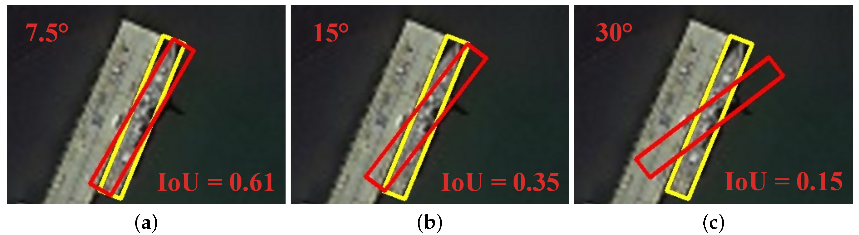
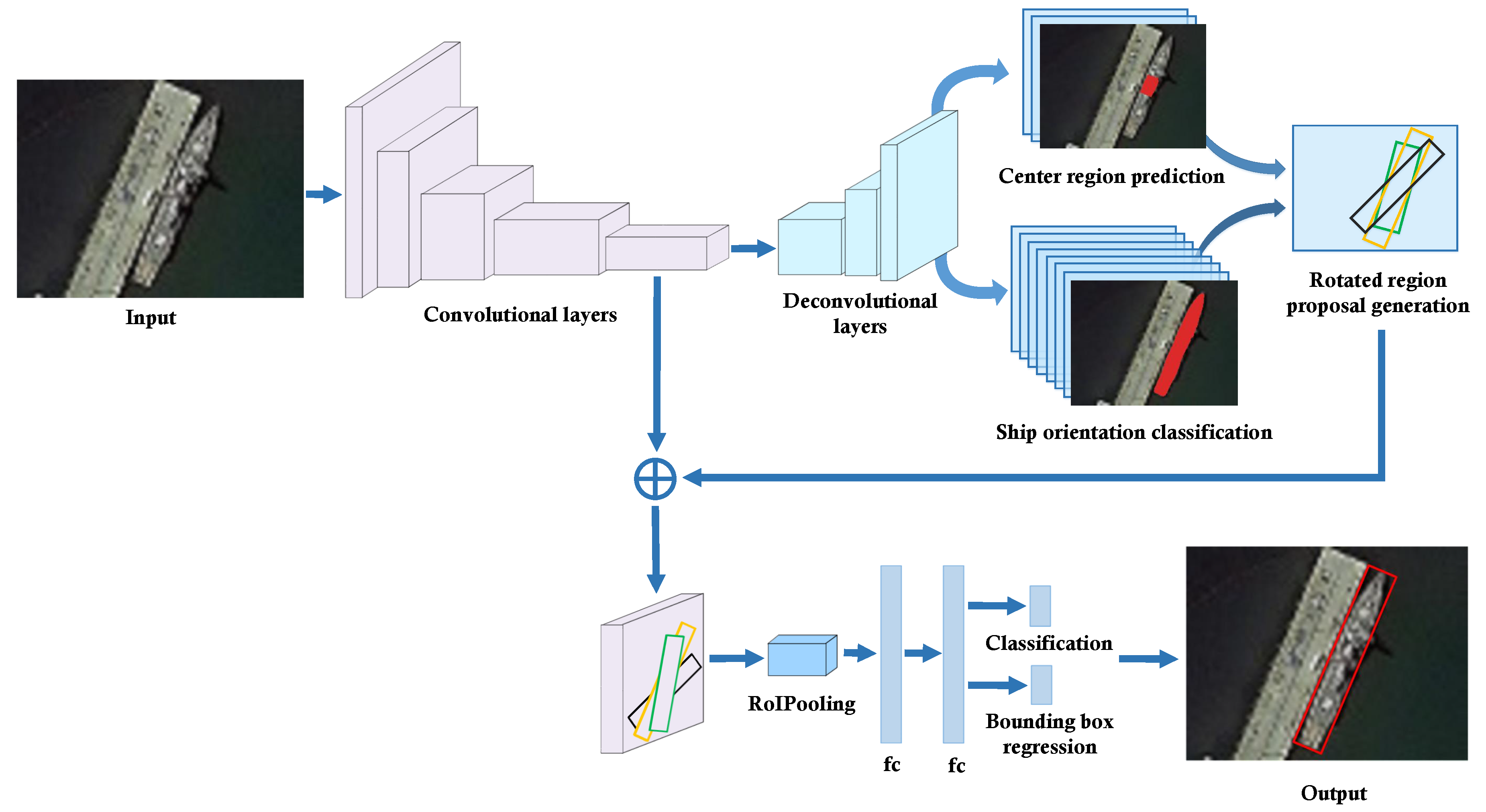
Figure 2 shows the pipeline of the proposed ship-detection method. First, the base convolutional layers are used to extract convolutional features from the input image. Then, unlike the general two-stage object detection methods, we upsample the convolutional features with several deconvolutional layers to perform per-pixel semantic segmentation. This aims to get relatively more accurate center location and orientation of the ship. With such information, more reliable and fewer number of rotated region proposals can be generated, helping to achieve more accurate detection of the ships. As shown in Figure 2, by introducing several deconvolutional layers, center region prediction network and ship orientation classification network are constructed. They share the deconvolutional features with each other, predicting the center region and orientation of the ship, respectively. Based on those two networks, the rotated region proposals with different angles, aspect ratios, and scales are generated. Then, RoI pooling is performed to extract a fixed-size feature representation from the convolutional features of each region proposal. Finally, two fully connected layers (fc) are used to simultaneously perform classification and regression for each region proposal and ultimately generate the refined ship-detection results with rotated bounding boxes.

3.1. Center Region Prediction Network

Faster R-CNN [5] first used each pixel in the feature map to generate region proposals, which effectively combines region proposal generation and bounding box regression into an end-to-end network, producing state-of-the-art detection performance. Since then, many object detection methods [6,32] and ship-detection methods [8,10] adopt this kind of strategy to produce region proposals. However, it might result in two problems in remote sensing images. (1) The sizes of objects in remote sensing images are usually small, only occupying a small portion of the images. In this case, the areas without objects may produce many useless region proposals, which increases the computational load and the risk of false detection in the subsequent stage. (2) The resolutions of the feature maps used to generate region proposals are usually much smaller than those of the input images. For example, in object detection methods [5,33], the resolutions of the feature maps are reduced to 1/16 of those of the input images. There would be no reliable pixel on the feature map to indicate the small objects. This would inevitably degrade the detection performance for small objects. To solve the above problems, the idea of semantic segmentation is incorporated in the detection framework to predict the center region for each object. We can then generate region proposals based on a group of pixels only picked from the center region. In this way, it can avoid blindly generating massive useless region proposals in the region without objects, and let the centers of region proposals could concentrate on the objects regardless of their sizes in the image.

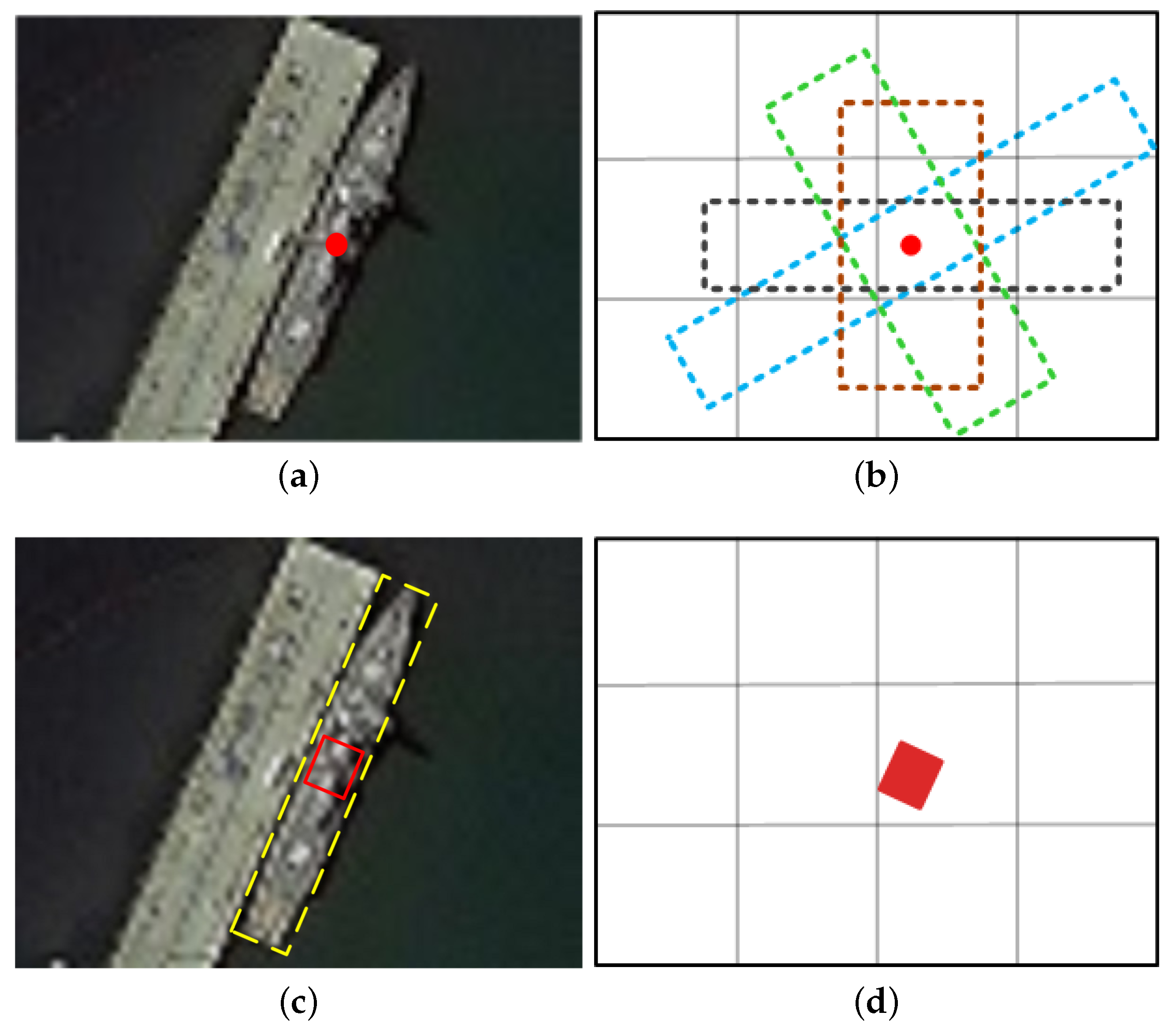
As shown in Figure 3a, for a ship in optical remote sensing image, we first need to predict the center of ship. With the center point $(x,y)$, we can then define a set of rotated region proposals centered at $(x,y)$ with differing angles, aspect ratios, and scales. As shown in Figure 3b, different region proposals share the same center point, which is located on the ship center needing to be predicted. The purpose of defining multiple region proposals on one predicted center point is to get better adaptation for ships with various sizes and shapes.

It is not easy to directly predict the single center point of a ship in the image. As shown in Figure 3c, instead of predicting the exact point of ship center, we change it to predict the center region of ship, i.e., a set of points located at the center of ship (see Figure 3d). Then, a group of pixels sampled from the center region are used to generate region proposals, to increase the probability for accurate ship detection. Another important consideration for predicting the center region rather than the center point is that if only the center point is to be predicted, in the training stage of semantic segmentation, a center pixel for each ship is labeled as positive sample (i.e., 1) in optical remote sensing images, while most of other pixels would be labeled as negative samples (i.e., 0). This would result in a serious class-imbalanced problem. To alleviate this problem, we expand the single point of center to a center region which contains a much larger number of points.

As shown in Figure 3c, the center region is defined as the area labeled by the red box, whose long side is 0.125 of the long side of the ground-truth box (the yellow box in Figure 4c), and short side is 0.75 of the short side of the ground-truth box. We take the pixels in center region as the positive samples (see the red region in Figure 3d), and the pixels in other regions as the negative samples (see the white region in Figure 3d). However, in this way, the number of the positive sample is still small compared with that of the negative sample.

To further compensate for the shortage of the positive sample, we introduce a class-balanced weight to increase the loss of positive samples. This can make the losses of positive samples and negative samples comparable, even if the number of positive samples is smaller than that of negative samples, to avoid class-imbalanced problem. The class-balanced weight $\alpha$ $(\alpha >1)$ is introduced into the following cross-entropy loss function:

$$L_c\left(p,u,v\right)=-\alpha {\displaystyle \sum }_{u\in Y_{+}}log{p}_u-{\displaystyle \sum }_{v\in Y_{-}}log{p}_v,$$

(1)

where $Y_{+}$ and $Y_{-}$ denote the positive sample set and the negative sample set, respectively. $p_u$ denotes the probability that the pixel u is classified as the positive sample. $p_v$ denotes the probability that the pixel v is classified as the negative sample. $p_u$ and $p_v$ are computed with the SoftMax function. $\alpha =\left|Y_{-}\right|/\phantom{\left|Y_{-}\right|\left|Y_{+}\right|}\left|Y_{+}\right|$, where $\left|Y_{+}\right|$ and $\left|Y_{-}\right|$ are the numbers of the positive samples and the negative samples, respectively.

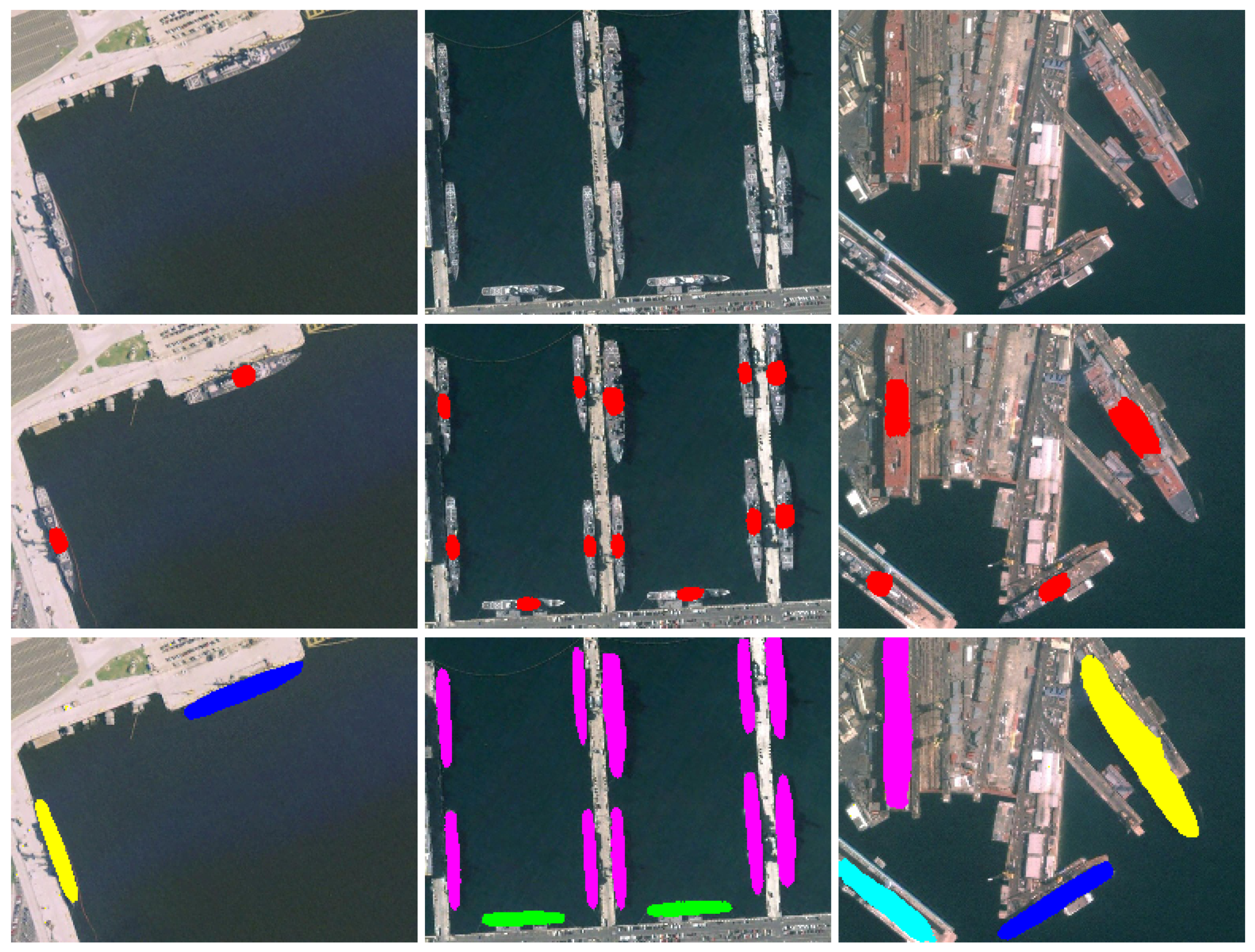
Figure 4 shows some prediction results from center region prediction network. The prediction results are overlaid on input images for better display. The first row shows input images, and the second row shows the prediction results. We can see that the center regions of ships can be properly predicted as expected.

3.2. Ship Orientation Classification Network

The object detection methods for natural images usually generate horizontal region proposals by predefining several fixed scales and aspect ratios in each pixel of the feature map. Inspired by this way, many ship-detection methods [8,10] preset some fixed angles, scales, and aspect ratios to generate rotated region proposals. However, ships in optical remote sensing images are usually in narrow-rectangle shapes, and thus the accuracy of the rotated region proposal is greatly influenced by its orientation angle deviation. A small angle change can drastically reduce the accuracy of rotated region proposal. Thus, it is necessary to predefine more possible angles to improve the accuracy of rotated region proposals. However, the angle of the rotated region proposal spans a very large angle range (i.e., ${180}^{\circ }$), and a large number of angles need to be predefined. This can reduce the interval between two adjacent angles and therefore improve the accuracy of some region proposal, but much more region proposals would be produced, resulting in significant increase of computational cost. In this situation, a smaller number of region proposals usually need to be sampled to increase detection efficiency. However, the sampling operation would inevitably discard some relatively accurate region proposals, causing the decrease of detection accuracy.

To solve this problem, we first predict a rough angle range orientation for each ship in the images. Several possible angles with higher confidence can then be defined among this range. This can limit the angle difference between region proposals and ground-truth boxes to a small value, and only need a limited number of predefined angles. To this end, we construct ship orientation classification network to predict the angle range of the ship. The ship orientation classification network also performs semantic segmentation, which enables it to share the convolutional features with the center region prediction network. In this way, ship orientation classification network yields nearly free computational cost, yet significantly increase detection accuracy.

We fix the whole angle range of orientation to $\left[-{45}^{\circ },{135}^{\circ }\right)$ in this paper. To predict the angle range for each ship in the optical remote sensing images, the whole angle range $\left[-{45}^{\circ },{135}^{\circ }\right)$ is divided into 6 bins (more analysis can be seen in Section 5-B), and each bin is indexed by $i(i=1,2,3,4,5,6)$. As shown in

Table 1. The angles of the rotated region proposals.

Index	Angle Range	Angles of Region Proposals
$i=1$	$\left[-{45}^{\circ },-{15}^{\circ }\right)$	$-{37.5}^{\circ },-{30.0}^{\circ },-{22.5}^{\circ }$
$i=2$	$\left[-{15}^{\circ },{15}^{\circ }\right)$	$-{7.5}^{\circ },{0.0}^{\circ },{7.5}^{\circ }$
$i=3$	$\left[{15}^{\circ },{45}^{\circ }\right)$	${22.5}^{\circ },{30.0}^{\circ },{37.5}^{\circ }$
$i=4$	$\left[{45}^{\circ },{75}^{\circ }\right)$	${52.5}^{\circ },{60.0}^{\circ },{67.5}^{\circ }$
$i=5$	$\left[{75}^{\circ },{105}^{\circ }\right)$	${82.5}^{\circ },{90.0}^{\circ },{97.5}^{\circ }$
$i=6$	$\left[{105}^{\circ },{135}^{\circ }\right)$	${112.5}^{\circ },{120.0}^{\circ },{127.5}^{\circ }$

, the first column lists index i, and the second column lists the angle range of each bin i. Ship orientation classification network performs semantic segmentation and outputs dense per-pixel classification. According to the orientation angle of each ship, the pixels in the ship region are all labeled by a corresponding index i, while the pixels in other locations are labeled as 0. For example, for the remote sensing image shown in Figure 5a, Figure 5b illustrates the ground-truth segmentation label of ship orientation classification network. The orientation angle of the ship is ${67.8}^{\circ }$, and thus the pixels in the ship region are classified as index 4 (denoted with red color), and the pixels in other locations are classified as 0 (denoted with white color). Then, we can define multiple more confident angles for region proposals within the predicted angle range. As a result, the generated region proposals would have smaller number of the angle and higher accuracy.

Similar to center region prediction network, in order to solve the class-imbalanced problem, we define the following class-balanced cross-entropy loss function as

$$L_a\left(p,u,v\right)=-{\displaystyle \sum }_{i=1}^6\left({\beta }_i{\displaystyle \sum }_{u\in Y_i}log{p}_{ui}\right)-{\displaystyle \sum }_{v\in Y_{-}}log{p}_v,$$

(2)

where $Y_i$ denotes the pixel set in ship region indexed by i, and $Y_{-}$ is the pixel set in non-ship region. $p_{ui}$ denotes the probability that the pixel u is classified as the angle index i. $p_v$ denotes the probability that the pixel v is classified as 0. $p_u$ and $p_v$ are computed with the SoftMax function. ${\beta }_i$ denotes the class-balanced weight of each angle index, and we set ${\beta }_i=\left|Y_{-}\right|/\phantom{\left|Y_{-}\right|\left|Y_i\right|}\left|Y_i\right|$, where $\left|Y_i\right|$ and $\left|Y_{-}\right|$ are numbers of $Y_i$ and $Y_{-}$, respectively.

The segmentation results of ship orientation classification network are shown in the third row of Figure 4, in which the ships in different angle ranges are denoted with different colors. We can see that the network can properly predict the angle range of each ship.

3.3. Rotated Region Proposal Generation

In this paper, the region proposal is described as a rotated rectangle with 5 tuples $\left(x,y,h,w,\theta \right)$. The coordinate $\left(x,y\right)$ denotes the center location of the rectangle. The height h and the width w are the short side and the long side of the rectangle, respectively. $\theta$ is the rotated angle of the long side. As mentioned in Section 3.2, $\theta \in \left[-{45}^{\circ },{135}^{\circ }\right)$.

Unlike the objects in natural images, for the ships in remote sensing images, the ratio of width to height can be very large. Thus, we set aspect ratios $(h$:$w)$ of region proposals as 1:4 and 1:8. The scales $\left(\sqrt{hw}\right)$ of region proposals are set as 32, 64, 128, 256. The angles of region proposals are listed in the third column of Table 1. For example, when the orientation angle range of a ship is in $\left[-{15}^{\circ },{15}^{\circ }\right)$, the angles of region proposals are set as $-{7.5}^{\circ },{0.0}^{\circ },{7.5}^{\circ }$. In this case, the angle difference between the region proposal and its ground-truth box will be no more than ${7.5}^{\circ }$. How to set scales, aspect ratios, and angles of region proposals is detailed in Section 5-D.

For a pixel A in the predicted center region of a ship, we can find the pixel B at the same position from the output of ship orientation classification network. Taking the pixel A as the center point of region proposals and the value (the index i) of pixel B to determine the angle range of region proposals, we can generate 3-angle, 2-aspect ratio, and 4-scale region proposals. In an image, the number of pixels in center regions can be very large. Taking all these pixels as the center points of region proposals will generate too many region proposals, which is time-consuming for subsequent operations. To reduce the number of region proposals, for each image, we randomly sample N $(N=100)$ pixels from center regions to generate region proposals (see the more analysis in Section 5-C).

There are a total of 2400 region proposals (100 sampling pixels × 3 angles × 2 aspect ratios × 4 scales) in an image. Some region proposals highly overlap with each other. To reduce redundancy, we adopt non-maximum suppression (NMS) [34]. For NMS, we fix the IoU [11] threshold at 0.7, and the score of each region proposal is set as the probability that the center point of the region proposal is classified as belonging to the center region of a ship. After NMS, per image remains about 400 region proposals.

With center region prediction network and ship orientation classification network, our method only generates 2400 region proposals in an image, which are much fewer than those generated with two-stage representative Faster R-CNN [5]. For an image with size $512\times 384$, Faster R-CNN generates 6912 region proposals with 3 scales and 3 aspect ratios, which are about three times more than those generated with our method. Moreover, experimental results demonstrate that the detection accuracy can be satisfactory with much fewer region proposals.

3.4. Multi-Task Loss for Classification and Bounding Box Regression of Region Proposals

We first assign each region proposal as the positive sample (ship) or the negative sample (background). A region proposal is assigned as the positive sample if its IoU overlap with the ground-truth box is higher than 0.45, and the negative sample if its IoU overlap is lower than 0.45.

The detection network preforms classification and bounding box regression for each region proposal. For classification, the network outputs a discrete probability distribution, $p=\left(p_0,p_1\right)$, over two categories (i.e., ship and background). p is computed with a SoftMax function. For bounding box regression, the network outputs bounding box regression offset, $t=\left(t_x,t_y,t_h,t_w,t_{\theta }\right)$.

We use a multi-task loss to jointly train classification and bounding box regression:

$$L_m\left(p,u,t^{*},t\right)=L_{cls}\left(p,u\right)+u{L}_{reg}\left(t^{*},t\right),$$

(3)

where u indicates the class label ($u=1$ for ship and $u=0$ for background), and $t^{*}$ denotes the ground-truth bounding box regression offset. The classification loss $L_{cls}$ is defined as:

$$L_{cls}\left(p,u\right)=-log{p}_u.$$

(4)

For the bounding box regression loss $L_{reg}$, the term $u{L}_{reg}$ denotes that the regression loss is activated only for the positive sample $(u=1)$ and would be disabled for the negative sample $(u=0)$. We adopt smooth-$L_1$ loss [5] for $L_{reg}$:

$$L_{reg}\left(t^{*},t\right)={\displaystyle \sum }_{i\in \left\{x,y,h,w,\theta \right\}}\mathrm{smoot}{\mathrm{h}}_{L_1}\left(t_i^{*}-t_i\right),$$

(5)

in which

$$\mathrm{smoot}{\mathrm{h}}_{L_1}\left(X\right)=\left\{\begin{array}{cc}0.5X^2\hfill & \mathrm{if}\left|X\right|<1\hfill \\ \left|X\right|-0.5\hfill & \mathrm{otherwise}.\hfill \end{array}\right.$$

(6)

The bounding box regression offsets t and $t^{*}$ are defined as follows:

$$\begin{array}{c}\begin{array}{cc}{t}_x=\left(x-x_a\right)/\phantom{\left(x-x_a\right)w_a}{w}_a,\hfill & t_y=\left(y-y_a\right)/\phantom{\left(y-y_a\right)h_a}{h}_a,\\ t_h=log\left(h/\phantom{h{h}_a}{h}_a\right),\hfill & t_w=log\left(w/\phantom{w{w}_a}{w}_a\right),\end{array}\hfill \\ t_{\theta }=\left(\theta -{\theta }_a\right)\ast \frac{\pi }{180}+k\pi ,\hfill \\ \begin{array}{cc}{t}_x^{*}=\left(x^{*}-x_a\right)/\phantom{\left(x^{*}-x_a\right)w_a}{w}_a,\hfill & t_y^{*}=\left(y^{*}-y_a\right)/\phantom{\left(y^{*}-y_a\right)h_a}{h}_a,\\ t_h^{*}=log\left(h^{*}/\phantom{h^{*}{h}_a}{h}_a\right),\hfill & t_w^{*}=log\left(w^{*}/\phantom{w^{*}{w}_a}{w}_a\right),\end{array}\hfill \\ t_{\theta }^{*}=\left({\theta }^{*}-{\theta }_a\right)\ast \frac{\pi }{180}+k\pi ,\hfill \end{array}$$

(7)

where x, $x_a$ and $x^{*}$ are for the predicted box, region proposal and ground-truth box (likewise for $y,h,w,\theta$), and $k\in Z$ to ensure $t_{\theta },t_{\theta }^{*}\in \left[-\frac{\pi }{4},\frac{3\pi }{4}\right)$.

3.5. End-to-End Training

We define the loss function of the whole detection network as

$$L={\lambda }_c{L}_c+{\lambda }_a{L}_a+{\lambda }_m{L}_m,$$

(8)

where $\left({\lambda }_c,{\lambda }_a,{\lambda }_m\right)$ are balancing parameters. In the training process, $L_c:L_a:L_m$ is about 2:1:1, and thus we set $\left({\lambda }_c,{\lambda }_a,{\lambda }_m\right)$ as (0.5, 1, 1). Our detection network is trained end-to-end using stochastic gradient descent (SGD) optimizer [35]. We use the VGG16 model pre-trained for ImageNet classification [36] to initialize the network while all new layers (not in VGG16) is initialized with Xavier [37]. The weights of the network are updated by using a learning rate of ${10}^{-4}$ for the first 80k iterations, and ${10}^{-5}$ for next 80k iterations. The momentum, the weight decay, and the batch size is set as 0.9, 0.0005 and 2, respectively. Moreover, online hard example mining (OHEM) [38] is adopted to better distinguish ships from complex backgrounds. OHEM can automatically select hard examples to train object detectors, thus leading to better training convergence and higher detection accuracy.

3.6. Network Architecture

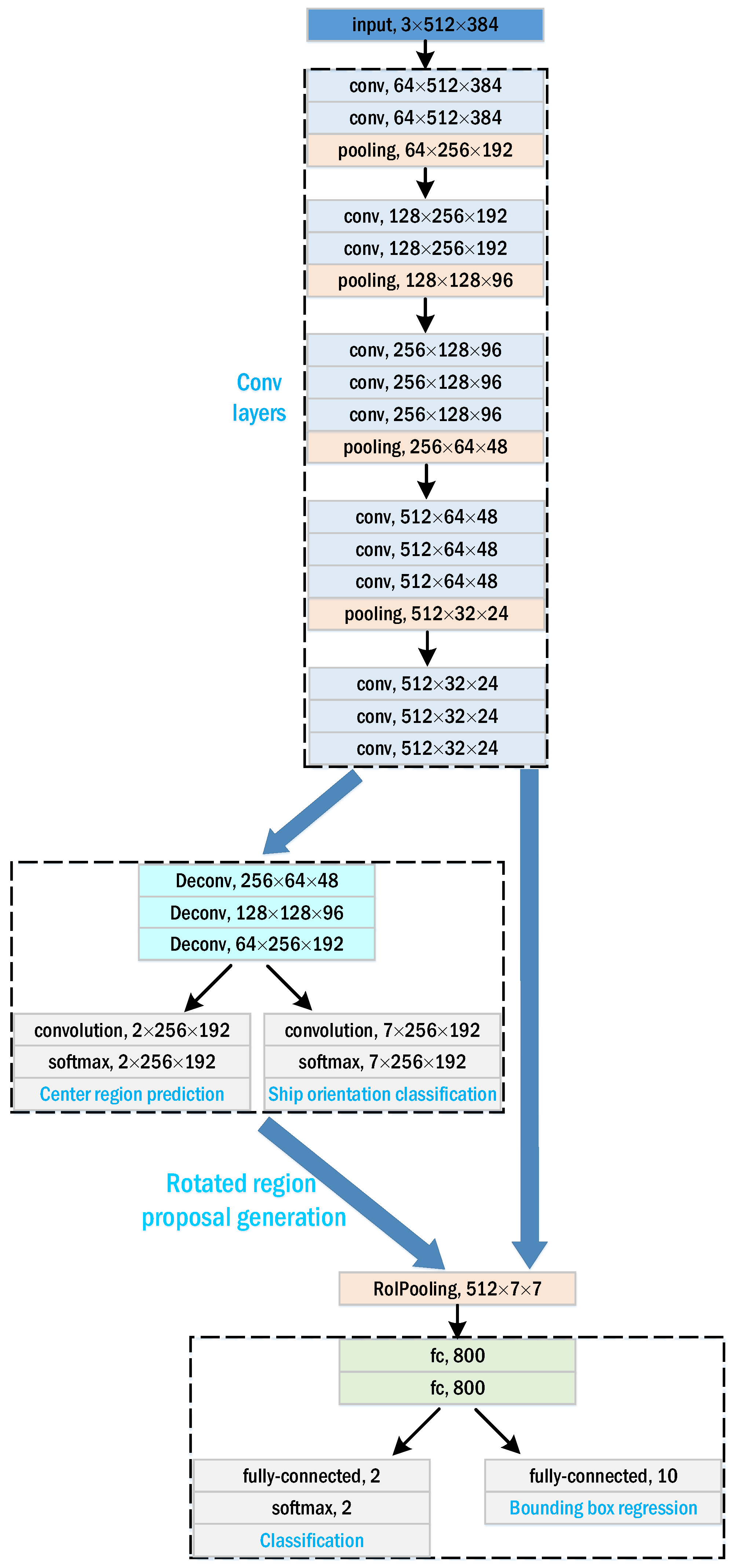
Figure 6 shows the network architecture of our detection network. Details of each part is described as follows:

Input image: the input image is a three-channel optical remote sensing image. The network can be applied on any-size images, but for simplicity, all input images are resized into $3\times 512\times 384$ (channel × width × height).

Conv layers: the 13 convolutional layers in VGG16 model [36] served as the base convolutional layers have been widely used in many applications [5,39,40], and we adopt these 13 convolutional layers to extract image features. As shown in Figure 6, “conv” denotes a convolutional layer followed by a ReLU activation function [41]. The output size of each layer is denoted as channel × width × height (for example, $64\times 512\times 384$). The pooling layer is inserted among the convolutional layers to implement downsampling.

Center region prediction network and ship orientation classification network: the deconvolutional layer is used to upsample feature maps to construct center region prediction network and ship orientation classification network. “Deconv” denotes a deconvolutional layer followed by a ReLU activation function. For speed/accuracy trade-off, the output size for the two networks is set as $256\times 192$ (see the more analysis in Section 5-A).

RoI Pooling: RoI pooling [9,42,43,44] is performed to extract a fixed-size feature representation ($512\times 7\times 7$) from convolutional features for each region proposal, so as to interface with the following fully connected network.

Classification and bounding box regression: Two fully connected layers are used to perform classification and bounding box regression for each region proposal. “fc” in Figure 6 denotes the fully connected layer followed by a ReLU activation function and a dropout layer [45]. “fully connected” denotes the fully connected layer. There are 2 outputs (the probabilities belonging to ship and background) for classification, and 10 outputs (5 offsets for the positive sample and 5 offsets for the negative sample) for bounding box regression.

4. Experiments

4.1. Dataset

In this paper, the data set contains 1599 optical remote sensing images, in which some are collected from Google Earth and some are publicly available [30]. The image resolutions are between 2 m and 0.4 m. The ships in the data set are mainly distributed in the USA (e.g., Norfolk Harbor, San Diego Naval Base, Pearl Harbor, Everett Naval Base, Mayport Naval Base), France (e.g., Toulon), UK (e.g., Plymouth), Japan (e.g., Yokohama), Singapore (e.g., Changi Naval Base).

In the data set, there are more than 25 types of ships with various scales, shapes and angles (see Figure 7a,b). Some images are influenced by clouds, mists and ocean waves (Figure 7c,d). Blurring (Figure 7e), similar color and texture between ships and backgrounds (Figure 7f) also usually exist in these images. Ships can be closely docked side by side (Figure 7g). Moreover, ships can emerge in various contexts, such as shore (Figure 7h), dock (Figure 7i) and sea (Figure 7j). All these factors can increase difficulties for ship detection in optical remote sensing images, and thus it is suitable to evaluate the proposed detection network using our data set.

The data set contains 1599 optical remote sensing images. We randomly select 1244 images as the training set while the remaining 355 images are selected as the testing set. We perform data augmentation to increase the number of training set. Since we aim to detect ships of arbitrary orientation, we augment the data set mainly by rotating the training images with nine angles $({20}^{\circ },{40}^{\circ },{60}^{\circ },{80}^{\circ },{100}^{\circ },{120}^{\circ },{140}^{\circ },{160}^{\circ },{180}^{\circ })$. In addition, three Gaussian functions with different standard deviations (i.e., 1, 2, 3) are used to blur training images. Through data augmentation, we obtain 16,172 training images.

4.2. Implementation Details

For all the convolutional layers in detection network (see Figure 6), the kernel size, the stride and the padding size are set as $3\times 3$, 1 and 1, respectively. In addition, max-pooling with the kernel size $2\times 2$, the stride 2 is adopted. The kernel size, the stride and the padding size of the deconvolutional layer are $4\times 4$, 2 and 1, respectively. We use $10\%$ dropout for the fully connected layer.

We generate 2400 region proposals in an image. After NMS with an IoU threshold of 0.7, there remains about 400 region proposals per image. In the training process, directly classifying all 400 region proposals will introduce class-imbalanced problem, since negative samples dominate in region proposals. To avoid this problem, in the training process, we sample positive and negative samples so that the ratio between them is at 1:3. If there are more than 32 positive samples, we randomly sample 32 positive samples. If the number of positive samples is smaller than 32, we use negative samples to make up 128 region proposals.

In the testing process, all 400 region proposals (if there are more than 400 region proposals, we randomly sample 400 region proposals) are performed classification and bounding box regression. After that, NMS with an IoU threshold of 0.3 is employed to eliminate overlapped boxes, producing the final detection results.

4.3. Comparison

The proposed method is compared with three state-of-the-art CNN-based object detection algorithms for natural images, including Faster R-CNN [5], SSD [6], and YOLOv3 [12]. Faster R-CNN is a two-stage object detection method. The size of the input image of Faster R-CNN is set as $512\times 384$. The scales of region proposals are set as 64, 128, 256 replacing 128, 256, 512 (roughly corresponding to the image of size $1000\times 600$). SSD and YOLOv3 are one-stage object detection methods. For SSD, according to [6], we resize the input image into $512\times 512$. Furthermore, we adopt the default settings for YOLOv3.

Figure 8 shows some ship-detection results in testing data set from Faster R-CNN, SSD, YOLOv3, and the proposed method. Although the testing images in the first row contain very small ships, our method can still produce accurate detection results, while Faster R-CNN and SSD miss out some ships. From the second row to the fourth row, ships and backgrounds are very similar, which is hard for CNN to recognize ships from the background. Faster R-CNN, SSD, and YOLOv3 fail to get good detection results. The images in the fifth row are influenced by mist, causing low contrast. In this situation, the proposed method still gives satisfactory performance, while Faster R-CNN, SSD, and YOLOv3 miss out some ships. For the images in the last four rows, ships are closely docked side by side, which is very common in optical remote sensing images. We can see that the ships docked side by side are accurately detected by our detection network; however, Faster R-CNN, SSD, and YOLOv3 fail to accurately detect these ships.

We also compare our method with three other ship-detection methods, i.e., Method [20], Rotation Dense Feature Pyramid Networks (R-DFPN) [10], Method [46]. Method [20] uses hand-designed features to perform ship detection. R-DFPN [10] and Method [46] are CNN-based ship-detection methods. Some detection results from the four ship-detection methods are shown in Figure 9. In the last column, we can see that our method produces accurate detection results for the six images. Since the hand-designed features-based method [20] cannot design effective features to fit complex backgrounds, in the second column, many ships are missed out. CNN-based R-DFPN also detects ships with rotated bounding boxes. For R-DFPN, the angle of the region proposal is set as some fixed values, causing that the angle difference between the region proposal and the ground-truth box is relatively larger than that of the proposed method. As a result, in the third column, some ships are missed out or inaccurately located. The CNN-based Method [46] first locates the ship heads, and then the region proposals generated with the ship heads are iterative regressed and classified to produce ship-detection results. As shown in the fourth column, since Method [46] uses the horizontal bounding boxes to locate ships, it produces inaccurate location for some ships docked side by side.

We use mean average precision (mAP) and precision and recall curve (P-R curve) to quantitatively evaluate the performances of different detection methods.

Table 2. The mAP for different methods on the testing set.

	Faster R-CNN [5]	SSD  [6]	YOLOv3  [12]	Method [20]	R-DFPN [10]	Method [46]	Ours
mAP	$80.2\%$	$83.6\%$	$86.9\%$	$62.4\%$	$85.7\%$	$84.4\%$	$88.3\%$

gives mAP of different detection methods on the testing set. It can be seen that we produce the highest mAP, outperforming other six detection methods. Figure 10 shows P-R curves of different detection methods. The curves show that our method yields the highest recall, and the largest area under the curve (i.e., mAP). Since YOLOv3 yields the horizontal box to locate the ship, many ships docked side by side are missed out. As a result, our method produces higher recall than YOLOv3, resulting in higher mAP, although the precision of YOLOv3 is slightly higher than that of our method when recall is about in range of [0.75, 0.85].

5. Network Analysis

A. The output sizes of center region prediction network and ship orientation classification network. The output sizes of the two networks can influence the detection accuracy and the running efficiency. Some small ships just take up a small part of the input images. When the output sizes are much smaller than the input sizes, these small ships in outputs would only cover very small regions. In this situation, the two segmentation networks are easy to miss out these small ships. As listed in

Table 3. The mAP and running time for different output sizes of center region prediction network and ship orientation classification network.

Output Size (Width × Height)	mAP	Running Time
128 × 96	80.4%	43 ms
256 × 192	88.3%	52 ms
512 × 384	88.3%	67 ms

, when the output size of networks is 128 × 96, the detection accuracy drops to 80.4%. In addition, compared with predicting small outputs, predicting large outputs is more difficult for the two networks. When the output sizes are very large, the detection accuracy will no longer increase; however, the computational time would become longer (see the last row in Table 3). For speed/accuracy trade-off, we set the output size of the two networks as 256 × 192.

B.qfor ship orientation classification network. For ship orientation classification network, the whole angle range $\left[-{45}^{\circ },{135}^{\circ }\right)$ is divided into q $(q=6)$ bins. Please note that an appropriate q is important for producing accurate detection results. When q is small, each bin contains a large angle range. In this situation, the angle difference between the region proposal and the ground-truth box would be large, which is hard for the detection network to produce accurate detection results. For example, in the second column of

Table 4. The mAP for different q values.

	$\mathit{q}=4$	$\mathit{q}=6$	$\mathit{q}=9$
mAP	87.6%	88.3%	88.2%

, when $q=4$, mAP falls to $87.6\%$. On the other hand, when q is large, the angle range in each bin and the angle difference would become small, which is good for classification and bounding box regression of region proposals. However, in this case, ship orientation classification network must struggle to recognize more classes, and this may not be a good choice (see the fourth column in Table 4).

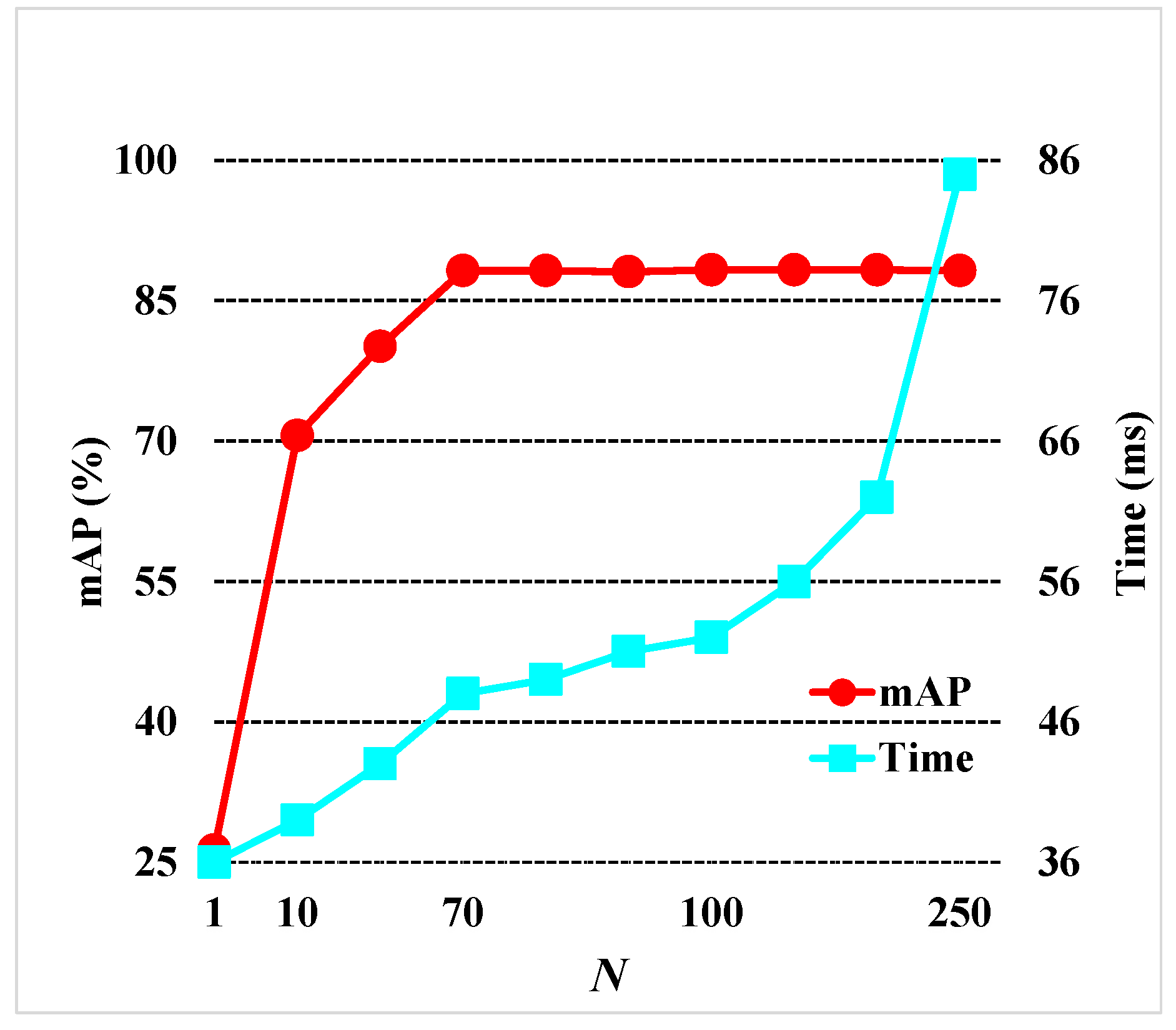
C. Number of sampling pixels for center region prediction network. To reduce the running time, for each image, we randomly sample N ($N=100$) pixels from center regions to generate region proposals. On the one hand, when N is relatively small, the number of generated region proposals is small. Although the running time is short, this is hard for the detection network to produce good detection results. For example, in Figure 11, when $N<70$, the running time is short, but the accuracy is not satisfactory. On the other hand, since the sampled pixels are all from center regions, when N becomes very large, these pixels can be very close to each other. In this situation, the overlaps of generated region proposals can be very high, and most of these region proposals will be eliminated via NMS. As a result, along with the increase of N, the accuracy will no longer increase; however, the running time will become longer. In Figure 11, we can see that when $N>70$, mAP will roughly remain at $88.3\%$, while the running time becomes much longer. For balancing speed and accuracy, we set $N=100$ in the detection network.

D. Scales, aspect ratios, and angles of region proposals.

Table 5. The mAP and the running time for region proposals with different scales.

Setting	Scale	mAP	Running Time
2 scales	64, 256	70.0%	43 ms
3 scales	64, 128, 256	79.9%	47 ms
4 scales	32, 64, 128, 256	88.3%	52 ms
5 scales	32, 88, 144, 200, 256	87.9%	55 ms

lists the detection accuracy and the running time using region proposals with different scales. We can see that for speed/accuracy trade-off, 4-scale region proposals are suitable for the detection network.

Unlike the objects in natural images, for the ships in optical remote sensing images, the ratio of width to height can be very large. To find appropriate aspect ratios of region proposals, we count aspect ratios of rotated boxes in training set (see Figure 12). According to the statistical results, we test different aspect ratios in

Table 6. The mAP and the running time for region proposals with different aspect ratios.

Setting	Aspect Ratio	mAP	Running Time
1 ratio	1:8	87.9%	44 ms
2 ratios	1:4, 1:8	88.3%	52 ms
3 ratios	1:2, 1:5, 1:8	88.4%	58 ms
4 ratios	1:3, 1:5, 1:7, 1:9	88.1%	70 ms

. For balancing accuracy and speed, we set aspect ratios of region proposals as 1:4, 1:8.

3-angle region proposals are used in the detection network. With more angles, the angle difference between the region proposal and the ground-truth box can be small. This is beneficial for producing good detection results, but the running time would become longer (see the fifth column in

Table 7. The mAP and running time for different numbers of angles.

Number of Angle	1 Angle	2 Angles	3 Angles	4 Angles
mAP	78.9%	88.0%	88.3%	88.4%
Running time	42 ms	47 ms	52 ms	57 ms

). On the contrary, when the number of angles is small, the angle difference will be large. Although the running time can be shortened, the detection accuracy would drop (see the second column in Table 7). For speed/accuracy trade-off, 3-angle region proposals are employed in our detection network.

E. Context information of the ship. Context information of ships includes sea, shore, ship, dock, and so on. With the context information, CNN can grasp more useful information. This is beneficial for classification and bounding box regression of the region proposal, producing more accurate detection results. We enlarge the width and the height of the ground-truth box with a factor $\mu$ to use the context information.

Table 8. The mAP for different enlargement factors.

Enlargement Factor $\mathit{\mu }$	1.0	1.2	1.4	1.6
mAP	87.1%	88.1%	88.3%	88.3%

gives mAP using different enlargement factors. We can see that without context information $(\mu =1.0)$, the accuracy is 87.1%, while with context information $(\mu =1.4)$, the accuracy can rise to 88.3%. We set $\mu =1.4$ in this paper.

Finally, we evaluate the detection performance of the proposed method under different ship sizes. We divide the ship objects in remote sensing images into three groups, including small ships ($h^{*}{w}^{*}<{48}^2$), medium ships (${48}^2<h^{*}{w}^{*}<{96}^2$) and relatively large ships ($h^{*}{w}^{*}>{96}^2$). In our dataset, small ships (S), medium ships (M), and relatively large ships (L) account for 36%, 53%, 11%, respectively.

Table 9. The mAP for different ship sizes.

	S	M	L
mAP	81.09%	88.61%	93.70%

lists the detection accuracy under different ship sizes. We can see that as the ship size becomes small, the detection accuracy gradually reduces. The reason is that small ship objects contain less feature information, and are more difficult to be detected. As shown in Table 9, the detection accuracy of the proposed method for small ships can be satisfactory with mAP of about 81%.

6. Conclusions

In this paper, a two-stage ship-detection method is proposed to predict the rotated bounding box from the rotated region proposal. The proposed method constructs the ship orientation classification network to predict angle range of the ship. With the predicted angle range, angle difference between region proposals and ground-truth boxes can be limited to a small value, leading to more accurate region proposals. In addition, center region prediction network predicts the center region of the ship to reduce the number of the region proposal. The two networks share the convolutional features with each other, and generate multi-angle, multi-aspect ratio, and multi-scale region proposals with higher accuracy and smaller number. Experimental results prove that our method can achieve better performance compared with many other state-of-the-art detection methods. Furthermore, we give detailed analysis to prove the reasonability of the proposed detection network. Code is publicly available at https://github.com/JinleiMa/ASD.