Hyperspectral Image Denoising Using Global Weighted Tensor Norm Minimum and Nonlocal Low-Rank Approximation


1
Research & Development Institute of Northwestern Polytechnical University in Shenzhen, Shenzhen 518057, China
2
Ministry of Basic Education, Sichuan Engineering Technical College, Deyang 618000, China
3
Department of Electronics and Informatics, Vrije Universiteit Brussel, 1050 Brussel, Belgium
*
Author to whom correspondence should be addressed.
Remote Sens. 2019, 11(19), 2281; https://0-doi-org.brum.beds.ac.uk/10.3390/rs11192281
Submission received: 6 August 2019
/
Revised: 22 September 2019
/
Accepted: 24 September 2019
/
Published: 29 September 2019
(This article belongs to the Special Issue Advanced Techniques for Spaceborne Hyperspectral Remote Sensing)
Abstract
:A hyperspectral image (HSI) contains abundant spatial and spectral information, but it is always corrupted by various noises, especially Gaussian noise. Global correlation (GC) across spectral domain and nonlocal self-similarity (NSS) across spatial domain are two important characteristics for an HSI. To keep the integrity of the global structure and improve the details of the restored HSI, we propose a global and nonlocal weighted tensor norm minimum denoising method which jointly utilizes GC and NSS. The weighted multilinear rank is utilized to depict the GC information. To preserve structural information with NSS, a patch-group-based low-rank-tensor-approximation (LRTA) model is designed. The LRTA makes use of Tucker decompositions of 4D patches, which are composed of a similar 3D patch group of HSI. The alternating direction method of multipliers (ADMM) is adapted to solve the proposed models. Experimental results show that the proposed algorithm can preserve the structural information and outperforms several state-of-the-art denoising methods.

1. Introduction
A hyperspectral image (HSI) consists of hundreds of contiguous bands at specific wavelengths. They can deliver rich spectral information for real scenes. They have been widely used in many fields, such as urban planning, mapping, agriculture monitoring, forestry, and mineral resources exploration [1,2]. But HSI is unavoidably corrupted by various noises, e.g., Gaussian noise, mixed Poisson–Gaussian noise, dead-lines, and stripes. The noise will influence the subsequent processing, such as classification [3,4,5,6,7], segmentation [8], unmixing [9,10], object detection [11,12], background subtraction [13], and super-resolution [14]. The central limit theorem establishes that the composite effect of many independent noise sources (e.g., thermal noise, shot noise, etc.) should approach a Gaussian distribution. From a practical point of view, current imaging systems designed based on the assumption of additive Gaussian noise perform quite well. As a kind of signal independent noise, the Gaussian assumption has been broadly used in HSI denoising [4,5,6,7,8,9,10,11,12,13,14,15,16,17,18]. From a theoretical point of view, Gaussian noise is the worst-case scenario for additive noise as the Gaussian distribution maximizes the entropy subject to a variance constraint [15]. Therefore, reducing the noise of HSI, especially the Gaussian noise, has been an important preprocessing step in practical applications.
When we add noise to the image to simulate a degraded image, the noise is usually chosen from N(0, Σ), and Σ is the noise covariance matrix which may contain off-diagonal elements. When Σ = σ2Ib, b is the number of bands, and σ2 is the variance of the independent and identically distributed noise. In this case, N(0, Σ) is always written as N(0, σ2) for the sake of simplicity. This represents spectrally uncorrelated noise. In the case of spectrally correlated noise, the noise covariance matrix Σ was generated by:
where is the correlation coefficient between the noise in bands i and (i−1). This is the simple case where the noise in each band is correlated with that of its neighbors. Σ can be adapted to account for more complex interactions. In the literature, additive Gaussian noise is assumed to be spectrally uncorrelated, and the spectrally correlated noise can be transformed to spectrally uncorrelated noise by decorrelation methods. In this paper, we mainly consider reducing the Gaussian noise, which is spectrally uncorrelated.
HSI denoising methods can be classified into different categories from different perspectives. In this work, we classify the HSI denoising methods from the mathematical view. It can be divided into three categories: vectorization, matricization, and tensor (here tensor is especially referred to whose order is more than two). An HSI contains hundreds of spectral channels, and each channel can be regarded as a grayscale image. In the tensor framework, HSI has three modes, one mode is the spectral dimension, the other two are spatial dimensions. Vectorization methods represent the HSI as a vector, such as Spatio-Spectral Total Variation (SSTV) [18], which may result in very high dimensionality and computation complexity. Matricization methods can be divided into two categories. One is band-wise (or band-by-band) processing. Each band of HSI is a gray image, and it can be denoised band-wise by traditional gray-level image denoising methods, such as the nonlocal-based algorithm [19], K-singular value decomposition (K-SVD) [20], and block-matching 3-D filtering (BM3D) [21]. The band-wise methods ignore the correlation in the spectral domain, leading to relatively poor performance. The second category, [10] build the HSI denoising methods under a matrix framework by reshaping an HSI into a matrix, which evidently is more reasonable than band-wise methods. By contrast, though HSI denoising methods based on matrix always outperform the band-wise method, the intrinsic spatial structure of HSI is also inevitably destroyed compared with the methods with the tensor model [22].
Spectral information in an HSI is of great importance in HSI analysis. Therefore, it is essential for HSI denoising techniques to preserve the spectral information. Low rank (LR) prior can reveal the low-dimensional structure in high-dimensional data. It has always been used to regularize the denoising problem [22,23,24]. The tensor-based approach is feasible and effective for HSI processing from a physical point of view. Tensor-based approaches have achieved promising results in HSI denoising [25,26,27,28,29,30,31,32,33,34,35,36] as they can process the spatial and spectral information jointly. Renard et al. [25] proposed a low-rank-tensor-approximation (LRTA) method by employing the Tucker factorization method to obtain the LR approximation of an input HSI. Because LRTA depends on the estimation of the rank of tensor, it may result in unstable results. Liu et al. [27] designed the parallel factor analysis (PARAFAC) method by utilizing the parallel factor analysis [28] to denoise HSI. It regards the two spatial dimensions as two modes of tensor, this will lead to vertical and horizontal artifacts. Xue et al. [29] used the rank-1 tensor decomposition for HSI denoising. However, the number of components of this decomposition cannot be estimated precisely, and the accurate estimation of rank is difficult to guarantee. By jointly considering Tucker and Canonical Polyadic(CP) factorization, a new sparsity measure is presented to characterize tensor data with physical meaning, and it can achieve better recovery from a corrupted multispectral image (MSI) [30].
Considering the nonlocal self-similarity across space in an MSI, a tensor dictionary learning-based (TDL) model [31] is proposed for denoising by enforcing hard constraints on the rank of the core tensor. In real data, this constraint is not guaranteed as the real rank of the core tensor is hard to determine. Yan et al. [34] considered the low-rankness of patches and Hao et al. [35] considered the unfolding matrices low-rankness of HSI. But the former method ignored the correlation of different modes and the latter ignored the global low-rankness of the whole HSI (see Figure 1). Figure 1 illustrates the low-rankness of the unfolding (matricization) of HSI along three modes. The blue curves in Figure 1b,c are the singular values of matrices unfolding along mode-1 and mode-2 (spatial dimension). As both of them show almost the same tendency, it implies they have the same property in the spatial domain along mode-1 and mode-2. The fast decaying trend of the blue curve in Figure 1d indicates the strong correlation along mode-3 (spectral dimension). The yellow squares in Figure 1b–d are examples of similar matrix patches in the unfolding matrices along three modes which imply global similarity of HSI. Similar cube patches in the HSI can be used to enhance denoising performance. Xue et al. [36] have shown good results with nonlocal similarity consideration. However, the singular value of global HSI, or the weighted nuclear norm introduced in [37], should be treated differently to further improve performance. How to fully explore the high correlation and nonlocal similarity is still a challenge for HSI denoising algorithms. By taking into account of the global correlation and nonlocal similarities jointly, we proposed a novel denoising approach.
The main contributions of this paper are three-fold. First, instead of only exploring mode-3 LR prior knowledge of the clean HSI [35], we also consider the LR property of mode-1 and mode-2, which is called global low-rankness. This idea makes full use of the global information in both the spectral and spatial domains.
Second, we use k-nearest neighbor (k-NN) to cluster the nonlocal similar patches (3-order tensor) to construct a 4-order tensor, in which the third dimension is to keep spectral consistent with the HSI itself. These constructed tensors are LR. This is different from the method in [35], which reshapes these similar patches to a new 3-order tensor.
Third, the joint global correlation (GC) and nonlocal low-rankness regularization are integrated into a single scheme, in which the alternative direction minimization method (ADMM) [38,39] is utilized and extended in the proposed model. Extensive experimental testing shows that the proposed method can effectively remove the Gaussian noises and recover details of the original scene. When compared with state-of-the-art methods, the proposed method has done well in both the quantitative evaluation and the visual comparison.
The remainder of this paper is organized as follows: Section 2 reviews the related work and details the proposed method for HSI denoising. Then, the denoising mathematical algorithm and optimization procedure are presented in Section 3. Experimental results and discussions about the experimental results are reported in Section 4 and Section 5, respectively, and conclusions are drawn in Section 5.
2. Materials and Methods
2.1. Motivation
We use boldface Euler script letter (e.g.,), boldface capital letter (e.g., X), boldface lowercase letter (e.g., x), lowercase letter (e.g., ) to denote, respectively, tensor, matrix, vector, and scalar. For an N order tensor , its element at location () is denoted by , where is the real manifold. Its fiber is a vector defined by fixing all indices but one [13]. Its L1 norm and Frobenius norm are defined as and respectively. Matricization (or unfolding) of tensor along mode-n is denoted by , which is obtained by taking all the mode-n fibers to be the columns of the resulting matrix. For a tensor , its n-mode product with a matrix is denoted by . The Tucker decomposition of tensor is defined as a core tensor multiplied by a matrix along each mode [17]: , where is the core tensor of the same size as , and is the orthogonal factor matrix which can be regarded as the principal component in mode i. For more details of tensor formulation, the reader is referred to [13].
The degradation model with additive Gaussian noise of HSI can be represented by , where represent the noisy HSI, clean HSI, and Gaussian noise, respectively, and d, h, b denote the width, height, and number of bands of the HSI, respectively. In this paper, we assume the additive white Gaussian noise is with zero mean and variance σ2.
With the knowledge of LR prior, the denoising problem of matrix X can described as [37]
is the tradeoff parameter. Similarly, the denoising problem of HSI in tensor format can be described as
In the low-rank approximation problem, the nuclear norm is usually introduced as the surrogate functional of LR constraint. The matrix unfolding along mode-3 is LR [22]. Through unfolding along mode-3 with the weighted nuclear norm minimum (WNNM) described in [37], excellent performance in noise removal has been shown in [35]. However, the method in [31] ignores the fact that the unfolding matrix along each mode is coded information which means that both matrices unfolding along mode-1 and mode-2 have the same LR property.
For each matrix, the nuclear norm minimum method treats each singular value equally, and it will lead to a sub-optimum estimation. To overcome this problem, the denoising problem based on the global correlation can be described as
and is the weight nuclear norm of matrix X [37], and w = [w1,w2,…,wn] () is the non-negative weight of σi(X), where , and =0.05 is a constant, is a small number to avoid zero numerator. σi(X) is the i-th largest singular value of X. In this paper, the original HSI is treated as a 3-order tensor, so N=3, and through some experiments, we find that should be equal and they should be smaller than when the denoising result is good. We have conducted various experiments and have empirically chosen
2.2. The Low-Rankness Approximation of Nonlocal Similar Patches Groups
The HSI represents continuous imaging of the same object across the spectral domain. Spectral measurements taken from the same objects or materials in different locations are similar, as they exhibit almost the same spectral reflectance. The patches we call in the following are referred to as 3-D full-band patches (FBPs). As these patches contain the nonlocal similarity information in the spatial domain and the global correlation information across all spectral bands, they are usually used as prior knowledge in denoising methods [22,31]. However, the matricization method usually concatenates the patches to a matrix, this procession always results in spectral distortion. Based on GC prior, noise in the HSI will be removed globally, but local spatial and spectral distortion will appear, and there will be much residual noise. The distortion and residual noise can be removed efficiently based on nonlocal low-rank regularization [40], which uses nonlocal self-similarity (NSS) to characterize HSI [41]. The similarity is evaluated by the Frobenius norm of the Euclidean distance of given two patches. Smaller norms represent a higher similarity [42].
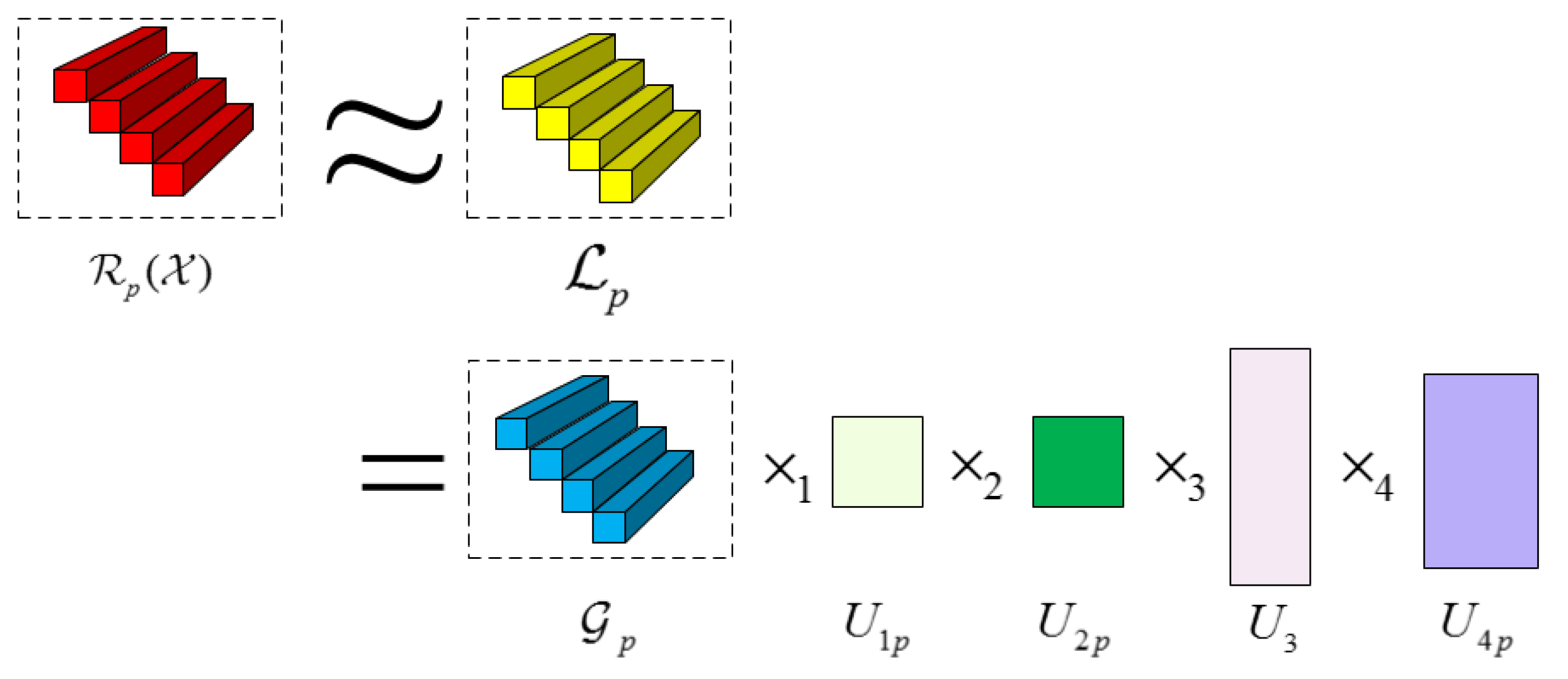
Motivated by [30], we separate noisy-free HSI into many overlapped 3D patches of the size , where t×t is the spatial dimension, and b is the number of bands of HSI. These patches are collected in a patch set , where Γ represents the index set and is the i-th 3D patch in this set. For each exemplar patch , we search for its similar patches by k-nearest neighbor (k-NN) [43,44] method in the spatial domain. Here, two patches are considered similar if the Euclidean distance between two patch vectors is smaller than a given threshold. For each 3D patch of , we search for similar 3D patches from a big window around this 3D patch. Then can be grouped into J clusters and these similar 3D patches in each cluster are reshaped into a 4-order tensor of size , where p is the index of the p-th cluster, as shown in Figure 2, and N0 is the number of patches. The selection of J is illustrated in Section 4.4. It is more reasonable than reshaping each cluster into a 3-order tensor, as described in [30]. Because the patches in each cluster have very similar structures, can be approximated by a LR tensor , i.e., . The corresponding optimization problem is
As an HSI has strong correlation across the spectrum, is LR. The patches in each cluster have a very similar structure which implies that is also LR. So can be represented by Tucker decomposition: , where is core tensor, and are factor matrices orthogonal in columns, e.g., , 3=I. Note that the factor matrices in the spectral mode for all p are set as a shared matrix , insuring that is low-rank in the spectral mode on the whole. Similar to the global denoising problem, the ideal HSI’s patches can be estimated by solving the following optimization problem:
where is tensor norm described in (1).
By replacing in (6) with the corresponding Tucker decomposition, we obtain the following problem:
where is core tensor.
2.3. Proposed Method
Considering both global and nonlocal low-rankness, we propose the following regularized optimization problem:
The unconstrained version of (8) is
3. Optimization Procedure and Algorithm Results
The scheme of the proposed HSI denoising method is summarized in Figure 3. To solve the proposed denoising model, we apply the variable splitting technique [39], and introduce new auxiliary variables and (p = 1,2,...,K). Replacing variable in the second term and in the third term, problem (8) can be reformulated as
By introducing two proper parameters, α and β, (10) can be changed to the unconstrained version:
The proposed algorithm for denoising can now be summarized in Algorithm 1. Please refer to the Appendix A for the detail of the optimization process with this algorithm.
| Algorithm 1. Proposed method for HSI denoising |
| Input: Noisy HSI Output: Denoised HSI Initialization: Set parameters α, β, λ, μ, η, R1 = ceil(h ×0.6) and R2 = ceil(d×0.6); is initialized by (R1, R2, R3)-Tucker approximation of , here ceil(a) indicates the smallest integer larger than a. Other variables are initialized by 0. 1: while not converged do 2: updating via 3: updating via 4: updating via 5: updating via 6: updating via 7: updating via 8: updating via 9: updating via , where 10: updating α=1.05α, β=1.05β 11: end while |
4. Experimental Results and Discussion
Experiments on both simulated and real HSI data were executed to qualitatively and quantitatively assess the denoising performance of the proposed approach. We implemented five state-of-art HSI denoising methods for comparison, namely HyRes [22], LRTA [25], PARAFAC [27], tensor dictionary learning (TDL) [30], Intrinsic Tensor Sparsity (ITSReg) [31], and, tensor singular value decomposition (t-SVD) [32]. Here, the first four compared algorithms were based on tensor, although the last one was based on matrix, but it can deal with 3-D HSI data such as tensor, so we choose it to compare with the proposed method. Their implementation codes can be directly obtained from the authors’ websites. In our experiments, the parameter settings of the compared methods were the default setting provided in the reference papers.
4.1. Experiment on Simulated Noisy Data
The first simulated experiments were conducted with the Washington D.C. dataset (WDC for short) (https://engineering.purdue.edu/~biehl/MultiSpec/hyperspectral.html). This image comprised 1280 lines and 307 columns, with a spatial resolution of 3m and 210 bands. We extracted a 341×307 sub-image, and the bands which were seriously degraded were removed. The data were normalized to the range of [0, 1], and the variance of added noise varied from 0.1 to 0.3.
Five quantitative image quality assessment indices (IQAs) were employed for performance evaluation, including peak signal-to-noise ratio (PSNR) [45], structure similarity (SSIM) [45], erreur relative globale adimensionnelle de synthese (ERGAS) [46],feature similarity (FSIM) [47], and spectral angle mapper (SAM) [48]. PSNR and SSIM were utilized to evaluate the similarity between the target image and the reference image based on mean squared error (MSE) and structural consistency, respectively. The unit of PSNR was dB. The FSIM was utilized to evaluate the perceptual consistency with the reference image. Larger values of these three measures represent better results. ERGAS measures fidelity of the restored image based on the weighted sum of MSE in each band, and SAM calculates the average angle between spectrum vectors of the target HSI and the reference one across all spatial positions, so it fully reflects the fidelity of the spectral reflectance of the target HSI. However, different from the former three measures, smaller values of these two measures represent better denoising results of the HSI. In this paper, the denoising IQAs (MPSNR, MSSIM, MFSIM, MERGAS, or MSAM) for each HSI were calculated as the average of all the bands.
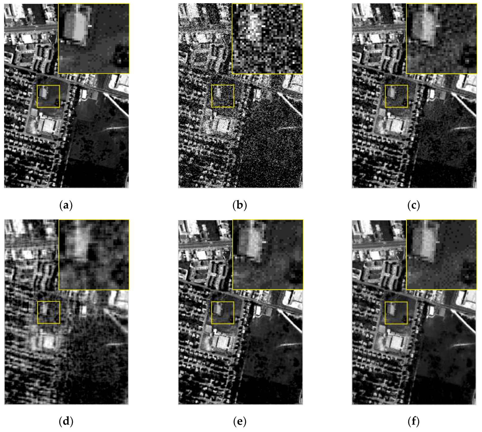
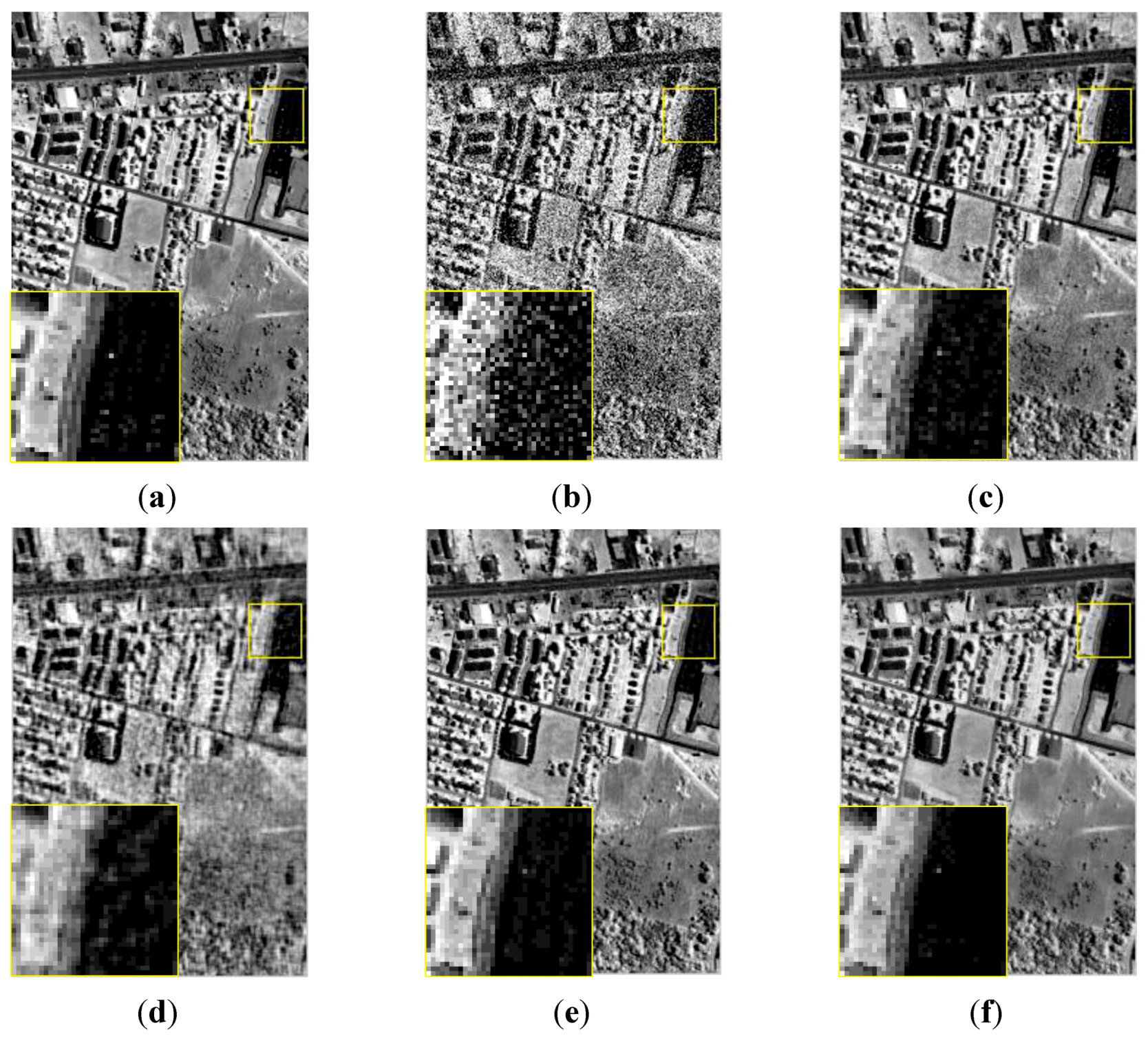
The performances of all methods on WDC dataset at different noise intensity levels are listed in Table 1. It can be found that the indices of the proposed method with ERGAS and SAM were lower than the compared methods, while the other three indices of the proposed method were higher than these methods. The visual superiority of our method with the results of compared methods is also obvious. To further depict the visual denoising performance of our method, the denoising results under variance 0.3 are shown in Figure 4 with a false-color image. The red, green, and blue channels are the composition of bands 60, 27, and 17 as described in https://engineering.purdue.edu/~biehl/MultiSpec/hyperspectral.html. It is observed from the enlarged part of the denoising results that there were obvious visual artifacts in the results of the PARAFAC and LRTA. The visual artifacts of the PARAFAC came from the fact that the two spatial dimensions should not be considered as two modes of tensor. With such decomposition, the outer products will lead to vertical and horizontal artifacts(see Figure 4d, Figure 5d, and Figure 6d). The details were over-smoothed with t-SVD and ITSReg, as shown in the zoomed square. The TDL considers only the nonlocal similarity but ignores the global correlation, so the reconstructed HSI by TDL was not so completed compared with the proposed method. Even though the false-color image of HyRes looks similar to the proposed method, blurred parts are still observed from the enlarged part. To verify the effectiveness of the algorithm in different datasets and at different noise intensity levels, the Urban dataset with size 301×201×162 was used. Figure 5 and Figure 6 show the denoising results with noise variance 0.2 of band 42 and 74, respectively. A similar conclusion can be drawn in the experiment on this dataset (see Table 2 and Figure 5 and Figure 6). Our algorithm not only suppresses noise but also preserves image details and texture.
As shown by the enlarged part of the denoising results, PARAFAC fails to maintain the structural integrity and generated obvious artifacts because it lacks accurate estimation for the rank of HSI. The result of LRTA still has much residual noise. As an extension of matrix singular value decomposition, the t-SVD still treats each singular value equally in the diagonal. It usually results in over-smooth in some regions and leaves residual noise in others. Although TDL considers nonlocal similarity in the spectral domain, it has higher spectral distortion and cannot preserve the details. While ITSReg has considered the intrinsic structure, it ignores the nonlocal similarity. The HyRes shows almost the same performance as the proposed method. By comparing with the LRTA, PARAFAC, TDL, t-SVD, and ITSReg, the proposed method produces better results on Gaussian noise removal. As we consider the global correlation and nonlocal similarity, it achieves the better visual outcome and spectral fidelity. Figure 7 shows the PSNR, SSIM, and FSIM values of each band of the Urban dataset with noise variance at 0.2. The PSNR, SSIM, and FSIM values of the proposed method are higher than those of the compared methods, indicating better noise removal.
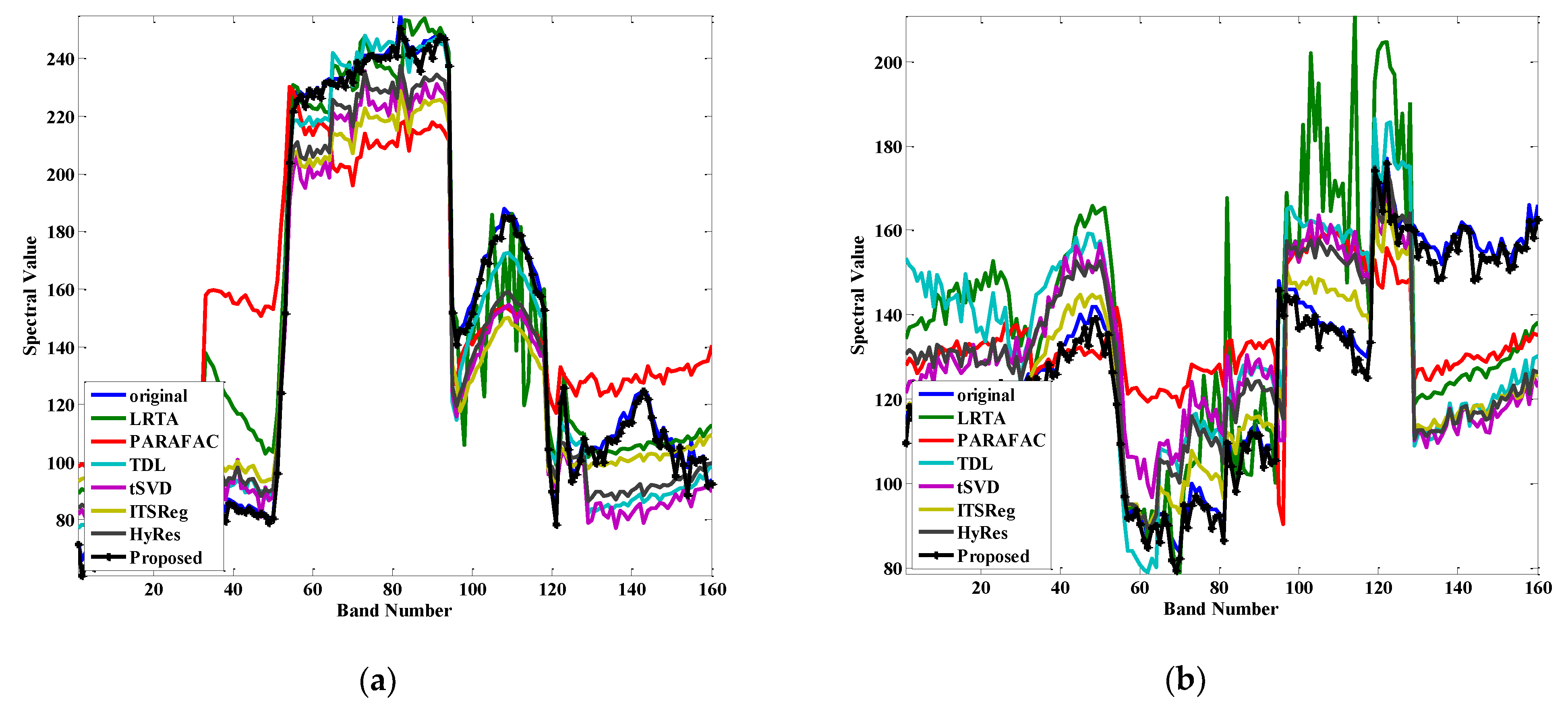
To further investigate the performance of preserving useful spectral information while removing noise, we plotted the spectral values curve at spatial locations (100,100) and (150,150) in Figure 8a,b, respectively. The results are contrast-stretched to 0–255 for better visualization. The closer to the original spectrum means the spectral information preservation is better. Though the HyRes showed almost the same performance with the proposed method, it showed severe distortion in various bands. The same results have been observed with the other five compared methods. This result is in consistency with the IQAs and visual inspection mentioned above.
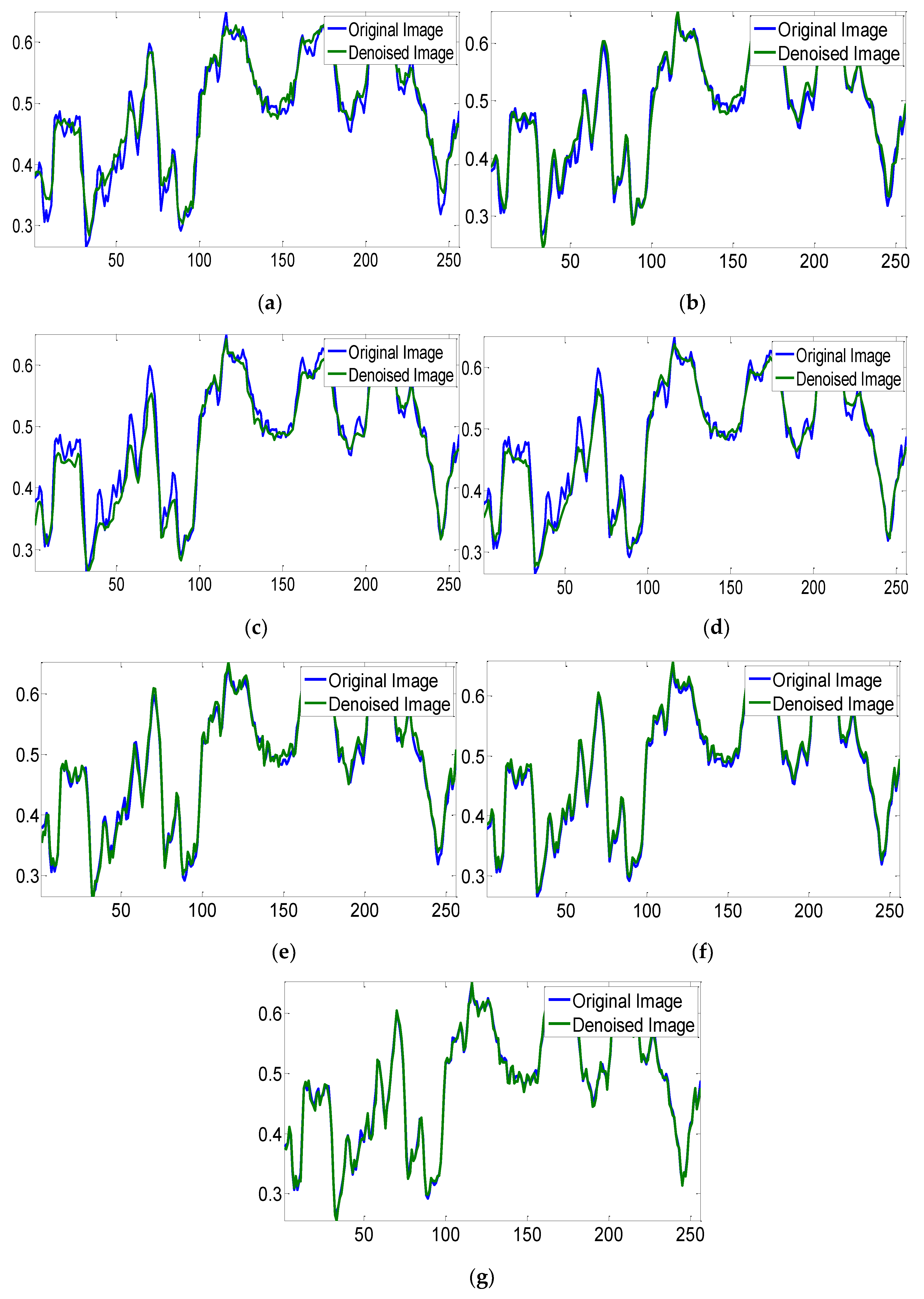
To give some qualitative comparison, the qualitative index of the mean cross-track profile was adopted. We show the horizontal mean profiles of 35th band in Indian Pine set before and after denoising in Figure 9. The horizontal axis in Figure 9 represents the row number, and the vertical axis represents the mean digital number values of each row. As shown in Figure 9a, the curve has sharp fluctuation because of the noise. The fluctuation is more or less suppressed by all the methods. The proposed method provides evidently smoother curves while preserving the spatial information.
4.2. Real HSI Denoising
In this section, we present the results of the Indian Pine dataset (https://engineering.purdue.edu/~biehl/MultiSpec/hyperspectral.html). Its size is 145 × 145 × 220, and spatial resolution is 20 m. The implementation strategies and parameter settings for all competing methods were the same as the above-simulated experiments. Since the noise level was unknown, we used the no-reference HSI quality assessment (NHQA for short) [49] method, which is based on quality-sensitive features. The results are listed in Table 3, from which we see that the value of the proposed method was lower than others, which indicates better performance.
By analyzing Table 1, Table 2 and Table 3, we can conclude that the proposed method works better than compared methods, no matter what the noise level and testing data (synthetic data or real data) are. It demonstrates the potentials of the global and nonlocal low-rank constraints in our algorithm. The proposed algorithm provides competitive results to the state-of-the-art algorithms.
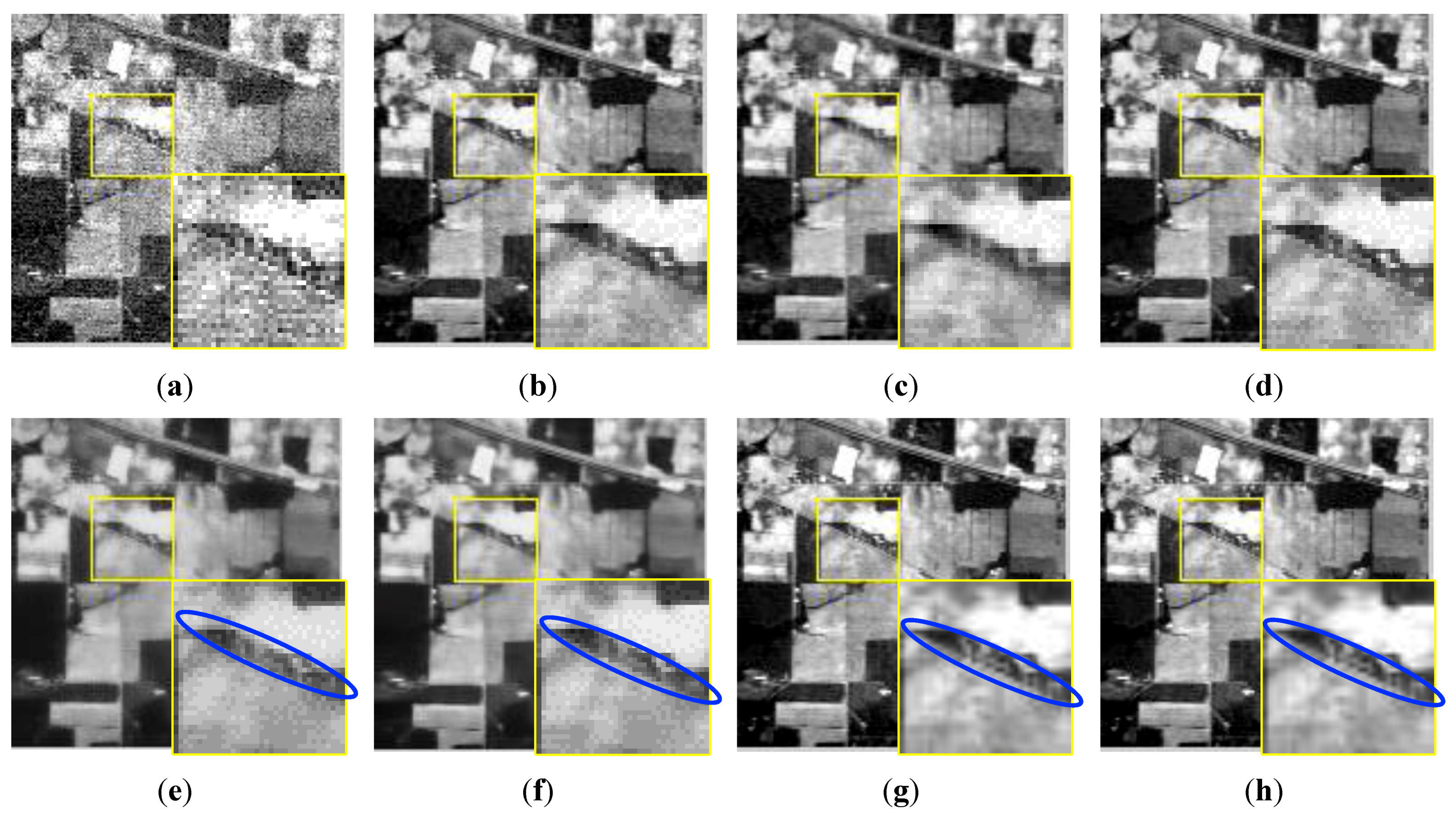
Figure 10 shows the 107th band of the restored images obtained by all competing methods. Figure 10a shows that the original HSI bands were corrupted by heavy noise. Although the restored results from Figure 10b to Figure 10f look satisfactory, in Figure 10b–d, there still exists residual noise, and Figure 10e,f show over-smooth with missing details. Comparatively, albeit less prior knowledge was considered, our method can better restore textures and edge details, and manage to remove structural noises, as shown in Figure 10h. Some stripes and random noises were removed. This further substantiates the robustness of the proposed method.
4.3. Compare of Computational Costs
In this section, we compared the computational costs of different models for these datasets: the WDC (size 341 × 307 × 160), URBAN (size 145 × 145 × 220), and Indian Pine (size 145 × 145 × 220). The running time (in seconds) for the denoising task by LRTA, PARAFAC, TDL, t-SVD, ITSReg, and the proposed method are listed in Table 4. All the experiments were implemented on Windows 7, the Core i5-7300HQ, [email protected] GHz, and the 8 G memory platform by MATLAB R2014a.
The LRTA method is the fastest. But its denoising performance is lower compared to the other methods. The proposed method needs to search for similar 3D patches and the optimization procedure with Tucker decomposition. Both make it relatively slow. For the optimization procedure, though each sub-problem has the closed-form solution in the ADMM framework, the operation time is still long. For future work, we intend to investigate how to reduce the processing time. Although the HyRes obtains similar performance both qualitatively and quantitatively, it can be observed from Figure 8 and Figure 9 that the denoised HSI suffers from spectral distortion.
4.4. Parameter Selection and Analysis of Convergence
In Algorithm 1, there are eight parameters, i.e., α, β, λ, μ, η, R1, R2, and R3. Since the auxiliary variable should be close to the estimated . The regularization parameter will gradually increase, where the error between the two variables will decrease with increasing iterations. In all experiments, we initialize as 10 and updated it by = 1.05 * . Similarly, we initialized β=10 and updated it by new β = 1.05*β. The R1 and R2 for factor matrices U1 and U2 control the complexity of spatial redundancy. They were empirically set as R1 = ceil(h ×0.6) and R2=ceil(d×0.6) in all conducted experiments as this setting works fairly well. The R3, which controls the complexity of temporal redundancy, should be carefully tuned with each dataset. We set R3 as 1 for the real-world datasets.
The parameter λ controls the error of LR approximation. In our experiments with simulated data, we initialized λ = 40/σ and λ = 10/σ for WDC dataset and Indian Pine dataset, respectively. The σ here is the variance of Gaussian noise. For the real data experiments, we set λ = 1.5 in the first iteration. Then, we gradually increased the value of λ with error decreasing.
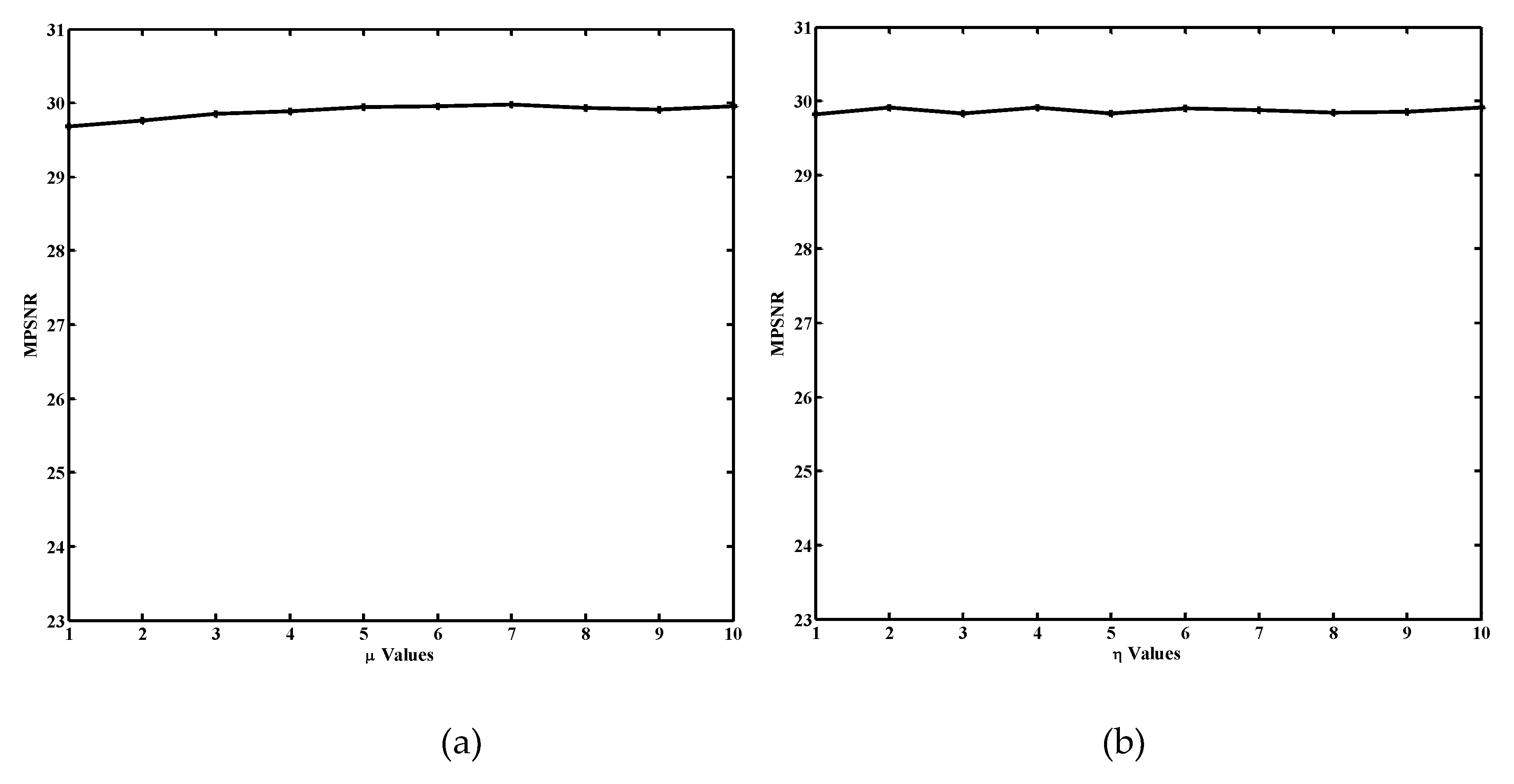
The parameters of μ and η balanced the regularizations from the spectral domain and spatial domain, respectively. To determine the optimal values of these two parameters, we conducted simulated experiments. Figure 11 shows the example using mean PSNR (MPSNR) as the selection criterion, then a greedy strategy was applied to select the parameter values one by one. Although the parameters obtained by this method are not global optimum, it has achieved favorable denoising performance.
The function curve of MPSNR values with the regularization parameters μ and η are plotted in Figure 11a,b. MPSNR is insensitive to different values of μ and η. Therefore, we can conclude that the proposed method is robust with any μ and η. For convenience, we set μ and η to 1 in all the experiments with both simulated and real datasets.
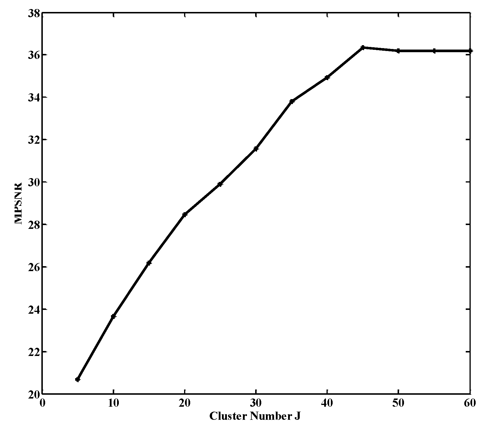
Additionally, we conducted experiments to understand the best number of clusters J. The results of MPSNR versus the J are displayed in Figure 12. When J = 45, it achieved the best MPSNR. We also observe that MPSNR declined slightly when J was increased from 45 to 60. This is mainly because the similarity within a cluster cannot be guaranteed when J is too large. In other words, the parameter J is optimal when the denoising performance has reached a plateau.
4.5. Analysis of Convergence
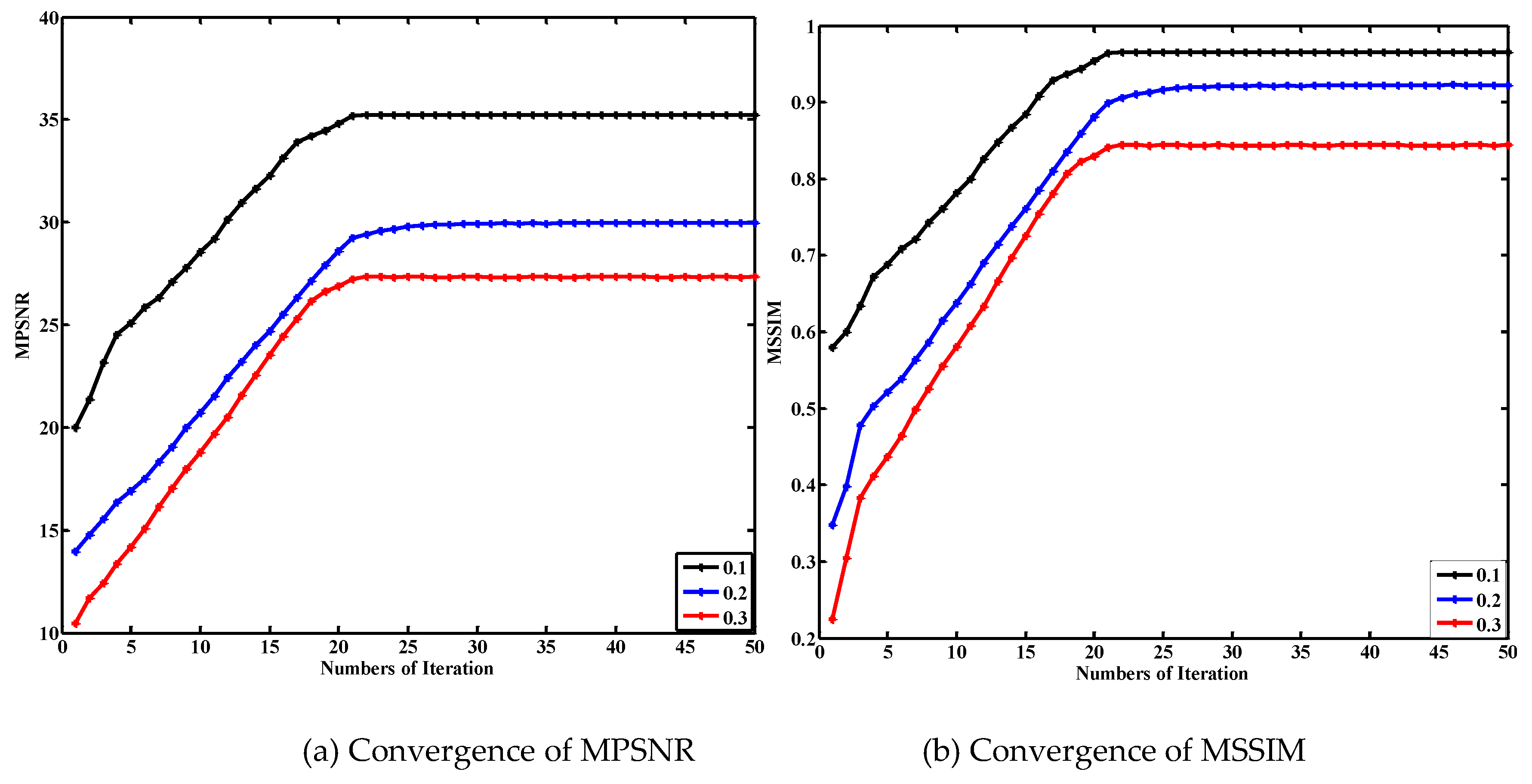
To illustrate the convergence of the proposed algorithm, we provide the convergence curves with MPSNR and MSSIM of the Urban dataset. The curves under different noise levels are shown in Figure 13a,b. It can be seen that the values of MPSNR and MSSIM do not change after about 20 iterations. In addition, we also provide the convergence curves of the synthetic WDC dataset and Indian Pine dataset in Figure 14a,b. The objective function values were used as the assessment index of algorithm convergence. The steepest decline happened in the first 20 iterations.
4.6. A comparison of State-of-the-Art Clustering Methods
In Table 5, the proposed tensor-based learning, traditional deep learning method, and the clustering approach in [7] are compared. Both of the clustering approach in [7] and our proposed method can be regarded as tensor-based learning. However, there are still some differences. The main difference is that the clustering approach in [7] is CP (rank-1) decomposition (CPD), while our method is built on Tucker decomposition (TD). For each constructed 4-D tensor, which possesses the two local spatial modes, one spectral mode, and one nonlocal spatial mode, each mode has a specific physical meaning. Compared to CPD without reasonable interpretation to descript information prior to each mode, TD has a stronger ability to characterize the low-rank property of HSI. For other differences, please refer to Table 5.
5. Conclusions
In this paper, we proposed an HSI denoising method by jointly utilizing nonlocal and global low-rankness of HSI. Global low-rankness was exploited via three modes unfolding matrices. This approach exploited the structural information of the original HSI. To take advantage of nonlocal similarity, an LR constraint was added as regularization. This approach was also utilized to exploit the original structural information of image patches and structured sparsity of similar patches. We also split the variables and designed an efficient ADMM algorithm to solve the model. From the experiments with both simulated and real datasets, we conclude that the proposed method based on the intrinsic features of GC and NSS is more efficient. The values of ERGAS and SAM were lower while the FSIM, SSIM, and PSNR were higher (Table 1 and Table 2). Figure 8 and Figure 9 illustrate the efficiency of the proposed method where spectral features and spatial features were more consistent with the references. The experimental results demonstrate that our method can achieve competitive performance compared with other state-of-the-art methods. However, the parameters have to be selected experimentally, and the time cost is considered high. This is a disadvantage. In the future, we will concentrate on accelerating the speed of the algorithm to improve its practical significance.
Author Contributions
X.K. contributed to the research experiments, data analysis, and writing of the paper. Y.Z. helped to design the experiments and research analysis. J.X. collected and preprocessed the original data. J.C.-W.C. helped the with analysis and writing of the paper. All co-authors helped to revise the manuscript.
Funding
This work is supported by National Natural Science Foundation of China (NSFC) (61771391, 61371152), Science Technology Innovation Commission of Shenzhen Municipality (JCYJ20170815162956949, JCYJ20180306171146740) and the Innovation Foundation for Doctor Dissertation of Northwestern Polytechnical University (CX201917).
Acknowledgments
Our gratitude goes to the anonymous reviewers and editors for their careful work and thoughtful suggestions that have improved this paper substantially.
Conflicts of Interest
The authors declare no conflict of interest.
Appendix A. Optimization Process of Algorithm 1
The ADMM strategy is introduced to optimize the objective function (11):
(I) Optimizing :
This is a weighted tensor nuclear minimum problem, and its closed-form solution is given in [41], that is , where .
(II) Optimizing :
Here we omit the ∑ for simplicity. Similar to sub-problem (I), the closed-form solution is , where .
(III) Optimizing :
The optimization problem in (A2) can be approximated by alternatively updating the following formulas:
where is unit tensor, , SVD(A,r) indicates top r singular vectors of matrix A, and eigs(A,r) indicates top r eigenvectors of matrix A. Let us denote the rank constraint of U1, U2, and U3 by R1, R2, and R3. The proposed algorithm for denoising can now be summarized in Algorithm 1.
(IV) Optimizing :
The vectorization of (A9) is
The solution of (A10) is
where
where = Vec() is vectorization of tensor Ten(x) is tensorization of vector x, i.e., the inverse operation of Vec.
References
- Rasti, B.; Scheunders, P.; Ghamisi, P.; Licciardi, G.; Chanussot, J. Noise Reduction in Hyperspectral Imagery: Overview and Application. Remote Sens. 2018, 10, 482. [Google Scholar] [CrossRef]
- Han, J.; Zhang, D.; Cheng, G.; Guo, L.; Ren, J. Object detection in optical remote sensing images based on weakly supervised learning and high-level feature learning. IEEE Trans. Geosci. Remote Sens. 2015, 53, 3325–3337. [Google Scholar] [CrossRef]
- Zhang, L.; Zhang, L.; Tao, D.; Huang, X. On Combining Multiple Features for Hyperspectral Remote Sensing Image Classification. IEEE Trans. Geosci. Remote Sens. 2012, 50, 879–893. [Google Scholar] [CrossRef]
- Li, J.; Zhang, H.; Huang, Y.; Zhang, L. Hyperspectral image classification by nonlocal joint collaborative representation with a locally adaptive dictionary. IEEE Trans. Geosci. Remote Sens. 2014, 52, 3707–3719. [Google Scholar] [CrossRef]
- Fang, L.; Li, S.; Kang, X.; Benediktsson, J.A. Spectral–spatial hyperspectral image classification via multiscale adaptive sparse representation. IEEE Trans. Geosci. Remote Sens. 2014, 52, 7738–7749. [Google Scholar] [CrossRef]
- Zhao, Y.; Zhang, G.; Jie, F.; Gao, S.; Chen, C.; Pan, Q. Unsupervised Classification of Spectropolarimetric Data by Region-Based Evidence Fusion. IEEE Geosci. Remote Sens. Lett. 2011, 8, 755–759. [Google Scholar] [CrossRef]
- Makantasis, K.; Doulamis, A.D.; Doulamis, N.D.; Nikitakis, A. Tensor-based classification models for hyperspectral data analysis. IEEE Trans. Geosci. Remote Sens. 2018, 56, 6884–6898. [Google Scholar] [CrossRef]
- Li, J.; Bioucas-Dias, J.M.; Plaza, A. Semisupervised hyperspectral image segmentation using multinomial logistic regression with active learning. IEEE Trans. Geosci. Remote Sens. 2010, 48, 4085–4098. [Google Scholar] [CrossRef]
- Yi, C.; Zhao, Y.Q.; Yang, J.; Chan, J.C.W.; Kong, S.G. Joint Hyperspectral Super-Resolution and Unmixing with Interactive Feedback. IEEE Trans. Geosci. Remote Sens. 2017, 55, 3823–3834. [Google Scholar] [CrossRef]
- Yang, J.; Zhao, Y.-Q.; Chan, J.C.-W.; Kong, S.G. Coupled Sparse Denoising and Unmixing with Low Rank Constraint for Hyper-spectral Image. IEEE Trans. Geosci. Remote Sens. 2016, 54, 1818–1833. [Google Scholar] [CrossRef]
- Gao, S.B.; Cheng, Y.M.; Zhao, Y.Q.; Xiao, L.-P. Data-driven quadratic correlation filter using sparse coding for infrared targets detection. J. Infrared Millim. Waves 2014, 33, 498–506. [Google Scholar] [CrossRef]
- Xue, J.; Zhao, Y.; Liao, W.; Chan, J.C.-W. Hyper-Laplacian Regularized Nonlocal Low-rank Matrix Recovery for Hyperspectral Image Compressive Sensing Reconstruction. Inf. Sci. 2019, 501, 406–420. [Google Scholar] [CrossRef]
- Xue, J.; Zhao, Y.; Liao, W.; Chan, J.C.-W. Total Variation and Rank-1 Constraint RPCA for Background Subtraction. IEEE Access 2018, 6, 49955–49966. [Google Scholar] [CrossRef]
- Yi, C.; Zhao, Y.Q.; Chan, J.C.W. Spectral super-resolution for multispectral image based on spectral improvement strategy and spatial preservation strategy. IEEE Trans. Geosci. Remote Sens. 2019, 1–15. [Google Scholar] [CrossRef]
- Shomorony, I.; Avestimehr, A.S. Worst-Case Additive Noise in Wireless Networks. IEEE Trans. Inf. Theory 2013, 59, 3833–3847. [Google Scholar] [CrossRef] [Green Version]
- Kolda, T.G.; Bader, B.W. Tensor decompositions and applications. J. SIAM Rev. 2005, 66, 294–310. [Google Scholar] [CrossRef]
- Lathauwer, L.D.; Moor, B.D.; Vandewalle, J. A multilinear singular value decomposition. SIAM J. Matrix Anal. Appl. 2000, 21, 1253–1278. [Google Scholar] [CrossRef]
- Aggarwal, H.K.; Majumdar, A. Hyperspectral Image Denoising Using Spatio-Spectral Total Variation. IEEE Geosci. Remote Sens. Lett. 2016, 13, 442–446. [Google Scholar] [CrossRef]
- Buades, A.; Coll, B.; Morel, J.-M. A non-local algorithm for image denoising. In Proceedings of the IEEE Computer Society Conference on Computer Vision and Pattern Recognition, San Diego, CA, USA, 20–25 June 2005; pp. 60–65. [Google Scholar] [CrossRef]
- Elad, M.; Aharon, M. Image denoising via sparse and redundant representations over learned dictionaries. IEEE Trans. Image Process. 2006, 15, 3736–3745. [Google Scholar] [CrossRef] [PubMed]
- Dabov, K.; Foi, A.; Katkovnik, V.; Egiazarian, K. Image denoising by sparse 3-D transform-domain collaborative filtering. IEEE Trans. Image Process. 2007, 16, 2080–2095. [Google Scholar] [CrossRef]
- Rasti, B.; Ulfarsson, M.O.; Ghamisi, P. Automatic Hyperspectral Image Restoration Using Sparse and Low-Rank Modeling. IEEE Geosci. Remote Sens. Lett. 2017, 14, 2335–2339. [Google Scholar] [CrossRef] [Green Version]
- Zhao, Y.Q.; Yang, J. Hyperspectral Image Denoising via Sparse Representation and Low-Rank Constraint. IEEE Trans. Geosci. Remote Sens. 2015, 53, 296–308. [Google Scholar] [CrossRef]
- Xue, J.; Zhao, Y.; Liao, W.; Chan, J.C.-W. Nonlocal Tensor Sparse Representation and Low-Rank Regularization for Hyperspectral Image Compressive Sensing Reconstruction. Remote Sens. 2019, 11, 193. [Google Scholar] [CrossRef]
- Renard, N.; Bourennane, S.; Blanc-Talon, J. Denoising and dimensionality reduction using multilinear tools for hyperspectral images. IEEE Trans. Geosci. Remote Sens. 2008, 5, 138–142. [Google Scholar] [CrossRef]
- Xue, J.; Zhao, Y.; Liao, W.; Kong, S.G. Joint Spatial and Spectral Low-Rank Regularization for Hyperspectral Image Denoising. IEEE Trans. Geosci. Remote Sens. 2018, 56, 1940–1958. [Google Scholar] [CrossRef]
- Liu, X.; Bourennane, S.; Fossati, C. Denoising of hyperspectral images using the parafac model and statistical performance analysis. IEEE Trans. Geosci. Remote Sens. 2012, 50, 3717–3724. [Google Scholar] [CrossRef]
- Sena, M.M.; Trevisan, M.G.; Poppi, R.J. Parallel factor analysis. In Practical Three-Way Calibration; Elsevier: Amsterdam, The Netherlands, 2005; pp. 109–125. [Google Scholar] [CrossRef]
- Xue, J.; Zhao, Y.; Liao, W.; Chan, J.C.-W. Nonconvex tensor rank minimization and its applications to tensor recovery. Inf. Sci. 2019, 503, 109–128. [Google Scholar] [CrossRef]
- Xie, Q.; Zhao, Q.; Meng, D.; Xu, Z.; Gu, S.; Zuo, W.; Zhang, L. Multispectral Images Denoising by Intrinsic Tensor Sparsity Regularization. In Proceedings of the IEEE Conference on Computer Vision and Pattern Recognition, Las Vegas, NV, USA, 27–30 June 2016; pp. 1692–1700. [Google Scholar] [CrossRef]
- Peng, Y.; Meng, D.; Xu, Z.; Gao, C.; Yang, Y.; Zhang, B. Decomposable Nonlocal Tensor Dictionary Learning for Multispectral Image Denoising. In Proceedings of the IEEE Conference on Computer Vision and Pattern Recognition, Columbus, OH, USA, 23–28 June 2014; pp. 2949–2956. [Google Scholar] [CrossRef]
- Drineas, P.; Mahoney, M.W. A randomized algorithm for a tensor-based generalization of the singular value decomposition. Linear Algebra Appl. 2007, 420, 553–571. [Google Scholar] [CrossRef] [Green Version]
- Buades, A.; Coll, B.; Morel, J.-M. A review of image denoising algorithms, with a new one. Multiscale Model. Simul. 2005, 4, 490–530. [Google Scholar] [CrossRef]
- Yan, L.; Fang, H.; Zhong, S.; Zhang, Z.; Chang, Y. Weighted Low-rank Tensor Recovery for Hyperspectral Image Restoration. arXiv 2017, arXiv:1709.00192. [Google Scholar]
- Hao, R.; Su, Z. A patch-based low-rank tensor approximation model for multiframe image denoising. J. Comput. Appl. Math. 2018, 329, 125–133. [Google Scholar] [CrossRef]
- Xue, J.; Zhao, Y.; Liao, W.; Chan, J.C.-W. Nonlocal Low-Rank Regularized Tensor Decomposition for Hyperspectral Image Denoising. IEEE Trans. Geosci. Remote Sens. 2019, 57, 5174–5189. [Google Scholar] [CrossRef]
- Gu, S.; Zhang, L.; Zuo, W.; Feng, X. Weighted Nuclear Norm Minimization with Application to Image Denoising. In Proceedings of the IEEE Conference on Computer Vision and Pattern Recognition, Columbus, OH, USA, 23–28 June 2014; pp. 2862–2869. [Google Scholar] [CrossRef]
- Boyd, S.; Parikh, N.; Chu, E.; Peleato, B.; Eckstein, J. Distributed optimization and statistical learning via the alternating direction method of multipliers. Found. Trends Mach. Learn. 2011, 3, 1–122. [Google Scholar] [CrossRef]
- Fu, Y.; Wang, R.; Jin, Y.; Zhang, H. Fast image fusion based on alternating direction algorithms. In Proceedings of the 12th International Conference on Signal Processing, Alsace, France, 20–22 July, 2015; pp. 713–717. [Google Scholar] [CrossRef]
- Dong, W.; Li, G.; Shi, G.; Li, X.; Ma, Y. Low-Rank Tensor Approximation with Laplacian Scale Mixture Modeling for Multiframe Image Denoising. In Proceedings of the IEEE International Conference on Computer Vision (ICCV), Santiago, Chile, 7–13 December 2015; pp. 442–449. [Google Scholar] [CrossRef]
- Zhang, C.; Hu, W.; Jin, T.; Mei, Z. Nonlocal image denoising via adaptive tensor nuclear norm minimization. Neural Comput. Appl. 2016, 29, 3–19. [Google Scholar] [CrossRef]
- Peng, X.; Lu, C.; Yi, Z.; Tang, H. Connections Between Nuclear Norm and Frobenius Norm Based Representations. IEEE Trans. Neural Netw. Learn. Syst. 2015, 29, 218–224. [Google Scholar] [CrossRef] [PubMed]
- Peng, X.; Feng, J.; Xiao, S.; Yau, W.Y.; Zhou, J.T.; Yang, S. Structured AutoEncoders for Subspace Clustering. IEEE Trans. Image Process. 2018, 27, 5076–5086. [Google Scholar] [CrossRef] [PubMed]
- Peng, X.; Yu, Z.; Yi, Z.; Tang, H. Constructing the L2-Graph for Robust Subspace Learning and Subspace Clustering. IEEE Trans. Cybern. 2012, 47, 1053–1066. [Google Scholar] [CrossRef] [PubMed]
- Wang, Z.; Bovik, A.; Sheikh, H.; Simoncelli, E. Image quality assessment: From error visibility to structural similarity. IEEE Trans. Image Process. 2004, 13, 600–612. [Google Scholar] [CrossRef]
- Wald, L. Data Fusion: Definitions and Architectures. Fusion of Images of Different Spatial Resolutions; Presses de l’Ecole, Ecole des Mines de Paris: Paris, France, 2002. [Google Scholar]
- Zhang, L.; Zhang, L.; Mou, X.; Zhang, D. Fsim: A feature similarity index for image quality assessment. IEEE Trans. Image Process. 2011, 20, 2378–2386. [Google Scholar] [CrossRef] [PubMed]
- Du, P.; Chen, Y.; Fang, T.; Tang, H. Error analysis and improvements of spectral angle mapper (SAM) model. In MIPPR 2005: SAR and Multispectral Image Processing; International Society for Optics and Photonics: Bellingham, WA, USA, 2005; pp. 1–6. [Google Scholar] [CrossRef]
- Yang, J.; Zhao, Y.; Yi, C.; Chan, J.C.W. No-Reference Hyperspectral Image Quality Assessment via Quality-Sensitive Features Learning. Remote Sens. 2017, 9, 305. [Google Scholar] [CrossRef]
Figure 1.
Illustration of global spatial-and-spectral correlation in hyperspectral images (HSI). (a) Original HSI and (b) the matrix unfolding by mode-1 and its singular value curve; (c) the matrix unfolding by mode-2 and its singular values curve, and (d) the matrix unfolding by mode-3 and its singular values curve. The x-label is the length of the unfolding matrix.

Figure 2.
The 4-order tensor grouped in each cluster can be reconstructed by low-rank Tucker decomposition.
Figure 2.
The 4-order tensor grouped in each cluster can be reconstructed by low-rank Tucker decomposition.

Figure 3.
Scheme of the proposed HSI denoising method using global and nonlocal low-rank (LR) regularizations.
Figure 3.
Scheme of the proposed HSI denoising method using global and nonlocal low-rank (LR) regularizations.

Figure 4.
Simulated noise removal results on Washington D.C. (WDC) data at band 10 (noise variance is 0.3). (a) Original image. (b) Noisy image. Denoising results by (c) low-rank-tensor-approximation (LRTA), (d) parallel factor analysis (PARAFAC), (e) tensor dictionary learning (TDL), (f) tensor singular value decomposition (t-SVD), (g) Intrinsic Tensor Sparsity (ITSReg), (h) HyRes, (i) Proposed.

Figure 5.
Visual quality comparison of the denoising results of band 42 with noise variance 0.2. (a) Original image. (b) Noisy image. Denoising results by (c) LRTA, (d) PARAFAC, (e) TDL, (f) t-SVD, (g) ITSReg, (h) HyRes, (i) Proposed
Figure 5.
Visual quality comparison of the denoising results of band 42 with noise variance 0.2. (a) Original image. (b) Noisy image. Denoising results by (c) LRTA, (d) PARAFAC, (e) TDL, (f) t-SVD, (g) ITSReg, (h) HyRes, (i) Proposed


Figure 6.
Visual quality comparison of the denoising results of band 74 with noise variance 0.2. (a) Original image. (b) Noisy image. Denoising results by (c) LRTA, (d) PARAFAC, (e) TDL, (f) t-SVD, (g) ITSReg, (h) HyRes, (i) Proposed.
Figure 6.
Visual quality comparison of the denoising results of band 74 with noise variance 0.2. (a) Original image. (b) Noisy image. Denoising results by (c) LRTA, (d) PARAFAC, (e) TDL, (f) t-SVD, (g) ITSReg, (h) HyRes, (i) Proposed.


Figure 7.
Comparison of IQAs of the denoising results with variance 0.20 Gaussian noise: including (a) peak signal-to-noise ratio (PSNR), (b) structure similarity (SSIM), and (c) feature similarity (FSIM), (d) erreur relative globale adimensionnelle de synthese (ERGAS), (e) spectral angle mapper (SAM).

Figure 8.
Comparison of spectral reflectance value at location (a) (100,100), (b) (150,150) under variance 0.20 Gaussian noise.
Figure 8.
Comparison of spectral reflectance value at location (a) (100,100), (b) (150,150) under variance 0.20 Gaussian noise.

Figure 9.
Horizontal mean profiles of 35th band in WDC data, the horizontal axis represents the row number, and the vertical axis represents the mean digital number values of each row. (a) LRTA, (b) PARAFAC, (c) TDL, (d) tSVD, (e) ITSReg, (f) HyRes, (g) Proposed.
Figure 9.
Horizontal mean profiles of 35th band in WDC data, the horizontal axis represents the row number, and the vertical axis represents the mean digital number values of each row. (a) LRTA, (b) PARAFAC, (c) TDL, (d) tSVD, (e) ITSReg, (f) HyRes, (g) Proposed.

Figure 10.
Visual quality comparison of the denoising results of all methods on band 107 in Indian Pine HSI data. (a) Original image, (b) LRTA, (c) PARAFAC, (d) TDL, (e) t-SVD, (f) ITSReg, (g) HyRes, (h) Proposed.
Figure 10.
Visual quality comparison of the denoising results of all methods on band 107 in Indian Pine HSI data. (a) Original image, (b) LRTA, (c) PARAFAC, (d) TDL, (e) t-SVD, (f) ITSReg, (g) HyRes, (h) Proposed.

Figure 11.
Sensitivity analysis of parameter: (a) Relationship between mean PSNR (MPSNR) and μ. (b) Relationship between MPSNR and η.
Figure 11.
Sensitivity analysis of parameter: (a) Relationship between mean PSNR (MPSNR) and μ. (b) Relationship between MPSNR and η.

Figure 12.
Relationship between MPSNR and the cluster number J.

Figure 13.
Curves of (a) MPSNR, (b) MSSIM of URBAN dataset under noise levels 0.1, 0.2, and 0.3.

Figure 14.
Convergence curves for (a) WDC dataset under noise level 0.2 and (b) Indian Pine dataset.
Figure 14.
Convergence curves for (a) WDC dataset under noise level 0.2 and (b) Indian Pine dataset.


Table 1.
Average performance of six competing methods with respect to five IQAs on the WDC dataset.
| Variance | Index | Noisy Image | LRTA | PARAFAC | TDL | t-SVD | ITSReg | HyRes | Proposed |
|---|---|---|---|---|---|---|---|---|---|
| 0.1 | MERGAS | 235.618 | 80.934 | 205.254 | 58.892 | 66.516 | 66.400 | 53.142 | 51.285 |
| MFSIM | 0.837 | 0.951 | 0.842 | 0.977 | 0.973 | 0.973 | 0.989 | 0.989 | |
| MSSIM | 0.713 | 0.937 | 0.741 | 0.970 | 0.968 | 0.966 | 0.984 | 0.986 | |
| MPSNR | 19.993 | 29.580 | 21.209 | 32.313 | 31.156 | 31.096 | 33.015 | 33.212 | |
| MSAM | 0.3420 | 0.1258 | 0.1082 | 0.0776 | 0.0610 | 0.0602 | 0.0488 | 0.0481 | |
| 0.2 | MERGAS | 471.236 | 128.882 | 208.844 | 99.246 | 106.972 | 123.583 | 90.942 | 90.867 |
| MFSIM | 0.711 | 0.908 | 0.839 | 0.951 | 0.941 | 0.925 | 0.961 | 0.967 | |
| MSSIM | 0.452 | 0.870 | 0.732 | 0.931 | 0.922 | 0.895 | 0.944 | 0.951 | |
| MPSNR | 13.973 | 25.354 | 21.057 | 27.619 | 26.910 | 25.630 | 27.983 | 28.375 | |
| MSAM | 0.5428 | 0.1473 | 0.1112 | 0.0875 | 0.0717 | 0.0724 | 0.0681 | 0.0621 | |
| 0.3 | MERGAS | 706.855 | 165.924 | 214.940 | 132.553 | 142.304 | 164.568 | 125.017 | 124.803 |
| MFSIM | 0.620 | 0.874 | 0.833 | 0.925 | 0.905 | 0.875 | 0.937 | 0.944 | |
| MSSIM | 0.293 | 0.807 | 0.718 | 0.885 | 0.868 | 0.820 | 0.896 | 0.904 | |
| MPSNR | 10.451 | 23.088 | 20.805 | 25.032 | 24.400 | 23.127 | 25.16 | 25.814 | |
| MSAM | 0.6901 | 0.1402 | 0.1162 | 0.0898 | 0.0704 | 0.0727 | 0.0614 | 0.0698 |
Table 2.
Average performance of six competing methods with respect to five IQAs on the URBAN dataset.
Table 2.
Average performance of six competing methods with respect to five IQAs on the URBAN dataset.
| Variance | Index | Noisy Image | LRTA | PARAFAC | TDL | t-SVD | ITSREG | HyRes | Proposed |
|---|---|---|---|---|---|---|---|---|---|
| 0.1 | MERGAS | 304.984 | 89.666 | 253.521 | 69.326 | 79.281 | 76.134 | 63.81 | 64.371 |
| MFSIM | 0.831 | 0.960 | 0.829 | 0.974 | 0.971 | 0.972 | 0.988 | 0.989 | |
| MSSIM | 0.580 | 0.905 | 0.655 | 0.948 | 0.943 | 0.946 | 0.951 | 0.965 | |
| MPSNR | 19.992 | 30.798 | 21.604 | 33.087 | 31.916 | 32.159 | 35.074 | 35.108 | |
| MSAM | 0.514 | 0.124 | 0.167 | 0.086 | 0.093 | 0.083 | 0.064 | 0.068 | |
| 0.2 | MERGAS | 609.968 | 151.650 | 258.479 | 117.230 | 127.088 | 140.455 | 111.057 | 110.847 |
| MFSIM | 0.698 | 0.911 | 0.825 | 0.944 | 0.937 | 0.924 | 0.957 | 0.960 | |
| MSSIM | 0.348 | 0.802 | 0.643 | 0.887 | 0.882 | 0.869 | 0.904 | 0.915 | |
| MPSNR | 13.972 | 26.119 | 21.435 | 28.443 | 27.676 | 26.777 | 29.684 | 29.975 | |
| MSAM | 0.775 | 0.175 | 0.177 | 0.1104 | 0.108 | 0.103 | 0.098 | 0.091 | |
| 0.3 | MERGAS | 914.952 | 201.083 | 266.740 | 155.195 | 168.758 | 191.443 | 146.910 | 146.281 |
| MFSIM | 0.604 | 0.871 | 0.819 | 0.914 | 0.900 | 0.875 | 0.907 | 0.928 | |
| MSSIM | 0.224 | 0.719 | 0.625 | 0.833 | 0.821 | 0.791 | 0.851 | 0.862 | |
| MPSNR | 10.450 | 23.630 | 21.160 | 25.930 | 25.168 | 24.060 | 27.021 | 27.380 | |
| MSAM | 0.934 | 0.184 | 0.191 | 0.117 | 0.112 | 0.112 | 0.115 | 0.103 |
Table 3.
Comparison of no-reference HSI quality assessment (NHQA) in [49] on Indian Pine dataset.
Table 3.
Comparison of no-reference HSI quality assessment (NHQA) in [49] on Indian Pine dataset.
| LRTA | PARAFAC | TDL | t-SVD | ITSReg | HyRes | Proposed | |
|---|---|---|---|---|---|---|---|
| NHQA | 27.3619 | 27.4287 | 27.1911 | 27.1038 | 27.1360 | 26.9105 | 26.8241 |
Table 4.
Comparisons of computational time for the denoising methods (in second).
| Size | LRTA | PARAFAC | t-SVD | TDL | ITSReg | HyRes | Proposed | |
|---|---|---|---|---|---|---|---|---|
| WDC | 341 × 307 × 160 | 48 | 269 | 4.2306 × 10⁴ | 113 | 10.6579 × 10⁴ | 159 | 9.16 × 10⁴ |
| URBAN | 301 × 201 × 162 | 27 | 132 | 0.2531 × 10⁴ | 45 | 1.0631 × 10⁴ | 136 | 4.921 × 10⁴ |
| Indian Pine | 145 × 145 × 220 | 104 | 2237 | 0.1968 × 10⁴ | 175 | 0.5053 × 10⁴ | 182 | 2.184×10⁴ |
Table 5.
Comparisons of differences between tensor-based learning and traditional deep learning.
| Proposed Approach | Approach of [7] | Traditional Deep Learning | |
|---|---|---|---|
| layer of prior | single | single | multi |
| time cost | low | low | high |
| Learning method | on-line | on-line | off-line |
| decomposition | tucker | rank-1 canonical | — |
| labeled training samples | — | large number | large number |
| tunable parameters | small | small | huge |
| spatial and spectral structure | integrated | integrated | destroyed |
| computational complexity | low | low | high |
| classification accuracy | low | high | high |
© 2019 by the authors. Licensee MDPI, Basel, Switzerland. This article is an open access article distributed under the terms and conditions of the Creative Commons Attribution (CC BY) license (http://creativecommons.org/licenses/by/4.0/).
Share and Cite
MDPI and ACS Style
Kong, X.; Zhao, Y.; Xue, J.; Chan, J.C.-W. Hyperspectral Image Denoising Using Global Weighted Tensor Norm Minimum and Nonlocal Low-Rank Approximation. Remote Sens. 2019, 11, 2281. https://0-doi-org.brum.beds.ac.uk/10.3390/rs11192281
AMA Style
Kong X, Zhao Y, Xue J, Chan JC-W. Hyperspectral Image Denoising Using Global Weighted Tensor Norm Minimum and Nonlocal Low-Rank Approximation. Remote Sensing. 2019; 11(19):2281. https://0-doi-org.brum.beds.ac.uk/10.3390/rs11192281
Chicago/Turabian StyleKong, Xiangyang, Yongqiang Zhao, Jize Xue, and Jonathan Cheung-Wai Chan. 2019. "Hyperspectral Image Denoising Using Global Weighted Tensor Norm Minimum and Nonlocal Low-Rank Approximation" Remote Sensing 11, no. 19: 2281. https://0-doi-org.brum.beds.ac.uk/10.3390/rs11192281
Note that from the first issue of 2016, this journal uses article numbers instead of page numbers. See further details here.