Ice-Gouging Topography of the Exposed Aral Sea Bed
by
 , , ,
, , ,
Stepan Maznev
1,* ,
,
Stanislav Ogorodov
1 ,
,
Alisa Baranskaya
1,
Aleksey Vergun
1,2,
Vasiliy Arkhipov
1,2 and
Peter Bukharitsin
3 1
Laboratory of Geoecology of the North, Faculty of Geography, Lomonosov Moscow State University, Leninskie Gory, Moscow 119991, Russia
2
Zubov State Oceanographic Institute, Kropotkinsky lane 6, Moscow 119034, Russia
3
Water Problems Institute, Russian Academy of Sciences, Tatischeva street 16, Astrakhan 414056, Russia
*
Author to whom correspondence should be addressed.
Remote Sens. 2019, 11(2), 113; https://0-doi-org.brum.beds.ac.uk/10.3390/rs11020113
Submission received: 15 November 2018
/
Revised: 24 December 2018
/
Accepted: 4 January 2019
/
Published: 9 January 2019
(This article belongs to the Special Issue Mass Movement and Soil Erosion Monitoring Using Remote Sensing)
Abstract
:Ice gouging, or scouring, i.e., ice impact on the seabed, is a well-studied phenomenon in high-latitude seas. In the mid-latitudes, it remains one of the major geomorphic processes in freezing seas and large lakes. Research efforts concerning its patterns, drivers and intensity are scarce, and include aerial and geophysical studies of ice scours in the Northern Caspian Sea. This study aims to explain the origin of the recently discovered linear landforms on the exposed former Aral Sea bottom using remotely sensed data. We suggest that they are relict ice gouges, analogous to the modern ice scours of the Northern Caspian, Kara and other seas and lakes, previously studied by side scan sonar (SSS) surveys. Their average dimensions, from 3 to 90 m in width and from hundreds to thousands of meters in length, and spatial distribution were derived from satellite imagery interpretation and structure from motion-processing of UAV (unmanned aerial vehicle) images. Ice scouring features are virtually omnipresent at certain seabed sections, evidencing high ice gouging intensity in mid-latitude climates. Their greatest density is observed in the central part of the former East Aral Sea. The majority of contemporary ice gouges appeared during the rapid Aral Sea level fall between 1980 and the mid-1990s. Since then, the lake has almost completely drained, providing a unique opportunity for direct studies of exposed ice gouges using both in situ and remote-sensing techniques. These data could add to our current understanding of the scales and drivers of ice impact on the bottom of shallow seas and lakes.
1. Introduction
Sea ice as a zonal factor is associated with high latitudes and plays an important role in the evolution of the coasts and seabed in polar regions [1,2,3,4]. It can execute direct mechanical, thermal, physical and chemical impact on the coasts and bottom [1,5,6]. However, ice can also affect the coasts and bottom of freezing seas and large lakes in mid-latitudes [7,8,9], in particular, of the Caspian [10,11,12,13] and Aral Seas. The most dangerous and impressive process driven by ice is mechanical plowing of bottom ground called ice gouging. It is associated with ice cover movement, ice hummocking (ridging) and formation of grounded hummocks (stamukhas) under the influence of hydrometeorological factors and coastal topography [3,14,15]. Ice gouging significantly changes bottom topography and can affect engineering facilities, e.g., oil and gas pipelines [13,16,17,18].
Studies of ice effect on the seabed in the middle latitudes started back in the 1950s in the Northern Caspian Sea [10]. Soviet researchers described traces of sea ice impact using aerial imagery. Such traces were best seen in shallow zones at depths of 1–3 m in wave-protected inlets [19]. With the onset of modern geophysical methods, further investigations at the Northern Caspian in March 2008 showed ice scours with lengths exceeding several kilometers. The width of single scours reached 5 m; the width of their combs was up to 200 m; the depth of the scours reached 1 m [12]. In North America, J. Grass [7] first described deep ice keels scouring the bottom of Lake Erie down to depths of 25 m, penetrating loose sediments down to approximately 2 m. More studies of the Great Lakes followed [20,21,22]. In [23], ice conditions during 41 years are compared with extensive statistics on ice scours. Discoveries of ice scours on land were described near lake Ontario [24], where they were possibly made by icebergs, in the sediments of Scarborough Bluffs, Toronto [25,26], and even at Racetrack Playa, California, where they were created by ice-rafting rocks [27].
The present study aims to characterize ice-gouging processes and landforms at the Aral Sea bed, their origin and evolution. The Aral Sea (Figure 1) is a unique site for studies of ice gouging, as most of its bottom is now exposed after a rapid water level decline. Modern remote sensing methods provide an opportunity to detect ice scours on the surface of the former sea bottom, as well as at shallow depths under water (usually not exceeding 3 m). The possibility of direct in situ observations allows detailed studies of the ice gouges’ morphology and distribution.
Scours at the exposed bottom of the former Aral Sea were first discovered on aerial photographs in 1990 by B. Smerdov from the Hydrometeorological Institute of Kazakhstan [28]. He made a field description of the landforms and a trial pit and showed that traces on the Aral seabed are up to 8 km long, look like a “comb” and reach 0.4–0.5 m in depth. However, Smerdov rejected the version that such landforms appeared by ice gouging and interpreted them as traces of divine origin or traces of aliens’ activity. Detailed academic studies of ice gouging at the bottom of the Aral Sea started very recently [29]; until now, no consistent descriptions and investigations of these landforms were made.
Here, we use high-resolution satellite imagery along with field surveys to characterize ice gouging landforms and reconstruct mechanisms of ice impact on the Aral Sea bottom. We also estimate its main climatic drivers and compare the landforms on the exposed bottom of the Aral Sea to relatively well studied ice gouges of the Caspian Sea and Arctic seas.
2. Site Description
The Aral Sea is located in an inland cold desert. The summer is dry and hot; the winter is cold with unstable weather [30,31]. In November, air temperature in the northern part of the sea drops below zero; the average temperature of January is −11…−13 °C. In the southern part of the sea, the average temperature of January is −6…−8 °C. The period with negative temperatures lasts for 120–150 days [32]. In winter, when the Siberian Atmospheric Pressure High affects the vast area of the Aral Sea, invasions of cold air masses from the north and northwest provide rapid temperature drops. In warm seasons, when the Siberian High recedes, the South Asian Low affects the region, and winds from eastern directions persist. In March, air temperature quickly rises to +5…+10 °C.
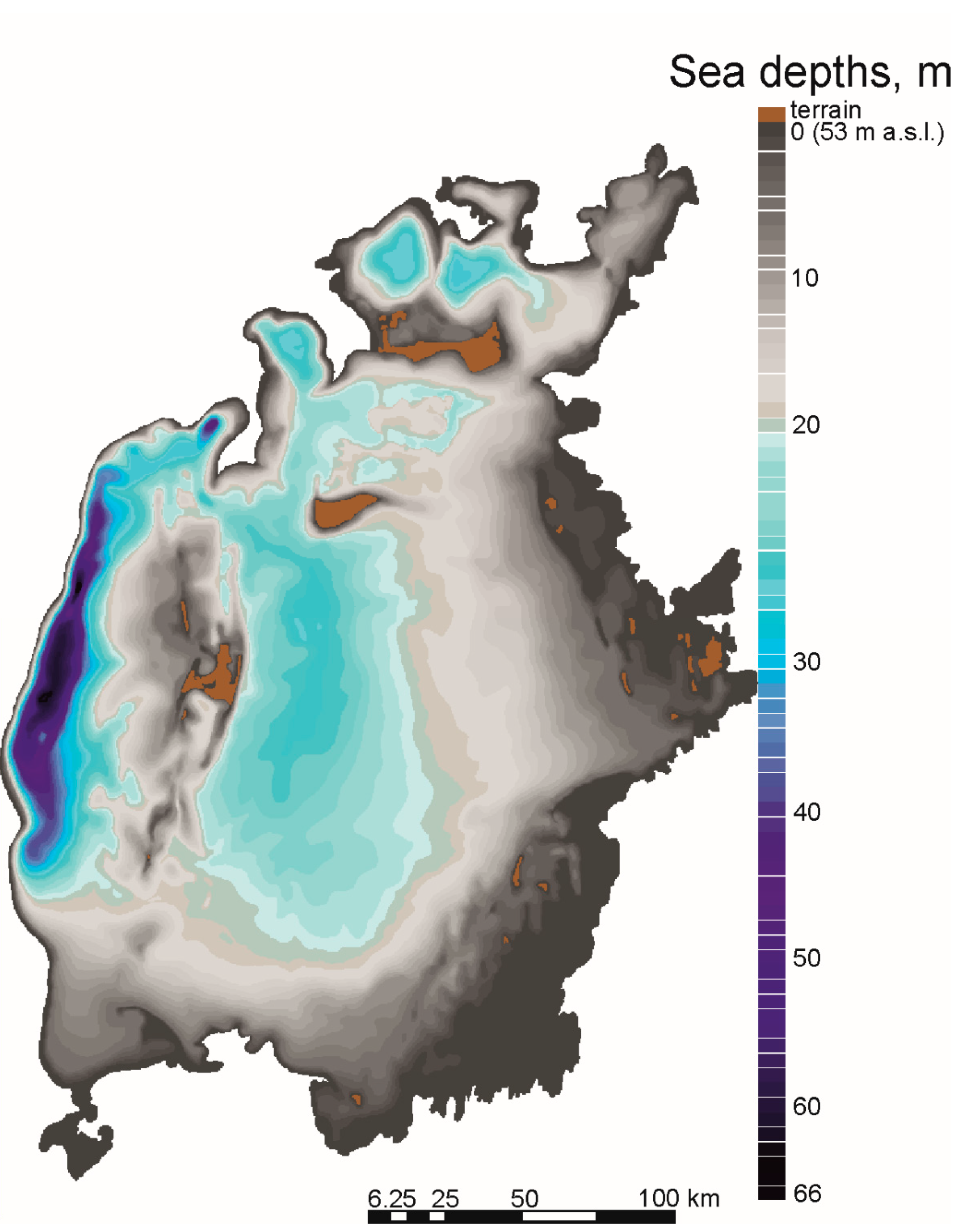
Depths of the Aral Sea at its greatest extent before the 1960s reached 60 m (Figure 2). The bottom topography of its eastern part was extremely flat with a mean inclination of 1–2‰ and depths of 10–20 m. The central parts of the North and East Aral Sea are flat wide depressions with former water depths from 20 to 30 m. The greatest depths of up to 65 m were observed in the West Aral Sea, stretching in a narrow patch from the north to the south along its western coast. The steep western underwater slope of the depression is a continuation of the Ustyurt Plateau chink down in the Aral Sea.
Before 1960, water level in the Aral Sea was at the elevation of 53 m a.s.l. (above mean sea level) (Figure 2). In 1961, it started to decline as a result of the flow redistribution of Syr Darya and Amu Darya rivers discharging into it. After extensive water use for irrigation of cotton and rice fields, these rivers could not further sustain the water balance of the Aral Sea, and evaporation exceeded discharge. Consequently, the Aral Sea experienced a fast level drop. In 55 years, the water level lowered by more than 30 m in some locations (Figure 3). Because of the level decrease, in 1986, the lake split into the North and South Aral Seas, which started to retreat separately. In 2007, the South Aral Sea was divided into the West and East Aral Seas (Figure 3 and Figure 4). Today, the water level of the North Aral Sea is at 42 m, the level of the West Aral Sea is at 23.5 m. The level of the East Aral Sea was at 28.5 m, before it dried out completely by 2014 [33,34,35].
The salinity of the Aral Sea increased significantly as a result of water level decrease. In 1961, the average salinity of the Aral Sea water was about 10‰; by 1990, it had increased to 32‰. In 2008, the salinity of the Western Aral Sea exceeded 100‰, and the Eastern Aral Sea had the salinity of 210‰ [37].
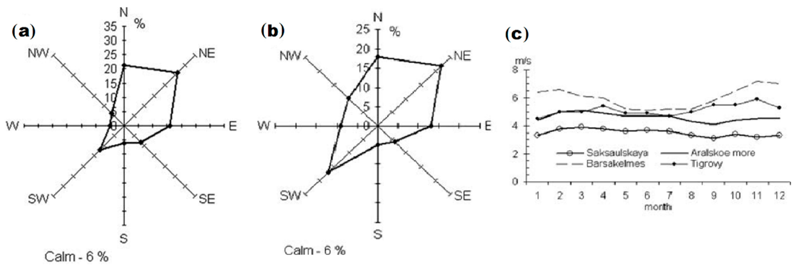
Ice conditions of the lake during its high level position in the past were favorable for ice gouging. Before the 1960s, the Aral Sea usually began freezing up in November, reaching its maximum extent in mid-February. Fast ice covered the coastal zone of the sea, reaching 20–30 km in width in the north; open areas were occupied by drifting ice consisting of brash ice and ice fields. Ice thickness ranged from up to 65–70 cm in the north to 35–45 cm in the south. Fast ice was broken up repeatedly by strong winds during the freeze-up, and drifted offshore. Because of strong northeasterly winds (up to 35% occurrence in the cold period) (Figure 5), rafted ice and hummocky formations were appearing. Northerly and easterly winds pushed the ice to the southern part of the sea, causing its high concentration in the south [38]. Ice was starting to melt in the second half of February and completely disappeared by the end of April [32].
After the water level drop, ice conditions became more severe. Along with the decrease in water area, the Aral Sea froze up faster and several days earlier; ice melting began later and lasted longer [39]. Results of satellite imagery monitoring in 1982–2009 confirm significant changes in the thermal and ice conditions compared to the quasi-undisturbed period before 1961, resulting from shallowing and heat content lowering, along with the decrease in temperatures of the water layer immediately below the ice [40,41]. Therefore, the climate of the Aral Sea region, similarly to the Northern Caspian region [30], provided favorable conditions for ice scouring of the bottom by hummocks both before and during the water level fall. Strong winds and presence of drifting ice for up to 6 months gives evidence of permanent mass movement of large ice fields, while the presence of relatively vast shallows both before and after the water level fall implies that the keels must have penetrated into the bottom ground causing extensive formation of ice scours (Figure 6).
3. Materials and Methods
3.1. Remote Sensing
For documentation of ice gouging topography on vast territories of the former Aral Sea bottom, high-resolution imagery with significant spatial coverage was required. We analyzed the exposed bottom of both the North and South Aral Seas within the limits of the shoreline of 1960, as well as shallow waters down to 3 m depth, estimating the bottom coverage by scours. A key area in the northeastern part of the East Aral Sea (Figure 4) was subject to more detailed studies with analysis of the morphologic and morphometric parameters of the scours, their directions and distribution.
The whole area of investigations within the shoreline of 1960 (about 50,000 km2) is comparable to areas of average European countries, e.g., Estonia. Using commercial products such as WorldView or QuickBird for such large areas would immensely increase the cost of investigations. Because our aims did not require the processing of multitemporal data, we used public open source imagery taken not earlier than 2010, when, as we assume, the intensity of ice gouging at the Aral Sea significantly reduced. We used WorldView, QuickBird, Sentinel, IKONOS, and GeoEye images taken from Bing [43], Yandex [44], Google [45] websites and ESRI [42], the combination of which covered the whole study area without clouds, deep water areas, etc. The imagery was georeferenced and interpreted in ArcGIS 10.2 (ESRI Inc., Redlands, CA, USA).
Optical imagery allows ice scours and other forms of ice impact on the bottom to be distinguished due to the difference in spectral reflectance. However, the scours can be both brighter and darker than the background surface, and may have a complicated shape. Therefore, we considered manual selection of the scours to be most reliable. An important step was separating the forms of ice impact on the exposed bottom from other linear objects, above all, erosional landforms, identifiable by their sinuosity or flow marks (typical stream textures), and roads, characterized by fixed width. As a result of the imagery interpretation, we obtained linear shapefiles showing the scours.
In total, we processed 138 scours within the key area in the northeast of the Aral Sea (Figure 4). For each of them, we determined:
- its length as the sum of its straight segments;
- its typical or average width (in case of significant difference between segments, the width of single scours and “combs” was determined);
- its general direction, defined as the direction between the end points or, in case of a complex shape, the direction of the longest segments;
- the order of the scours’ appearance in case of their imposition;
- the number of single scours in a comb (in case of multiple gouges).
The obtained data were further statistically processed in Ms Excel. For all parameters, maximum, minimum and average values, standard deviations, and coefficients of variation were calculated.
To estimate the bottom coverage by the ice scours and their distribution, areas with similar patterns and a visually similar coverage (n = 46) were selected. Within these areas, small experimental key sites (e.g., 1 × 1 km) were assigned, where the surface affected by ice gouging was deciphered using polygon ArcGIS shapefiles, and the percentage of land coverage by ice gouges was calculated. These values were extrapolated to larger previously selected areas (n = 22 after merging), and grouped into intervals reflecting the degree of ice impact, in order to create a scheme of the whole former Aral Sea bed. Such assessment is quantitative and precise for the experimental key sites only; for larger areas it is based on visual similarity and expert opinion, being a qualitative estimation, allowing to reveal general patterns only.
3.2. Photogrammetric Field Investigations and Data Processing
During fieldwork conducted in October 2018 in the northeastern part of the East Aral Sea (Polygons 1–5, Figure 4), fragments of ice gouges on the former bottom were shot by an unmanned aerial vehicle (UAV) with subsequent ortho-photo mosaic and digital elevation model (DEM) creation. A DJI Phantom 4 Professional Drone was used [46]; the photographs were taken from the nadir (vertical) viewing direction. Flying missions were planned using the Android application PIX4DCapture [47]. The size of the investigated polygons varied depending on local conditions, generally being several hundred meters (e.g., 500 × 500 m). The UAV survey took place at a height of 50 or 100 m, depending on the required resolution with traverses along or across the polygon. The shooting was done with an overlap of 60–80%, allowing to obtain a high-resolution DEM. The shooting frequency was 30 frames per minute. Parameters of the UAV surveys and their accuracy are shown in Table 1.
For referencing of the surveys, a network of ground control points (GCPs) was used. The GCPs were 15 × 20 cm black and white paper markers placed in the corners and center of each polygon. Georeferencing of the GCPs was performed by Javad Maxor GNSS (global navigation satellite system) receivers with an accuracy of about 1 cm in plan and 2 cm in height. One of the GNSS receivers was installed above the main GCP with a survey peg; the rest of the GCPs were referenced by another receiver. Polygons were referenced to each other in a similar way. GNSS receivers were also used for referencing verification level profiles. Polygons and level profiles were referenced to the Kazakhstan Hydrometeorological Services Agency height datum.
Leveling profiles were made to check the accuracy of the resulting DEM. The measurements were conducted with a BOIF AL 120 automatic level with a vertical accuracy of 1 mm. The position of key and typical topographic points was measured to correct distances and elevations. Geomorphological descriptions of the territory were also made; field photographs of the ice-gouging landforms were taken. Trial pits and trenches were made at the polygons with the most prominent scours (polygons 1, 3 and 5). The trenches were up to 7 m long and about 30 cm deep; they were usually made across the scours. Detailed descriptions of the sediments were made, including their color, grain size, mechanical properties, inclusions, etc.
Agisoft PhotoScan software [48] was used to implement the structure from motion (SfM) workflow. Details of the processing parameters and processing times are provided in [49,50,51]. The algorithm involved identification and matching of features, implementation of bundle adjustment algorithms to estimate the 3D geometry, and a linear similarity transformation to scale and georeference the point cloud and point cloud optimization. In this study, the precise location of the GCPs was identified manually with coordinates taken from GNSS receivers. Finally, implementation of multi-view stereo (MVS) image matching algorithms allowed a dense 3D point cloud to be built. The SfM workflow further generated textured 3D models and ortho-photo mosaics derived from the dense point clouds.
4. Results
4.1. Morphology and Parameters of the Landforms on the Former Aral Sea Bed
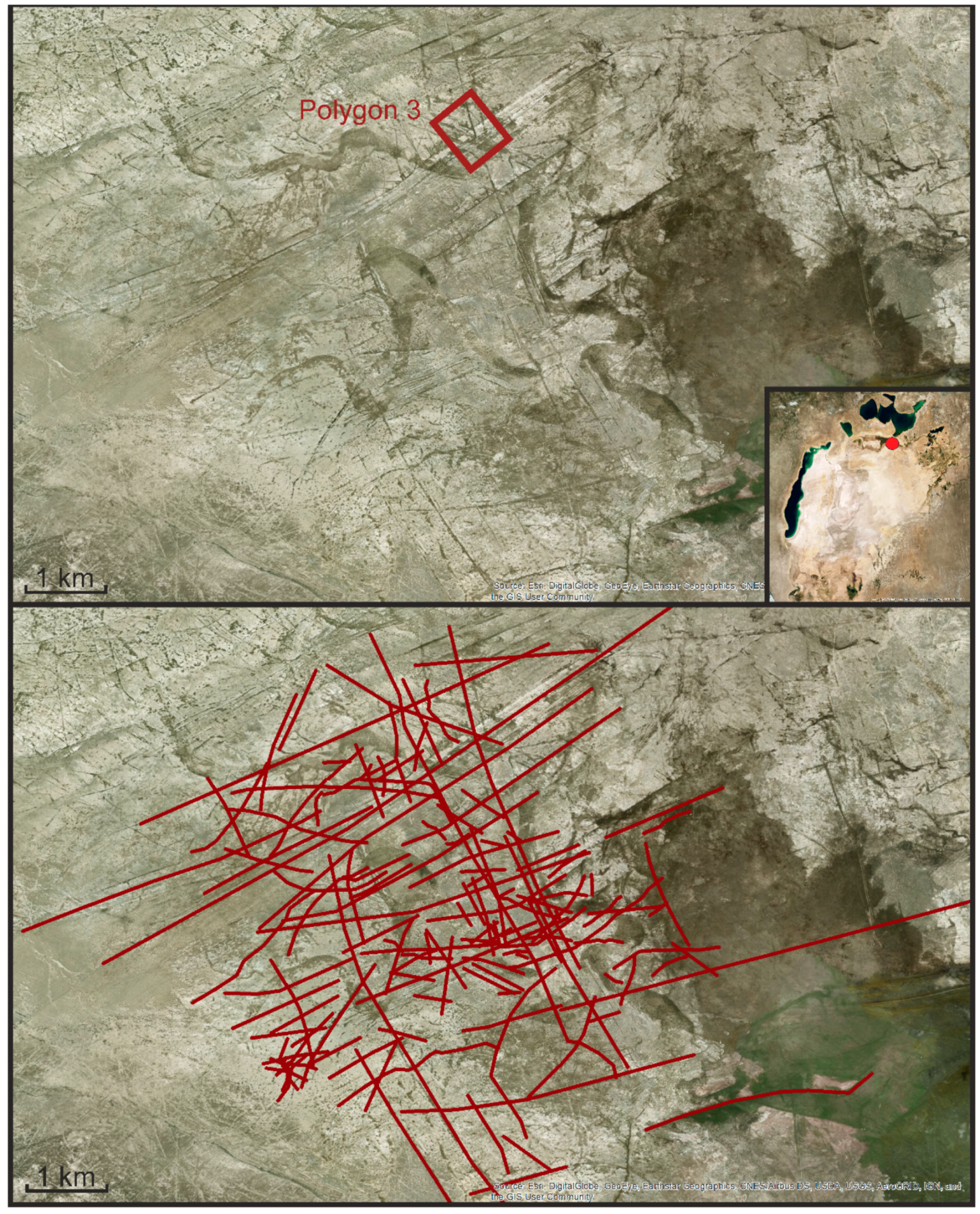
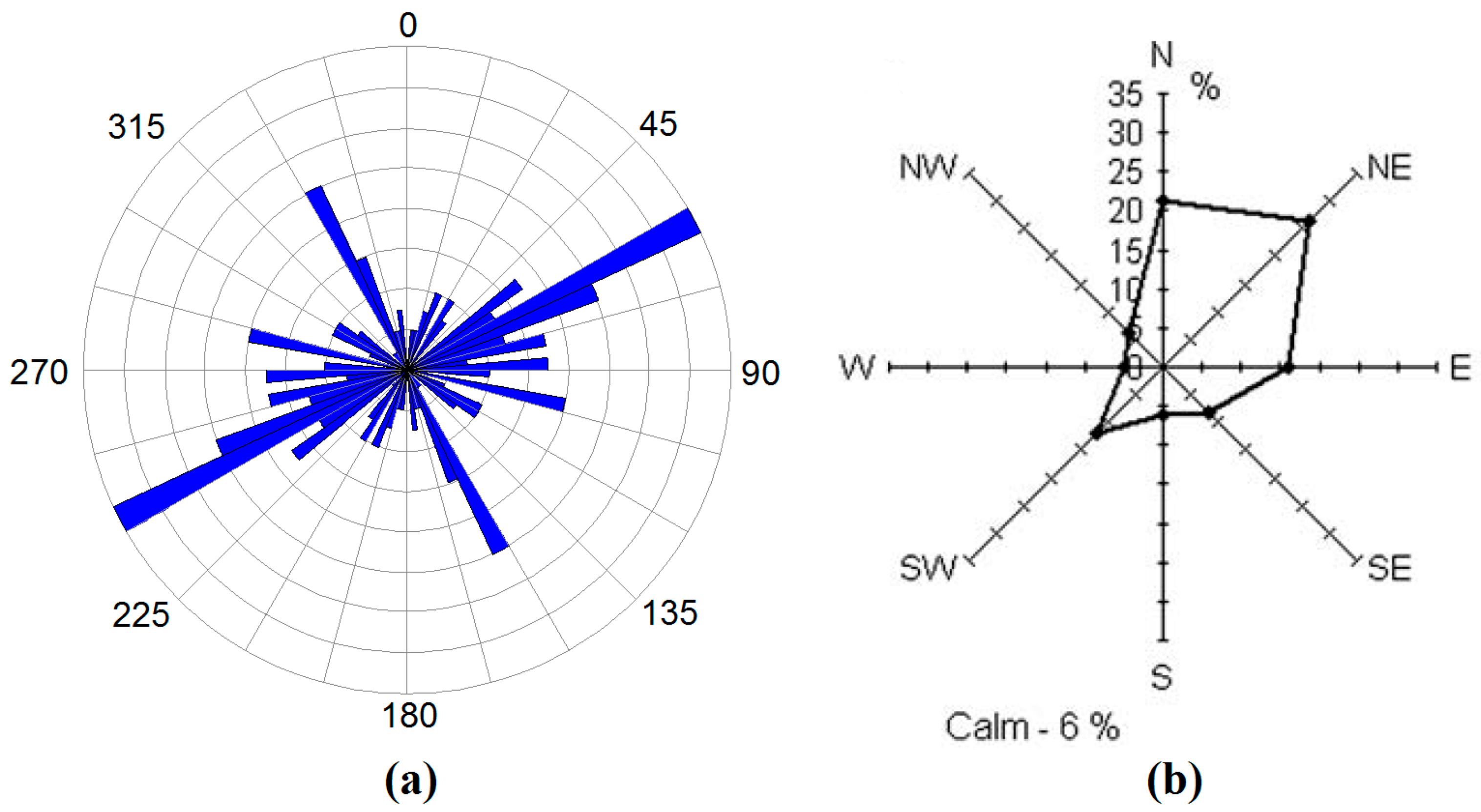
Analysis of satellite imagery of the northeastern Aral Sea has shown abundant linear landforms on the former bottom (Figure 7). Their length varies from hundreds of meters to several kilometers, while their width ranges from 3 m to 90 m (15 m on the average) (Table 2). Numerous “combs”, consisting of several parallel ice scours (four on the average) potentially made by a large ice hummock were discovered. The scours mostly concentrate at former depths from 15 to 25 m in relation to the 53-m a.s.l. base elevation of the lake level before its fall. They have prevailing ENE-WSW (60–240°) directions; maximum secondary peak of the NNW-SSE (150–330°) oriented scours is present (Figure 8). The rose diagram of the scours shows that the orientation of the most abundant scours (first ENE-WSW peak) coincides with the prevailing winds. These scours were created by the drift of large ice bodies pushed by the most frequent winds. The second NNW-SSE direction does not match the distribution of the most frequent winds; however, it is parallel to the coast and fast ice border of the former Aral Sea. These gouges appeared at locations where the ice fields and hummocks collided with stable fast ice, creating scours parallel to its rim. In this way, the orientation of the described scours is typical for linear landforms created by drifting ice and indicates their ice-gouging origin.
About 90% of the scours documented within the study area (northeastern Aral Sea) are straight; 10% are curvilinear. Most of the turns are sharp; however, smooth curves are also observed. The presence of both sharp and smooth bends is a typical feature for ice gouging landforms at the bottom of freezing seas, as the winds pushing the ice formations can change their force and direction either abruptly or slowly, depending on the weather conditions.
In locations with intersections of the scours (Figure 9), they are imposed on each other and cut each other. It can be seen in the figure that scour 1 appeared first and scour 2 crossed it later. Scour 3 cuts both of these scours, being the youngest of the three.
The selected landforms cover most of the study area in the northeast of the Aral Sea; they turned out to be clearly distinguishable both in 2D and 3D by remote-sensing data analysis, UAV investigations and field surveys (Figure 10).
The cross-section of a typical scour consists of two sediment ridges (side berms) divided by a depression stretching over its total length (Figure 10c,d). The depth of the scours varies from 0 to 30 cm, the height of the ridges ranges from 0 to 20 cm, and the total amplitude reaches 50 cm. Field descriptions of the soils in the trial pits and on the surface showed that the ice gouges cut into brownish grey sandy loams (polygon 1), silty loams (polygons 2 and 3) and clayey sands (polygons 4 and 5) with mollusk shells and plant debris. Clayey soils with some sandy particles are typical for the northeastern Aral Sea. For the entire Aral Sea, bottom sediments vary from sands to clays.
Investigations of sections in trial pits showed that sediments in the side berms are looser compared to sediments under the depressions, providing evidence of compaction under pressure along the axis accompanied by mellowing of the berms. In some locations, the ice scours have practically no relief and turn out to be just strips of relatively loose or relatively dense sediments, detectable by the resistance of the soils during excavation, despite the same grain size along the whole profile. The strips of looser and denser sediments also differ in soil color. Due to the lack of vegetation and widespread aeolian processes, ice sours have different preservation and disappear through time. In some areas, e.g., near the former Uzun-Kair Island (northeastern Aral), aeolian deposits cover the ice-gouging landforms completely or partially.
At the ends of the scours, where the hummocks presumably broke off from the bottom, distinctive pressure ridges are seen (Figure 11). Similar forms were found in places where the orientation of a gouge changed as the ice formations were drifting pushed by the changing winds and currents. The pressure ridges are mounds of irregular shape up to 30 cm high, up to 3 m in width.
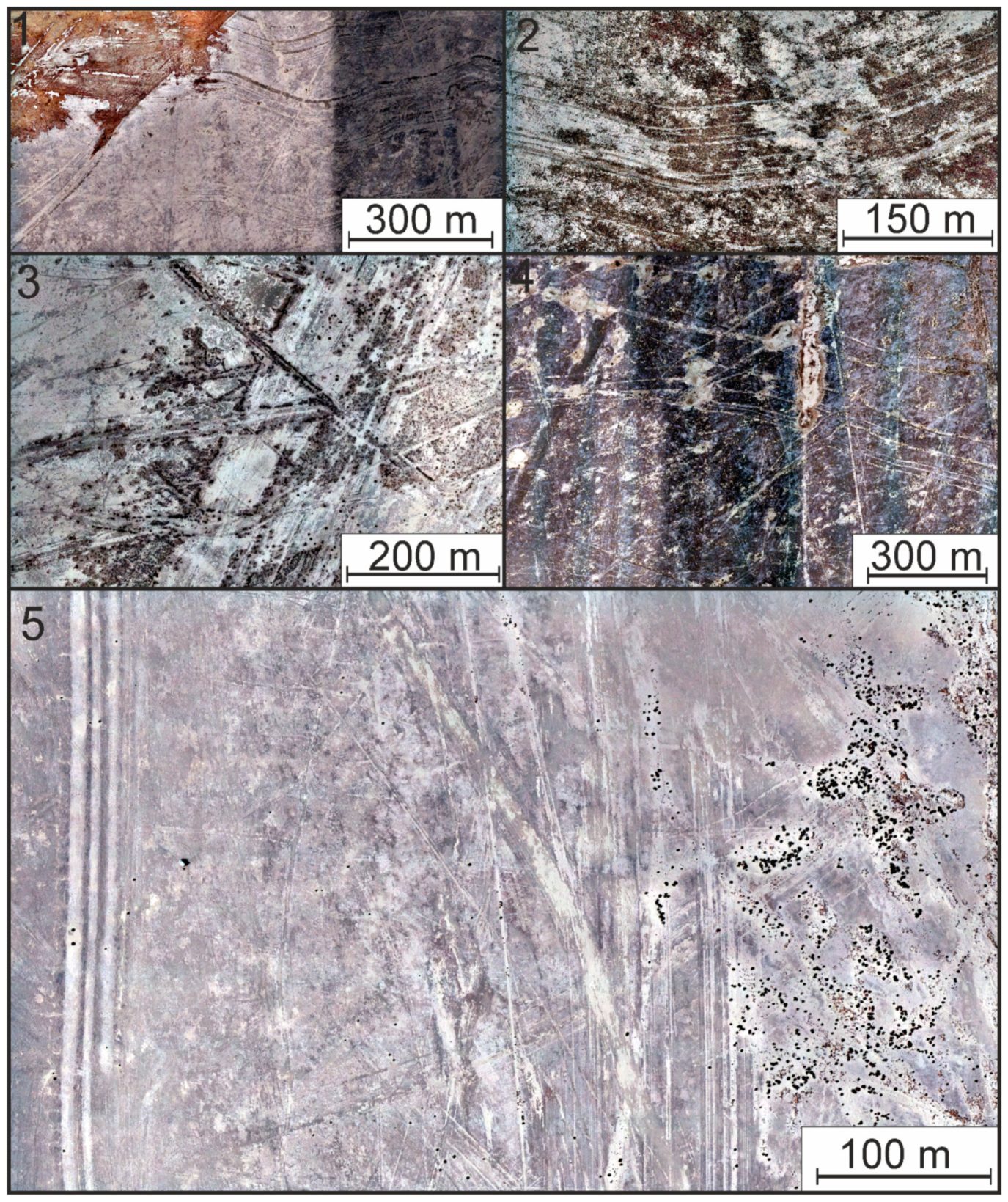
The results of the UAV surveys (Figure 12, Figure 13, Figure 14 and Figure 15) show that the ice scours vary in width and depth. Trenches in the middle have a flat low inclined bottom. On the ortho-photo mosaic, it is seen that shrubs commonly mark side berms and rarely grow in the middle depressions, making deciphering easier. The features of the scours seen on satellite images at smaller scales are similar for smaller ice scours seen by detailed UAV investigations: curves and bends (polygon 1 and 2, Figure 12), presence of multiple parallel scours (all polygons, Figure 12) and overlaying of scours (polygons 1, 3, 4 and 5, Figure 12) are seen in the UAV images.
4.2. Distribution of the Landforms on the Former Aral Sea Bed
The conducted satellite imagery analysis implies that almost the whole former South Aral Sea is covered by the linear landforms which we identify as ice scours. The distribution of their coverage (Figure 16) shows that areas with the highest concentration of ice gouges (more than 50% coverage) are situated in the central part of the East Aral Sea (to the east from the former Barsa-Kelmes Island, Figure 6) and in the southern part of the West Aral Sea, in the vicinity of the remaining reservoir. They occupy about 5% of the whole Aral Sea region. Significant coverage (from 20 to 50%) is typical for areas near the central part of East Aral, to the east of the former Vozrozhdeniya Island and Berg Strait; these areas occupy about 10% of the whole region. The margins of the sea, as a rule, are less covered by the ice gouging landforms (0–20%). At the bottom of the North Aral Sea, ice scours were totally absent.
5. Discussion
5.1. Formation Mechanisms of the Aral Sea Ice-Gouging Topography
The morphology and distribution of the scours derived from satellite imagery and field analysis are in many ways similar to the ice-gouging topography of modern freezing seas and large lakes previously studied by side scan sonar (SSS) surveys [4,52] etc., allowing us to suppose their creation by ice. To prove the origin of the Aral Sea bottom landforms, we compared them to well-studied ice gouges in other seas and lakes. These included the Baydaratskaya Bay of the Kara Sea [53], because of its extensive coverage by SSS data during investigations for construction of an underwater pipeline crossing [4], the northern Caspian Sea [12,19], which is less studied but is proximate to the Aral Sea and has similar conditions, and Lake Erie [23] because of its similar latitudes, water area and conditions.
Identically to ice gouges in these regions, all of the Aral Sea scours have specific morphology with a depression in the axis and parallel side berms, giving evidence of plowing of the bottom ground by ice formations. Relatively dense deposits in the depressions imply pressure of heavy sea ice formations, while looser sediments in the side berms suggest the effect of plowing of the bottom grounds. Both single scours and their combs can be encountered in all freezing seas and lakes ([3], Figure 17). Such combs appear when a grounded hummocky formation or stamukha plows the bottom with its multiple keels. These large ice formations are usually frozen into vast ice floes, increasing their weight and gouging force [54,55]. The larger the ice hummock is, the more keels penetrate into the ground increasing the depth of the scours.
Another feature encountered in the Arctic Seas and in the Caspian and Aral Sea is that both the ice scours and their combs are often imposed (Figure 18) as a result of their consequent formation [3]. One single ice hummock can create numerous scours of different directions cutting each other, as it drifts along the winds and currents.
The scours and ice gouges in all freezing seas, including the former Aral Sea, have bends (Figure 19) which can be both sharp or smooth depending on the rates of the wind direction changes and on the topography of the coastal zone. Stamukha pits, appearing when a large ice hummocky formation (stamukha) is grounded on a shoal and is too heavy for the wind currents to move it, are typical ice gouging landforms as well.
A feature directly evidencing the ice gouging origin of a scour is the presence of front mounds both at the ends of the scours and along their sides (Figure 20). Such mounds, typical for ice gouges of the Caspian and Kara Seas were observed both in field (Figure 10c,d and Figure 12) and by remote sensing at the former Aral Sea bottom.
In addition, the distribution of the scours with their orientation correlating with the directions of the most frequent winds in winter [30], (Figure 8) makes it possible to reliably attribute the gouges of the Aral Sea to traces of ice impact on the bottom.
The morphometric parameters of the scours at the bottom the Aral Sea are also comparable to the dimensions of ice-gouging landforms in other modern freezing seas and lakes (Table 3). The ice gouges of Baydaratskaya Bay are presumably the longest; the SSS surveys showed them to be at least 2 km long; however, parallel surveying lines allow us to suppose much more considerable gouges of several kilometers or even tens of kilometers [4]. Values for the Caspian Sea, Lake Erie and the Aral Sea are comparable, making several kilometers. The Aral Sea ice gouges are wide in relation to other seas and lakes. They are also shallower than the ice gouges of the Caspian Sea, Kara Sea and Lake Erie. Firstly, all of the ice gouges at the Aral Sea were smoothened by waves during the water level decrease, while in all other seas, there are still deep water areas with little wave action and small sedimentation rates, where the scours remain well-preserved. Secondly, after the exposure, aeolian processes contributed to their further filling. Generally, the dimensions of the Aral Sea scours are of the same order as the ice gouging landforms of other freezing seas and lakes.
5.2. Ice-Gouging Intensity Patterns
As seen from Table 3, the average water depths at which the ice scours form vary greatly in different freezing seas and large lakes. On the one hand, the intensity of ice gouging depends on a large array of parameters, being the climate, mechanical properties of ice, bottom topography, etc. On the other hand, conditions of preservation of the scours can be different. As a result, the degree of ice impact does not correlate directly with the number of ice gouges seen on the bottom [3].
Areas close to the coast are usually occupied by fast ice, which moves little and does not form large hummocks; therefore, the forming gouges are small and shallow [1,56]. They are usually destroyed by the first spring storm; therefore, the concentration of ice gouges in coastward regions is usually low. The area with the greatest intensity of ice gouging is the fast ice rim, along which the largest hummocks and ice floes usually drift [14,53]. Deeper water areas are rarely affected, and can be plowed by the largest ice formations only, as their keels have to be very deep to reach the bottom. However, with no wave action and in the absence of currents, the ice scours can be preserved for many years, being repeatedly imposed. After a decade, this will result in high concentrations of gouges, while the ice impact on the bottom in fact occurs rarely.
In this way, the depths of the greatest ice impact vary in different seas, as the zone with the most intense ice action is attributed to the fast ice rim, not to a certain water depth. For Baydaratskaya Bay, Kara Sea, this zone lies at depths between 12 and 26 m [4]. The depths of ice gouging in the American Great Lakes (17–21 m, Table 3) are comparable to the Arctic Seas [23]. In the Caspian Sea, the zone of the most intense ice gouging was proved to appear in shallower water areas at depths of 2–5 m [29].
It has been previously supposed [23] that the depth of ice gouging is mainly controlled by accumulated freezing degree-days (AFDD). At Baydaratskaya Bay, the average air-freezing index calculated in the same way ranged from 3000 to 3500 [57], being the greatest. At the Caspian Sea this value was from 300 to 1300 AFDD [58], being greater than in the region of Lake Erie (285 to 582 AFDD, [23]). At the same time, the depth of ice impact at Lake Erie reaches 25 m [7,23], while the maximum depth of stamukha penetration in the Caspian Sea is 12 m [11] with average values of 2–5 m [29]. The values for the Aral Sea at Barsakelmes Island in its middle part reach 316–1415 AFDD [59], being close to the Caspian Sea values.
The ice thickness does not correlate directly with the depths of impact either: it makes up to 1.2–1.4 m in Baydaratskaya Bay [60], while the average values for Lake Erie and the Caspian Sea are comparable: up to 0.5 m on the average, and never exceeding 0.8 m in Lake Erie [23] and not more than 0.6–0.7 m for drifting ice and 0.9–1.2 m for fast ice in the Northern Caspian Sea [11]. The modern ice thickness varies greatly in the West and the North Aral Sea and depends notably on local conditions; because of the salinity increase, ice thickness in the past should have been greater.
A factor controlling the depth of the greatest ice-gouging intensity might be the bottom topography and inclination of the underwater slopes. Lake Erie and Baydaratskaya Bay are characterized by steeper underwater slopes than the flat Caspian Sea bottom. The floating fast ice has a limited width; at some point it cracks and forms a fissure, along which its rim forms. If, e.g., Lake Erie has steeper underwater slopes than the Caspian Sea, the fast ice rim forming at the same distance from the coast in these two lakes will form at different water depth intervals. Therefore, areas with the most intense ice impact along the rim will be attributed to different depths. The Aral Sea had a very flat bottom in its central and eastern parts, comparable to the Caspian Sea. Therefore, the Northern Caspian Sea can be a model of the past conditions in the Aral Sea. Its extent is comparable to the past area of the Aral Sea; the Southern and Middle Caspian do not freeze and are much deeper, which makes ice gouging impossible. Northerly and northeasterly wind directions prevail in both regions. Moreover, the Caspian Sea and the Aral Sea are situated in similar continental arid desert climate, contrary to the Great American lakes, and experienced considerable water level fluctuations. In this way, we suppose that the patterns of ice impact in the past at the Aral Sea were comparable to the modern Northern Caspian Sea, with depths of the most intense ice gouging along the fast ice rim at 2–5 m. In the nearshore zone with 1–2 m depths, fast ice should have been stable and hummocking was not intensive. At depths of more than 6 m, hummocky formations were presumably not thick enough for their keels to penetrate into the ground.
The preservation of the ice scours at freezing seas is generally controlled by the wave base, which, in its turn, is influenced by the wind fetch, the size of the lake or sea and wind direction. Wave action could not be great at the Aral Sea. The winds blow from land both in winter and in summer and rarely affect the northeastern coast. As the wave base is close to the sea depth, the waves lose their energy, not reaching the nearshore zone. In the conditions of water level decrease, the depth of wave impact was controlled by the vast shallows, limiting sediment transport. This confirms the absence of scours to the northeast from the Vozrozhdeniya Island, and abundant scours to the southwest from it, in the wind shadow.
At the same time, unlike the Caspian Sea and at the Arctic seas, the distribution of ice scours at the Aral Sea bottom was influenced by another factor, absent elsewhere: its dramatic and rapid water level drop. While it could not affect the density of the ice scours, it promoted their unprecedented preservation. In one year, the coastline could retreat by several kilometers, and therefore the wave action did not have time to destroy the ice scours. The density of the scours, in turn, was more influenced by the local bottom topography and the width of the water surface affecting the acceleration of ice floes and the formation of hummocks. In this way, while the intensity of ice scouring can be compared to the Arctic seas and to the Caspian Sea, the coverage of the bottom by scours is in some way a snapshot showing both old ice scours with good preservation and young scours which formed in one winter that would otherwise have been destroyed by waves.
This unique snapshot setting raises the interest in complementary simultaneous studies of the Northern Caspian and Aral Seas. Because of their comparable climate, the mechanisms and patterns of sea ice effect should have been similar in the past. Today, the Northern Caspian still represents conditions typical for the Aral Sea several decades ago. Its ice gouging landforms are seen on the remotely sensed images only immediately after the water area becomes clear of ice (Figure 21). Then, they are eroded by the first spring storms. As the studies of parameters and distribution of such forms are constrained by their short lifetime, good preservation of ice gouges at the silty Aral Sea bottom ground after the level drop allows us to investigate similar landforms and extend the results to the Northern Caspian.
At the same time, while today conditions in the Aral Sea are not favorable for ice gouging, there is a possibility to reconstruct such past conditions by observing modern sea ice and analyzing different ice phenomena in the Caspian Sea (Figure 22). Similarly to the modern Northern Caspian, in the Aral Sea, multiple ice floes collided under the wind force, forming ice ridges that could affect the bottom. Stamukhas were breaking off the ice cover and contributing to the new hummocking. In this way, the Caspian Sea provides an opportunity for investigations of ice conditions, mechanisms and processes of ice gouging, while at the Aral Sea, the results of such processes can be documented. Further comprehensive studies of the two seas could add to our understanding of the ice-gouging processes in the mid-latitude climates.
In this way, the distribution of the scours in the Aral Sea and their density patterns (Figure 16) are a result of both the varying ice-gouging intensity and the different degree of their preservation. The spatially non-uniform intensity of ice impact resulted in lower concentrations of ice scours in the coastward parts, while in the central part, there were more ice gouges, just as in Baydaratskaya Bay [4] and the Caspian Sea [63]. The largest coverage of the central part of the Eastern Aral Sea by scours was also provided by their long-term accumulation when the water level was at 2–5 m above vast flat bottom plains in its center. Moreover, a fast water level drop promoted the preservation of bottom fragments with high ice scour concentrations even in relatively shallow areas. Despite the northerly and northeasterly winds, which pushed the ice to the south in the Caspian and Aral Sea, most of the Aral Sea ice gouges are concentrated in its flat central part. On the one hand, the southern coasts were protected by the fast ice. On the other hand, the coastline retreated faster in the north and east, while in the south, water remained until the 2000s. Therefore, old ice gouges from the 1990s remained in the central and eastern part, and were destroyed by waves in the south. Younger ice gouges from the 2000s were less abundant as the air and water temperatures increased, along with the salinity; the ice formations became smaller and could execute less impact on the bottom.
At the North Aral Sea, the small size of the water area, insufficient to speed up drifting ice and hummocks, and its complete freezing every year limited ice gouging. The West Aral Sea could not provide favorable conditions for ice gouging because of its high salinity and steep nearshore bottom slopes. Therefore, there are no ice gouges neither at the North Aral Sea nor near the western coast of the West Aral Sea.
5.3. Temporal Evolution of the Aral Sea Ice-Gouging Topography
Knowing the position of the retracting Aral Sea shoreline in space and time [40] (Figure 16), and assuming that the most intense ice impact is typical for depths of 2–5 m, similarly to the Northern Caspian, we were able to reconstruct the history of the ice-gouging topography at the Aral Sea bottom. Based on the known rates of lake level fluctuation, the formation time of separate scours can be estimated. We suggest that most of them formed along with the rapid sea-level fall of 1980–mid-1990s when the depth interval of 2–5 m at the East Aral generally shifted westwards along with the coastline. During this whole level fall, the zone of intense ice impact moved from depths of about 15–18 m to 22–25 m in relation to the 53-m base elevation. The rate of water level drop (reaching 70 cm per year from the mid-1970s to the early 1990s) was so high that the ice scours could not be filled with the bottom sediments. In one year, several kilometers of the former bottom surface became exposed, providing an unprecedented degree of ice-gouging topography preservation.
In the mid-1990s and 2000s, the shallowing slowed down, and extensive shoals formed. At that time, vast areas were in conditions favorable for ice gouging (2–5 m depths). At the same time, the wave action on the east coast was almost absent due to its flat topography, small depths and prevalence of storm winds blowing from the northeast. In the late 2000s, the waters of the East Aral Sea became hypersaline, and the ice formation diminished. The surface area of the sea reduced to such an extent that rare ice could not get enough acceleration for the hummocking. The ice-gouging processes, therefore, largely ceased.
Today, ice gouging is almost absent at the Aral Sea. The East Aral Sea, which used to be the area with the most intense ice impact, has now entirely dried out. In the West Aral Sea, the water is hypersaline, and ice forms at extremely low temperatures; it is thin and incapable of plowing the bottom. On the North Aral Sea, ice gouging is limited, as it always was. Today, no significant regional climate or anthropogenic drivers can cause an increase of the Aral Sea level [64], so it is unlikely that the ice effect on the bottom will intensify in the nearest future.
6. Conclusions
At the bottom of the former Aral Sea, exposed after a dramatic man-induced fall in water level, linear landforms were recently discovered [28,63]. Their analysis using remote-sensing and field (UAV and geomorphological) methods has shown that the landforms range from 3 to 90 m width (15 m on the average), from 100 m to several km length (1 km on the average) and have a depth of up to 0.5 m. Areas with their greatest density are situated in the central part of the former East Aral Sea.
The forms were proved to be ice gouges and scours made by drifting ice during higher water level position in the past. We have shown that the climate of the Aral Sea region provided favorable conditions for ice scouring of the bottom by hummocks both before and during the water level fall. The directions of the scours correspond to the most frequent winds in the cold season. Their morphology, morphometry and distribution are typical for ice scours, known in the Arctic, Caspian and other freezing seas and large lakes. Just as with the ice scours of the Caspian Sea, Kara Sea and other freezing seas, the gouges of the Aral Sea have a trench in the middle surrounded by ridges; they make both sharp and smooth bends and curves; they are often juxtaposed; front mounds are documented at their ends.
The evolution of the ice impact on the Aral Sea bottom was determined by changes of the lake level since the 1960s. The most intense ice gouging happened in the 1980s–mid-1990s, when the zone of the greatest impact (2–5 m depths) shifted from 15–18 to 22–25 m a.s.l. In the 1990s–2000s, the shallowing slowed down, and ice scours continued to form at extensive shoals. In the late 2000s, ice gouging ceased as a result of salinity increase and water area decrease; it is unlikely to intensify in the nearest future.
The Aral Sea represents a unique setting for studies of ice-gouging topography. No other present or former water body provides such vast areas of exposed bottom with scours that are relatively easy to access. Due to a very rapid water level fall, good preservation of ice scours became possible. On the exposed bottom of the Aral Sea, we can see a snapshot of gouges that formed during a single season and areas with the results of repeated impact.
Author Contributions
S.M. Aral Sea geomorphology field data, remote-sensing data interpretation, paper writing and preparation; S.O. project administration, conceptualization, supervision, funding acquisition, review and editing; A.B. conceptualization, review and editing, paper writing (Discussion and Conclusions); A.V. photogrammetric field data and its processing, visualization; V.A. Baydaratskaya Bay field data; P.B. Caspian Sea field data.
Funding
This research was funded by the Russian Science Foundation, grant number 16–17-00034.
Acknowledgments
We are very grateful to Egor Zelenin (Geological Institute, Russian Academy of Science), Leonid Ostroumov, Igor Zemlianov, Alexander Tsvetsinsky (Zubov State Oceanographic Institute) and Alexander Izhitskiy (Shirshov Institute of Oceanology, Russian Academy of Science) for providing field equipment and support.
Conflicts of Interest
The authors declare no conflict of interest.
References
- Barnes, P.W.; Rearic, D.M.; Reimnitz, E. Ice gouging characteristics and processes. In The Alaskan Beaufort Sea: Ecosystems and Environments; Barnes, P.W., Schell, D.M., Reimnitz, E., Eds.; Academic Press Inc.: Orlando, FL, USA, 1984; pp. 185–212. [Google Scholar]
- Forbes, D.L.; Taylor, R.B. Ice in the shore zone and the geomorphology of cold coasts. Prog. Phys. Geogr. 1994, 18, 59–89. [Google Scholar] [CrossRef]
- Ogorodov, S.A. The Role of Sea Ice in Coastal Dynamics; MSU Publishers: Moscow, Russia, 2011; p. 173. ISBN 978-5-211-06275-7. (In Russian) [Google Scholar]
- Ogorodov, S.A.; Arkhipov, V.V.; Kokin, O.V.; Marchenko, A.; Overduin, P.; Forbes, D. Ice effect on coast and seabed in Baydaratskaya Bay, Kara Sea. Geogr. Environ. Sustain. 2013, 3, 32–50. [Google Scholar]
- Rex, R.W. Microrelief produced by sea ice grounding in the Chukchi Sea near Barrow, Alaska. Arctic 1955, 8, 177–186. [Google Scholar] [CrossRef]
- Reimnitz, E.; Barnes, P.W.; Forgatsch, Т.; Rodeick, C. Influence of grounding ice on the Arctic shelf of Alaska. Mar. Geol. 1972, 13, 323–334. [Google Scholar] [CrossRef]
- Grass, J.D. Ice scour and ice ridging studies in Lake Erie. In Proceedings of the 7th International Symposium on Ice, Hamburg, Germany, 27–31 August 1984; International Association of Hydraulic Engineering and Research: Hamburg, Germany, 1984. [Google Scholar]
- Forbes, D.L.; Manson, G.K.; Chagnon, R.; Solomon, S.M.; van der Sanden, J.J.; Lynds, T.L. Nearshore ice and climate change in the southern Gulf of St. Lawrence. In Ice in the Environment, Proceedings of the 16th International Symposium on Ice, Dunedin, New Zealand, 2–6 December 2002; International Association of Hydraulic Engineering and Research: Beijing, China, 2002. [Google Scholar]
- Vershinin, S.A.; Truskov, P.A.; Kuzmichev, K.V. Ice Effect on the Constructions at Sakhalin Shelf; Giprostroymost Institute: Moscow, Russia, 2005; p. 208. (In Russian) [Google Scholar]
- Koshechkin, B.I. Traces of the moving ice on the bottom surface of shallow water areas of the Northern Caspian. Proc. Airborne Methods Lab. AS USSR 1958, 6, 227–234. (In Russian) [Google Scholar]
- Bukharitsin, P.I. Dangerous hydrological phenomena on the Northern Caspian. Water Resour. 1984, 21, 444–452. (In Russian) [Google Scholar]
- Ogorodov, S.A.; Arkhipov, V.V. Caspian Sea Bottom Scouring by Hummocky Ice Formations. Doklady Earth Sci. 2010, 432, 703–707. [Google Scholar] [CrossRef]
- Fuglem, M.; Parr, G.; Jordaan, I.; Verlaan, P.; Peek, R. Sea Ice Scour Depth and Width Parameters for Design of Pipelines in the Caspian Sea. In Proceedings of the 22nd International Conference on Port and Ocean Engineering under Arctic Conditions, Espoo, Finland, 9–13 June 2013; Curran Associates, Inc.: Red Hook, NY, USA, 2014. [Google Scholar]
- Hnatiuk, J.; Brown, K. Sea bottom scouring in the Canadian Beaufort Sea. In Proceedings of the 9th Annual Offshore Technology Conference, Houston, TX, USA, 2–5 May 1977. [Google Scholar]
- Liferov, P.; Shkhinek, K.N.; Vitali, L.; Serre, N. Ice gouging study—Actions and action effects. In Recent Development of Offshore Engineering in Cold Regions, Proceedings of 19th International Conference on Port and Ocean Engineering under Arctic Conditions, Dalian, China, 27–30 June 2007; Yue, Q., Ji, S., Eds.; Dalian University of Technology Press: Dalian, China, 2007. [Google Scholar]
- Løset, S.; Shkhinek, K.N.; Gudmestad, O.T.; Høyland, K.V. Actions from Ice on Arctic Offshore and Coastal Structures; LAN: St. Petersburg, Russia, 2006; p. 271. ISBN 5-8114-0703-3. [Google Scholar]
- Barrette, P. Offshore pipeline protection against seabed gouging by ice: An overview. Cold. Reg. Sci. Technol. 2011, 69, 3–20. [Google Scholar] [CrossRef]
- Lanan, G.A.; Cowin, T.G.; Johnston, D.K. Alaskan Beaufort Sea pipeline design, installation and operation. In Proceedings of the Arctic Technology Conference, Houston, TX, USA, 7–9 February 2011; Curran: Red Hook, NY, USA, 2011. [Google Scholar]
- Bukharitsin, P.I.; Ogorodov, S.A.; Arkhipov, V.V. The impact of floes on the seabed of the northern Caspian under the conditions of sea level and ice cover changes. Vestnik Moskovskogo Universiteta Seriya 5 Geografiya 2015, 2, 101–108. (In Russian) [Google Scholar]
- Langlois, T.H.; Langlois, M.H. The ice of Lake Erie around South Bass Island 1936–1964. In Center for Lake Erie Research; Technical Report No. 165, Book Series; Ohio State University College of Biological Sciences: Columbus, OH, USA, 1985; p. 172. [Google Scholar]
- Gilbert, R.; Glew, J.R. A wind driven ice push event in eastern Lake Ontario. J. Great Lakes Res. 1987, 2, 326–331. [Google Scholar] [CrossRef]
- Bolsenga, S.J. A Review of Great Lakes Ice Research. J. Great Lakes Res. 1992, 18, 169–189. [Google Scholar] [CrossRef]
- Daly, S.F. Characterization of the Lake Erie Ice Cover; U.S. Army Engineer Research and Development Center (ERDC), Cold Regions Research and Engineering Laboratory (CRREL): Hanover, NH, USA, 2016; p. 100. [Google Scholar]
- Gilbert, R.; Handford, K.J.; Shaw, J. Ice Scours in the Sediments of Glacial Lake Iroquois, Prince Edward County, Eastern Ontario. Geogr. Phys. Quat. 1992, 46, 189–194. [Google Scholar] [CrossRef] [Green Version]
- Eden, D.J. Ice Scouring as a Geologic Agent: Pleistocene Examples from Scarborough Bluffs and a Numerical Model. Master's Thesis, University of Toronto, Toronto, ON, Canada, 2000. [Google Scholar]
- Eyles, N.; Meulendyk, T. Ground-penetrating radar study of Pleistocene ice scours on a glaciolacustrine sequence boundary. Boreas 2008, 37, 226–233. [Google Scholar] [CrossRef]
- Lorenz, R.D.; Jackson, B.K.; Barnes, J.W.; Spitale, J.; Keller, J.M. Ice rafts not sails: Floating the rocks at Racetrack Playa. Am. J. Phys. 2011, 79, 37–42. [Google Scholar] [CrossRef]
- Smerdov, B.A. Traces on the Aral Sea Bottom. 2008. Available online: http://cetext.ru/b-a-smerdov-sledi-na-dne-araleskogo-morya-nauchnoe-issledovani.html (accessed on 12 November 2018).
- Maznev, S.V.; Ogorodov, S.A. Ice scours on the exposed bottom of the Aral Sea. In Proceedings of the 18th International Multidisciplinary Scientific GeoConference SGEM 2018, Albena, Bulgaria, 2–8 July 2018; STEF92 Technology Ltd.: Sophia, Bulgaria, 2018. [Google Scholar]
- Kostianoy, A.G.; Kosarev, A.N. The Aral Sea Environment. The Handbook of Environmental Chemistry; Springer-Verlag: Berlin/Heidelberg, Germany, 2010; Volume 7, p. 335. ISBN 978-3-540-88276-3. [Google Scholar]
- Zavialov, P.O. Physical Oceanography of the Dying Aral Sea; Springer, Praxis Publishing Ltd.: Chichester, UK, 2005; p. 154. ISBN 3-540-22891-8. [Google Scholar]
- Bortnik, V.N.; Chistiaeva, S.P. Hydrometeorology and Hydrochemistry of USSR’s Seas, Vol. 7: Aral Sea; Gidrometeoizdat: Leningrad, Russia, 1990; p. 195. ISBN 5-286-00746-5. (In Russian) [Google Scholar]
- Aral Sea (North) | General Info | Database for Hydrological Time Series of Inland Waters (DAHITI). Available online: https://dahiti.dgfi.tum.de/en/81/ (accessed on 12 November 2018).
- Aral Sea (East) | General Info | Database for Hydrological Time Series of Inland Waters (DAHITI). Available online: https://dahiti.dgfi.tum.de/en/82/ (accessed on 12 November 2018).
- Aral Sea (West) | General Info | Database for Hydrological Time Series of Inland Waters (DAHITI). Available online: https://dahiti.dgfi.tum.de/en/83/ (accessed on 12 November 2018).
- INTAS Project—0511 REBASOWS. Final Report: The Rehabilitation of the Ecosystem and Bioproductivity of the Aral Sea under Conditions of Water Scarcity; IWHW-BOKU: Vienna, Austria; Tashkent, Uzbekistan, 2006; p. 276. [Google Scholar]
- Zavialov, P.O.; Arashkevich, E.G.; Bastida, I.; Ginzburg, A.I.; Dikaryov, S.N.; Zhitina, L.S.; Izhitsky, A.S.; Ishniyazov, D.P.; Kostyanoy, A.G.; Kravtsova, V.I.; et al. Big Aral Sea in Early XXI Cent.: Physics, Biology, Chemistry; Science: Moscow, Russia, 2012; p. 227. ISBN 978-5-02-037987-9. (In Russian) [Google Scholar]
- Kosarev, A.N. Hydrology of the Caspian and Aral Seas; MSU Publishers: Moscow, Russia, 1975; p. 252. (In Russian) [Google Scholar]
- Mikhailov, V.N.; Kravtsova, V.I.; Gurov, F.N.; Markov, D.V.; Grégoire, M. Assessment of the present-day state of the Aral Sea. Vestnik Moskovskogo Univ. Seriya 5 Geogr. 2001, 6, 14–21. (In Russian) [Google Scholar]
- Ginzburg, A.I.; Kostianoy, A.G.; Sheremet, N.A.; Kravtsova, V.I. Satellite monitoring of the Aral Sea. Ecol. Monit. Ecosyst. Model. Probl. 2010, XXIII, 150–193. (In Russian) [Google Scholar]
- Kouraev, A.V.; Kostianoy, A.G.; Lebedev, S.A. Ice cover and sea level of the Aral Sea from satellite altimetry and radiometry (1992–2006). J. Mar. Syst. 2009, 76, 272–286. [Google Scholar] [CrossRef]
- World Imagery—ArcGIS Online. Available online: https://www.arcgis.com/home/item.html?id=10df2279f9684e4a9f6a7f08febac2a9 (accessed on 12 November 2018).
- Bing Maps—Directions, Trip Planning, Traffic Cameras & More. Available online: https://www.bing.com/maps (accessed on 12 November 2018).
- Yandex Maps. Available online: https://yandex.ru/maps/ (accessed on 12 November 2018).
- Google Maps. Available online: https://www.google.ru/maps (accessed on 12 November 2018).
- User Manual DJI. Available online: https://dl.djicdn.com/downloads/phantom_4_pro/Phantom+4+Pro+Pro+Plus+User+Manual+v1.0.pdf (accessed on 12 November 2018).
- Getting Started and Manual—Pix4D Support. Available online: https://support.pix4d.com/hc/en-us/sections/200733429-Getting-Started-and-Manual (accessed on 12 November 2018).
- Agisoft PhotoScan. Available online: http://www.agisoft.com/ (accessed on 12 November 2018).
- Koci, J.; Jarihani, B.; Leon, J.X.; Sidle, R.C.; Wilkinson, S.N.; Bartley, N. Assessment of UAV and Ground-Based Structure from Motion with Multi-View Stereo Photogrammetry in a Gullied Savanna Catchment. Int. J. Geo-Inf. 2017, 6, 328. [Google Scholar] [CrossRef]
- Smith, M.W.; Carrivick, J.L.; Quincey, D.J. Structure from motion photogrammetry in physical geography. Prog. Phys. Geogr. 2016, 40, 247–275. [Google Scholar] [CrossRef]
- Eltner, A.; Kaiser, A.; Castillo, C.; Rock, G.; Neugirg, F.; Abellán, A. Image-based surface reconstruction in geomorphometry—Merits, limits and developments. Earth Surf. Dyn. 2016, 4, 359–389. [Google Scholar] [CrossRef]
- Bryant, R.S. Side Scan Sonar for Hydrography—An Evaluation by the Canadian Hydrographic Service. Int. Hydrogr. Rev. 1975, 52, 43–56. [Google Scholar]
- Ogorodov, S.A.; Arkhipov, V.V.; Baranskaya, A.V.; Kokin, O.V.; Romanov, A.O. The influence of climate change on the intensity of ice gouging of the bottom by hummocky formations. Doklady Earth Sci. 2018, 478, 228–231. [Google Scholar] [CrossRef]
- Yang, Q.S.; Poorooshasb, H.B. Numerical Modeling of Seabed Ice Scour. Comput. Geotech. 1997, 21, 1–20. [Google Scholar] [CrossRef]
- Marchenko, A.V.; Ogorodov, S.A.; Shestov, A.S.; Tsvetsinsky, A.S. Ice gouging in Baidaratskaya bay of the Kara Sea: Field studies and numerical simulations. In Proceedings of the International Conference on Port and Ocean Engineering under Arctic Conditions, Dalian, China, 27–30 June 2007; Yue, Q., Ji, S., Eds.; Dalian University of Technology Press: Dalian, China, 2007. [Google Scholar]
- Reimnitz, E.; Barnes, P.W. Sea ice as a geologic agent on the Beaufort Sea shelf of Alaska. In The Coast and Shelf of the Beaufort Sea; Reed, J.C., Sater, J.E., Eds.; Arctic Institute of North America: Arlington, TX, USA, 1974; pp. 301–353. [Google Scholar]
- Shabanova, N.; Ogorodov, S.; Shabanov, P.; Baranskaya, A. Hydrometeorological forcing of western Russian Arctic coastal dynamics: XX-century history and current state. Geogr. Environ. Sustain. 2018, 11, 113–129. [Google Scholar] [CrossRef]
- Ivkina, N.; Naurozbaeva, Z.; Clove, B. Impact of climate change on the Caspian Sea ice regime. Cent. Asian J. Water Res. 2017, 3, 15. Available online: https://www.water-ca.org/article/2589 (accessed on 12 November 2018). (In Russian).
- Temnikov, S.N. Ice coverage and winters’ asperity at the Aral Sea. In Lakes and Water Storage Reservoirs of the Central Asia: Proceedings of SARNIGMI; Ivanov, Y.N., Nikitin, A.M., Eds.; Gidrometeoizdat: Moscow, Russia, 1979; pp. 75–81. (In Russian) [Google Scholar]
- Bogorodsky, P.V.; Marchenko, A.V.; Pniushkov, A.V. Aspects of fast ice forming in nearshore zone of freezing seas. Arctic Antarct. Res. 2007, 77, 17–27. (In Russian) [Google Scholar]
- Landsat Image Gallery—Ice Scours the North Caspian Sea. Available online: https://landsat.visibleearth.nasa.gov/view.php?id=87903 (accessed on 12 November 2018).
- Grounded in Caspian Sea. Available online: https://earthobservatory.nasa.gov/images/89742/grounded-in-the-caspian-sea (accessed on 12 November 2018).
- Ogorodov, S.A. Ice gouging topography at the bottom of Caspian and Aral seas. In Proceedings of the Thirteenth International MEDCOAST Congress on Coastal and Marine Sciences, Engineering, Management and Conservation, Mellieha, Malta, 31 October–4 November 2017; Ozhan, E., Ed.; Mediterranean Coastal Foundation Dalyan: Mugla, Turkey, 2017. [Google Scholar]
- Micklin, P. The future Aral Sea: Hope and despair. Environ. Earth Sci. 2016, 75, 9. [Google Scholar] [CrossRef]
Figure 1.
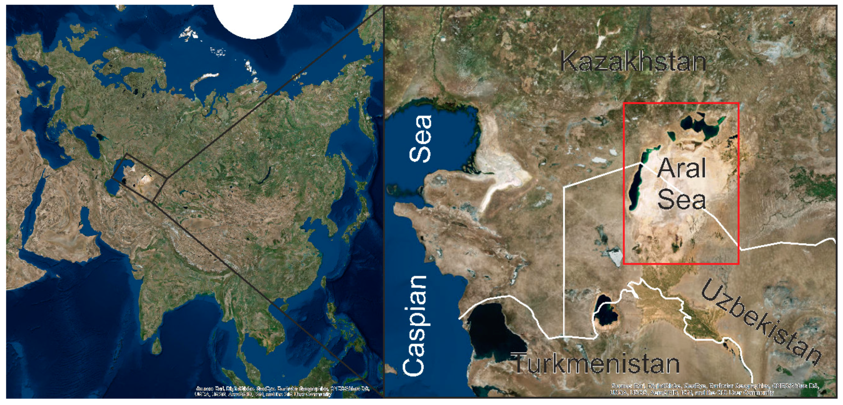
Study area. The red rectangle surrounds the territory of the Aral Sea during its greatest extent in the 20th century.
Figure 1.
Study area. The red rectangle surrounds the territory of the Aral Sea during its greatest extent in the 20th century.

Figure 2.
Bathymetric chart of the Aral Sea referenced to a pre-1960 water level (53 m a.s.l.) [36].
Figure 2.
Bathymetric chart of the Aral Sea referenced to a pre-1960 water level (53 m a.s.l.) [36].

Figure 3.
Fluctuations of the Aral Sea level (after [30]–before 1993 and after [33,34,35]–in 1993–2018). 1–Aral Sea (1960–1986); 2–North Aral Sea (1986–2018); 3–South Aral Sea (1986–2006); 4–East Aral Sea (2007–2018); 5–West Aral Sea (2007–2018).
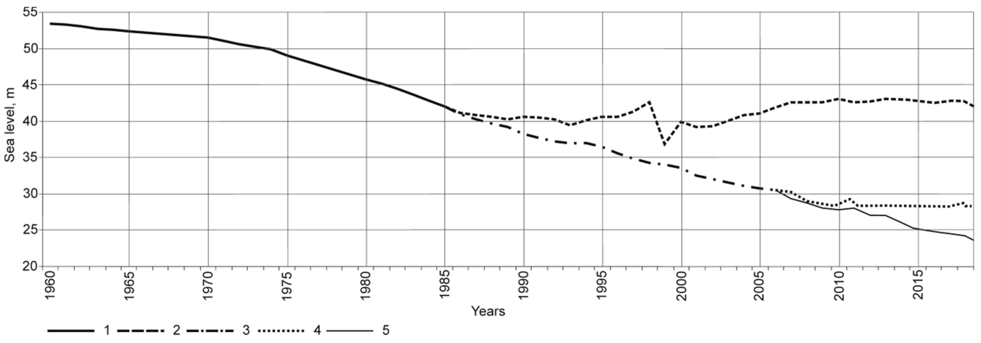
Figure 4.
General view of the exposed Aral Sea bottom; key sites of fieldwork are shown by red dots; hydrometeorological stations are shown by blue rectangles; the red line indicates the coastline in 1960 and shows the area where ice scours were deciphered for estimations of their density. Background: ESRI, DigitalGlobe (WorldView-2).
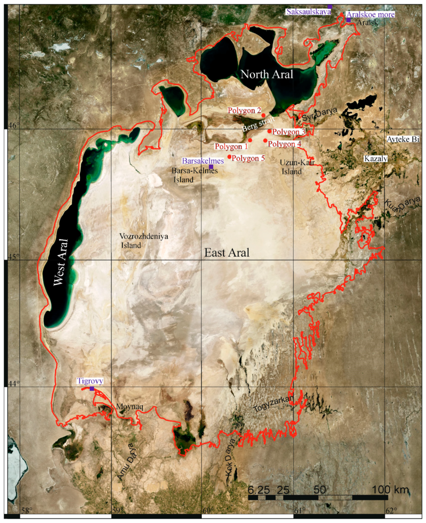
Figure 5.
Frequency of wind directions (%) at the hydrometeorological station (HMS) Aralskoe More (Aral Sea), (a) in February, (b) annual, (c) mean monthly wind velocities (ms−1) [30], locations of HMSs are given in Figure 4.

Figure 6.
Fragment of WorldView-3 [42] space image showing significant coverage of the former bottom by scours to the west of Barsa-Kelmes Island.
Figure 6.
Fragment of WorldView-3 [42] space image showing significant coverage of the former bottom by scours to the west of Barsa-Kelmes Island.
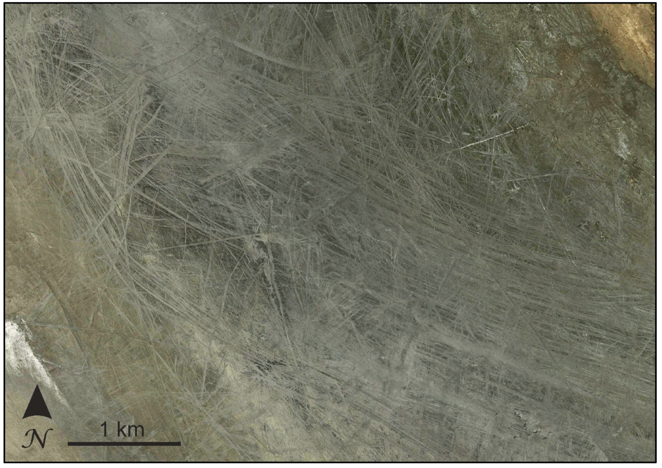
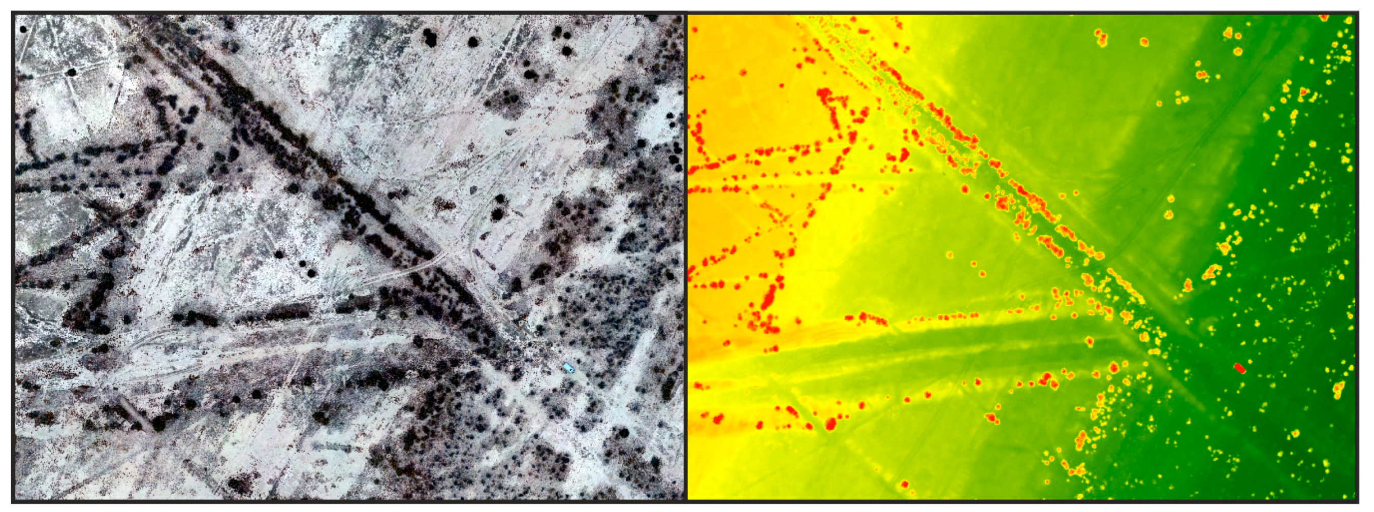
Figure 7.
Example of imagery interpretation: initial space image (top) and interpretation scheme (bottom). The location of the area is shown as a red dot.
Figure 7.
Example of imagery interpretation: initial space image (top) and interpretation scheme (bottom). The location of the area is shown as a red dot.

Figure 8.
Rose diagrams showing the prevailing directions of scours at the northeastern Aral Sea (a); frequency of wind directions (%), for February (b).
Figure 8.
Rose diagrams showing the prevailing directions of scours at the northeastern Aral Sea (a); frequency of wind directions (%), for February (b).

Figure 9.
Overlapping of the scours on the Aral Sea bottom from UAV survey (polygon 3). Scour 1 is the oldest, scour 2 is younger, scour 3 is the youngest.
Figure 9.
Overlapping of the scours on the Aral Sea bottom from UAV survey (polygon 3). Scour 1 is the oldest, scour 2 is younger, scour 3 is the youngest.
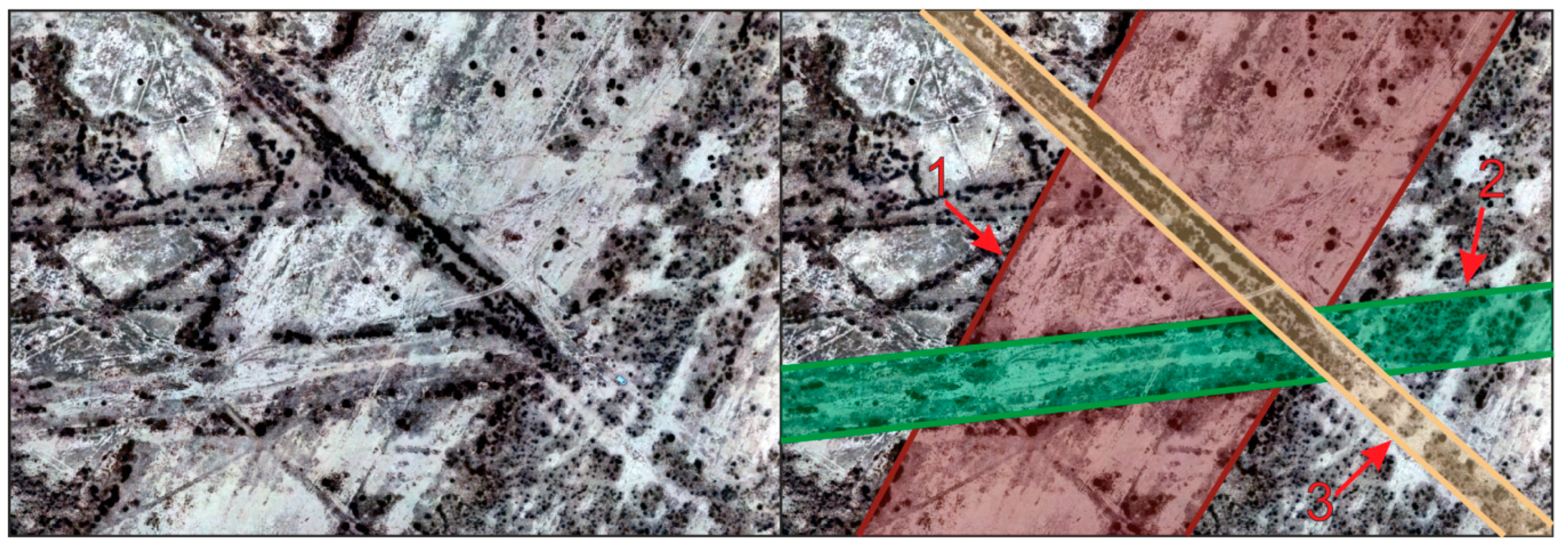
Figure 10.
View of a model ice scour: (polygon 3): (a) on space imagery (WorldView-3) [42]; (b) on the ortho-photo mosaic (UAV survey); (c) ground view; (d) cross-section taken from a leveling survey. The location of the place where the ground view photo was taken is shown as a red pointer; the red line AB indicates the position of the leveling profile.
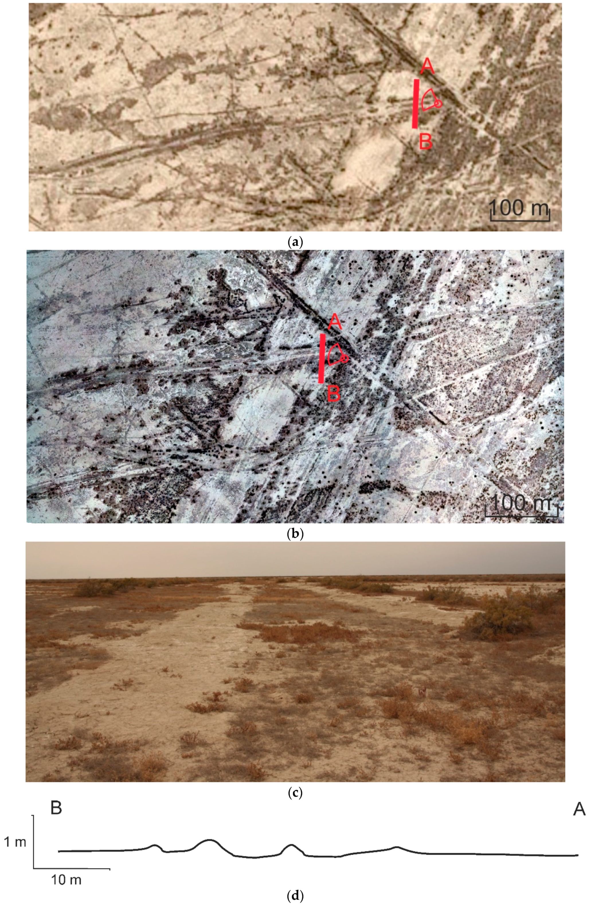
Figure 11.
An example of a ground (left) and aerial (right) view of small pressure ridges at polygon 2.
Figure 11.
An example of a ground (left) and aerial (right) view of small pressure ridges at polygon 2.
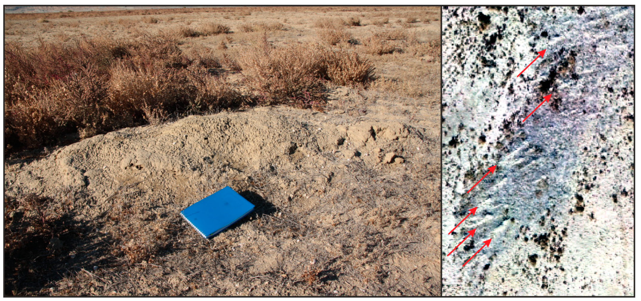
Figure 12.
Results of the UAV survey in the northeast of the Aral Sea. The number in the left top corner corresponds to the number of the polygon in Figure 4.
Figure 12.
Results of the UAV survey in the northeast of the Aral Sea. The number in the left top corner corresponds to the number of the polygon in Figure 4.

Figure 13.
A fragment of the ortho-photo mosaic (left) and preliminary digital elevation model (DEM) (right) of polygon 3. Colors of the DEM show lower (green, 36 m a.s.l.) and higher (red, 37 m a.s.l.) elevations.
Figure 13.
A fragment of the ortho-photo mosaic (left) and preliminary digital elevation model (DEM) (right) of polygon 3. Colors of the DEM show lower (green, 36 m a.s.l.) and higher (red, 37 m a.s.l.) elevations.

Figure 14.
A fragment of the ortho-photo mosaic (left) and preliminary DEM (right) of the northern part of polygon 5. Colors of the DEM show lower (green, 34 m a.s.l.) and higher (red, 35 m a.s.l.) elevations.
Figure 14.
A fragment of the ortho-photo mosaic (left) and preliminary DEM (right) of the northern part of polygon 5. Colors of the DEM show lower (green, 34 m a.s.l.) and higher (red, 35 m a.s.l.) elevations.
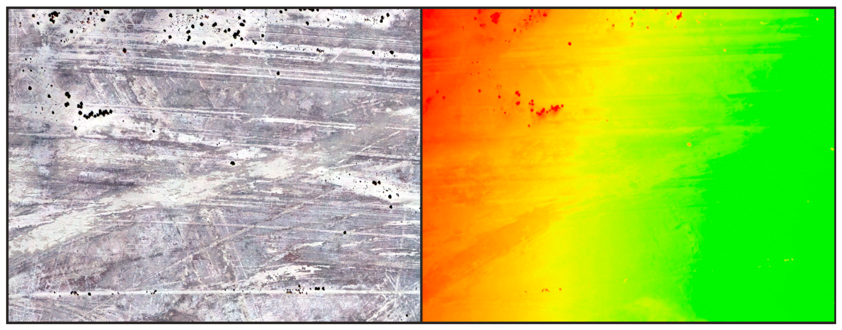
Figure 15.
A fragment of the ortho-photo mosaic (left) and preliminary DEM (right) of the southern part of polygon 5. Colors of the DEM show lower (green, 34 m a.s.l.) and higher (red, 35 m a.s.l.) elevations.
Figure 15.
A fragment of the ortho-photo mosaic (left) and preliminary DEM (right) of the southern part of polygon 5. Colors of the DEM show lower (green, 34 m a.s.l.) and higher (red, 35 m a.s.l.) elevations.
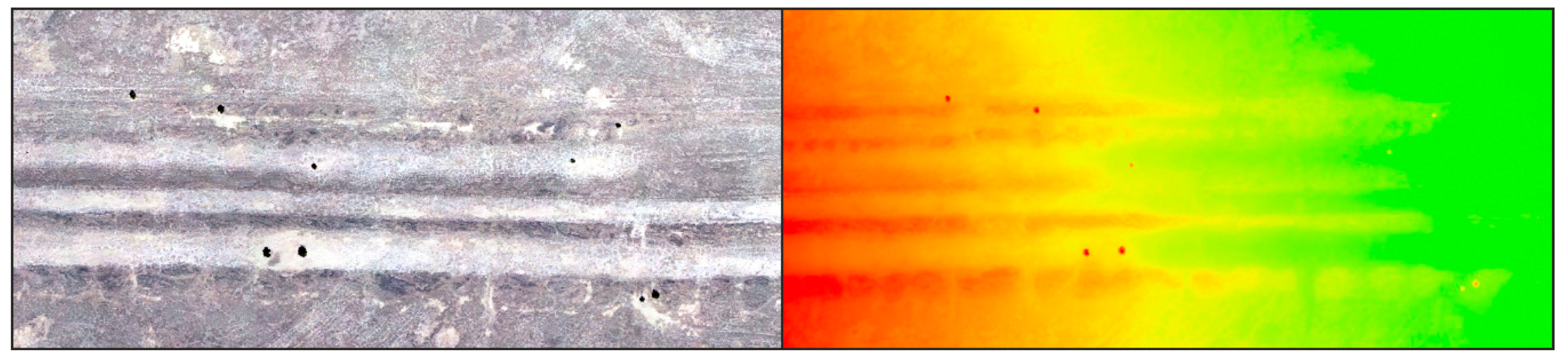
Figure 16.
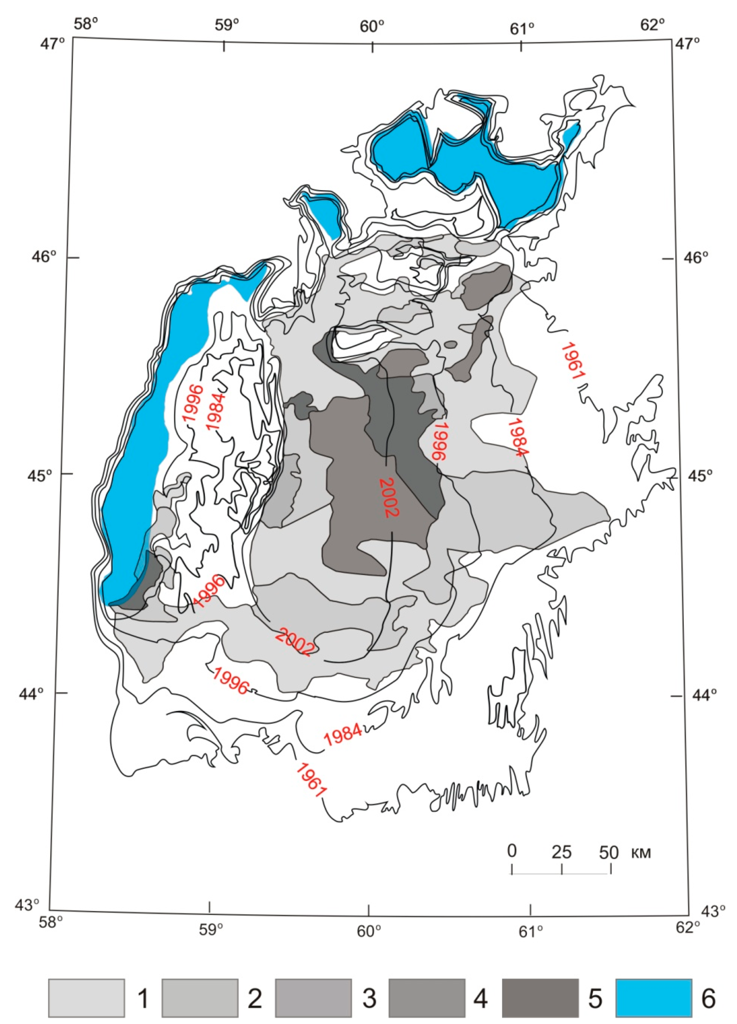
Estimated coverage of the Aral Sea bottom by ice scours: (1) <10% of ice scour coverage, (2) 10–20%, (3) 20–30%, (4) 30–50%, (5) >50%, (6) modern Aral Sea water area. Background: contours of the former shorelines after [40].
Figure 16.
Estimated coverage of the Aral Sea bottom by ice scours: (1) <10% of ice scour coverage, (2) 10–20%, (3) 20–30%, (4) 30–50%, (5) >50%, (6) modern Aral Sea water area. Background: contours of the former shorelines after [40].

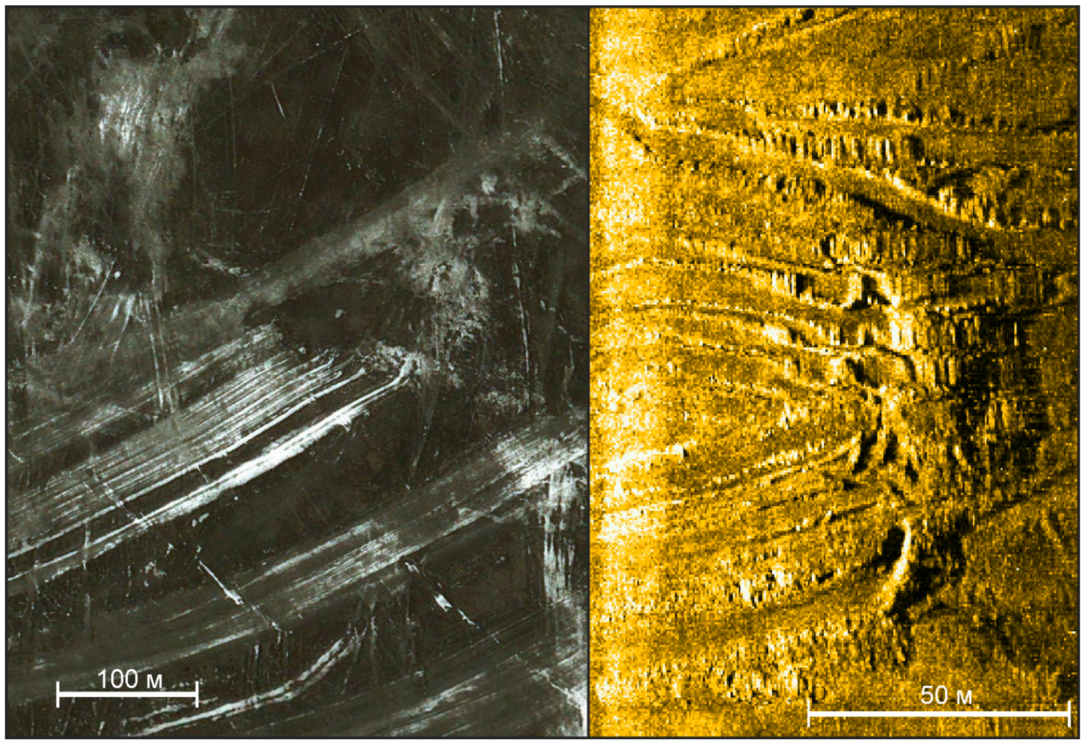
Figure 17.
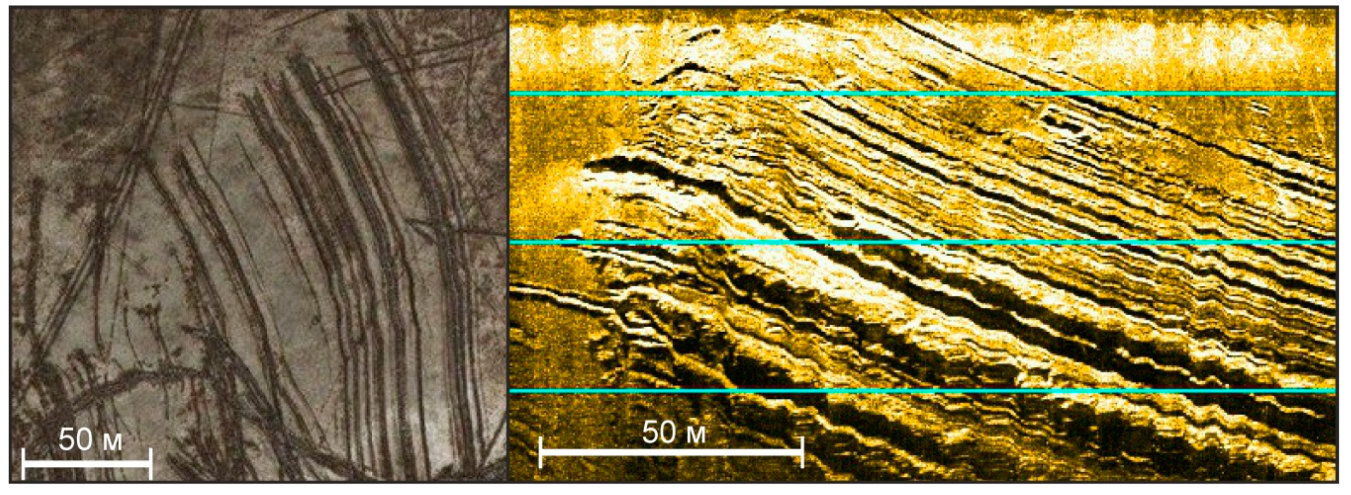
“Combs” of ice scours at the bottom of the Aral Sea (WorldView-3, left) [42] and at the bottom of the Baydaratskaya Bay (side scan sonar (SSS) survey, right).
Figure 17.
“Combs” of ice scours at the bottom of the Aral Sea (WorldView-3, left) [42] and at the bottom of the Baydaratskaya Bay (side scan sonar (SSS) survey, right).

Figure 18.
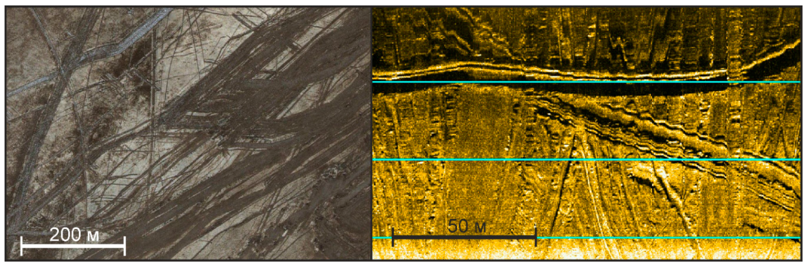
Imposition of ice gouging “combs” at the bottom of the Aral Sea (WorldView-3, left) [42] and at the bottom of the Baydaratskaya Bay (SSS survey, right).
Figure 18.
Imposition of ice gouging “combs” at the bottom of the Aral Sea (WorldView-3, left) [42] and at the bottom of the Baydaratskaya Bay (SSS survey, right).

Figure 19.
Bending ice scours at the bottom of the Aral Sea (WorldView-3, left) [42] and at the bottom of the Baydaratskaya Bay (SSS survey, right).
Figure 19.
Bending ice scours at the bottom of the Aral Sea (WorldView-3, left) [42] and at the bottom of the Baydaratskaya Bay (SSS survey, right).
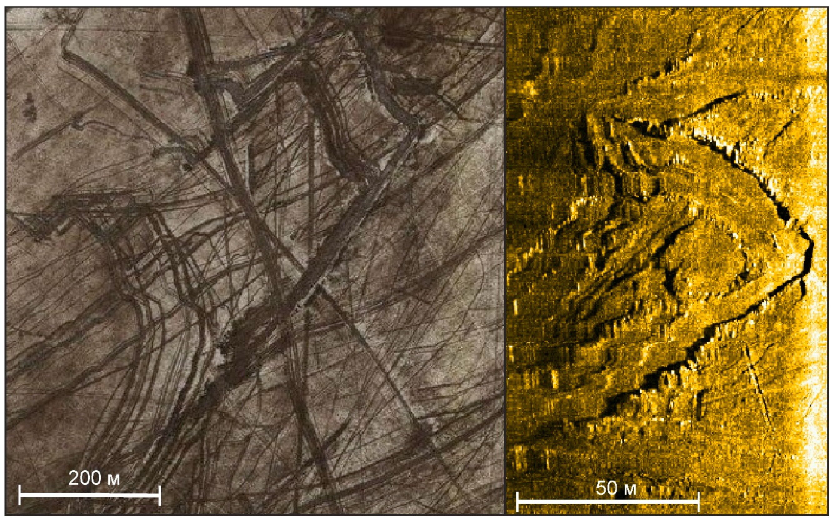
Figure 20.
Front mounds at the ends of the “combs” at the bottom of the Aral Sea (WorldView-3, left) [42] and at the bottom of the Baydaratskaya Bay (SSS survey, right).
Figure 20.
Front mounds at the ends of the “combs” at the bottom of the Aral Sea (WorldView-3, left) [42] and at the bottom of the Baydaratskaya Bay (SSS survey, right).

Figure 21.
Ice scours on the Northern Caspian Sea bottom, Tyuleniy Archipelago (acquired 16 April 2016) [61].
Figure 21.
Ice scours on the Northern Caspian Sea bottom, Tyuleniy Archipelago (acquired 16 April 2016) [61].
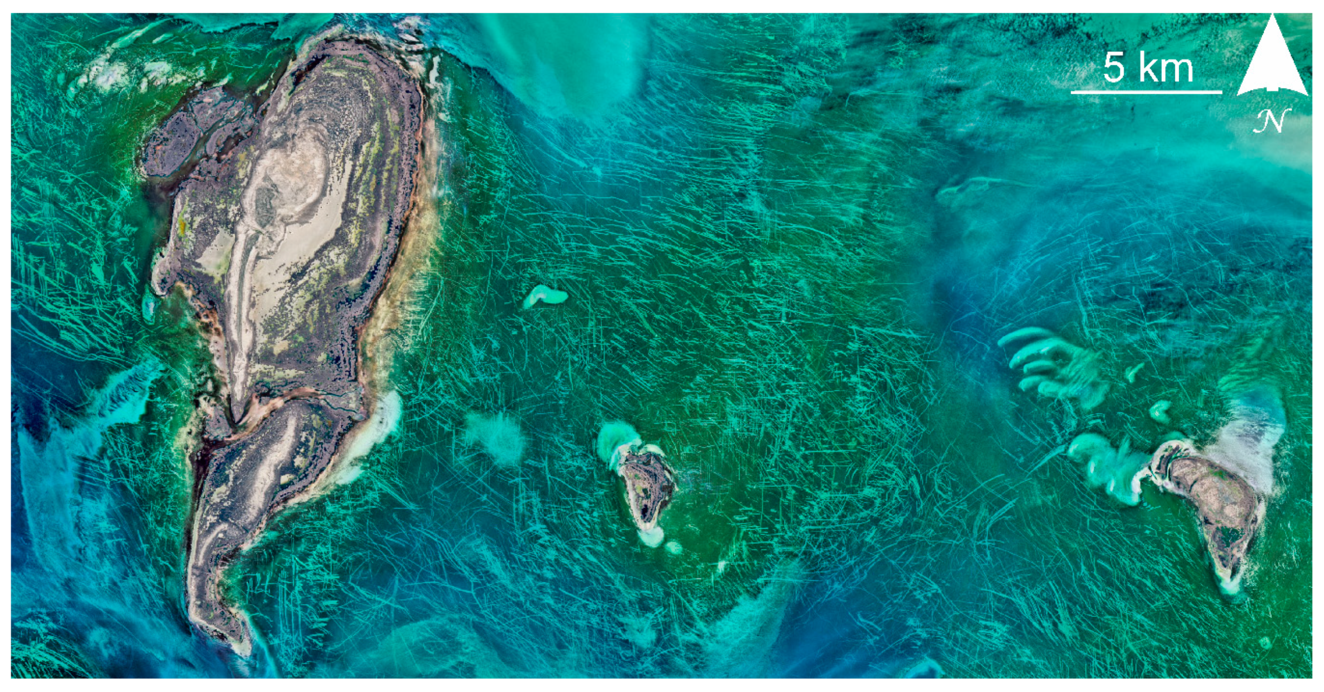
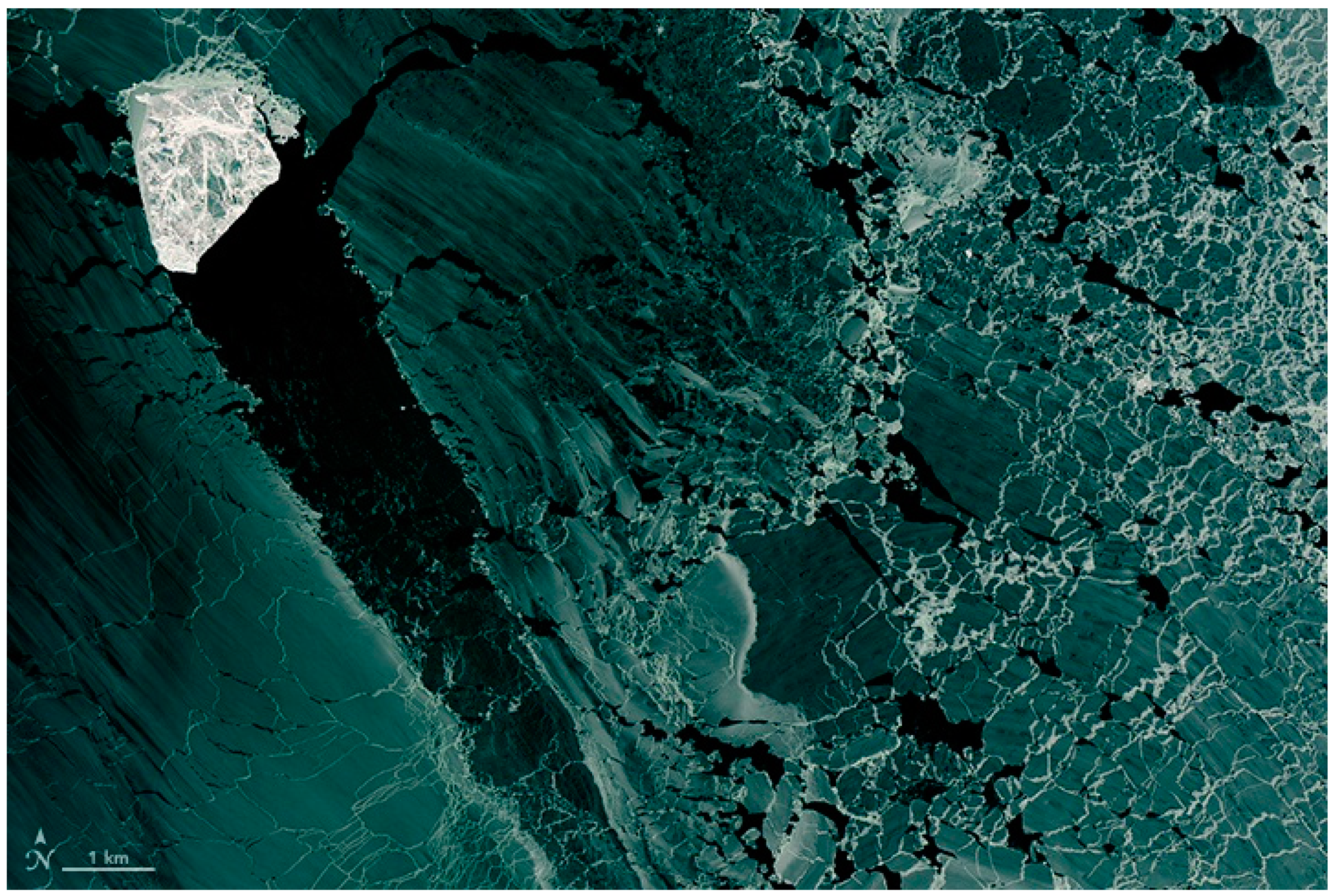
Figure 22.
Ice conditions at the Northern Caspian Sea on 4 February 2017 [62]. Ice hummock (stamukha) grounded on the seabed and open water trace behind it.
Figure 22.
Ice conditions at the Northern Caspian Sea on 4 February 2017 [62]. Ice hummock (stamukha) grounded on the seabed and open water trace behind it.


Table 1.
Parameters of the unmanned aerial vehicle (UAV) survey.
| Survey Height, m | Frame Length, m | Frame Width, m | Resolution, m Per Pixel | Vertical Accuracy, m |
|---|---|---|---|---|
| 100 | 125 | 70 | 0.025 | 0.04 |
| 50 | 50 | 30 | 0.01 | 0.04 |
Table 2.
Parameters of the ice scours of the northeastern Aral Sea bottom.
| Characteristic | Length, m | Single Scour Width (with Ridges), m | Comb Width, m |
|---|---|---|---|
| Minimum | 106 | 3 | 13 |
| Maximum | 8650 | 89 | 386 |
| Average | 1302 | 15 | 72 |
Table 3.
Comparison of ice scours of the Aral, Caspian, and Kara Seas and Lake Erie.
| Sea | Average Length | Average Width, m | Average Depth of an Ice Scour, m | Average Water Depth of the Ice Scours’ Formation, m | Preservation Time |
|---|---|---|---|---|---|
| Aral Sea | 1300 m | 15 | 0.2 | 2–5 (assumption) | decades |
| Caspian Sea [19,29] | several km | 5 | 1.0 | 2–5 | few months |
| Kara Sea (Baydaratskaya Bay) [4] | several km | 10 | 1.0 | 12–26 | from 1–2 years to few decades |
| Lake Erie [23] | 4.5–6.0 km | 60–100 | >1.0 | 17–21 | ? |
© 2019 by the authors. Licensee MDPI, Basel, Switzerland. This article is an open access article distributed under the terms and conditions of the Creative Commons Attribution (CC BY) license (http://creativecommons.org/licenses/by/4.0/).
Share and Cite
MDPI and ACS Style
Maznev, S.; Ogorodov, S.; Baranskaya, A.; Vergun, A.; Arkhipov, V.; Bukharitsin, P. Ice-Gouging Topography of the Exposed Aral Sea Bed. Remote Sens. 2019, 11, 113. https://0-doi-org.brum.beds.ac.uk/10.3390/rs11020113
AMA Style
Maznev S, Ogorodov S, Baranskaya A, Vergun A, Arkhipov V, Bukharitsin P. Ice-Gouging Topography of the Exposed Aral Sea Bed. Remote Sensing. 2019; 11(2):113. https://0-doi-org.brum.beds.ac.uk/10.3390/rs11020113
Chicago/Turabian StyleMaznev, Stepan, Stanislav Ogorodov, Alisa Baranskaya, Aleksey Vergun, Vasiliy Arkhipov, and Peter Bukharitsin. 2019. "Ice-Gouging Topography of the Exposed Aral Sea Bed" Remote Sensing 11, no. 2: 113. https://0-doi-org.brum.beds.ac.uk/10.3390/rs11020113
Note that from the first issue of 2016, this journal uses article numbers instead of page numbers. See further details here.