A Novel FPGA-Based Architecture for Fast Automatic Target Detection in Hyperspectral Images

 , ,
, , 
Abstract
:1. Introduction
- A solution is derived to remove traditional complex inversion in ATGP-OSP by a simple method. The proposed method is capable of achieving real-time detection without sacrificing target quality at a fixed scale of operation.
- A novel effectively update structure for orthogonal projection operator is proposed to accelerate Fast-ATGP. A normalized vector is adopted to replace the classical operator to complete the projection process.
- The proposed architecture can greatly balance speedup factors and resources by combining the serial-parallel structure and multiplex technique, which is optimal for processing wealthy HSI information in terms of real-time hardware implementation.
- The approach can be simply reconstructed by adjusting several parameters in HLS. As a consequence, the framework is able to support HSI with different sizes and spectral bands and conforms to multiple amounts of processing element (PE) to achieve different levels of parallelism.
2. Background
2.1. ATGP-OSP Algorithm
| Algorithm 1 Pseudocode of ATGP-OSP |
| 1: Inputs: , and t; % denotes an n-dimensional hyperspectral image with r pixels, and t denotes the number of targets to be detected 2: ; % is the initial target signature with maximum length in 3: for to do 4: ; % is a vector orthogonal to the subspace spanned by the columns of 5: ; % is projected onto the direction indicates by 6: ; % The maximum projection value is found, where r denotes the total number of pixel in the hyperspectral image and the operator “:” denotes “all elements” 7: ; % The target matrix is updated 8: end for i 9: Outputs: ; |
2.2. Analysis
2.2.1. Increasing Operation Problem
2.2.2. Huge Matrix Multiplication Problem
3. The Proposed Approach
| Algorithm 2 Pseudocode of Fast-ATGP |
| 1: Input: , and t; % denotes an n-dimensional hyperspectral image with r pixels and t denotes the number of targets to be detected 2: Initialized: , , ; % is the identity matrix and L denotes spectral bands of HSI, and are the initialized orthogonal projection operators 3: for to do 4: ; % HSI data is projected onto the direction indicates by 5: ; % The maximum projection value is found, where r denotes the total number of pixels 6: ; % The target is detected and the target matrix is updated, where the operator “:” denotes “all elements” 7: % , used for updating the operator and , is a vector obtained by the target signature projected onto the direction indicated by 8: % The projection operator of matrix is updated 9: ; % The projection operator of vector is updated 10: end for i 11: Output: ; |
3.1. The Principle of Fast-ATGP
3.1.1. Fixed Scale of Operation
3.1.2. Update Operator in One Step
3.2. Parallel Strategy
- (1)
- The master divides the HSI data into spatial-domain partitions according to the number of PEs, and sends partitions and operator to all parallel processing units.
- (2)
- Each processing unit finds the pixel vector with maximum length in its local partition. Specifically, performing the dot-product operation in step 4 of Algorithm 2, and completing the comparison and target selection process in step 5 of Algorithm 2. It is worth noting that the above two steps can be implemented using HLS in parallel. In other words, the local brightest pixel vector can be selected while operating dot-product simultaneously. Then, each unit sends the spatial location and maximum length of the pixel to master respectively.
- (3)
- The master finds the global pixel vector () with the maximum length. Then, the pixel vector is serially projected into the orthogonal subspace (step 7 of Algorithm 2). Finally, the master updates the orthogonal projection operators and , and broadcasts to all units.
- (4)
- Repeat from step 2 to step 3 until a set of t target pixels are extracted from the original cube.
4. FPGA Implementation
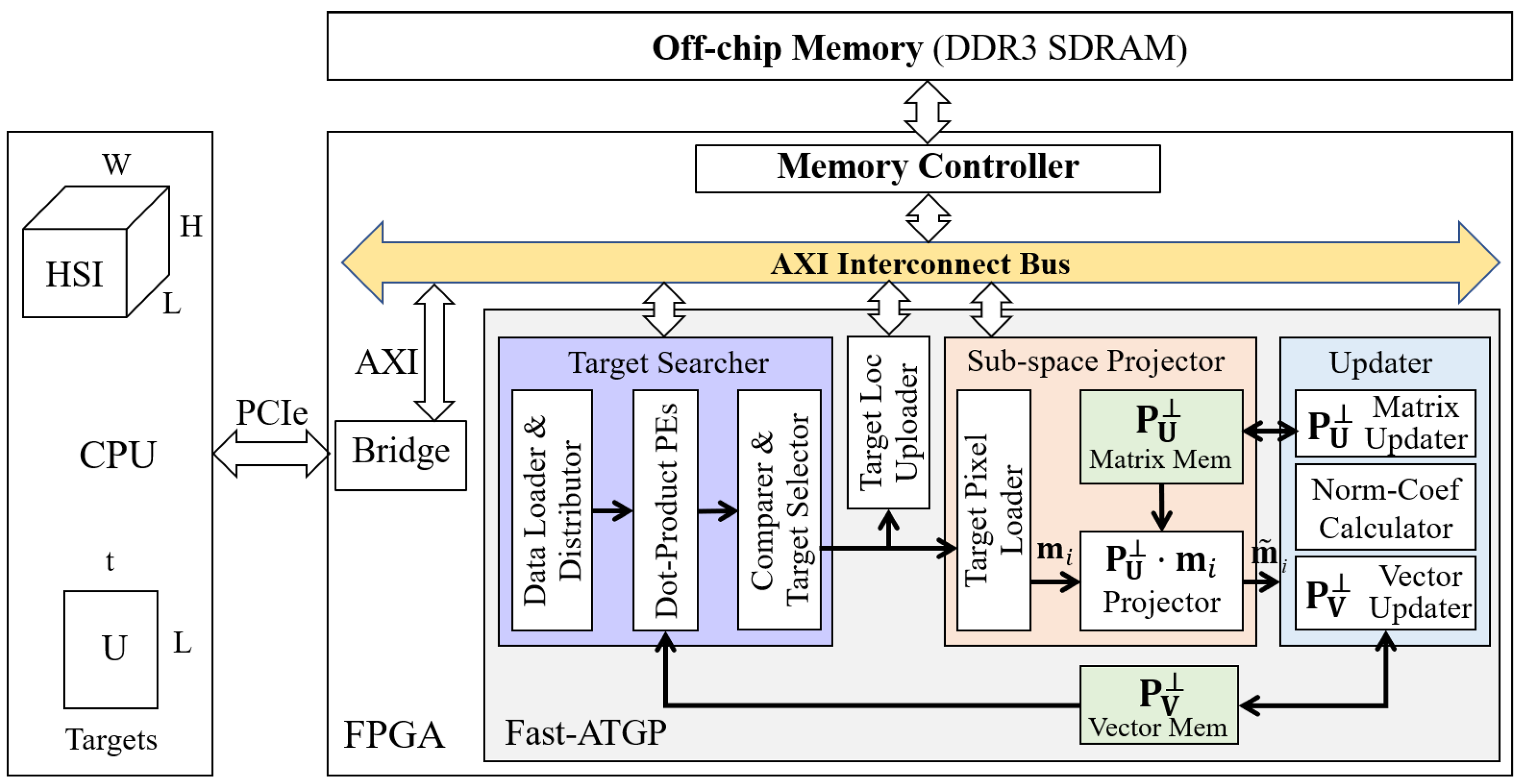
4.1. Overall Hardware Architecture of Fast-ATGP
4.2. Microscopic Hardware Architecture of Fast-ATGP
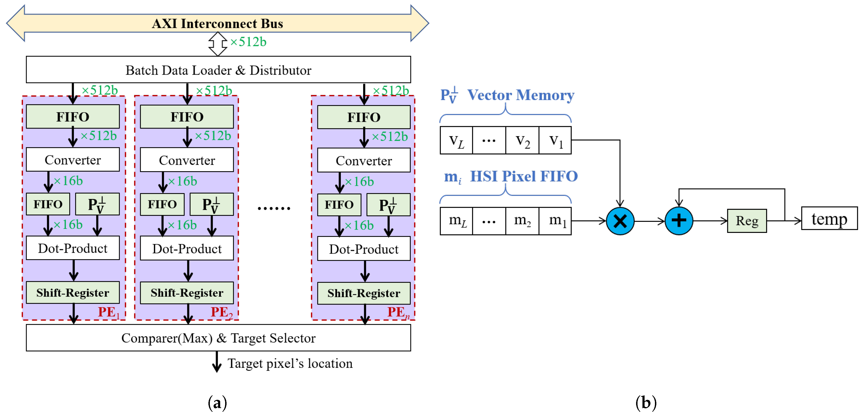
4.2.1. Target Searcher
4.2.2. Sub-Space Projector
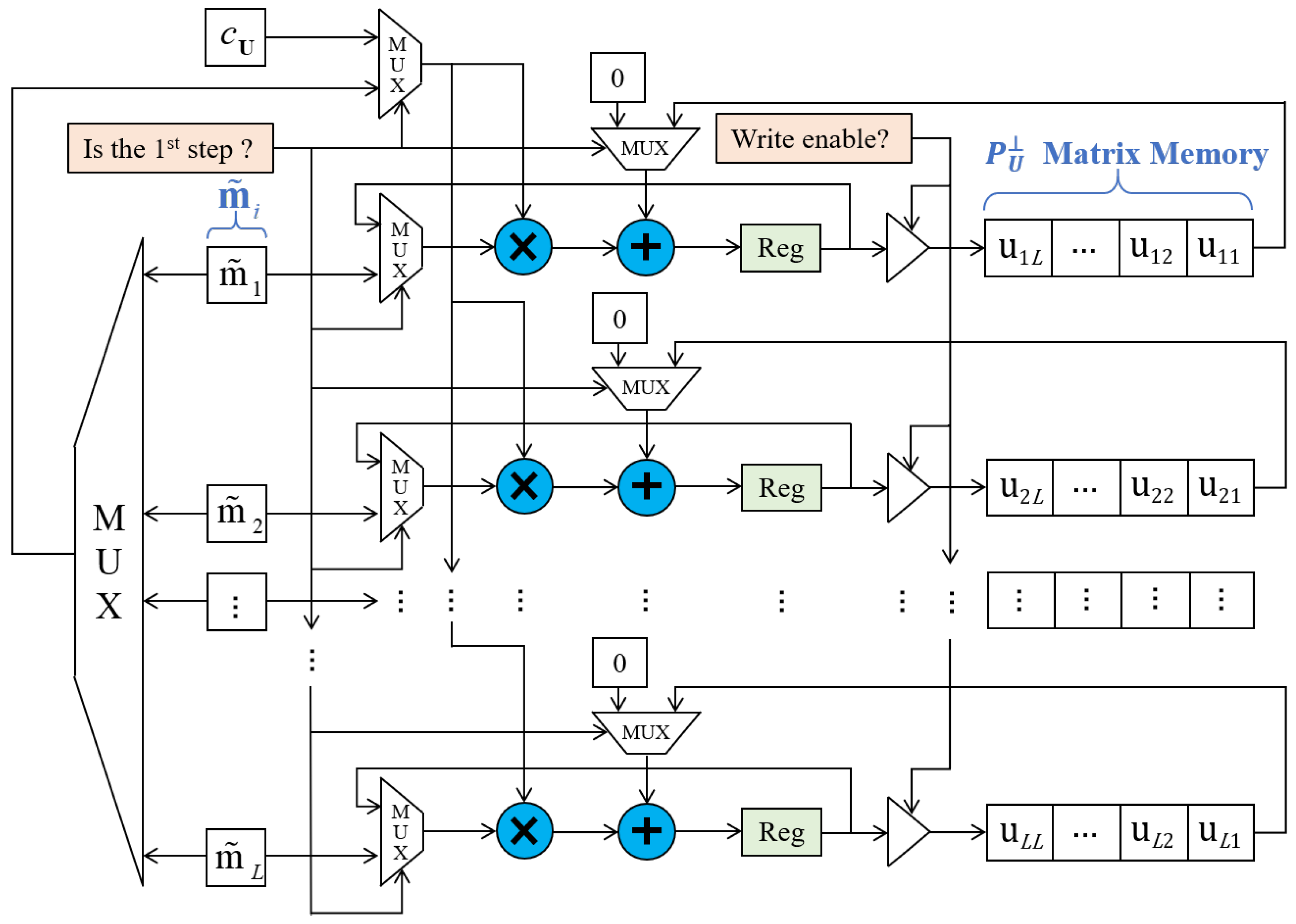
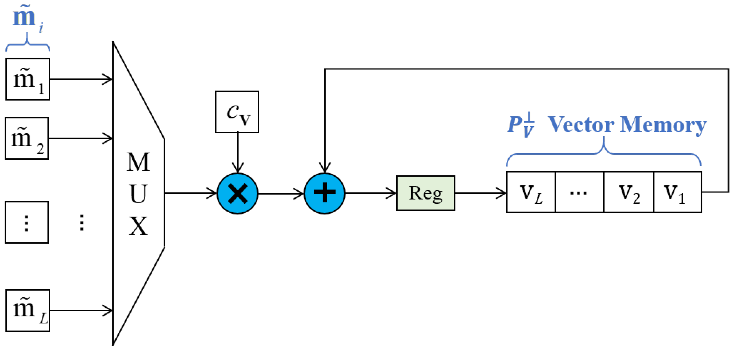
4.2.3. Updater
- (1)
- The data type of input data is 16 bits unsigned fixed-point (15 bits fractional part), while the majority of data types of intermediate data are not easy to assign. To better balance the trade-off between detection accuracy and resource consumption, different data types are used in different intermediate data. For example, as shown in Figure 2, the variable and are respectively set to 38 bits signed fixed-point type (10 bits integer part, 18 bits fractional part) and 36 bits signed fixed-point type (5 bits integer part, 31 bits fractional part). The elements of are 36 bits signed fixed-point type (10 bits integer part, 26 bits fractional part). All the other intermediate data are also assigned to the appropriate data type.
- (2)
- The elements of and are continuously updated and become smaller, so more bits should be assigned to the fractional part for avoiding data overflow. However, the fixed bit-width of and are recommended to be applied in order to reduce the resource consumption as much as possible. Considering the circumstances, we have done a lot of tests in HSIs and found that the variation trend of elements in was approximate to the inverse proportion function, so the values of elements were enlarged in a certain proportion in our implementation to ensure the variation trend constrained to a fixed interval. In this way, the risk of data overflow could be effectively avoided.
5. Experimental Results and Discussion
5.1. Experimental Environment
5.2. Hyperspectral Image Data Set
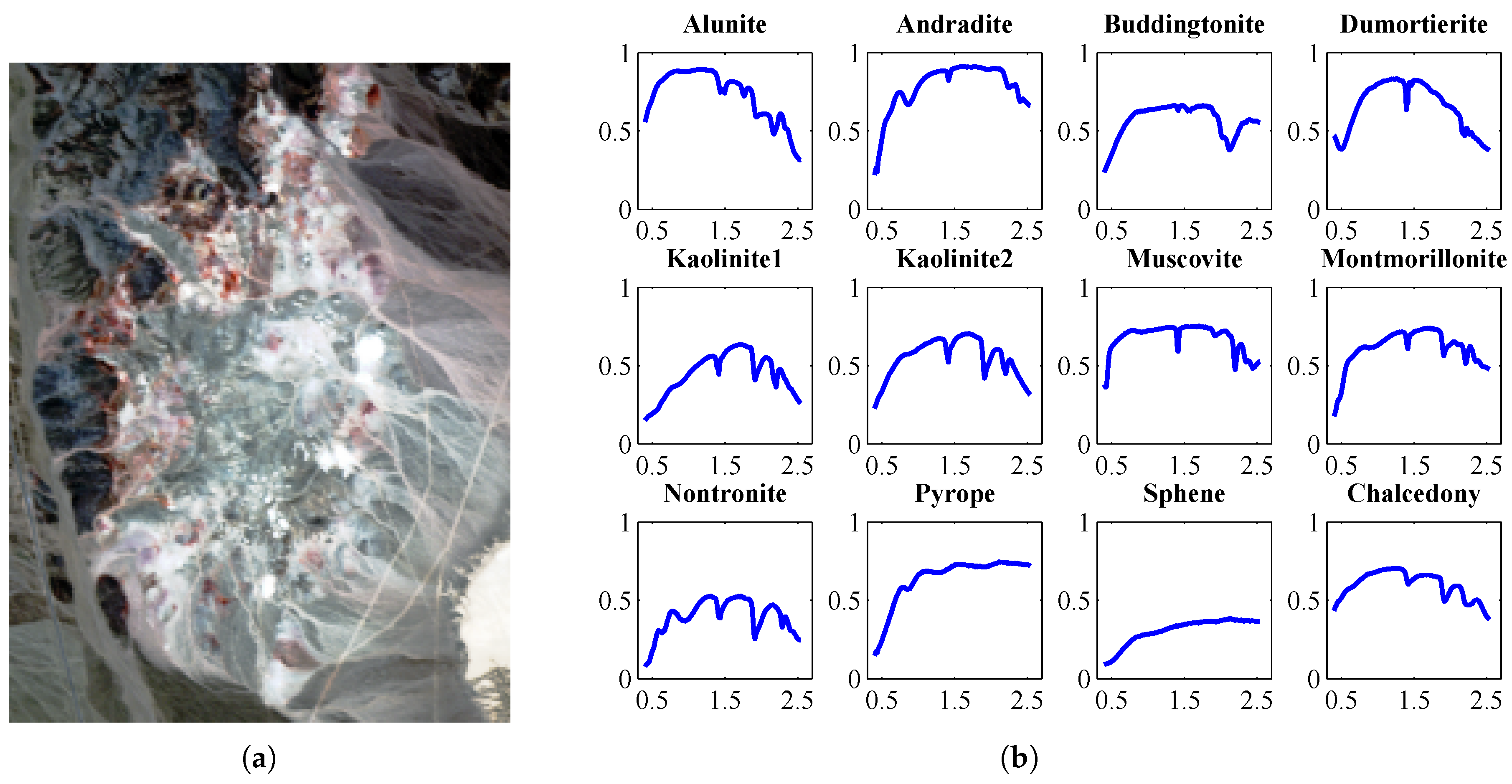
5.2.1. Cuprite Data
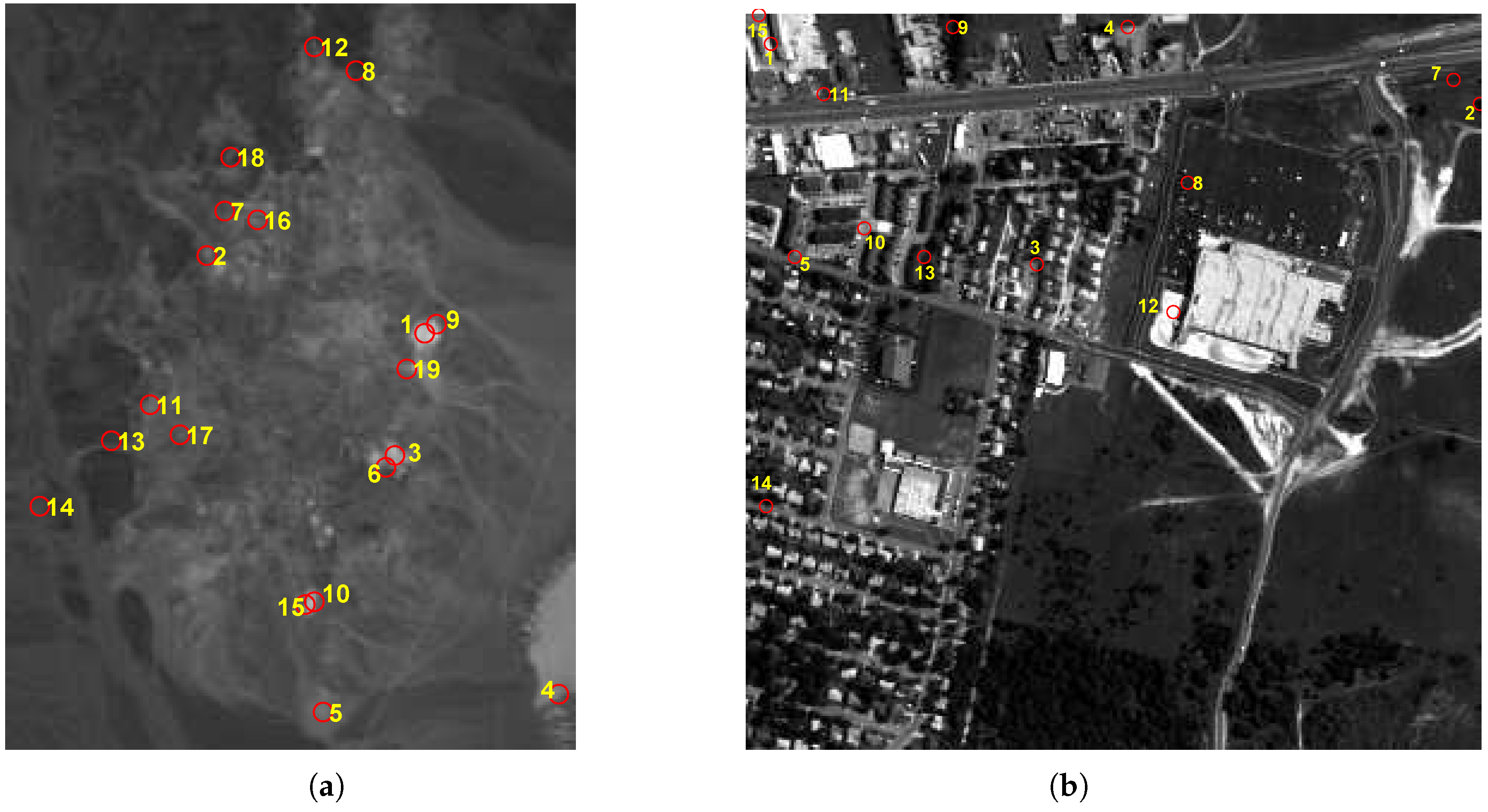
5.2.2. Urban Data
5.3. Analysis of Target Detection Accuracy
5.3.1. Results for the AVIRIS Cuprite Scene
5.3.2. Results with the HYDICE Urban Scene
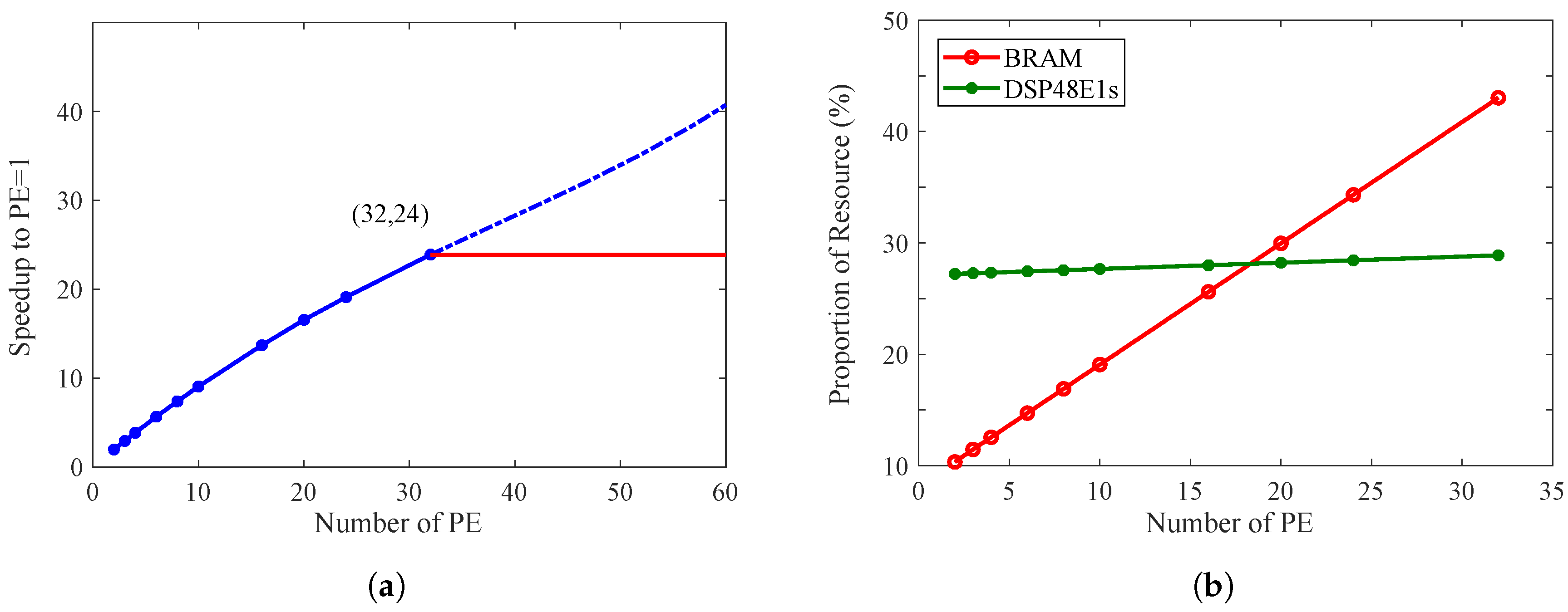
5.4. Performance Evaluation
5.5. Design Space Exploration and Potential Analysis
6. Conclusions
Author Contributions
Acknowledgments
Conflicts of Interest
Abbreviations
| HSI | Hyperspectral imagery |
| FPGA | Field programmable gate array |
| ATGP | Automatic target generation process |
| HLS | High-level synthesis |
| PE | Processing element |
References
- Manolakis, D.; Truslow, E.; Pieper, M.; Cooley, T.; Brueggeman, M. Detection algorithms in hyperspectral imaging systems: An overview of practical algorithms. IEEE Signal Process. Mag. 2014, 31, 24–33. [Google Scholar] [CrossRef]
- Ghamisi, P.; Yokoya, N.; Li, J. Advances in hyperspectral image and signal processing: A comprehensive overview of the state of the art. IEEE Geosci. Remote Sens. Mag. 2017, 5, 37–78. [Google Scholar] [CrossRef]
- Xie, W.; Shi, Y.; Li, Y.; Jia, X.; Lei, J. High-quality spectral-spatial reconstruction using saliency detection and deep feature enhancement. Pattern Recognit. 2019, 88, 139–152. [Google Scholar] [CrossRef]
- Sun, W.; Yang, G.; Du, B.; Zhang, L.; Zhang, L. A sparse and low-rank near-isometric linear embedding method for feature extraction in hyperspectral imagery classification. IEEE Trans. Geosci. Remote Sens. 2017, 55, 4032–4046. [Google Scholar] [CrossRef]
- Li, Y.; Xie, W.; Li, H. Hyperspectral image reconstruction by deep convolutional neural network for classification. Pattern Recognit. 2017, 63, 371–383. [Google Scholar] [CrossRef]
- Zhao, W.; Du, S. Spectral–spatial feature extraction for hyperspectral image classification: A dimension reduction and deep learning approach. IEEE Trans. Geosci. Remote Sens. 2016, 54, 4544–4554. [Google Scholar] [CrossRef]
- Sun, W.; Tian, L.; Xu, Y.; Du, B.; Du, Q. A randomized subspace learning based anomaly detector for hyperspectral imagery. Remote Sens. 2018, 10, 417. [Google Scholar] [CrossRef]
- Nasrabadi, N.M. Hyperspectral target detection: An overview of current and future challenges. IEEE Signal Process. Mag. 2014, 31, 34–44. [Google Scholar] [CrossRef]
- Chen, Y.; Lin, Z.; Zhao, X.; Wang, G.; Gu, Y. Deep learning-based classification of hyperspectral data. IEEE J. Sel. Top. Appl. Earth Obs. Remote Sens. 2014, 7, 2094–2107. [Google Scholar] [CrossRef]
- Sun, W.; Ma, J.; Yang, G.; Du, B.; Zhang, L. A Poisson nonnegative matrix factorization method with parameter subspace clustering constraint for endmember extraction in hyperspectral imagery. ISPRS J. Photogramm. Remote Sens. 2017, 128, 27–39. [Google Scholar] [CrossRef]
- Chen, S.Y.; Ouyang, Y.C.; Lin, C.; Chen, H.M.; Gao, C.; Chang, C.-I. Progressive endmember finding by fully constrained least squares method. In Proceedings of the Workshop on Hyperspectral Image and Signal Processing: Evolution in Remote Sensing (WHISPERS), Tokyo, Japan, 2–5 June 2015; pp. 1–4. [Google Scholar]
- Ren, H.; Chang, C.-I. Automatic spectral target recognition in hyperspectral imagery. IEEE Trans. Aerosp. Electron. Syst. 2003, 39, 1232–1249. [Google Scholar]
- Zhao, L.; Lin, W.; Wang, Y.; Li, X. Recursive local summation of rx detection for hyperspectral image using sliding windows. Remote Sens. 2018, 10, 103. [Google Scholar] [CrossRef]
- Yu, C.; Lee, L.C.; Chang, C.-I.; Xue, B.; Song, M.; Chen, J. Band-Specified Virtual Dimensionality for Band Selection: An Orthogonal Subspace Projection Approach. IEEE Trans. Geosci. Remote Sens. 2018, 56, 2822–2832. [Google Scholar] [CrossRef]
- Chang, C.-I.; Chen, S.Y.; Li, H.C.; Chen, H.M.; Wen, C.H. Comparative study and analysis among ATGP, VCA, and SGA for finding endmembers in hyperspectral imagery. IEEE J. Sel. Top. Appl. Earth Obs. Remote Sens. 2016, 9, 4280–4306. [Google Scholar] [CrossRef]
- Chang, C.-I.; Li, Y. Recursive band processing of automatic target generation process for finding unsupervised targets in hyperspectral imagery. IEEE Trans. Geosci. Remote Sens. 2016, 54, 5081–5094. [Google Scholar] [CrossRef]
- Gonzalez, C.; Bernabe, S.; Mozos, D.; Plaza, A. FPGA implementation of an algorithm for automatically detecting targets in remotely sensed hyperspectral images. IEEE J. Sel. Top. Appl. Earth Obs. Remote Sens. 2016, 9, 4334–4343. [Google Scholar] [CrossRef]
- Bernabe, S.; Lopez, S.; Plaza, A.; Sarmiento, R. GPU implementation of an automatic target detection and classification algorithm for hyperspectral image analysis. IEEE Geosci. Remote Sens. Lett. 2013, 10, 221–225. [Google Scholar] [CrossRef]
- Chang, C.-I.; Gao, C.; Chen, S.Y. Recursive Automatic Target Generation Process in Subpixel Detection. IEEE Geosci. Remote Sens. Lett. 2015, 12, 1848–1852. [Google Scholar] [CrossRef]
- Plaza, A.J. Special issue on architectures and techniques for real-time processing of remotely sensed images. J. Real Time Image Process. 2009, 4, 191–193. [Google Scholar] [CrossRef]
- Li, X.; Huang, B.; Zhao, K. Massively parallel GPU design of automatic target generation process in hyperspectral imagery. IEEE J. Sel. Top. Appl. Earth Obs. Remote Sens. 2015, 8, 2862–2869. [Google Scholar] [CrossRef]
- Gonzalez, C.; Lopez, S.; Mozos, D.; Sarmiento, R. A novel FPGA-based architecture for the estimation of the virtual dimensionality in remotely sensed hyperspectral images. J. Real Time Image Process. 2018, 15, 297–308. [Google Scholar] [CrossRef]
- Chang, C.-I.; Li, Y.; Wang, Y. Progressive Band Processing of Fast Iterative Pixel Purity Index for Finding Endmembers. IEEE Geosci. Remote Sens. Lett. 2017, 14, 1464–1468. [Google Scholar] [CrossRef]
- Yang, B.; Yang, M.; Plaza, A.; Gao, L.; Zhang, B. Dual-mode FPGA implementation of target and anomaly detection algorithms for real-time hyperspectral imaging. IEEE J. Sel. Top. Appl. Earth Obs. Remote Sens. 2015, 8, 2950–2961. [Google Scholar] [CrossRef]
- Vellas, S.; Lentaris, G.; Maragos, K.; Soudris, D.; Kandylakis, Z.; Karantzalos, K. FPGA acceleration of hyperspectral image processing for high-speed detection applications. In Proceedings of the IEEE International Symposium on Circuits and Systems (ISCAS), Baltimore, MD, USA, 28–31 May 2017; pp. 1–4. [Google Scholar]
- Pei, S.; Wang, R.; Zhang, J.; Jin, Y. FPGA-based Acceleration for Hyperspectral Image Analysis. In Proceedings of the IEEE Advanced Information Technology, Electronic and Automation Control Conference (IAEAC), Chongqing, China, 24–26 March 2017; pp. 324–327. [Google Scholar]
- Nane, R.; Sima, V.M.; Pilato, C.; Choi, J.; Fort, B.; Canis, A.; Anderson, J. A survey and evaluation of FPGA high-level synthesis tools. IEEE Trans. Comput.-Aided Des. Integr. Circuits Syst. 2016, 35, 1591–1604. [Google Scholar] [CrossRef]
- Cong, J.; Liu, B.; Neuendorffer, S.; Noguera, J.; Vissers, K.; Zhang, Z. High-level synthesis for FPGAs: From prototyping to deployment. IEEE Trans. Comput.-Aided Des. Integr. Circuits Syst. 2011, 30, 473–491. [Google Scholar] [CrossRef]
- Domingo, R.; Salvador, R.; Fabelo, H.; Madronal, D.; Ortega, S.; Lazcano, R. High-level design using Intel FPGA OpenCL: A hyperspectral imaging spatial-spectral classifier. In Proceedings of the International Symposium on Reconfigurable Communication-centric Systems-on-Chip (ReCoSoC), Madrid, Spain, 12–14 July 2017; pp. 1–8. [Google Scholar]
- Desai, P.; Aslan, S.; Saniie, J. FPGA Implementation of Gram-Schmidt QR Decomposition Using High Level Synthesis. In Proceedings of the IEEE International Conference on Electro Information Technology (EIT), Lincoln, NE, USA, 14–17 May 2017; pp. 482–487. [Google Scholar]
- Ma, S.; Shi, X.; Andrews, D. Parallelizing maximum likelihood classification (MLC) for supervised image classification by pipelined thread approach through high-level synthesis (HLS) on FPGA cluster. Big Earth Data 2018, 1–15. [Google Scholar] [CrossRef]
- Guerra, R.; López, S.; Sarmiento, R. A FPGA implementation for linearly unmixing a hyperspectral image using OpenCL. In High-Performance Computing in Geoscience and Remote Sensing VII; International Society for Optics and Photonics: Bellingham, WA, USA, 2017; p. 104300D. [Google Scholar]
- Santos, L.; Berrojo, L.; Moreno, J.; Lopez, J.F.; Sarmiento, R. Multispectral and hyperspectral lossless compressor for space applications (HyLoC): A low-complexity FPGA implementation of the CCSDS 123 standard. IEEE J. Sel. Top. Appl. Earth Obs. Remote Sens. 2016, 9, 757–770. [Google Scholar] [CrossRef]
- Lei, J.; Li, Y.; Zhao, D.; Xie, J.; Chang, C.I.; Wu, L. A Deep Pipelined Implementation of Hyperspectral Target Detection Algorithm on FPGA Using HLS. Remote Sens. 2018, 10, 516. [Google Scholar] [CrossRef]
- Guo, J.; Li, Y.; Liu, K.; Lei, J.; Wang, K. Fast FPGA Implementation for Computing the Pixel Purity Index of Hyperspectral Images. J. Circuits Syst. Comput. 2018, 27, 1850045. [Google Scholar] [CrossRef]
- Chang, C.-I.; Wu, C.C.; Tsai, C.T. Random N-finder (N-FINDR) endmember extraction algorithms for hyperspectral imagery. IEEE Trans. Image Process. 2011, 2011, 641–656. [Google Scholar] [CrossRef] [PubMed]
- Gao, C.; Chang, C.-I. Recursive automatic target generation process for unsupervised hyperspectral target detection. In Proceedings of the IEEE International Geoscience and Remote Sensing Symposium (IGARSS), Quebec, QC, Canada, 13–18 July 2014; pp. 3598–3601. [Google Scholar]
- Song, M.; Li, H.C.; Chang, C.-I.; Li, Y. Gram-Schmidt orthogonal vector projection for hyperspectral unmixing. In Proceedings of the IEEE International Geoscience and Remote Sensing Symposium (IGARSS), Quebec, QC, Canada, 13–18 July 2014; pp. 2934–2937. [Google Scholar]
- Geng, X.; Yang, W.; Ji, L.; Ling, C.; Yang, S. A Piecewise Linear Strategy of Target Detection for Multispectral/Hyperspectral Image. IEEE J. Sel. Top. Appl. Earth Obs. Remote Sens. 2018, 11, 951–961. [Google Scholar] [CrossRef]
- Xu, F.; Lv, Y.; Xu, X.; Dinavahi, V. FPGA-Based real-time wrench model of direct current driven magnetic levitation actuator. IEEE Trans. Ind. Electron. 2018. [Google Scholar] [CrossRef]
- Hahne, C.; Lumsdaine, A.; Aggoun, A.; Velisavljevic, V. Real-time refocusing using an FPGA-based standard plenoptic camera. IEEE Trans. Ind. Electron. 2018. [Google Scholar] [CrossRef]
- Zhang, H.; Li, Y.; Zhang, Y.; Shen, Q. Spectral-spatial classification of hyperspectral imagery using a dual-channel convolutional neural network. Remote Sens. Lett. 2017, 8, 438–447. [Google Scholar] [CrossRef] [Green Version]
- Guerra, R.; Martel, E.; Khan, J.; Lopez, S.; Athanas, P.; Sarmiento, R. On the Evaluation of Different High-Performance Computing Platforms for Hyperspectral Imaging: An OpenCL-Based Approach. IEEE J. Sel. Top. Appl. Earth Obs. Remote Sens. 2017, 10, 4879–4897. [Google Scholar] [CrossRef]
- Zhu, F.; Wang, Y.; Xiang, S.; Fan, B.; Pan, C. Structured sparse method for hyperspectral unmixing. ISPRS J. Photogramm. Remote Sens. 2014, 88, 101–118. [Google Scholar] [CrossRef]
- Guo, Q.; Pu, R.; Gao, L.; Zhang, B. A novel anomaly detection method incorporating target information derived from hyperspectral imagery. Remote Sens. Lett. 2016, 7, 11–20. [Google Scholar] [CrossRef]
- Roussel, G.; Weber, C.; Briottet, X.; Ceamanos, X. Comparison of two atmospheric correction methods for the classification of spaceborne urban hyperspectral data depending on the spatial resolution. Int. J. Remote Sens. 2018, 39, 1593–1614. [Google Scholar] [CrossRef]
- Panda, A.; Pradhan, D. Hyperspectral image processing for target detection using Spectral Angle Mapping. In Proceedings of the IEEE International Conference on Industrial Instrumentation and Control (ICIC), Pune, India, 28–30 May 2015; pp. 1098–1103. [Google Scholar]
- Dumke, I.; Nornes, S.M.; Purser, A.; Marcon, Y.; Ludvigsen, M.; Ellefmo, S.L. First hyperspectral imaging survey of the deep seafloor: High-resolution mapping of manganese nodules. Remote Sens. Environ. 2018, 209, 19–30. [Google Scholar] [CrossRef]
- Chang, C.-I. A review of virtual dimensionality for hyperspectral imagery. IEEE J. Sel. Top. Appl. Earth Obs. Remote Sens. 2018. [Google Scholar] [CrossRef]


| Stage Number | Formula | Flop |
|---|---|---|
| 1 | ||
| 2 | ||
| 3 |
| Stage Number | Formula | Flop |
|---|---|---|
| 1 | ||
| 2 | ||
| 3 | r |
| ATGP-OSP | Fast-ATGP | |
|---|---|---|
| Alunite | ||
| Andradite | ||
| Buddingtonite | ||
| Dumortierite | ||
| Kaolinite | ||
| Kaolinite | ||
| Muscovite | ||
| Montmorillonite | ||
| Nontronite | ||
| Pyrope | ||
| Sphene | ||
| Chalcedony | ||
| Average |
| Version | Asphalt Road | Tree | Roof | Dirt | Average |
|---|---|---|---|---|---|
| ATGP-OSP | |||||
| Fast-ATGP |
| HSIs | C++ (s) | FPGA (s) |
|---|---|---|
| Cuprite | 210.016 | 0.0376 |
| Urban | 320.636 | 0.0491 |
| ATGP-OSP | Fast-ATGP | |
|---|---|---|
| Maximum frequency (MHz) | 72 | 200 |
| Number of clock periods | ||
| Total time (s) | 1.29 | 0.0376 |
| Speedup | 34.3× | |
| ATGP-OSP | Fast-ATGP | |||
|---|---|---|---|---|
| Number | Proportion | Number | Proportion | |
| BRAMs | 994 | 67.62% | 632.5 | 43.03% |
| DSP48E1s | 2847 | 79.08% | 1040 | 28.89% |
| Slice LUTs | 132,802 | 30.66% | 80,080 | 18.49% |
| Slice Registers | 22,962 | 2.65% | 14,0143 | 16.18% |
© 2019 by the authors. Licensee MDPI, Basel, Switzerland. This article is an open access article distributed under the terms and conditions of the Creative Commons Attribution (CC BY) license (http://creativecommons.org/licenses/by/4.0/).
Share and Cite
Lei, J.; Wu, L.; Li, Y.; Xie, W.; Chang, C.-I.; Zhang, J.; Huang, B. A Novel FPGA-Based Architecture for Fast Automatic Target Detection in Hyperspectral Images. Remote Sens. 2019, 11, 146. https://0-doi-org.brum.beds.ac.uk/10.3390/rs11020146
Lei J, Wu L, Li Y, Xie W, Chang C-I, Zhang J, Huang B. A Novel FPGA-Based Architecture for Fast Automatic Target Detection in Hyperspectral Images. Remote Sensing. 2019; 11(2):146. https://0-doi-org.brum.beds.ac.uk/10.3390/rs11020146
Chicago/Turabian StyleLei, Jie, Lingyun Wu, Yunsong Li, Weiying Xie, Chein-I Chang, Jintao Zhang, and Biying Huang. 2019. "A Novel FPGA-Based Architecture for Fast Automatic Target Detection in Hyperspectral Images" Remote Sensing 11, no. 2: 146. https://0-doi-org.brum.beds.ac.uk/10.3390/rs11020146