An Adaptive End-to-End Classification Approach for Mobile Laser Scanning Point Clouds Based on Knowledge in Urban Scenes

Abstract

It is fundamental for 3D city maps to efficiently classify objects of point clouds in urban scenes. However, it is still a large challenge to obtain massive training samples for point clouds and to sustain the huge training burden. To overcome it, a knowledge-based approach is proposed. The knowledge-based approach can explore discriminating features of objects based on people’s understanding of the surrounding environment, which exactly replaces the role of training samples. To implement the approach, a two-step segmentation procedure is carried out in this paper. In particular, Fourier Fitting is applied for second adaptive segmentation to separate points of multiple objects lying within a single group of the first segmentation. Then height difference and three geometrical eigen-features are extracted. In comparison to common classification methods, which need massive training samples, only basic knowledge of objects in urban scenes is needed to build an end-to-end match between objects and extracted features in the proposed approach. In addition, the proposed approach has high computational efficiency because of no heavy training process. Qualitative and quantificational experimental results show the proposed approach has promising performance for object classification in various urban scenes.

1. Introduction

Point clouds collected by mobile LiDAR systems are frequently used for various 3D city mapping applications, such as urban planning, city infrastructure construction, and intelligent transportation systems, etc. Taking intelligent transportation systems as an example, updated city maps that include the location of urban objects and traffic signs are useful for navigation, which could be used to decrease traffic congestion, lessen the risk of accidents, and develop self-driving systems [1,2].

3D city maps could be created and updated from various perspectives by mapping objects. Many elements, including user requirements, map contents, accuracy, scale, and so on, all are very important in 3D mapping. Before an object can be mapped, it needs to be classified in point clouds. Many approaches in recent publications already acquired excellent results for point cloud classification for this line of research [3,4,5,6,7,8,9,10,11]. However, these approaches still have three main challenges.

(1) These approaches all strongly belong to the category of supervised learning. Lots of training samples are required to learn discriminating features of different classes. However, most available benchmarks of point clouds are manually labeled, which is labor-intensive and time-consuming.

(2) In these publications, training and test samples are strongly correlative with several “sameness”. For example, researchers normally divide a complete dataset into several files, with half for training and the other half for testing. These files should share some “sameness”, such as sensor, period, and area of data acquisition. The robustness for these methods is challenged when applied in other scenes.

(3) Due to necessary training process, most of above approaches achieve performance at the cost of the heavy computation burden.

To overcome these problems, the following solutions provide good inspiration.

(1) Knowledge-based approaches can be employed, which explore discriminating features of objects based on people’s understanding of the surrounding environment. Therefore, massive training samples are not needed. Already in the early 90s, knowledge-based system had been proposed for image and point cloud processing [12,13,14,15]. Recently, the line of research has been active again [16].

(2) To enhance the robustness of methods, it is critical to exploit discriminating characteristics of urban objects which are not easily affected by the external environment. Geometric features, which are reflected by several closely spaced points, have always been considered for discriminating feature extraction. Furthermore, knowledge-based approaches can help to realize the extraction of geometric features.

(3) The knowledge-based approach can save lots of computation time with no heavy training process.

Based on the above inspirations, the knowledge-based approach is investigated in three parts, i.e., close spaces of points, the defining of geometric features, and knowledge-based object classification.

Firstly, segmentation is a common way of grouping the point clouds into spaced neighborhood [3,17,18,19,20,21,22,23,24]. A Link-Chain method based on a super-voxel segmentation of sparse 3D data obtained from LiDAR sensors was presented to segment and classify 3D urban point clouds [3]. Vosselman et al. [18] performed a voxelization to divide the point cloud space in a 3D grid of small regular cubes whose resolution depends on the size of the grid cells. Yang et al. [21] generated multi-scale supervoxels from scattered mobile laser scanning points to improve the estimation of local geometric structures of neighboring points. Alexander et al. [24] described a connected component segmentation approach for segmenting organized point cloud data. In this paper, a two-step segmentation procedure is performed. In the first step, a cubic bounding box based on x, y, and z coordinates of points is set up and then segmented into lots of small cubes. Based on the results of the first segmentation, Fourier Fitting (FF) for second adaptive segmentation is applied. As there are points of multiple object classes lying within a single block of the first segmentation, FF can adaptively separate these points into several groups. FF had been used in some point cloud and satellite data research [25,26]. The outputs of the two-step segmentation are respectively called the 3D block and the 3D sub-block.

Secondly, available geometric features from many closely spaced points need to be extracted. Some approaches had been known in the literature for feature extraction of laser scanner point clouds [5,27,28,29]. Pouria et al. [5] extracted seven main features (geometrical shape, height above ground, and planarity, etc.) to train their classifier for object recognition, including cars, bicycles, buildings, pedestrians, and street signs, in 3D point clouds of urban street scene. Wang et al. [27] listed the geometric features and additional statistical features to classify Ground, Building, and Vegetation. Li et al. [28] proposed a knowledge-based approach that uses geometric features including size, shape, height. The study of three eigenvalues obtained from the covariance matrix of each segment was developed to detect geometrical shapes of urban objects [29]. Chehata et al. [30] defined height difference between the LiDAR point and the lowest point found in a large cylindrical volume. The feature helped discriminate ground and off-ground object in his work. In the paper, the height information and geometrical eigen-features are defined as an initial set of features from which to begin the research.

Finally, made-up labels for geometrical features are created to classify objects. For instance, height difference of points in blocks, $\Delta h$, is represented by made-up label $L_i$, $i\in \{1,2,3\}$. $L_i$ has three probable levels, (i) $L_1=0:\Delta h<H{D}_1$, (ii) $L_2=1:H{D}_1\le \Delta h<H{D}_2$, (iii) $L_3=2:\Delta h\ge H{D}_2$. Here $H{D}_1$ and $H{D}_2$ are two experiential thresholds of height difference. Every sub-block is presented by a vector expression of the combination of made-up labels. Based on people’s understanding of surrounding environment, each combination finally points directly to an object class. An end-to-end match between combinations of made-up labels and object classes is therefore built.

In summary, the paper presents an adaptive end-to-end classification approach for mobile laser scanning point clouds based on the knowledge in urban scenes. This paper includes the experiments in a point cloud benchmark, which quantificationally demonstrate the feasibility of the knowledge-based approach for classifying objects. The approach is also qualitatively tested in another urban scene to demonstrate its robustness. The main contribution of the work in the paper include:

(1) A knowledge-based approach to extract discriminating geometrical features is proposed. The motivation is to overcome the requirement of massive training samples, also to avoid the time-consuming training process;

(2) FF for second segmentation is introduced. In most cases, there are points of multiple object classes lying within a single block of the first segmentation. Fourier Fitting can adaptively divide these points into several sub-blocks;

(3) An end-to-end match is built between actual object classes and the combinations of made-up labels. It can intentionally highlight discriminating characteristics for each object class and realize quick object classification.

The remainder of this paper is organized as follows. Section 2 introduces the proposed approach. Section 3 discusses the experiment and result analysis, and Section 4 presents the conclusion and future work.

2. Methodology

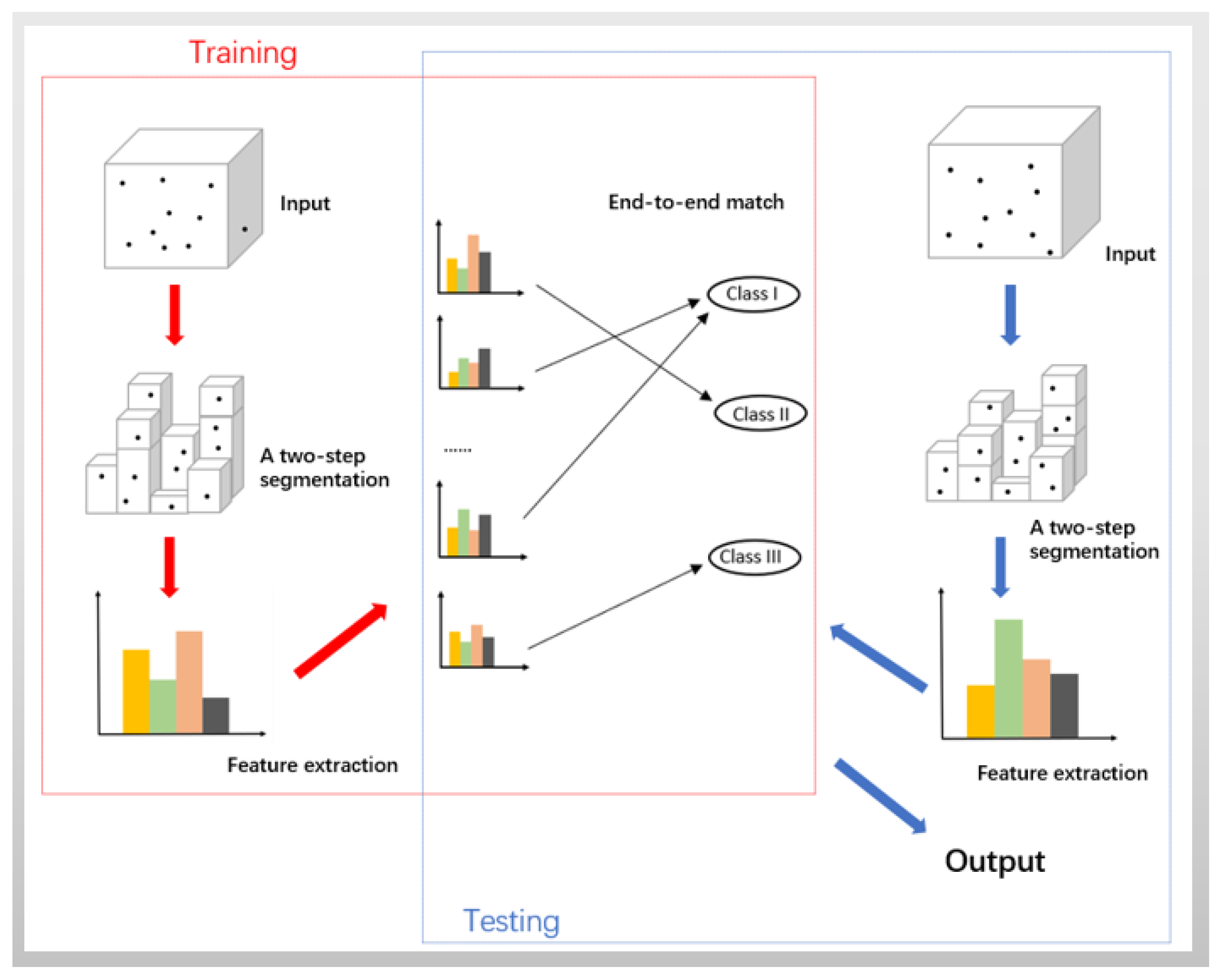
The propose of this paper is to exploit discriminating features of urban objects which are not easily affected by the external environment, and to build an end-to-end match between the combinations of made-up labels and object classes. In the section, four parts including class defining, segmentation, feature exploring, and the rule of end-to-end match, are discussed to complete a whole procedure. Figure 1 gives the proposed workflow.

2.1. Class Defining

The type of object class, which greatly determines the methods of segmentation and the types of extracted features, should be initially defined. The datasets selected in the paper include one mobile laser scanning benchmark covering the main street in Paris, France [31], and another one from a company Cyclomedia, which mainly covers city scenes in Schiedam, Netherlands. Considering the variety of objects in these two datasets, three classes (i.e., Facade, Ground and Others) are defined in the paper.

2.2. Segmentation

A two-step segmentation procedure is carried out in the paper. The complete point cloud will be firstly segmented into 3D blocks and further into 3D sub-blocks secondly. A block normally consists of one or several sub-blocks. There is no intersection of points among 3D blocks and among 3D sub-blocks.

2.2.1. First Segmentation

Logically, objects own their individual locations on the plane of x and y coordinates, except the special case that the projected areas of several objects overlap on the plane, for instance, a tree and the bike under it. At the first segmentation, a cubic division is applied.

The point cloud is divided into 3D blocks through the following process. Given the point cloud dataset, the maximum and minimum of x, y coordinates on the 2D plane is figured out, i.e., $x_{min}$, $x_{max}$, $y_{min}$, $y_{max}$. Then a plane bounding rectangle of the whole point cloud is set up, i.e., [$x_{min}$, $y_{min}$] × [$x_{max}$, $y_{max}$]. The rectangle is divided into a $M\times N$ grid of tiles, whose length and width of each tile are both R. $N_y$ is the smallest integer larger than ($y_{max}$ − $y_{min}$)/R, $N_x$ is the smallest integer larger than ($x_{max}$ − $x_{min}$)/R. Adding the z coordinate for each point in each tile, the 2D tile could be extended to a 3D block, of which the height is decided by the distance of the highest and lowest points inside the 3D block.

2.2.2. Second Segmentation

In some cases, there are points of multiple object classes lying within a single 3D block of the first segmentation. Therefore, spatial distribution of points per 3D block is explored during the second segmentation.

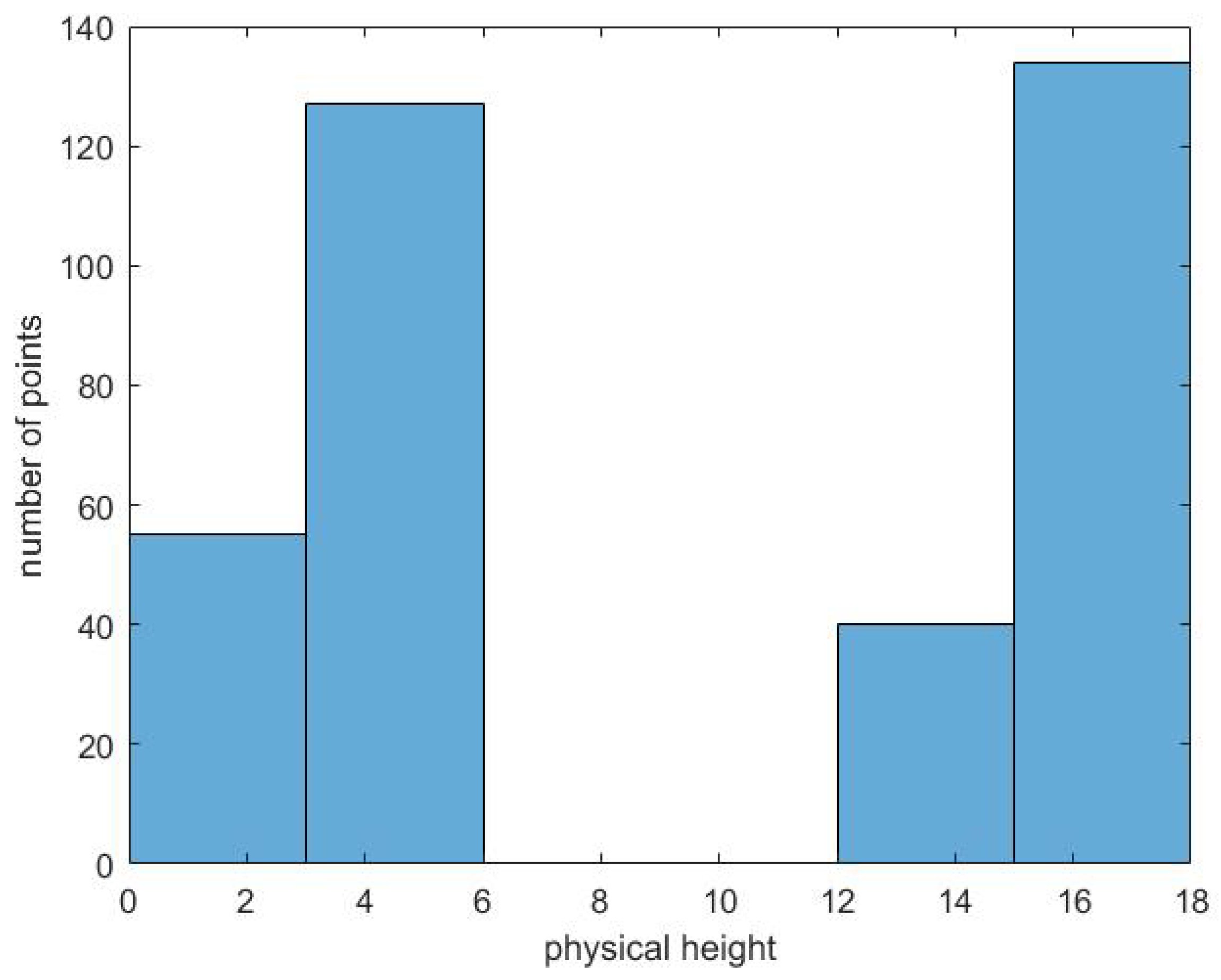
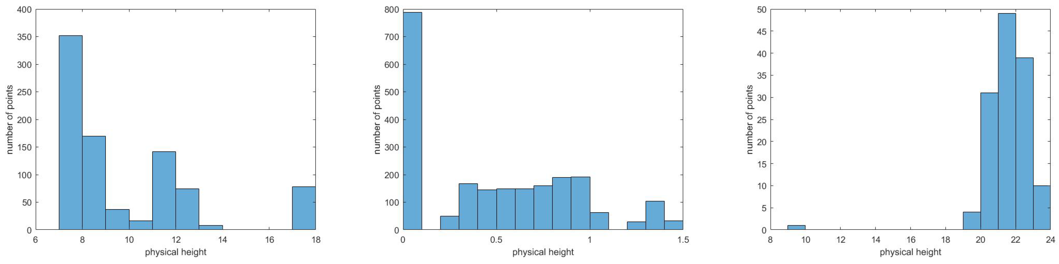
The simplest way is to vertically slice a 3D block into several sub-blocks with a fixed interval. In Figure 2, the variable on the horizontal axis is z coordinate of points, called physical height h (m), and the variable on the vertical axis is the number of points. Figure 2 shows that points separately locate in two ranges on the horizontal axis. There is no point in the middle range. Equal slice with a fixed interval (e.g., 2.5 m) forcedly separates these clustered points resulting probably in breaking their integrality, and resulting in empty sub-blocks to occupy memory and computation time. Figure 3 also shows similar examples.

Instead of the segmentation with a fixed interval, FF is used. In early 1800s, the French mathematician Fourier [32] proposed that “any function can be represented by an infinite sum of sine and cosine terms.” The relationship between the physical height and the number of points can be fitted to a periodic function. The troughs of the fitting wave are boundaries, where points of multiple object classes within a single 3D block are adaptively separated into several 3D sub-blocks. The formula for FF is as follows:

$$y=a_0+a_{1}cos(w\ast x)+b_{1}sin(w\ast x)$$

(1)

especially,

$$\begin{array}{ccc}\hfill y& =& a_0+a_{1}cos(w\ast x)+b_{1}sin(w\ast x)\hfill \\ & =& a_0+\sqrt{a_1^2+b_1^2}sin(w\ast x+arctan\frac{a_1}{b_1})\hfill \end{array}$$

when

$$x=\frac{-\frac{\pi }{2}+2\ast k\ast \pi -arctan\frac{a_1}{b_1}}{w},k=0,1,2,\dots \dots$$

y gets the minimum value.

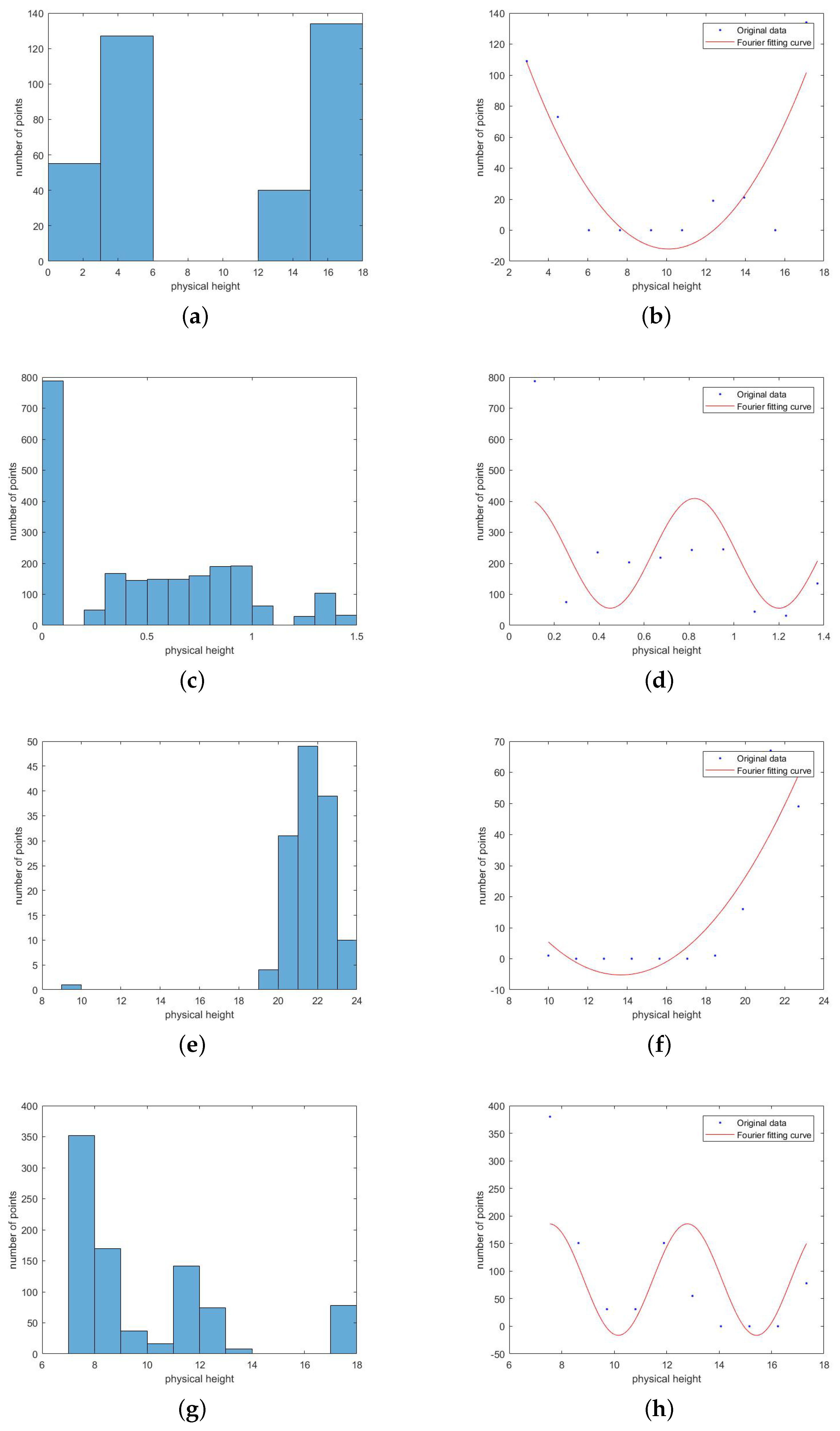
In Figure 4, several examples based on FF are visualized during the second segmentation. Figure 4a, for example, shows the histogram of the physical height of points and the number of points in a 3D block. There is one obvious gap on the horizontal axis. Correspondingly, there is exactly one wave trough in the fitting curve (Figure 4b). The discrete points (blue) are the numbers of points in every height interval. The waveform (red) is the fitting curve. The trough value 10 is the boundary threshold of the physical height to segment points into two sub-blocks.

2.3. Features Exploring

In the section, the focus is to explore height difference and geometrical eigen-features of objects.

2.3.1. Height Difference

Height difference, $\Delta h$, is used to filter ground points in the paper, as the terrain of both datasets selected is almost flat. $\Delta h$ is the distance of the z coordinate between the lowest and highest points of all points belonging to a 3D block. It is computed in each 3D block at the end of the first segmentation. The 3D blocks in grounds present a low height difference. However, vertical objects including facades and others, show a large height difference between their lowest and highest points. Two thresholds $H{D}_1$ and $H{D}_2$ of height difference are set. $H{D}_1$ is to filter ground points. $H{D}_2$ is to filter high objects, i.e., class Facade in the paper.

2.3.2. Geometrical Eigen-Features

Normally, the linearity feature can be used to detect line structures, the planarity feature can discriminate planar structures, and the scattering feature allows the exhibition of 3D structures [33,34]. At the end of the second segmentation, three geometrical eigen-features (e.g., linearity $L_{\lambda }$, planarity $P_{\lambda }$, and scattering $S_{\lambda }$) are defined to identify the shape of points in 3D sub-blocks. Details are given below.

Given a 3D point set $P_{set}=\{p_i=(x_i,y_i,z_i)|i=1,2,\dots ,n\}$ within a 3D block, an efficient method to compute and analyze the 3D point set $P_{set}$ is to diagonalize the covariance matrix of $P_{set}$. In a matrix form, the covariance matrix of $P_{set}$ is written as

$$C\left(P_{set}\right)=\frac{{\sum }_{p_i\in P_{set}}{w}_i{(p_i-\overline{p})}^T(p_i-\overline{p})}{{\sum }_i{w}_i}$$

where $\overline{p}$ represents the mean of the points, that is, $\overline{p}=\frac{1}{n}{\sum }_{i=1}^n{p}_i,$ and n represents the number of points in $P_{set}$. $w_i$ is the weight of point $p_i$, generally $w_i$ = 1. The eigenvectors and eigenvalues of the covariance matrix are computed by using a matrix diagonalization technique, that is, $V^{-1}CV=D$, where D is a diagonal matrix containing the eigenvalues, i.e., ${\lambda }_1,{\lambda }_2,{\lambda }_3$ of C. V is an orthogonal matrix that contains the corresponding eigenvectors. The obtained eigenvalues are greater than or equal to zero, that is, ${\lambda }_1\ge {\lambda }_2\ge {\lambda }_3\ge 0$. It is worth noting that the occurrence of eigenvalues identical to zero must be avoided by adding an infinitesimal small value. Situation ${\lambda }_1\gg {\lambda }_2,{\lambda }_3$ represents a stick-like ellipsoid, meaning a linear structure. Situation ${\lambda }_1\approx {\lambda }_2\gg {\lambda }_3$ indicates a flat ellipsoid, representing a planar structure. Situation ${\lambda }_1\approx {\lambda }_2\approx {\lambda }_3$ corresponds to a volumetric structure. Based on the geometrical property, three geometrical eigen-features are defined [35]. Here the definitions of the eigen-features of linearity $L_{\lambda }$, planarity $P_{\lambda }$, and sphericity $S_{\lambda }$ are given as follows:

$$L_{\lambda }=\frac{{\lambda }_1-{\lambda }_2}{{\lambda }_1}$$

$$P_{\lambda }=\frac{{\lambda }_2-{\lambda }_3}{{\lambda }_1}$$

$$S_{\lambda }=\frac{{\lambda }_3}{{\lambda }_1}$$

where $L_{\lambda }+P_{\lambda }+S_{\lambda }=1.$

2.4. The Rule of End-To-End Match

In Section 2.2, lots of 3D blocks are achieved at the first segmentation. These 3D blocks are further divided into the lots of 3D sub-blocks based on FF at the second segmentation. During the process of the two-step segmentation, height difference and geometrical eigen-features are extracted according to Section 2.3. In this section, made-up labels in terms of extracted features for classifying the objects are introduced. The base of made-up labeling is the knowledge, that is, people’s understanding of the extracted features. Simply speaking, every sub-block is given a made-up label based on height difference of points. Then we use the three eigen-features of points inside the sub-block to generate another label. As a result, the sub-block is presented by a 2D vector expression of the combination of these two made-up labels. The process includes the following two aspects in detail.

On the one hand, each 3D block is given a made-up label at the end of the first segmentation based on two thresholds of height difference $H{D}_1,H{D}_2$. For example, given a 3D block B and in which height difference of points is ${\Delta }_B$. The made-up label $L_B$ of the 3D block B at the first segmentation is marked as follows:

$$L_B=\left\{\begin{array}{cc}0,\hfill & \mathrm{if}{\Delta }_B<H{D}_1\hfill \\ 1,\hfill & \mathrm{if}H{D}_1\le {\Delta }_B<H{D}_2\hfill \\ 2,\hfill & \mathrm{if}{\Delta }_B\ge H{D}_2\hfill \end{array}\right.$$

(2)

On the other hand, given a sub-block b which is a subset of the 3D block B, three eigen-features of b separately are $L_{b,\lambda }$, $P_{b,\lambda }$, and $S_{b,\lambda }$. The shape of points in the sub-block b is identified based on two thresholds $l_{\lambda },p_{\lambda }$. The made-up label $L_b$ of the sub-block b at the second segmentation follows the rule: $L_b$ is set to be 0 if $P_{b,\lambda }>p_{\lambda }$, or set to be 1 for $L_{b,\lambda }>l_{\lambda }$, or 2 for other cases.

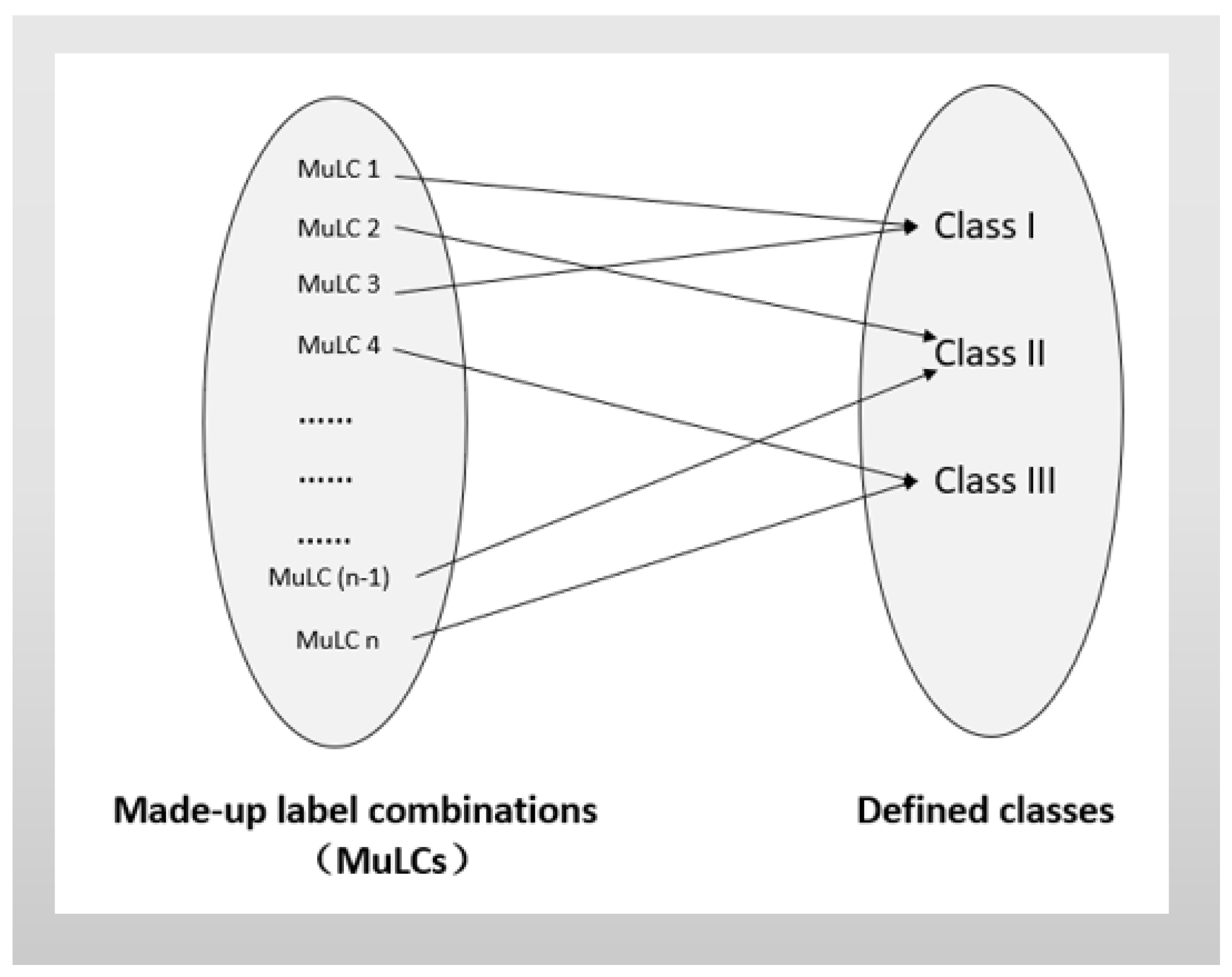
As b is a subset of B, the made-up label of b is as the same as B’s at the first segmentation. Therefore, combining these two made-up results, the sub-block b is manually marked as $[L_B,L_b]$, $L_B\in \{0,1,2\},L_b\in \{0,1,2\}.$ In total there are nine combinations of made-up labels. Without loss of generality, suppose that the combination of made-up labels of b is $[2,0]$, the first element “2” means the height difference $\Delta h$ of points of the block B is larger than $H{D}_2$ at the first segmentation. The second element “0” means the shape of clustered points of the sub-block b looks linear at the second segmentation. The idea to set rules of end-to-end match is simple. The three defined classes are counted, which each combination of made-up labels corresponds to for the training dataset. Then an optimal surjective relation from the combinations of made-up labels to the three classes are produced. The expected diagram is in Figure 5.

In the paper, several sub-blocks are achieved, each of which store a few points, one single point, or no point. In the training process, the class for the entire sub-block is defined as the class of points inside it by voting. In most cases, there are points of multiple categories lying within a single sub-block. A vote approach is applied to decide the class of the sub-block, that is, the class with the most points in the sub-block will be treated as the representative class of the sub-block. In the rare case where two or more classes have equal number of points, just a random one is picked.

3. Experiment and Result Analysis

3.1. Datasets

3.1.1. Paris-Rue-Madame Dataset

The Paris-Rue-Madame dataset [31] contains 3D mobile laser scanning data from Rue Madame, a street in the 6th Parisian district, France. It includes two files. Figure 6 presents one of the 3D point clouds of this dataset colored by the physical height (Z coordinate), and the object class.

3.1.2. The Cyclomedia Dataset

Provided by a company Cyclomedia, the dataset mainly covers city scenes in Schiedam, Netherlands. it contains 6,332,595 points in the Cyclomedia dataset without label information.

3.2. Evaluative Criteria

Precision, recall and overall accuracy (OA) are employed to evaluate the performance of the method. Those expressions are listed as follows.

Precision—a measure of exactness or quality.

$$P_i=\frac{TP}{TP+FP}=\frac{F_{i,1,1}}{F_{i,1,1}+F_{i,2,1}}$$

Recall—a measure of completeness or quantity.

$$R_i=\frac{TP}{TP+FN}=\frac{F_{i,1,1}}{F_{i,1,1}+F_{i,1,2}}$$

Overall accuracy (OA):

$$R_i=\frac{TP+TN}{TP+FP+FN+TN}=\frac{F_{i,1,1}+F_{i,2,2}}{F_{i,1,1}+F_{i,1,2}+F_{i,2,1}+F_{i,2,2}}$$

where four related variables $F_{i,1,1}$, $F_{i,1,2}$, $F_{i,2,1}$, and $F_{i,2,2}$ are listed in

Table 1. Four common measures.

Measure	Description
$F_{i,1,1}$	true positives (TP), point samples in class i are assigned to the class i.
$F_{i,1,2}$	false negatives (FN), point samples in other classes are assigned to the class i.
$F_{i,2,1}$	false positives (FP), point samples in class i are assigned to other classes.
$F_{i,2,2}$	true negatives (TN), point samples in other classes are assigned to other classes.

.

3.3. Parameter Setting

• The size per tile, R

The size of the tile at the first segmentation could refer to various objects in urban scenes. A range of the tile size is experimentally set in [0.3, 0.7], and the step length is 0.1 m in the paper.

• Height difference, $\Delta h$

In Section 2.3.1, $H{D}_1$ is for ground point filtering. $H{D}_2$ is for high object filtering, such as facades. The range of $H{D}_1$ is experimentally set in [0.2, 0.6], and the step length is 0.1 m. Also, the range of $H{D}_2$ is set in [3, 7], and the step length is 1 m in the paper.

• $l_{\lambda }$ and $p_{\lambda }$

In the paper, the range of $l_{\lambda }$ and $p_{\lambda }$ is set in [0.5, 0.8], and the step length is 0.1. In particular, $l_{\lambda }$ always equals to $p_{\lambda }$.

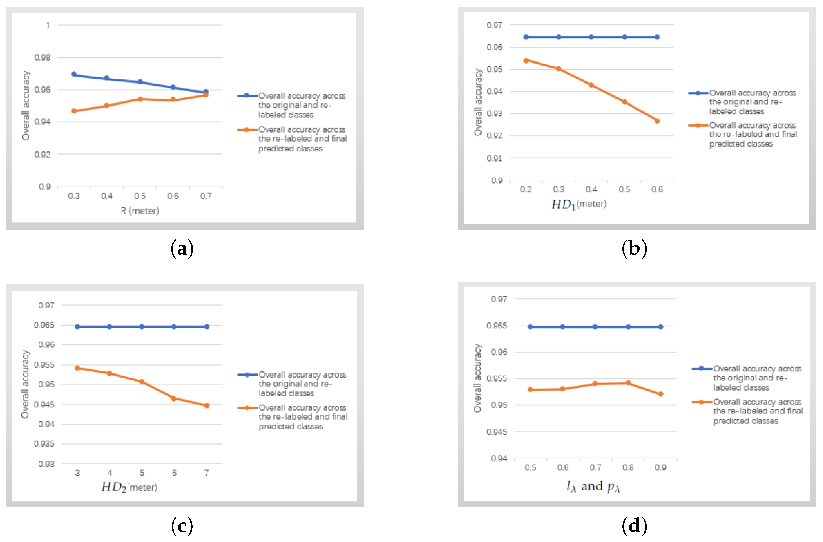
Figure 7 shows the two overall accuracies of the proposed approach tested by the training file of the Paris-Rue-Madame dataset [31] versus the variation of above parameters. The blue line shows the OA across the original and re-labeled classes. The orange line shows the OA across the re-labeled and the final predicted classes. The term re-labeled class and final predicted class will be explained in detail in Section 3.4. In Figure 7a, two overall accuracies are both larger than 94%, and the optimal point is located at R = 0.5 m. The optimal points in Figure 7b–d are respectively located at $H{D}_1$ = 0.2 m, $H{D}_2$ = 3 m, and $l_{\lambda }$ = $p_{\lambda }$ = 0.8. The following parameters of all experiments in the training process are set to be: R = 0.5 m, $H{D}_1$ = 0.2 m, $H{D}_2$ = 3 m, and $l_{\lambda }$ = $p_{\lambda }$ = 0.8. It is worth noting that overall accuracies keep stable in three blue lines of Figure 7b–d as R all is fixed at 0.5 m.

3.4. Result Analysis: Paris-Rue-Madame Dataset

The dataset contains two PLY files with 10 million points each. Each file contains a list of (X, Y, Z, reflectance, label, class) points, where class determines the object category. This database contains 642 objects categorized in 26 classes, which are further organized into three classes as shown in

Table 2. Three classes and the number of points in the Paris-Rue-Madame database. (NoPs: Number ofpoints).

	NoPs	NoPs
Class Name	First File	Second File
Others	897,524	1,099,746
Facade	4,769,417	5,209,018
Ground	4,333,059	3,691,236
Total	10,000,000	10,000,000

. The first file is chosen for training and the second file is for testing in this paper.

3.4.1. The Feasibility of Fourier Fitting

FF is introduced in Section 2.2.2. The aim is to separate points of multiple object classes lying within a single block of the first segmentation. The feasibility of FF is tested by two steps. It contains (i) re-label the class for the entire sub-block as the class of points inside it by voting; (ii) compare the label changes for each point before and after re-labeling. Examples in Figure 4 already visually present the positive role of FF. Here the feasibility of FF on the training file of the Paris-Rue-Madame database are quantificationally demonstrated.

Table 3. Overall results across the original and re-labeled classes on training file of the Paris-Rue-Madame database. O-xxx: Original-xxx. R-xxx: Relabeled-xxx. OA: overall accuracy.

Class	R-Others	R-Facade	R-Ground	Precision
O-Others	809,775	1288	86,461	0.9022
O-Facade	2640	4,751,876	14,901	0.9963
O-Ground	91,020	157,935	4,084,104	0.9425
Recall	0.8963	0.9676	0.9758
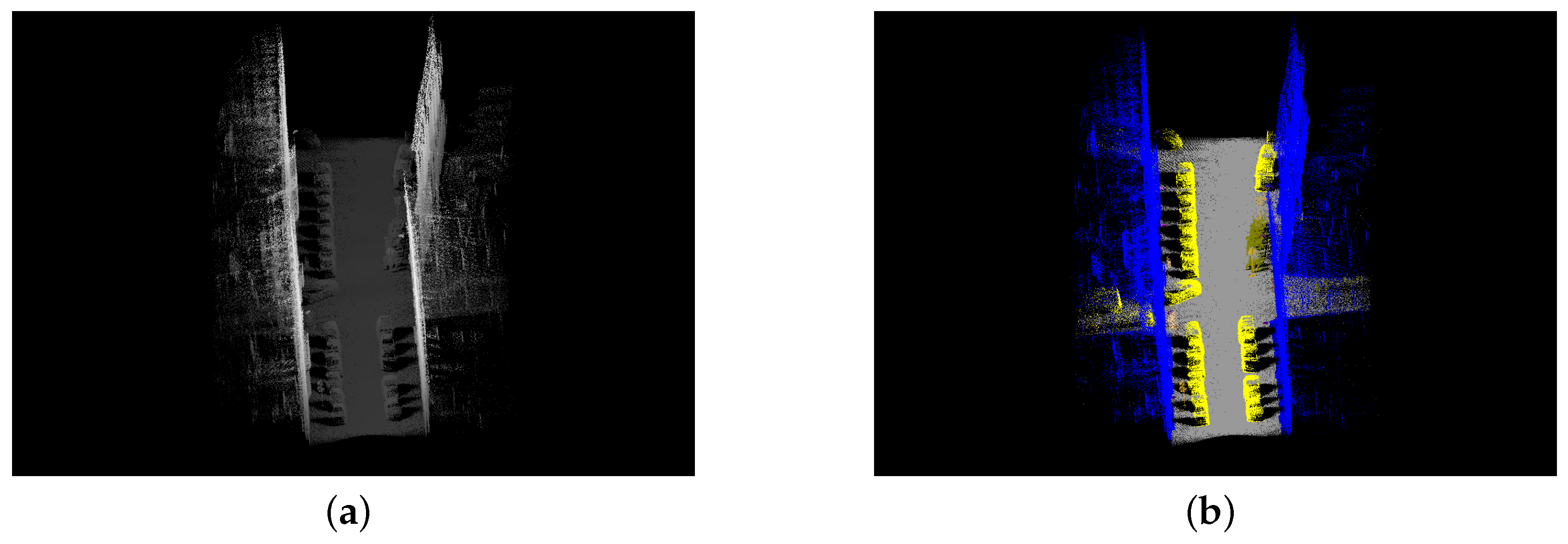
OA				0.9646

shows statistical results of re-labeling on the training file of Paris-Rue-Madame database. The OA is 96.46%. Most points of three classes still stay in the original classes. The error rate of re-labeling is less than 0.05, which means that FF could adaptively group points of the same class into the same sub-block. Figure 8 shows the training file of the Paris-Rue-Madame database before and after re-labeling. Because of the low error rate, two sub-figures in Figure 8 looks almost the same.

3.4.2. End-To-End Match

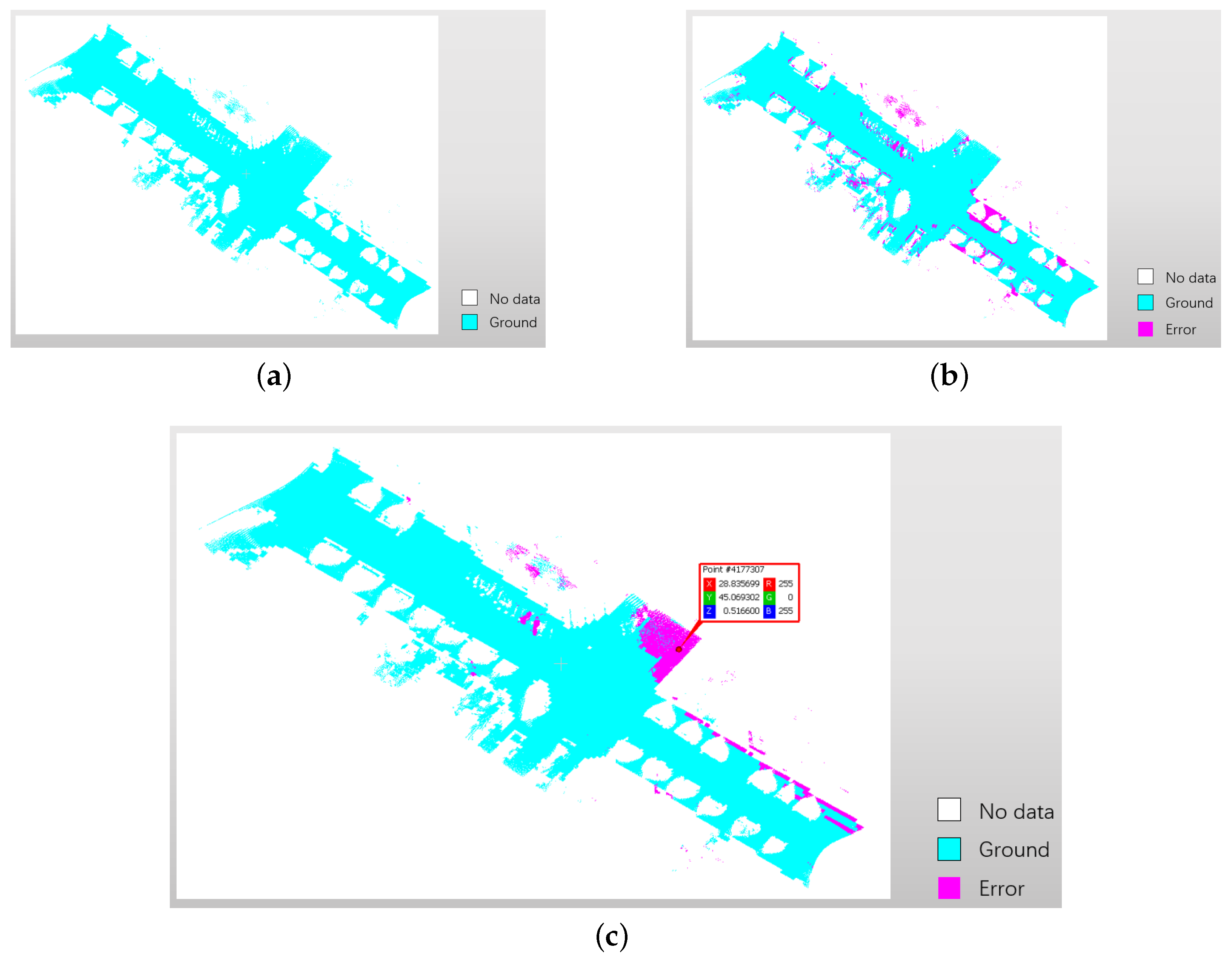
Section 2.4 states the significance behind the combinations of made-up labels. The section presents how to build the end-to-end match with this significance. Based on the knowledge, the first match of end-to-end is between class Ground and the combinations $[0,\ast ]$ (∗ means all made-up labels at the second segmentation, including “0” for planarity, “1” for linearity and “2” for scattering). Figure 9 shows the comparison of the filtering results of ground points between the proposed method and CloudCompare software. Figure 9b shows the errors scattered around the boundaries of different objects by CloudCompare software. In Figure 9c, the main mistakes of the proposed method locate within the area where the height of points is over 0.2 meter. In the red box of Figure 9c, Z means the physical height of the point is 0.516600 m.

Table 4. The comparison of ground point filtering with precision and recall between CloudCompare software and the proposed method.

	The CloudCompare	The Proposed Method
Precision	0.9738	0.9856
Recall	0.9201	0.9240

shows the comparison of ground point filtering with precision and recall between these two methods. The proposed method performs better on both precision and recall. Considering the advantages and disadvantages of these two methods for ground point filtering, the combination of these two methods will be used to improve the filtering result of ground points in future work.

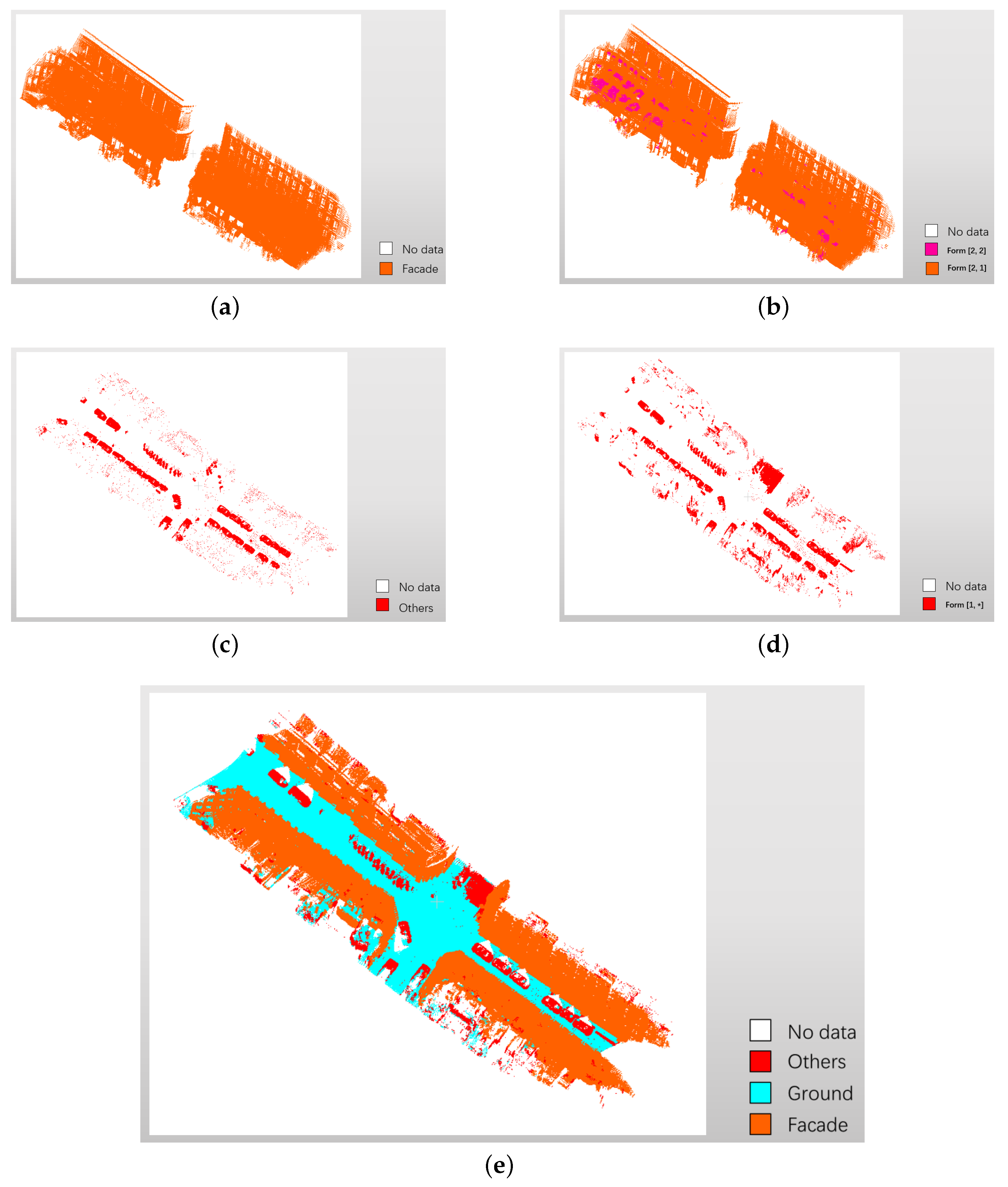
The ground truth of class Facade and Others and point clouds in terms of the corresponding combinations are compared in Figure 10. Figure 10a presents the ground truth of facade points in color orange, and Figure 10b shows the points in combinations $[2,1]$ and $[2,2]$. There are no sub-blocks in the form of $[2,0]$ for the training file of the Paris-Rue-Madame database. The main body of class Facade is colored in orange ($[2,1]$). Points in color rosy red ($[2,2]$) are attachments of facade, which also belong to class Facade. Figure 10c presents the ground truth of class Others in color red. Points of the combinations $[1,\ast ]$ (∗ means all made-up labels at the second segmentation, including “0” for planarity, “1” for linearity and “2” for scattering) are displayed in Figure 10d. Figure 10e gives the whole view of final classification result.

Finally, the knowledge-based end-to-end match is built from the combinations of made-up labels to three original classes: the combinations $[0,\ast ]$ matches class Ground, the combinations $[2,\ast ]$ matches class Facade, and the combinations $[1,\ast ]$ matches class Others.

Table 5. Overall results across the re-labeled and final predicted classes of the training file of Paris-Rue-Madame database. P-xxx: Predicted-xxx.

Class	P-Others	P-Facade	P-Ground	Precision
R-Others	602,111	8810	292,514	0.6665
R-Facade	50,636	4,813,912	46,551	0.9820
R-Ground	35,395	24,997	4,125,074	0.9856
Recall	0.8750	0.9930	0.9240
OA				0.9541

gives the overall results across the re-labeled and final predicted classes of the training file of Paris-Rue-Madame database by the end-to-end rule. The entry at the (i + 1)-th row and the (j + 1)-th column denotes the number of points of the re-labeled class of corresponding row that are classified as the class of corresponding column, $i,j=1,2,3$. The OA is 95.41%. The proposed method performs well on class Facade with both precision and recall. The street from Rue Madame slopes slightly. Part points of class Others located in low terrain easily confuse with points of class Ground. In Table 5, 292,514 points of class Others are misclassified into class Ground. In reverse, 35,395 points of class Ground are misclassified into class Others.

3.4.3. Performance Test

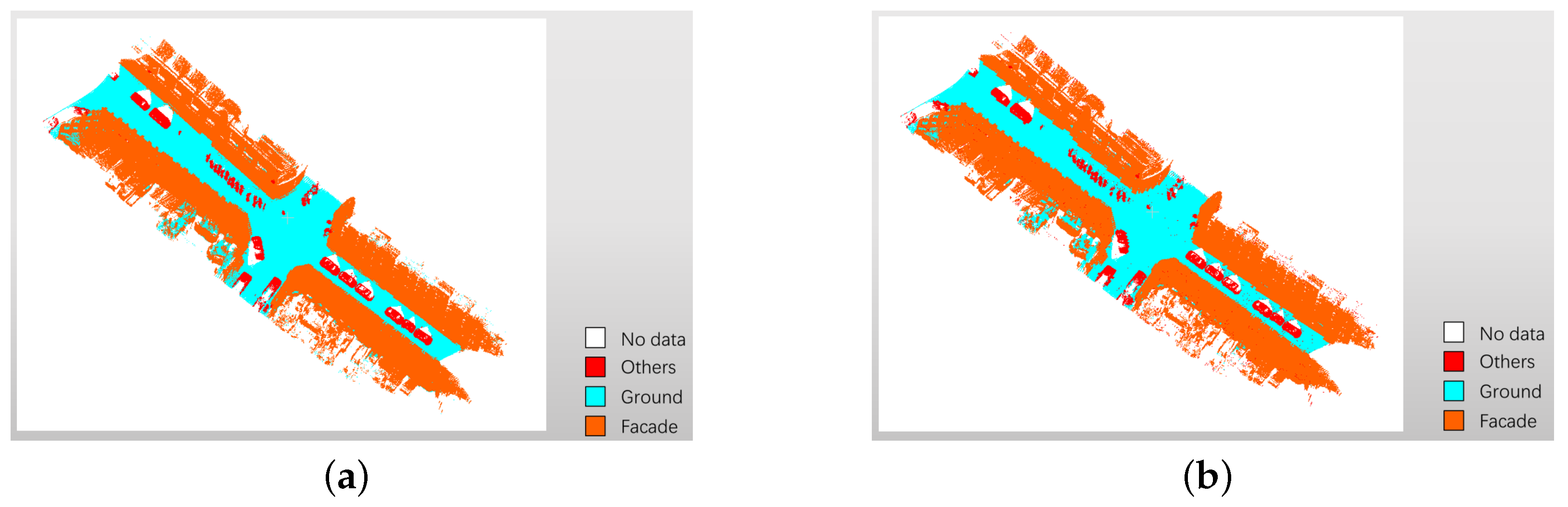
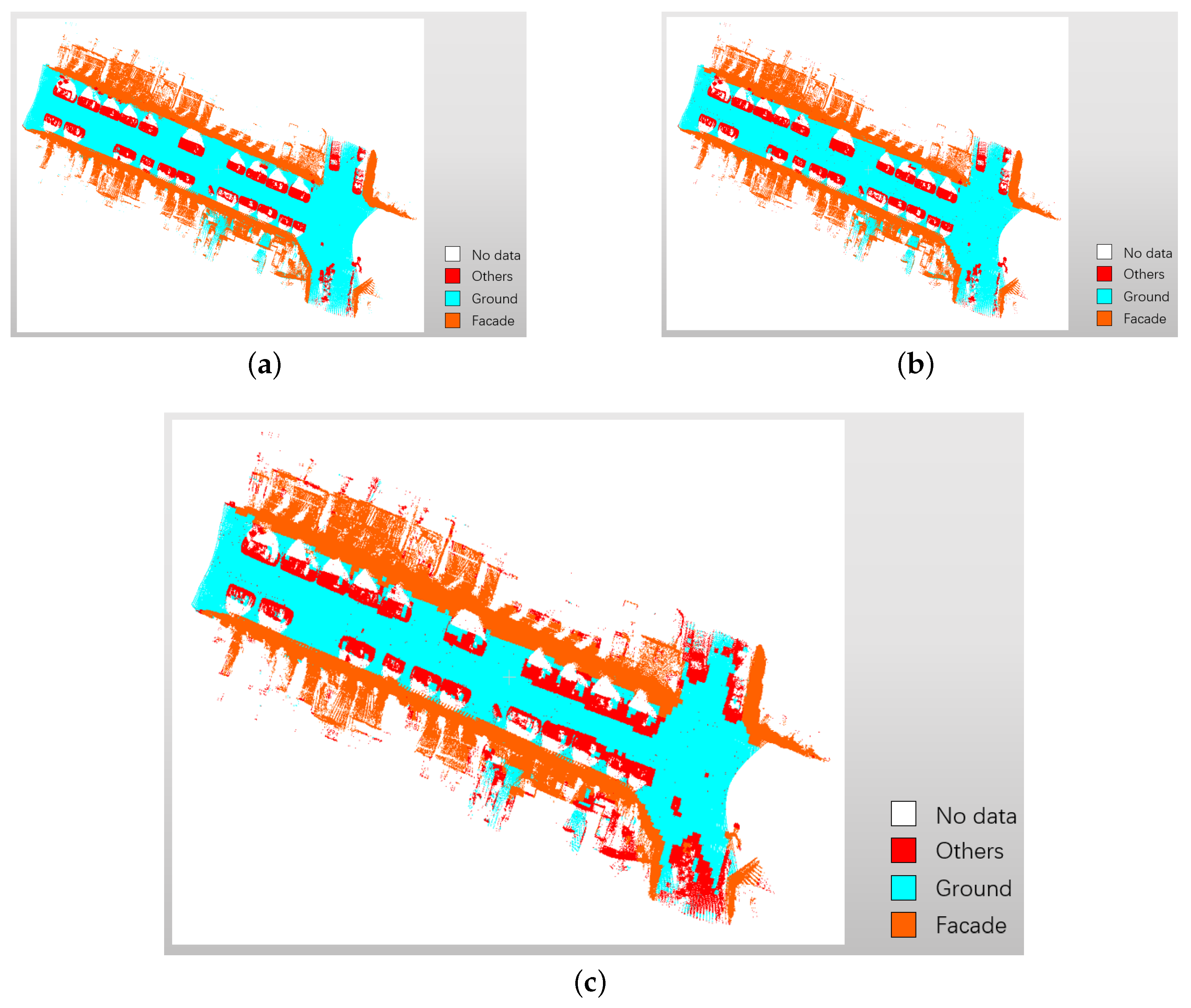
The second file of the Paris-Rue-Madame database is used as a test.

Table 6. Overall results across the original and re-labeled classes on test file of the Paris-Rue-Madamedatabase.

Class	R-Others	R-Facade	R-Ground	Precision
Others	1,027,226	6564	65,956	0.9341
Facade	1914	5,198,408	8696	0.9980
Ground	21,166	165,372	3,504,698	0.9495
Recall	0.9780	0.9680	0.9791
OA				0.9730

and

Table 7. Overall results across the re-labeled and final predicted classes on test file of the Paris-Rue-Madame database.

Class	P-Others	P-Facade	P-Ground	Precision
R-Others	954,408	14,940	80,958	0.9087
R-Facade	63,126	5,301,491	5727	0.9872
R-Ground	231,687	81,848	3,265,815	0.9124
Recall	0.7640	0.9821	0.9841
OA				0.9522

separately show the overall results across the classes. The OA is 97.30% and 95.22% respectively. In Table 7, misclassification mainly happens between class Ground and Others as slight slope in the street of the 6th Parisian district.

Table 8. A comparison with the results [36] in the same dataset [31].

	Weinmann et al. [36]		The Proposed Method
	Precision	Recall	Precision	Recall
Facade	0.964	0.958	0.987	0.982
Ground	0.960	0.911	0.912	0.984

shows a comparison with the results [36] in the same dataset [31]. Considering the difference of class defining, the results of two same classes Ground and Facade are selected out to make a comparison. The proposed method performs better expect for precision of class Ground. The expected use case in the paper is 3D city maps, there is no need to focus on improving the accuracy of misclassification. Figure 11 show the test file before and after re-labeling, and the final classification result. It displays that the proposed method could performs on object classification of these three classes. The red area on the lower right in Figure 11c shows the mistake of ground point filtering.

In addition, the algorithm runs on a computer with Intel(R) Core(TM) I7-7700HQ CPU @ 2.80 GHz with 4 cores, RAM 16.0 GB. The programming language is in MATLAB. The computation time for the complete test process is less than 80 min.

3.5. Result Analysis: Cyclomedia Dataset

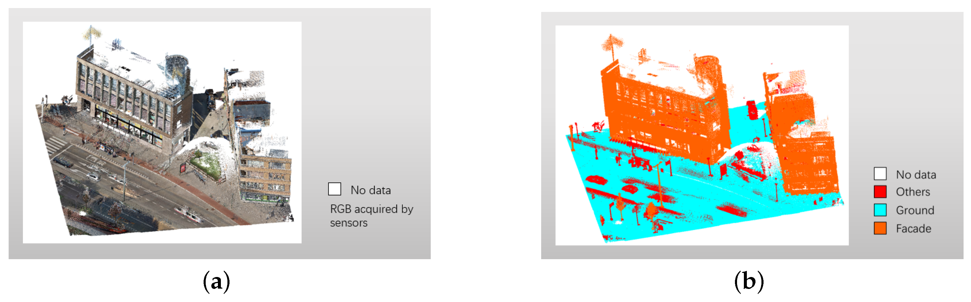
In the section, the proposed method is applied to the Cyclomedia dataset which does not contain label information. In 2007, West et al. proposed the concept of transfer learning [37], “a research problem in machine learning that focuses on storing knowledge gained while solving one problem and applying it to a different but related problem.” A simple example is that the knowledge gained while learning to identify cars could apply when trying to identify trucks. Here, the knowledge and the rule of end-to-end match of urban objects in the Paris-Rue-Madame database is transferred applying to the Cyclomedia dataset. Figure 12 gives the original scene and the final result of the Cyclomedia dataset. The parameter values are set to be: R = 0.5 m, $H{D}_1$ = 0.5 m, $H{D}_2$ = 5 m, and $L_{\lambda }=P_{\lambda }=0.7$. The process of parameter setting for the Cyclomedia dataset is the same to which of the Paris-Rue-Madame dataset. As the scenes change from Rue Madame to Schiedam, the parameters differ.

The color of points in Figure 12a is the original RGB value acquired by sensors. In Figure 12b, most points of classes Facade and Ground are properly classified. However, part of trees and high-poles are confused with buildings. The main cause of the confusion is that $\Delta h$ of this part of trees and high-poles in the Cyclomedia dataset is larger than $H{D}_2$. According to the rule of end-to-end match in Section 2.4, these parts are misclassified as class Facade. In addition, it contains 6,332,595 points in the Cyclomedia dataset, and the computation time for the complete procedure is approximately one hour.

3.6. Discussion

To create a comfortable life environment, almost objects in urban city exist based on human knowledge. In other words, basic pattern of artificial objects in public places is similar in different cities and countries. Height difference and geometrical eigen-features just reflect these similar characteristics of objects. In the paper, the knowledge-based end-to-end match is built between the combinations of made-up labels and three defined classes: the combination $[0,\ast ]$ matches class Ground; the combination $[2,\ast ]$ matches class Facade; the combination $[1,\ast ]$ matches class Others. Taking the Cyclomedia dataset as an example to explain the second match. Statistical results show that a 3D block is segmented into five 3D sub-blocks in most cases, and the physical height of facades in the Cyclomedia dataset is higher than 15 meters. The average height of each sub-block is more than 3 meters. Then it is easy to imagine that the shape of points in sub-blocks of class Facade accompanying with the tile size 0.5 m looks linear. That is why the main body of class Facade is colored in orange ($[2,1]$).

It is worth noting three special situations for correcting part made-up labels of 3D sub-blocks.

• Situation I: small h but large $\Delta h$

This situation suits for the ground points, which overlap with other objects on the plane of x and y coordinates during the first segmentation. Generally, for the sub-blocks, which only contain ground points after the two-step segmentation, their first made-up labels are corrected by comparing the physical height of points inside them with threshold $H{D}_1$.

• Situation II: large h but small $\Delta h$

The height difference $\Delta h$ of the attachment of facades probably is lower than $H{D}_1$. As the same operation as in situation I, the physical height of points of 3D blocks in the form of $[0,\ast ]$ is compared with threshold $H{D}_2$ to adjust their first made-up labels.

• Situation III: majority

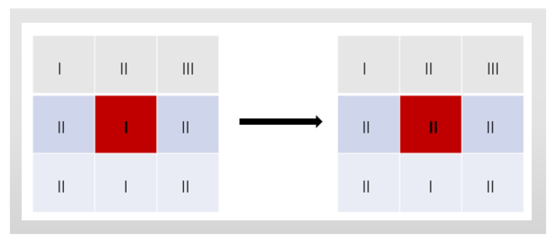
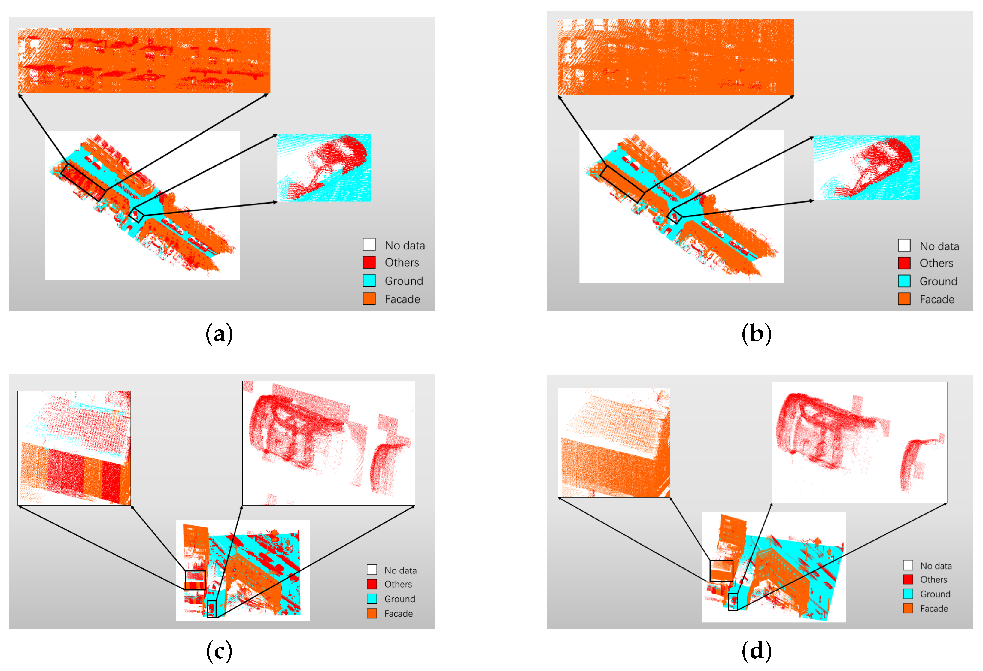
It is possible that there are points of multiple object classes lying within a single sub-block after the two-step segmentation. It is common at the boundary of multiple objects. For example, it mainly contains ground points in a 3D sub-block, mixing up with a few points of a car. $H{D}_1$ of the sub-block is impacted by these car points, resulting the misclassification of these ground points. The problem is solved by voting the neighborhoods of the 3D sub-block. A 2D example is given in Figure 13. Centered grid C is labeled by symbol I, the labels of its neighborhoods are counted. By voting, the grid C is labeled by symbol II. In the rare case where two or more symbols have equal number, just a random one is picked. The local correction of the Paris-Rue-Madame database and the Cyclomedia dataset are shown in Figure 14. Figure 14a,c show the points mixture of multiple objects. Figure 14b,d show the modified results.

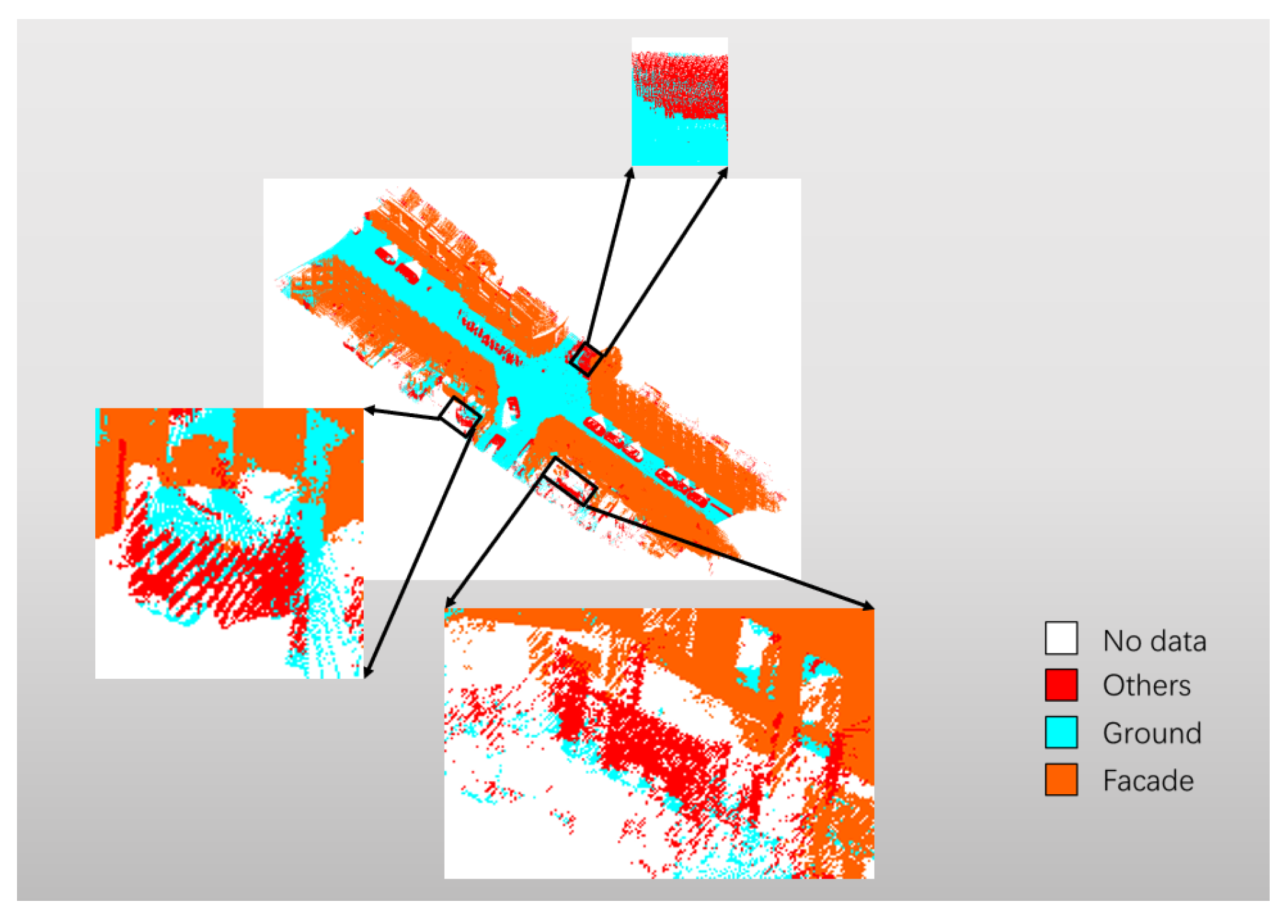
However, due to the complexity of urban scenes and the limitation of defined features, there are still some confusions in Figure 15. While more features are defined, these three defined classes could be segregated into a multi-class (>3) problem to classify complex objects. There will be a unique end-to-end match between one combination of made-up labels and one object. What is more, these discriminating features can be used in other point cloud applications. For instance, they can help to label raw datasets and generate training samples. In addition, the proposed method has good performance at the cost of resetting parameters while applying in different urban scenes. Fortunately, the computation time is not a burden because the proposed approach does not need heavy training process.

4. Conclusions and Future Work

In this paper, an adaptive end-to-end approach based on knowledge for object classification is proposed. In comparison to common classification methods which need massive training samples, only basic knowledge of objects in urban scenes is needed. FF is used to adaptively produce sub-blocks at the second segmentation. Overall accuracies across the original and re-labeled classes are both over 96% as in Table 3 and Table 6, which demonstrates the feasibility of FF. Two types of features, height difference ($\Delta h$) and geometrical eigen-features, are defined to provide made-up labels for points of sub-blocks. The final result on the test file of the Paris-Rue-Madame dataset is 95.22%. The proposed approach is also tested on the Cyclomedia dataset. In summary, qualitative and quantificational experimental results show the proposed approach has promising performance for objects classification in various urban scenes. Additionally, the proposed approach can save lots of the computation time without heavy training process.

In future work, it is the core to define more discriminating features for classifying confused objects into right classes. For instance, part of trees and high pole-likes are mixed with facades, point density will be an option for this problem. Generally, for a “linear” object, points of which should be close in space and have the same/similar principal direction. For a “planar” object, points of which should be close in space and have the same/similar normal vector. Also, for a “spherical” object, points of which should be close in space but without the constraints of principle direction and normal vector. Therefore, in the next step, considering improving the performance in confused objects, region growing [38] with these three features is a good option. In addition, the thresholds $H{D}_1$ and $H{D}_2$ fixed in the paper, can be flexibly adjusted based on the diverse objects in urban scenes.

References

- Dimitrakopoulos, G.; Demestichas, P. Intelligent transportation systems. IEEE Veh. Technol. Mag. 2010, 5, 77–84. [Google Scholar] [CrossRef]
- Levinson, J.; Askeland, J.; Becker, J.; Dolson, J.; Held, D.; Kammel, S.; Kolter, J.Z.; Langer, D.; Pink, O.; Pratt, V.; et al. Towards fully autonomous driving: Systems and algorithms. In Proceedings of the 2011 IEEE Intelligent Vehicles Symposium (IV), Baden-Baden, Germany, 5–9 June 2011; pp. 163–168. [Google Scholar]
- Aijazi, A.K.; Checchin, P.; Trassoudaine, L. Segmentation based classification of 3D urban point clouds: A super-voxel based approach with evaluation. Remote Sens. 2013, 5, 1624–1650. [Google Scholar] [CrossRef]
- Soilán, M.; Truong-Hong, L.; Riveiro, B.; Laefer, D. Automatic extraction of road features in urban environments using dense ALS data. Int. J. Appl. Earth Obs. Geoinf. 2018, 64, 226–236. [Google Scholar] [CrossRef] [Green Version]
- Babahajiani, P.; Fan, L.; Gabbouj, M. Object recognition in 3d point cloud of urban street scene. In Asian Conference on Computer Vision; Springer: Cham, Switzerland, 2014; pp. 177–190. [Google Scholar]
- Zheng, M.; Lemmens, M.; van Oosterom, P. Classification of mobile laser scanning point clouds from height features. Int. Arch. Photogramm. Remote Sens. Spat. Inf. Sci. 2017, 42, 321–325. [Google Scholar] [CrossRef]
- Zheng, M.; Lemmens, M.; van Oosterom, P. Classification of mobile laser scanning point clouds of urban scenes exploiting cyclindrical neighbourhoods. Int. Arch. Photogramm. Remote Sens. Spat. Inf. Sci. 2018, 42, 1225–1228. [Google Scholar] [CrossRef]
- Weinmann, M.; Jutzi, B.; Hinz, S.; Mallet, C. Semantic point cloud interpretation based on optimal neighborhoods, relevant features and efficient classifiers. ISPRS J. Photogramm. Remote Sens. 2015, 105, 286–304. [Google Scholar] [CrossRef]
- Lehtomäki, M.; Jaakkola, A.; Hyyppä, J.; Lampinen, J.; Kaartinen, H.; Kukko, A.; Puttonen, E.; Hyyppä, H. Object classification and recognition from mobile laser scanning point clouds in a road environment. IEEE Trans. Geosci. Remote Sens. 2016, 54, 1226–1239. [Google Scholar] [CrossRef]
- Qi, C.R.; Yi, L.; Su, H.; Guibas, L.J. Pointnet++: Deep hierarchical feature learning on point sets in a metric space. Adv. Neural Inf. Process. Syst. 2017, 5105–5114. [Google Scholar]
- Wang, L.; Huang, Y.; Shan, J.; He, L. MSNet: Multi-Scale Convolutional Network for Point Cloud Classification. Remote Sens. 2018, 10, 612. [Google Scholar] [CrossRef]
- Gunst, M. Automatic Extraction of Roads from SPOT Images; Faculty of Geodesy; TU Delft: Delft, The Netherlands, 1991. [Google Scholar]
- De Gunst, M.E.; Lemmens, M. Automatized updating of road databases from scanned aerial photographs. Int. Arch. Photogramm. Remote Sens. Spat. Inf. Sci. 1992, 29, 477–484. [Google Scholar]
- Vosselman, G.; de Gunst, M. Updating road maps by contextual reasoning. In Automatic Extraction of Man-Made Objects from Aerial and Space Images (II); Springer: Basel, Switzerland, 1997; pp. 267–276. [Google Scholar]
- Zhang, C.; Baltsavias, E.P. Knowledge-based image analysis for 3D edge extraction and road reconstruction. ISPRS Int. Soc. Photogramm. Remote Sens. 2000, 33, 1008–1015. [Google Scholar]
- Lemmens, M. On a knowledge-based approach to the classification of mobile laser scanning point clouds. Int. Arch. Photogramm. Remote Sens. Spat. Inf. Sci. 2018, XLII-4, 343–349. [Google Scholar] [CrossRef]
- Rabbani, T.; Van Den Heuvel, F.; Vosselmann, G. Segmentation of point clouds using smoothness constraint. Int. Arch. Photogramm. Remote Sens. Spat. Inf. Sci. 2006, 36, 248–253. [Google Scholar]
- Vosselman, G.; Gorte, B.G.; Sithole, G.; Rabbani, T. Recognising structure in laser scanner point clouds. Int. Arch. Photogramm. Remote Sens. Spat. Inf. Sci. 2004, 46, 33–38. [Google Scholar]
- Douillard, B.; Underwood, J.; Kuntz, N.; Vlaskine, V.; Quadros, A.; Morton, P.; Frenkel, A. On the segmentation of 3D LIDAR point clouds. In Proceedings of the 2011 IEEE International Conference on Robotics and Automation (ICRA), Shanghai, China, 9–13 May 2011; pp. 2798–2805. [Google Scholar]
- Zhang, Z.; Zhang, L.; Tong, X.; Mathiopoulos, P.T.; Guo, B.; Huang, X.; Wang, Z.; Wang, Y. A multilevel point-cluster-based discriminative feature for ALS point cloud classification. IEEE Trans. Geosci. Remote Sens. 2016, 54, 3309–3321. [Google Scholar] [CrossRef]
- Yang, B.; Dong, Z.; Zhao, G.; Dai, W. Hierarchical extraction of urban objects from mobile laser scanning data. ISPRS J. Photogramm. Remote Sens. 2015, 99, 45–57. [Google Scholar] [CrossRef]
- Pu, S.; Vosselman, G. Automatic extraction of building features from terrestrial laser scanning. Int. Arch. Photogramm. Remote Sens. Spat. Inf. Sci. 2006, 36, 25–27. [Google Scholar]
- Biosca, J.M.; Lerma, J.L. Unsupervised robust planar segmentation of terrestrial laser scanner point clouds based on fuzzy clustering methods. ISPRS J. Photogramm. Remote Sens. 2008, 63, 84–98. [Google Scholar] [CrossRef]
- Trevor, A.J.; Gedikli, S.; Rusu, R.B.; Christensen, H.I. Efficient organized point cloud segmentation with connected components. In Proceedings of the Semantic Perception Mapping and Exploration (SPME), Karlsruhe, Germany, 5 May 2013. [Google Scholar]
- Altantsetseg, E.; Muraki, Y.; Matsuyama, K.; Konno, K. Feature line extraction from unorganized noisy point clouds using truncated Fourier series. Vis. Comput. 2013, 29, 617–626. [Google Scholar] [CrossRef]
- Jonsson, P.; Eklundh, L. Seasonality extraction by function fitting to time-series of satellite sensor data. IEEE Trans. Geosci. Remote Sens. 2002, 40, 1824–1832. [Google Scholar] [CrossRef]
- Dong, W.; Lan, J.; Liang, S.; Yao, W.; Zhan, Z. Selection of LiDAR geometric features with adaptive neighborhood size for urban land cover classification. Int. J. Appl. Earth Obs. Geoinf. 2017, 60, 99–110. [Google Scholar] [CrossRef]
- Li, D.; Elberink, S.O. Optimizing detection of road furniture (pole-like objects) in mobile laser scanner data. ISPRS Ann. Photogramm. Remote Sens. Spat. Inf. Sci. 2013, 1, 163–168. [Google Scholar] [CrossRef]
- Weinmann, M.; Jutzi, B.; Mallet, C. Feature relevance assessment for the semantic interpretation of 3D point cloud data. ISPRS Ann. Photogramm. Remote Sens. Spat. Inf. Sci. 2013, 5, 313–318. [Google Scholar] [CrossRef]
- Chehata, N.; Guo, L.; Mallet, C. Airborne lidar feature selection for urban classification using random forests. Int. Arch. Photogramm. Remote Sens. Spat. Inf. Sci. 2009, 38, 207–212. [Google Scholar]
- Serna, A.; Marcotegui, B.; Goulette, F.; Deschaud, J.E. Paris-rue-Madame database: A 3D mobile laser scanner dataset for benchmarking urban detection, segmentation and classification methods. In Proceedings of the 4th International Conference on Pattern Recognition Applications and Methods (ICPRAM 2014), Angers, France, 6–8 March 2014. [Google Scholar]
- Baron Fourier, J.B.J. The Analytical Theory of Heat; The Cambridge University Press: Cambridge, UK, 1878. [Google Scholar]
- Gross, H.; Thoennessen, U. Extraction of lines from laser point clouds. Int. Arch. Photogramm. Remote Sens. Spat. Inf. Sci. 2006, 36, 86–91. [Google Scholar]
- Demantke, J.; Mallet, C.; David, N.; Vallet, B. Dimensionality based scale selection in 3D lidar point clouds. Int. Arch. Photogramm. Remote Sens. Spat. Inf. Sci. 2011, 38, W12. [Google Scholar] [CrossRef]
- Lin, C.H.; Chen, J.Y.; Su, P.L.; Chen, C.H. Eigen-feature analysis of weighted covariance matrices for LiDAR point cloud classification. ISPRS J. Photogramm. Remote Sens. 2014, 94, 70–79. [Google Scholar] [CrossRef]
- Weinmann, M.; Jutzi, B.; Mallet, C. Semantic 3D scene interpretation: A framework combining optimal neighborhood size selection with relevant features. ISPRS Ann. Photogramm. Remote Sens. Spat. Inf. Sci. 2014, 2, 181. [Google Scholar] [CrossRef]
- West, J.; Ventura, D.; Warnick, S. Spring Research Presentation: A Theoretical Foundation for Inductive Transfer; College of Physical and Mathematical Sciences, Brigham Young University: Provo, UT, USA, 2007. [Google Scholar]
- Adams, R.; Bischof, L. Seeded region growing. IEEE Trans. Pattern Anal. Mach. Intell. 1994, 16, 641–647. [Google Scholar] [CrossRef]
Figure 1.
The proposed workflow.
Figure 2.
The relationship between physical height and the number of points.
Figure 3.
Figure 4.
Example-based FF during the second segmentation. The left is the relationship between the physical height and the number of points (a,c,e,g), and the right is the corresponding fitting curve (b,d,f,h).
Figure 5.
Surjective relation from made-up label combinations to three defined classes.
Figure 6.
3D point clouds colored by its available fields from Rue Madame. (a) physical height (Z coordinate); (b) Object class.
Figure 7.
The overall accuracies (OA) of the proposed approach tested by the training file of the Paris-Rue-Madame dataset versus the variation of above parameters. (a) OA versus R; (b) OA versus ; (c) OA versus ; (d) OA versus and .
Figure 8.
The training file of the Paris-Rue-Madame database before and after re-labeling. (a) original scene; (b) the re-labeled scene.
Figure 9.
The comparison of the filtering results of ground points between the proposed method and CloudCompare software. (a) original scene; (b) CloudCompare software; (c) the proposed method.