Hyperspectral Anomaly Detection via Dictionary Construction-Based Low-Rank Representation and Adaptive Weighting


School of Physics and Optoelectronic Engineering, Xidian University, Xi’an 710071, China
*
Authors to whom correspondence should be addressed.
Remote Sens. 2019, 11(2), 192; https://0-doi-org.brum.beds.ac.uk/10.3390/rs11020192
Submission received: 13 December 2018
/
Revised: 16 January 2019
/
Accepted: 17 January 2019
/
Published: 19 January 2019
(This article belongs to the Special Issue Remote Sensing for Target Object Detection and Identification)
Abstract
:Anomaly detection (AD), which aims to distinguish targets with significant spectral differences from the background, has become an important topic in hyperspectral imagery (HSI) processing. In this paper, a novel anomaly detection algorithm via dictionary construction-based low-rank representation (LRR) and adaptive weighting is proposed. This algorithm has three main advantages. First, based on the consistency with AD problem, the LRR is employed to mine the lowest-rank representation of hyperspectral data by imposing a low-rank constraint on the representation coefficients. Sparse component contains most of the anomaly information and can be used for anomaly detection. Second, to better separate the sparse anomalies from the background component, a background dictionary construction strategy based on the usage frequency of the dictionary atoms for HSI reconstruction is proposed. The constructed dictionary excludes possible anomalies and contains all background categories, thus spanning a more reasonable background space. Finally, to further enhance the response difference between the background pixels and anomalies, the response output obtained by LRR is multiplied by an adaptive weighting matrix. Therefore, the anomaly pixels are more easily distinguished from the background. Experiments on synthetic and real-world hyperspectral datasets demonstrate the superiority of our proposed method over other AD detectors.
1. Introduction
In contrast to color and multispectral imagery, hundreds of narrow and contiguous spectral bands covering a wide range of wavelengths contained in hyperspectral imagery provide abundant spatial and spectral information about Earth observations [1,2]. Since each material has unique electromagnetic reflection characteristics at different wavelengths, their spectral information can be used for target detection [3]. According to the availability of prior knowledge about the target signatures, target detection can be divided into two categories: supervised and unsupervised [4]. Unsupervised target detection, known as anomaly detection (AD), has attracted a lot of attention over the last 20 years because it does not require any prior information about the spectral characteristics of targets that are usually difficult to obtain [5]. Moreover, it does not need radiation calibration and atmospheric absorption compensation [6].
Anomalies refer to the small objects with low probability of occurrence and whose spectra are significantly different from the main background. AD can be regarded as a binary classification problem designed to separate the background class and the anomaly class automatically [7]. In recent years, many AD methods have been proposed, and among them, the Reed-Xiaoli (RX) detector is the most well-known method based on statistical modeling [8]. It uses the probability density functions of the multivariate normal distribution to measure the probability of the detected pixel to be background, and its solution is the Mahalanobis distance between the spectrum of the detected pixel and the background. It has two versions: global RX (GRX) and local RX (LRX). Specifically, GRX estimates background statistics from the full image scene, whereas the background in LRX is estimated from the local neighborhood of the detected pixel using a dual-window strategy [9]. However, the background composition of HSI is usually complicated and nonhomogeneous in practical, so a single multivariate normal distribution is generally unsuitable for describing the background [10]. Moreover, the anomaly contamination in background statistics (background mean and covariance matrix) is another potential problem with RX. Based on these two shortcomings, several improved RX-based AD methods have been proposed. For example, the Gaussian mixture model-based detector [11] uses a mixture of multivariate Gaussian distributions to model the multimode background to capture the complexity of the background. The cluster-based anomaly detector (CBAD) [12] applies a clustering technique to divide the dataset into some homogeneous clusters and then implements RX on each cluster. The subspace RX (SSRX) [13] performs RX on a finite number of principal components obtained by principal component analysis (PCA), thereby reducing computational cost and improving the separability of background and anomalies. Due to the rich nonlinear information among the inter-bands of HSI, kernel-RX (KRX) [14] and support vector data description (SVDD) [15] are applied to project the original data into an infinite high-dimensional space through a kernel function. Cluster KRX (CKRX) [16], as an improved version of KRX, groups background pixels into clusters and then applies a fast eigendecomposition algorithm to generate anomaly indexes. It significantly reduces computation time by replacing each pixel with its cluster center. There are some AD methods trying to mitigate anomaly contamination for a pure estimation of the background. For example, the random-selection-based anomaly detector (RSAD) [17] applies a selection procedure several times to choose some representative background pixels. The blocked adaptive computationally efficient outlier nominator (BACON) detector [18] uses the subsets of the entire HSI to iteratively update a stable and robust background to suppress anomaly contamination in the background estimation.
With the development of representation theory in recent years, some representation-based methods have been successfully applied to AD. They sidestep the difficulty of modeling the complicated distribution of background in statistics-based methods. The sparse representation-based detector (SRD) [19] assumes that the spectrum of a pixel can be sparsely represented by a linear combination of a few sparse coefficients with respect to a background dictionary, and the reconstruction error is used to measure the anomaly response. The collaborative representation-based detector (CRD) [20] is based on the fact that background pixels can be well approximated by their spatial neighborhoods, whereas anomalies cannot. In addition to CRD, there are some other methods to incorporate spatial or feature information into detection and classification. In [21], during the recovery of sparse vector in sparse representation, two different approaches are proposed to incorporate the contextual information of HSI to improve the classification performance. In [22], the joint sparsity model is extended to a feature space induced by a nonlinear kernel function for improving the discrimination between background and targets. In this case, the spectral, spatial, and feature information are jointly used.
Recently, low-rank-based methods have drawn much attention and been applied to AD. It exploits the intrinsic low-rank property of background and the sparse property of anomalies [23]. It also does not require modeling the distribution of complex background. For instance, robust principal component analysis (RPCA) [24] performs detection by decomposing HSI data into a low-rank background matrix and a sparse anomaly matrix. However, the sparse matrix obtained is always contaminated by isolated noise, thus causing some false alarm points [25]. As an improvement, low-rank and sparse matrix decomposition (LRaSMD) [26] extracts noise from the valuable signals, and then further separates the low-rank background and sparse anomalies. The anomaly detector in [27] first extracts some source components by using the unmixing operation, and then identifies the components that are sparse and have the largest accumulated distance from other components. The optimization problem is converted to a low-rank matrix decomposition problem and can be solved. Low-rank representation (LRR) [28] assumes that the HSI data lie in multiple subspaces and requires a dictionary to span the data space to separate the background and anomalies. Due to the mixed property of real-world datasets, the pixels of an HSI are usually drawn from multiple subspaces. Therefore, compared with RPCA and LRaSMD, LRR is theoretically more suitable for real HSI datasets by imposing l constraint on the sparse component [25]. In addition, the l constraint makes the background component unaffected by the column-wise sparse anomalies [29]. Some advanced LRR-based AD methods have been proposed in recent years and they improve the detection performance of LRR from different aspects. For example, the anomaly detector based on low-rank and learned dictionary (LRALD) in [23] constructs a dictionary from the whole image with a random selection process and then performs LRR. The abundance- and dictionary-based low-rank decomposition (ADLR) in [25] applies spectral unmixing to obtain some abundance maps that contains more distinctive features, and then constructs a dictionary based on the mean shift clustering, and finally performs LRR. The low-rank and sparse representation-based detector (LRASR) in [28] improves LRR through a sparsity-inducing regularization term and a cluster-based dictionary construction strategy. It can be found that all these methods build a reasonable dictionary and try to make the anomalies easier to be recognized. Dictionary construction is an important process in many HSI problems and there are many ways to implement it. [30] proposes an AD method based on sparse presentation through constructing multiple dictionaries to learn discriminative features. In each category, the representative spectra that can significantly enhance the difference between background and anomalies are selected.
In the original model of LRR, the entire input dataset is used as the dictionary to span the data space. However, due to the anomaly contamination in this dictionary, sparse anomalies cannot be effectively separated from the background component [23]. In addition, the heavy computational burden caused by large data size is also an important issue. In the LRR model based on randomly selected dictionary, there is no guarantee that the selected dictionary atoms contain all background categories. In this paper, taking into account the above issues, a novel AD algorithm via dictionary construction-based LRR and adaptive weighting is proposed. To better represent the background subspace and separate the anomaly component from the background, a background dictionary construction strategy based on the usage frequency of each dictionary atom for HSI reconstruction is adopted in LRR. To cover all background classes in the dictionary, the K-means clustering is first executed to divide the data into several clusters. Then, we estimate the background pixels in each cluster. It is based on the observation that if an atom has a high usage frequency for HSI reconstruction, it is more likely to be a background pixel [31]. Therefore, from the perspective of the usage frequency of the dictionary atoms used for HSI reconstruction in each cluster, we can obtain a reasonable estimation of the background dictionary, which can exclude anomaly contamination and contain all background categories. Furthermore, for further enhancing the response difference between the anomaly pixels and the background pixels, an adaptive weighting method based on the reconstruction residual of the entire data with respect to the background dictionary constructed above is proposed. The final anomaly response of each pixel is calculated by multiplying the value obtained through LRR by the weight. Compared with the existing LRR-based detectors, our proposed algorithm avoids the randomness brought by the random selection process (compared with LRALD), does not damage the physical structure of HSI (compared with ADLR), and needs less computation time than LRASR, which adds a sparsity-inducing regularization term to LRR. In addition, the distinction between background and anomalies can be significantly improved by our adaptive weighting method, which has not been used in other LRR-based algorithms. The main contributions of our proposed algorithm for AD can summarized as follows:
(1) Use of the LRR model. First, the LRR model is highly consistent with the hyperspectral AD problem and is therefore used in this paper. Second, the real-world HSIs are usually lying in multiple subspaces due to the presence of mixed pixels caused by insufficient sensor resolution [25]. The LRR model assumes that the data are in multiple subspaces by imposing l constraint on the sparse component, so it is suitable for real data. Third, the l constraint also makes the background unaffected by the column-wise sparse anomalies [29].
(2) Background dictionary construction strategy. To better separate the sparse anomalies from the background component and reduce the computational burden, a novel background dictionary is constructed by analyzing the usage frequency of the dictionary atoms for HSI reconstruction in each cluster. The dictionary is an excellent representation of the background subspace since it excludes anomaly contamination and covers all background categories. Therefore, the sparse component containing most of the anomaly information is extracted accurately.
(3) Adaptive weighting method. To further enhance the diversity between the background pixels and the anomaly pixels, an adaptive weighting method is introduced in our proposed algorithm by reusing the constructed background dictionary. By multiplying the results of LRR by the weights, the background and anomalies are more easily distinguished in the final detection map.
The rest of this paper is organized as follows. In Section 2, we briefly review the LRR model and its solution. In Section 3, the background dictionary construction strategy and adaptive weighting method in our proposed algorithm are described in detail. In Section 4, experimental results and analysis based on synthetic and real-world HSI datasets are provided. Finally, Section 5 concludes this paper.
2. Low-Rank Representation and Its Solution
In this section, we briefly introduce the consistency of the LRR model and the hyperspectral AD theory. Then the solution of LRR is provided. It plays a significant role in our proposed algorithm.
2.1. LRR Model for AD
There are several typical characteristics in HSIs. (1) Unlike anomaly pixels, there are strong correlations among the background pixels, i.e., the spectrum of a background pixel can be represented as a linear combination of some other background pixels [32]. (2) Anomalies occupy only a few pixels with a low probability of occurrence, that is, they are sparse spatially [33]. (3) Due to the limitation of the resolution of hyperspectral sensors, there are many mixed pixels in the real-world HSIs. Since the spectrum of each mixed pixel can be represented as a mixture of some pure materials (endmembers) and each endmember can be described in a subspace, all pixels in the HSI can be drawn from multiple subspaces [34]. The LRR model takes into account the above characteristics of HSI and is therefore very suitable for AD. The model of LRR is as follows:
where the HSI matrix is decomposed into a background component and an anomaly component . is the dictionary spanning the data space, and is called the low-rank representation of with respect to . is the nuclear norm, which is a good alternative to the rank function because of the convex optimization problem it causes. It attempts to find the lowest-rank representation of all data jointly by imposing low-rank constraint on the representation coefficient matrix , instead of the background itself. is the l-norm used to encourage the sparse nature of , indicating that the anomalies are column-wise sparse, i.e., sample-specific. is obtained by the residual of the data and the recovered background component. It contains most of the anomaly information and can therefore be used for AD. is the tradeoff parameter used to balance these two parts. LRR assumes that the data are drawn from multiple subspaces corrupted by anomalies and tries to find the lowest-rank representation of all data jointly to recover the underlying multiple subspaces. In the original LRR model, the entire input matrix is used as the dictionary to span the data space.
The difference between the PCA model and the LRR model is illustrated in Figure 1. As we can see, with the l constraint, LRR assumes that the data lie in multiple subspaces, while the data in PCA are drawn from a single subspace because of the l constraint. Due to the presence of mixed pixels, multiple subspaces can better describe the real HSI data. In addition, the l constraint on the sparse component in LRR indicates that the anomalies are column-wise sparse, i.e., sample-specific. It means that most of the data vectors are clean and a few of them are corrupted, which ensures that the background spectra are not affected by the anomalies. On the contrary, in RPCA and LRaSMD [35,36], the anomalies are entry-wise sparse, and all the spectra of background component can be affected by the nonzero anomalies due to the l constraint on the anomaly component. Moreover, LRR can also exclude the noise that is normally randomly distributed in each band from the anomaly component. After comparison, we find that LRR can better separate a sparse component as pure as possible from the background. The models and characteristics of RPCA, LRaSMD and LRR are summarized in Table 1. The advantages of LRaSMD over RPCA is that it considers the additive noise in the dataset and thus avoids the isolated noise being detected as anomalies [37]. In Section 4.2, we will experimentally demonstrate that the l constraint is superior to the l constraint for the LRR model.
2.2. Solution of LRR
To solve the problem in Equation (1), we introduce an auxiliary variable to make the objective function separable [38]. The optimization problem is converted to:
Then, the following Lagrange function can be obtained:
where and are Lagrange multipliers, is the penalty parameter. The equation can be solved by inexact Augmented Lagrange Multiplier (ALM) via alternatively updating one variable when the others are fixed [39]. The solution of LRR is outlined in Algorithm 1.
| Algorithm 1. Solving LRR by Inexact ALM for AD |
| Input: dataset matrix: ; dictionary matrix: ; tradeoff parameter: |
| Initialize: , , , , |
| While not converged do |
| 1. Update and fix the others: |
| 2. Update and fix the others: |
| 3. Update and fix the others: |
| 4. Update the Lagrange multipliers: , |
| 5. Update the tradeoff parameter : |
| 6. Check the convergence conditions: , where is the infinite norm. |
| end while |
| Output: the optimal solution of and |
In Algorithm 1, the sub-problems in step 1 and step 3 are respectively solved by the singular value thresholding operation [40] and the l minimization operation [38].
Finally, the anomaly response of pixel is calculated by the l-norm of the corresponding column of , i.e.,
where (:) is the corresponding column of pixel in , and N is the number of pixels in .
3. Proposed Method
The LRR model has high consistency with the hyperspectral AD problem because it can effectively capture the low-rank representation of all data jointly and mine the sparse component contained in the dataset for AD [38]. However, in LRR, the entire input dataset or randomly selected data are usually used as the dictionary, where the former will bring a large computational burden and an unsatisfactory separation of sparse anomalies from the background component, while the latter cannot ensure that all background material categories are covered in the dictionary [28]. In this case, to achieve a better separation performance between the background component and the anomaly component with a low computational complexity, a background dictionary that excludes anomaly contamination and contains all background categories is required. In Section 3.1, we propose a novel background dictionary construction strategy based on the usage frequency of the dictionary atoms for HSI reconstruction in each cluster. In addition, for further enhancing the response difference between the background pixels and the anomaly pixels, an adaptive weighting method based on the reconstruction residual of the entire data with respect to the constructed dictionary is introduced in Section 3.2.
3.1. Background Dictionary Construction Strategy
To contain all background categories in the dictionary, the K-means clustering algorithm is first used to divide the data into K clusters, where the value of K can be estimated a priori by the HySime algorithm [41]. A complex background consisting of many types of background materials should have a larger K, and the value of K we choose should be larger than the true number of background categories in the scene to cover all background materials. After performing K-means clustering on dataset , we obtain K clusters . For each cluster , we randomly select M percent of the pixels to form the dictionary to sparsely reconstruct each sample in , and then the sparse reconstruction coefficients are obtained by using the sparse coding method [31]. Specifically, the spectrum of pixel is assumed to be approximately represented as a linear combination of only a few atoms in , i.e.,
where is a sample in , is the reconstruction coefficient vector where most of the entries are zero, and is the residual vector. Given a fixed dictionary , can be obtained by solving the following optimization problem:
where denotes the -norm and K is the upper bound of the sparsity level. The sparse coding method provides the optimal solution of using greedy pursuit algorithms, such as matching pursuit (MP) [42] and orthogonal matching pursuit (OMP) [43], where OMP is superior to MP due to its fewer iterations and better convergence. For cluster , the sparse coefficient vector for each sample is obtained, constituting the sparse coefficient matrix .
We focus on and then count the usage frequency of each atom in for reconstructing . For a pixel in , some dictionary atoms in participate in its reconstruction while the others do not. As mentioned above, background dominates the scene while the anomalies occupy only a few pixels with a low probability of occurrence. From this point of view, we can conclude that if a dictionary atom is used frequently for reconstruction, it contains more background information and is more likely to be a background pixel [31]. In contrast, the rarely used atoms are anomaly pixels with high probability. In this case, in cluster , assuming is the jth atom of , its usage frequency f for reconstructing is defined as:
where denotes the -norm, which is the sum of the absolute values of all elements in a matrix. N is the number of pixels in . The numerator in Equation (7) is the sum of the reconstruction coefficients of atom used to reconstruct all pixels in , and the denominator is the sum of all entries in . Then, we choose P atoms corresponding to the first P largest usage frequency to constitute the background pixels we estimate in .
The above procedure is repeated in each cluster with the same M and P. The estimated background pixels in all clusters are summarized, constituting the estimated background pixels in the whole image. Figure 2 shows an illustration of the background dictionary construction strategy. The constructed background dictionary, which effectively excludes possible anomalies and contains all background categories in the scene, is finally used for LRR. It is worth nothing that since sparse coding requires an over-complete dictionary, in each cluster, the number of atoms randomly selected for HSI reconstruction should be larger than the dimension H of the dataset. If the total number of pixels in a cluster is less than H, then this cluster should be ignored and skipped because it may belong to the anomalies due to its small size and we have set K larger than the true number of background material categories.
In Section 4.3, we will compare the dictionary we construct with two other commonly used dictionaries, including the dictionary using the entire input data and the dictionary with randomly selected atoms, to demonstrate the advantages of our proposed dictionary construction strategy in terms of detection performance and computation time.
3.2. Adaptive Weighting Method
After performing LRR on an HSI based on our constructed background dictionary, the anomaly response of each pixel is calculated using the sparse component obtained. However, the response difference between anomaly pixels and background pixels can be further enhanced to improve the discrimination degree between them. Fortunately, through implementing sparse reconstruction on the entire dataset based on the background dictionary constructed in Section 3.1, the resulting reconstruction residuals provide an effective way to assign adaptive weight values to different pixels according to their likelihood of being background pixels or anomalies. It is well known that the background in HSI is highly correlated and the spectrum of a background pixel can be represented by a linear combination of some other background pixels, while the anomalies cannot. That is to say, compared with anomaly pixels, the background pixels can be better sparsely reconstructed by the background dictionary [44]. Similarly, the sparse coefficient vector can be solved by the OMP algorithm [43]. Therefore, the following reconstruction residual can be used to assign an adaptive weight to each pixel:
where is an arbitrary test pixel in , is the background dictionary constructed in Section 3.1, and is the sparse coefficient vector of with respect to . Obviously, an anomaly pixel will obtain a larger residual while the residual for a background pixel will be small. In this case, the response difference between the background pixels and anomalies is enhanced, which will further improve the AD performance. The final anomaly response of each pixel is calculated by multiplying the weight defined in Equation (8) by the anomaly value obtained through LRR, i.e.,
3.3. Overview of the Proposed Algorithm
According to the consistency of the LRR model and the AD theory, the detection algorithm proposed in this paper is based on the LRR model, which can effectively mine the hidden lowest-rank structure in the data and extract the sparse component for AD [38]. A background dictionary construction strategy is applied to better depart the sparse anomalies from the background component. An adaptive weighting method is introduced for further enhancing the response difference between the background pixels and the anomaly pixels. Our proposed method is called the hyperspectral AD algorithm via dictionary construction-based LRR and adaptive weighting (DCLaAW). The main steps of DCLaAW are summarized as Algorithm 2, and the corresponding schematic flowchart is given in Figure 3.
| Algorithm 2. Hyperspectral AD via the proposed DCLaAW |
| Input: HSI data: ; parameters: K, M, P, |
| 1. Divide into K clusters using K-means clustering. |
| 2. for |
| (1) Randomly select M percent of the pixels in this cluster as the dictionary atoms for HSI reconstruction. |
| if L < H (L is the number of pixels in this cluster, and H is the number of bands of ) |
| ignore and skip this cluster. |
| end |
| (2) Perform sparse coding to obtain the sparse coefficient matrix . |
| (3) Count the usage frequency f of each atom in the dictionary based on . |
| (4) Choose P pixels corresponding to the first P largest f as the background pixels we estimate. |
| end |
| 3. Summarize the estimated background pixels in all clusters to constitute the background dictionary |
| for LRR. |
| 4. Perform LRR using Algorithm 1 to obtain the anomaly component , and then calculate the response |
| value of each pixel. |
| 5. Create the weight matrix based on the reconstruction residuals of with respect to . |
| 6. Multiply by the weight to obtain the final anomaly response value of each pixel. |
| Output: Anomaly response values of |
4. Experiments and Analysis
In this section, the effectiveness and superiority of our proposed DCLaAW are evaluated on both synthetic and real-world datasets. The AD performance is assessed by four commonly used indexes, including color detection map, ROC (receiver operating characteristic) curve [45], AUC (area under curve) value [46], and background-anomaly separation map. The superiority of the l constraint in LRR, the effectiveness of both the dictionary construction strategy and the adaptive weighting method are illustrated in Section 4.2, Section 4.3 and Section 4.4, respectively. In Section 4.5, we compare the detection performance of DCLaAW with that of eight existing state-of-the-art anomaly detectors in detail. Then, the sensitivity of the detection performance of DCLaAW to the relevant parameters is analyzed in Section 4.6. In Section 4.7, we provide a comparison between the LRR, the sparsity formulation, and the L2 formulation to further demonstrate the superiority of our proposed algorithm. All the experiments are implemented on a personal computer with an Intel Core i3 3.70-GHz central processing unit, 8GB memory, and 64-bit Windows 7. MATLAB 2016a provides the simulation and computing platform.
4.1. Dataset Description
The synthetic dataset is generated based on a real-world dataset collected by the HyMap airborne hyperspectral imaging sensor from a small town of Cook City, MT, USA [47]. It has an area of pixels and 126 spectral bands with wavelengths ranging from 450 to 2500 nm. After removing the bands corresponding to water absorption regions and low signal-to-noise ratio, 120 bands are retained. A sub-region with a size of pixels on the right side of the scene is chosen to form the simulated image, where the background types mainly conclude trees, grasses, and rocks. Based on the linear mixing model (LMM), a synthetic subpixel anomaly with spectrum and a specified abundance fraction is generated by fractionally implanting a desired target with spectrum in a given background pixel with spectrum [48], as follows:
The implanted target corresponds to a vehicle with distinctive spectral characteristics outside the scene. In this experiment, 30 anomalies are synthesized and distributed in 5 rows and 6 columns. In each row, the abundance fraction remains unchanged and the sizes of anomalies are , , , , , and from left to right. In each column, the abundance fraction are 0.1, 0.3, 0.5, 0.8, and 1.0 from top to bottom. The pseudo-color image, the ground-truth map, and the spectral curves of the implanted target and main backgrounds are shown in Figure 4a–c, respectively.
The first real-world dataset was collected by the Airborne Visible/Infrared Imaging Spectrometer (AVIRIS) sensor from the San Diego airport area, San Diego, CA, USA [49]. It has a spatial resolution of approximately 3.5m and 224 spectral bands spanning a wavelength range of 0.37 to 2.51 um. After removing the bands corresponding to water absorption regions and low signal-to-noise ratio, 189 bands are retained. A sub-region with a size of pixels is chosen for this experiment, where the background types mainly include parking apron, road, roofs, and shadow. Three aircraft, occupying 58 pixels in the image, are considered as anomalies in this experiment. The pseudo-color image, the ground-truth map, and the spectral curves of mean anomalies and main backgrounds are shown in Figure 5a–c, respectively.
The second real-world hyperspectral dataset was collected by the Hyperspectral Digital Imagery Collection Experiment (HYDICE) remote sensor. It covers a suburban residential area with 10 nm spectral resolution and 210 spectral bands ranging from 0.4 to 2.5 um [50]. After removing the bands corresponding to water absorption regions and low signal-to-noise ratio, 160 bands are retained. A sub-region with a size of pixels is chosen for this experiment, where the background types mainly include parking lot, water, soil and two roads. Some synthetic vehicles, containing 21 pixels, are the anomalies in this experiment. The pseudo-color image, the ground-truth map, and the spectral curves of mean anomalies and main backgrounds are shown in Figure 6a–c, respectively.
4.2. Superiority of the l Constraint for LRR
As described in Section 2.1, for the sparse component in LRR, the l constraint is theoretically more suitable to discriminate the background and anomalies than the l constraint. In this section, to experimentally demonstrate the superiority of the l constraint, the detection performance of LRR under l constraint is compared with that under l constraint. To compare only the effects of different constraints in the performance of LRR, the optimal background dictionary is adopted while the adaptive weighting is not implemented. Here we present the experimental results for the San Diego dataset, and the other two datasets can get the similar conclusions. The detection maps obtained by LRR with different constraints are shown in Figure 7, and the corresponding AUC values and calculation times (in seconds) are listed in Table 2. The ROC curve plots the relationship between the false alarm rate (FAR) and the detection rate (DR), where the FAR is generally measured by a base 10 logarithmic scale to better illustrate the details. The closer the ROC curve is to the upper left corner of the coordinate plane, the better the performance of the corresponding detector. The AUC value represents the whole area under the ROC curve, so a larger AUC value usually means a better detection performance. For each constraint, the sensitivity of the obtained AUC value to the number of dictionary atoms is shown in Figure 8.
As shown in Figure 7, the detection map obtained by the l constraint has significantly more false alarm points than the l constraint. This is mainly because the l constraint finds the entry-wise sparse points, which are usually sparse in a certain band, not in all bands. This results in the background pixels that are sparse in only a band being extracted into the sparse component, and further leads to serious false alarms in the detection result. From Table 2, we see that the l constraint achieves a slightly larger AUC value, consistent with the observation in the detection maps. In addition, the l constraint requires less computation time than the l constraint and is therefore more practical. After several experiments, we find that the l constraint requires 240 iterations in one experiment, while the l constraint requires only 152 iterations. Figure 8 shows that the LRR with l constraint is more robust to the number of dictionary atoms. Therefore, after comprehensive consideration, we believe that the l constraint is superior to the l constraint both theoretically and experimentally.
4.3. Effectiveness of the Background Dictionary Construction Strategy
In this section, our proposed background dictionary construction strategy is compared with two other commonly used LRR dictionaries, including the dictionary using the entire input data and the dictionary with randomly selected atoms, to demonstrate the superiority of our dictionary in terms of detection performance and computation time. In the original LRR, the entire input matrix is used as the dictionary to span the data space. In the randomly selected dictionary-based LRR, atoms in the dictionary are randomly selected from the entire dataset. In this comparison, for the sake of fairness, the number of randomly selected atoms is set equal to the number of atoms in DCLaAW. To make objective comparisons only for different dictionaries, we do not implement weighting operation when performing DCLaAW in this section. When the original LRR is executed on a large data, an error occurs due to “out of memory”. Therefore, in this part, a sub-region taken from the upper right corner of the San Diego image is used as the toy dataset to perform the experiment. The ground-truth map, and the color detection maps achieved by these three different algorithms are shown in Figure 9 for intuitive comparisons. The ROC curves of each algorithm and their corresponding AUC values are plotted in Figure 10 for quantitative comparisons. In addition, the computation times of each algorithm are listed in Table 3 for a practical comparison.
As shown in Figure 9, the LRR algorithm using our dictionary achieves the best detection map in terms of background suppression and anomaly highlighting. For the original LRR, since the whole dataset, as the dictionary for LRR, cannot separate the background component and the anomaly component very well, it is difficult to identify the anomalous aircraft in the detection map. For LRR based on randomly selected dictionary, random selection cannot avoid anomalies being selected as dictionary atoms, and it is difficult to ensure that each background category is covered. Therefore, the background component extracted by it cannot adequately describe the real background. Our proposed background dictionary construction strategy can guarantee the exclusion of anomaly contamination and the inclusion of all background categories in the background dictionary to a considerable extent, thus providing the best detection map. From Figure 10, we can see that the ROC curve obtained by the LRR algorithm using our dictionary is basically always above that obtained by the LRR using the other two dictionaries. Consistently, the AUC value achieved by LRR using our dictionary is the largest. In addition, Table 3 shows that the time taken to execute the original LRR is long, so it is impractical to use it to process the real-world HSI datasets. Although the computational cost of the LRR using our dictionary is slightly larger than that of the LRR using a random dictionary, it is within an acceptable range.
4.4. Effectiveness of the Adaptive Weighting
After performing LRR based on the background dictionary we construct, the adaptive weighting method described in Section 3.2 is implemented to further increase the diversity between the background pixels and the anomaly pixels. The weighting effect can be clearly reflected by the detection map and the background-anomaly separation map. Here, to demonstrate the effectiveness of our proposed adaptive weighting method, the detection result obtained by DCLaAW with adaptive weighting is compared with that obtained by DCLaAW without adaptive weighting. The detection maps and normalized background-anomaly separation maps for the three datasets are shown in Figure 11 and Figure 12, respectively. The background-anomaly separation map is a graph used to evaluate the separation performance of background pixels and anomaly pixels. It normalizes the detection result to 0-1 and uses a green box and a red box to represent the compactness and tendency of the distribution of backgrounds and anomalies, respectively. The central mark of each box is the median, the bottom and top edges refer to the lower quartile and the upper quartile, and the whisker are the extreme values within 1.5 times the interquartile range from the end of the box. Therefore, a larger gap between two boxes means a better separation between background and anomalies.
From Figure 11, we can see that for the San Diego and Urban datasets, the response brightness of the background pixels through weighting is significantly lower than that without weighting. The anomalous are also brightened noticeably. For the Synthetic dataset, after weighting, the background materials in the upper left corner are suppressed and the response outputs of the anomalies in the third to fifth rows are greatly improved. This effect can be clearly observed through the background-anomaly separation map shown in Figure 12, where the gap between the background box and the anomaly box becomes larger after weighting, meaning an easier identification of anomalous objects from the background.
4.5. Detection Performance
Eight state-of-the-art anomaly detectors are used as the benchmarks to evaluate the detection performance of our proposed DCLaAW, including GRX [8], LRX [9], KRX [14], CKRX [16], SSRX [13], CRD [20], LRaSMD [36], and LRASR [28]. All compared detectors are implemented with their optimal parameters.
For the synthetic dataset, the color detection maps of all compared algorithms are shown in Figure 13 for an intuitive comparison. As shown, GRX obtains the worst detection map, where almost no anomalies can be successfully detected. LRX performs well for anomalies with an abundance fraction greater than 0.5 because of its advantages in dealing with local uniform background. For KRX, all the anomalies except for those in the first row are highlighted satisfactorily, but it is obvious that the background materials corresponding to the grasses and rocks in the scene are not well suppressed. For CKRX, all the anomalies are effectively highlighted, but the background materials, especially rocks and grasses, have undesirably high response values. For SSRX, anomalies with a large abundance fraction are well identified, but there are still some background materials with slightly high response. Both CRD and LRaSMD achieve a satisfactory extrusion for almost all anomalies, regardless of their sizes. However, they perform poorly for anomalies with an abundance fraction of 0.1 and there is some noise pollution scattered throughout the detection map of CRD. Compared with LRASR, our proposed DCLaAW achieves a better performance in anomaly highlighting and background suppression due to its more reasonable background dictionary construction strategy and adaptive weighing. All anomalies can be detected by DCLaAW, regardless of their sizes and abundance fractions. In general, besides DCLaAW, the detection map of LRaSMD is relatively good.
Figure 14 provides the quantitative comparisons of these detectors for the synthetic dataset through the ROC curves and normalized background-anomaly separation maps. As shown in Figure 14a, our proposed DCLaAW obtains the best ROC curve with a DR close to 1 for all FARs. The ROC curves of LRaSMD and SSRX are slightly worse than that of DCLaAW, but still better than that of the other 6 detectors. The ROC curve of LRX approximates a straight line. Figure 14b shows the normalized background-anomaly separation maps of each detector. As shown, DCLaAW achieves the largest gap between the background box and the anomaly box with no overlap. In addition to DCLaAW, CKRX and LRaSMD can also satisfactorily separate anomalies from the background.
For the real-world San Diego dataset, the color detection maps of all compared algorithms are shown in Figure 15. We can see that neither GRX nor LRX can identify any anomalous aircraft from the background, thus providing the worst detection maps among all detectors. KRX achieves the most outstanding anomaly extrusion in all detectors, but there are some serious false alarms in the lower left and upper left corners. The anomaly extrusion of CKRX is satisfactory, but the background in the lower left corner needs to be further suppressed. For SSRX, when eliminating redundant background interference, some useful anomaly information is also removed by PCA, resulting in weak brightness of anomaly pixels in the detection map of SSRX, as shown in Figure 15e. The centers of the anomalous aircraft are well extruded by CRD, but the edges are ignored. LRaSMD achieves a very satisfactory background suppression for most of the background areas, but it is obvious that there are some high background responses in the lower left corner of the scene. For our proposed DCLaAW, all three aircraft are extracted from the background with very high brightness, and the background interference is well suppressed, demonstrating its superiority over LARSR which has relatively weak brightness in the anomaly pixels. Figure 16 presents the ROC curves and background-anomaly separation maps of these detectors. As shown in Figure 16a, DCLaAW obtains a DR greater than 0.3 when the FAR is approximately 0, and its DR is about 0.95 when the FAR is 0.007. Therefore, our proposed DCLaAW achieves the best detection performance among all detectors. The ROC curves of GRX and LRX are the worst, consistent with the conclusions of the above detection maps. Figure 16b illustrates that both LRX and LRaSMD successfully suppress the background to a very low and narrow range of brightness, but the anomalies in LRX are not well highlighted. The separation of CKRX is quite good, but the brightness of the background is too high. Although our proposed DCLaAW is not optimal for background suppression, it can obtain the maximum distance between the background box and the anomaly box, thus achieving the best background-anomaly separation performance.
For the real-world Urban dataset, the detection maps are shown in Figure 17. As we can see, compared with GRX, LRX effectively eliminates some false alarm points in the scene. However, some anomalies are also suppressed undesirably by LRX. For KRX and CKRX, there are some background areas with high brightness, especially in the lower right corner of CKRX. For SSRX, almost all anomalies can be found, and its background suppression is much better than KRX and CKRX. For LRaSMD, the anomalies are well highlighted and most of the background areas in the scene are suppressed to a very low brightness. However, due to the presence of some background objects with sparse property, the detection map of LRaSMD may also contain some bright background responses, as shown in Figure 17g. Our proposed DCLaAW achieves an excellent anomaly extrusion from the background with almost no false alarms, and all background pixels are suppressed to a small interval. Figure 18 gives quantitative comparisons of these detectors by ROC curves and background-anomaly separation maps. It can be observed from Figure 18a that our DCLaAW obtains a DR greater than 0.6 when the false alarm is 0, and its FAR is the smallest compared with others when the DR reaches 1. The ROC curves of KRX and CKRX are the worst as they are close to the lower right corner of the coordinate plane. From Figure 18b, we can see that both LRX and LRaSMD achieve the best background suppression because their background boxes are very narrow, and their background values are close to 0. For DCLaAW, the gap between background and anomalies is the largest, meaning the best background-anomaly separation performance among all detectors.
In addition, the AUC values of all compared algorithms for each dataset are listed in Figure 19. It can be seen that DCLaAW obtains the largest AUC value for all three datasets, proving its advantages in AD. For the Urban dataset, all these detectors achieve an AUC value larger than 0.9, which mainly because this dataset has high anomaly fractions, relatively uniform background and weak anomaly contamination caused by small anomaly size.
Overall, our proposed DCLaAW generally performs best on both synthetic and real-world hyperspectral datasets. Compared with these compared algorithms, the main reasons for the superior performance of DCLaAW can be summarized as follows: (1) it requires no assumptions on the distribution of the background, which is the main limitation of the conventional probability distribution-based RX methods. (2) anomaly contamination in LRX and CRD is a major factor affecting their performances, which can lead to some false alarms and the missed detection of real anomalies. (3) for LRaSMD, because of the decomposition error, the sparse property of some background objects and the large upper bound of sparsity level, some background information is usually included in the extracted sparse component, which may result in the presence of some false alarms. (4) LRASR and DCLaAW, as improved versions of LRR, both construct a reliable background dictionary that can remove anomalies and contain all background categories. However, our proposed weighting strategy further enhances the response difference between the background pixels and the anomaly pixels, thus providing a better AD performance.
Furthermore, the computational costs of all these algorithms for each dataset are listed in Table 4 for a practical comparison. The computational cost of each algorithm refers to its runtime on our designated platform, and the number is in seconds. For the three datasets, although the detection performance of CKRX is slightly worse than KRX, its computation time is significantly less. The LRR-based algorithms, such as LRASR and DCLaAW, require more time to perform the detection operation than other algorithms. Due to the use of sparsity-inducing regularization term in LRASR, the computational cost of LRASR is slightly larger than that of our proposed DCLaAW. It is worth nothing that although our dictionary construction strategy greatly reduces the computation time of the original LRR algorithm, the main calculation of DCLaAW is still spent on the solution of LRR. Specifically, for the synthetic dataset, the San Diego dataset, and the Urban dataset, LRR accounts for 88.12%, 90.41% and 90.38% of the computational cost of DCLaAW, respectively.
4.6. Parameter Analysis
There are some important parameters in our proposed DCLaAW that may influence the detection performance, mainly including: (1) in the K-means clustering step: K is the number of clusters. (2) in the background dictionary construction step: M is the percentage of atoms selected for HSI reconstruction in each cluster; P is the number of pixels selected as the estimated background pixels in each cluster. (3) in the LRR step: is the tradeoff parameter. When we analyze the specified parameters, the other parameters are set to be optimal.
Firstly, we investigate the sensitivity of the detection performance of DCLaAW to K and M with the other parameters fixed. The AUC values are calculated when jointly taking K and M into consideration. Without loss of generality, K is set as {1, 2, 4, 6, 8, 10, 12, 14, 16, 20} and M is set as 10–100% with an interval of 10%. For each dataset, the AUC values obtained with different combinations of K and M are exhibited in Figure 20. It should be noted that since the sparse coding in each cluster requires an over-complete dictionary, we ignore and skip the clusters where the number of pixels is less than the number of dimensions of the dataset. As shown in Figure 20, it is clear that the AUC surfaces for the three datasets are similar, where the DCLaAW algorithm is more sensitive to the transformation of K than that of M. The detection performance of DCLaAW with small K is poor, mainly because the value of K is too small to enable the K-means clustering algorithm to segment the HSI dataset into a sufficient number of clusters. In this case, the constructed background dictionary for LRR cannot contain enough background categories and therefore cannot span the entire data space. The AUC value is relatively low when both K and M are very small. When K is in the range of 8–20 and M is in 30–100%, the AUC values are stable and satisfactory for all three datasets, demonstrating the robustness of DCLaAW to parameter K and M. For simplicity, in our experiments, we choose K = 12 and M = 50% for all the three datasets. It is worth noting that K = 12 is also slightly larger than the number of categories estimated by HySime and is therefore a reasonable choice.
Then, we investigate the influence of P on the detection performance of DCLaAW for each dataset. Since the value of K can significantly affect the variation of detection performance with P, here we jointly analyze K and P. The value of K is set as {1, 4, 8, 12, 16, 20} and P is in the range of 10–100 with an interval of 10. Since the background dictionary we use for HSI reconstruction in the weighting operation needs to be over-complete, the product of K and P should be larger than the dimension of the dataset. Therefore, when the product of K and P is lower than the dimension, we do not execute the adaptive weighting operation. It is worth mentioning that since we have made the dictionary for sparse coding in each cluster over-complete, we can ensure that the selection of P atoms in each cluster is sufficient, even if P takes the maximum value of 100. Figure 21a–c illustrate the change of AUC values with P under different K for each dataset.
As shown in Figure 21a–c, we can see that for the three datasets, the changes of AUC exhibit similar characteristics. Specifically, on the one hand, an increased K means a better clustering result and a more comprehensive background dictionary, thus resulting in a more satisfactory detection performance. On the other hand, as P increases, more background dictionary atoms for LRR make the background space to be more adequately spanned and thus further lead to a larger AUC value. However, as P further increases, the AUC value will not increase anymore because the background space has been fully described. Here, we choose several representative K-curves to illustrate the details. For K = 1, the detection performance is very poor because the weighting method is not executed in this case and such a small K makes the background dictionary unable to contain enough background categories. For K = 4, there is a turning point where the AUC value increases rapidly. Prior to this point, the weighting strategy is not implemented. At this point, the weighting strategy optimizes the detection results. For K = 20, the weighting strategy is executed under all P values, so the detection performance is satisfactory. It is worth nothing that although a larger P and K can result in a larger AUC value, it also brings a greater computational cost. Though experiments, we plot the change of the calculation time of LRR with the number of atoms in the dictionary, as shown in Figure 21d, where the x-axis is the number of atoms in the dictionary for LRR and the y-axis is the calculation time. Therefore, the values of K and P should be chosen to be moderate after jointly considering the detection performance and time cost. For example, K = 12 and P = 30 is a good choice for all the three datasets.
Finally, the sensitivity of DCLaAW to the tradeoff parameter is analyzed. is chosen from {0.001, 0.005, 0.01, 0.02, 0.05, 0.1, 0.2, 0.3, 0.4, 0.5}, and the ROC curve is used as the evaluation measure. From the results shown in Figure 22, we can see that the variation trend of ROC curves with for the synthetic dataset is significantly different from that for the two real-world datasets. Specifically, for the synthetic dataset, as increases, the ROC curve initially becomes better and then reaches the best when is 0.02, and finally deteriorates as further increases. In the detection maps, larger than 0.2 will result in the appearance of false alarm points corresponding to the rocks and grasses in the scene. Differently, for the two real-world datasets, the ROC curves exhibit similar trends and are not sensitive to . To observe the details, we plot the AUC values as a function of , as shown in Figure 23. It reveals that for the two real-world datasets, all in the range of {0.001, 0.5} can achieve an AUC value larger than 0.994, demonstrating the robustness of DCLaAW to . For the synthetic dataset, when is less than 0.1, we can achieve an AUC value larger than 0.98. In our experiments, we choose = 0.02, = 0.02 and = 0.4 for the three datasets, respectively.
4.7. Comparison between Sparsity and l Formulation
In our proposed algorithm, based on the constructed background dictionary, the LRR is used to separate the sparse anomaly component from the background for AD. As described in Section 3.2, since the background pixels can be reconstructed sparsely by the background dictionary very well, while the anomalies cannot, the reconstruction errors of the sparsity formulation can be used to assign anomaly responses to pixels. l formulation, as a more commonly used approach, can theoretically also achieve AD based on the constructed dictionary. That is to say, the LRR, the sparsity formulation, and the l formulation perform AD from different aspects, and they adopt different models. In this section, the AD performances of these three approaches are compared through experiments to demonstrate the superiority of our proposed algorithm.
The models of LRR and sparsity formulation are Equation (1) and Equation (6), respectively, both of which are used in our algorithm. l formulation, whose regression is called ridge regression, is usually used to prevent data overfitting. In fact, with the l formulation, the entries of the coefficient vector are close to 0, but not equal to 0, which is the main difference between it and the sparsity formulation. With the background dictionary , the l formulation is as follows:
where is the Lagrange multiplier. It can be found that for the l formulation, each pixel is reconstructed by all atoms in the background dictionary. Differently, for the sparsity formulation, each pixel is sparsely reconstructed by a few atoms in the dictionary. The above optimization problem can be solved by making the derivative zero, and an analytical expression can be obtained. Without adaptive weighting, the optimal detection maps obtained by these three approaches are shown in Figure 24, and the corresponding AUC values are listed in Table 5. In addition, for each approach, the relationship between the calculation time (in seconds) and the number of dictionary atoms is shown in Figure 25 for practical comparisons. Here we only show the experimental results for the San Diego dataset, and the other two datasets can get the similar conclusions.
As shown in Figure 24, LRR achieves a uniform and satisfactory suppression for almost all background materials, thus obtaining the largest AUC value, as listed in Table 5. For the sparse formulation, the overall background brightness is too high and needs to be further suppressed. The l formulation achieves the best suppression for most background areas, but the response values of the background objects in the upper left and lower left corners are quite high. Table 5 shows that the detection performance of LRR is the best, followed by the l formulation, while the sparse formulation has the worst performance. However, in our algorithm, if we use the l formulation instead of the sparsity formulation to adaptively weight, the final AUC value obtained by the LRR weighted by l formulation is 0.9952, while the final AUC value obtained by the LRR weighted by sparsity formulation is 0.9973. The reason may be that for the l formulation, the high background responses in the upper left and lower left corners make the FAR of the final detection result serious. For the sparsity formulation, although the overall background suppression in the weight map is not satisfactory, it is uniform. As a result, the final detection performance can be effectively improved. As can be seen from Figure 25, for the l formulation, the AUC value increases rapidly as the number of dictionary atoms increases. Therefore, when the number of dictionary atoms is large, it is impractical to process HSI datasets using the l formulation. In fact, the LRR with l constraint has the longest computation time compared to these three approaches. After jointly considering the final detection performance and the calculation time, we use the sparsity formulation to weight the detection result of the LRR with l constraint, while the l formulation is not adopted.
5. Conclusions
In this paper, a novel hyperspectral AD algorithm via DCLaAW is proposed. Based on the consistency of the LRR model and the hyperspectral AD problem, the LRR is used to mine the lowest-rank representation of all data jointly and extract the sparse component for AD. Considering the shortcomings of the conventional dictionaries for LRR and the fact that the background atoms participate more frequently in HSI reconstruction, a background dictionary construction strategy based on the usage frequency of the dictionary atoms for HSI reconstruction in each cluster is proposed. Such a background dictionary guarantees the exclusion of anomaly pixels and the inclusion of all background categories to a considerable extent, thus achieving a satisfactory separation between the anomaly component and the background component. In addition, to further enhance the response difference between the background pixels and the anomaly pixels, an adaptive weighting method based on the reconstruction error of the entire data with respect to the constructed background dictionary is proposed. The final anomaly value of each pixel is calculated by multiplying the weight value by the response value obtained through LRR.
Experiments on both synthetic and real-world datasets demonstrate the superiority of our proposed anomaly detection algorithm over the other eight state-of-the-art AD detectors. Moreover, the effectiveness of the dictionary construction strategy and the adaptive weighting method is proven by experiments. Finally, the influences of relevant parameters on the detection performance of our algorithm are analyzed in detail. Although our algorithm can greatly alleviate the computational burden of the original LRR, its calculation time is still larger than some other anomaly detectors. Therefore, computational complexity is the focus of future research.
Author Contributions
Conceptualization, Y.Y. and J.Z.; methodology, Y.Y. and D.L.; software, Y.Y.; data curation, Y.Y. and S.S; Investigation, Y.Y., J.Z., and S.S.; supervision, J.Z.; writing–original draft preparation, Y.Y.; writing–review and editing, Y.Y. and D.L.
Funding
This research was funded in part by the National Natural Science Foundation of China under grant number 61774120, in part by the Fundamental Research Funds for the Central Universities under grant number JBX170507, and in part by the 111 Project under grant number B17035.
Conflicts of Interest
The authors declare no conflict of interest.
References
- Plaza, A.; Benediktsson, J.A.; Boardman, J.W.; Brazile, J.; Bruzzone, L.; Camps-Valls, G.; Chanussot, J.; Fauvel, M.; Gamba, P.; Gualtieri, A.; et al. Recent advances in techniques for hyperspectral image processing. Remote Sens. Environ. 2009, 113, S110–S122. [Google Scholar] [CrossRef] [Green Version]
- Manolakis, D.; Shaw, G. Detection algorithms for hyperspectral imaging applications. IEEE Signal Process. Mag. 2002, 19, 29–43. [Google Scholar] [CrossRef]
- Matteoli, S.; Diani, M.; Corsini, G. A total overview of anomaly detection in hyperspectral images. IEEE Aerosp. Electron. Syst. Mag. 2010, 25, 5–28. [Google Scholar] [CrossRef]
- Bioucas-Dias, J.M.; Plaza, A.; Camps-Valls, G.; Scheunders, P.; Nasrabadi, N.; Chanussot, J. Hyperspectral remote sensing data analysis and future challenges. IEEE Geosci. Remote Sens. Mag. 2013, 1, 6–36. [Google Scholar] [CrossRef]
- Li, F.; Zhang, X.; Zhang, L.; Jiang, D.; Zhang, Y. Exploiting Structured Sparsity for Hyperspectral Anomaly Detection. IEEE Trans. Geosci. Remote Sens. 2018, 56, 4050–4064. [Google Scholar] [CrossRef]
- Nasrabadi, N.M. Hyperspectral target detection: An overview of current and future challenges. IEEE Signal Process. Mag. 2014, 31, 34–44. [Google Scholar] [CrossRef]
- Shaw, G.; Manolakis, D. Signal processing for hyperspectral image exploitation. IEEE Signal Process. Mag. 2002, 19, 12–16. [Google Scholar] [CrossRef]
- Reed, I.S.; Yu, X. Adaptive multiple-band cfar detection of an optical pattern with unknown spectral distribution. IEEE Trans. Acoust. Speech Signal Process. 1990, 38, 1760–1770. [Google Scholar] [CrossRef]
- Borghys, D.; Kåsen, I.; Achard, V.; Perneel, C. Comparative evaluation of hyperspectral anomaly detectors in different types of background. In Proceedings of the Algorithms and Technologies for Multispectral, Hyperspectral, and Ultraspectral Imagery XVIII, Baltimore, MD, USA, 24 May 2012; International Society for Optics and Photonics: Bellingham, WA, USA, 2012. [Google Scholar]
- Du, B.; Zhang, L. A discriminative metric learning based anomaly detection method. IEEE Trans. Geosci. Remote Sens. 2014, 52, 6844–6857. [Google Scholar]
- Veracini, T.; Matteoli, S.; Diani, M.; Corsini, G. Fully unsupervised learning of gaussian mixtures for anomaly detection in hyperspectral imagery. In Proceedings of the 2009 Ninth International Conference on Intelligent Systems Design and Applications, Pisa, Italy, 30 November–2 December 2009; pp. 596–601. [Google Scholar]
- Carlotto, M.J. A cluster-based approach for detecting man-made objects and changes in imagery. IEEE Trans. Geosci. Remote Sens. 2005, 43, 374–387. [Google Scholar] [CrossRef] [Green Version]
- Schaum, A. Joint subspace detection of hyperspectral targets. In Proceedings of the 2014 IEEE Aerospace Conference, Big Sky, MT, USA, 6–13 March 2004. [Google Scholar]
- Kwon, H.; Nasrabadi, N.M. Kernel rx-algorithm: A nonlinear anomaly detector for hyperspectral imagery. IEEE Trans. Geosci. Remote Sens. 2005, 43, 388–397. [Google Scholar] [CrossRef]
- Banerjee, A.; Burlina, P.; Diehl, C. A support vector method for anomaly detection in hyperspectral imagery. IEEE Trans. Geosci. Remote Sens. 2006, 44, 2282–2291. [Google Scholar] [CrossRef] [Green Version]
- Zhou, J.; Kwan, C.; Ayhan, B.; Eismann, M.T. A Novel Cluster Kernel RX Algorithm for Anomaly and Change Detection Using Hyperspectral Images. IEEE Trans. Geosci. Remote Sens. 2016, 54, 6497–6504. [Google Scholar] [CrossRef]
- Du, B.; Zhang, L. Random-selection-based anomaly detector for hyperspectral imagery. IEEE Trans. Geosci. Remote Sens. 2011, 49, 1578–1589. [Google Scholar] [CrossRef]
- Billor, N.; Hadi, A.S.; Velleman, P.F. Bacon: Blocked adaptive computationally efficient outlier nominators. Comput. Stat. Data Anal. 2000, 34, 279–298. [Google Scholar] [CrossRef]
- Li, J.; Zhang, H.; Zhang, L.; Ma, L. Hyperspectral Anomaly Detection by the Use of Background Joint Sparse Representation. IEEE J. Sel. Top. Appl. Earth Obs. Remote Sens. 2015, 8, 2523–2533. [Google Scholar] [CrossRef]
- Li, W.; Du, Q. Collaborative Representation for Hyperspectral Anomaly Detection. IEEE Trans. Geosci. Remote Sens. 2014, 53, 1463–1474. [Google Scholar] [CrossRef]
- Chen, Y.; Nasrabadi, N.M.; Tran, T.D. Hyperspectral Image Classification Using Dictionary-Based Sparse Representation. IEEE Trans. Geosci. Remote Sens. 2011, 49, 3973–3985. [Google Scholar] [CrossRef]
- Dao, M.; Kwan, C.; Koperski, K.; Marchisio, G. A Joint Sparsity Approach to Tunnel Activity Monitoring Using High Resolution Satellite Images. In Proceedings of the IEEE 8th Annua Ubiquitous Computing, Electronics & Mobile Communication Conference, New York, NY, USA, 19–21 October 2017; pp. 322–328. [Google Scholar]
- Niu, Y.; Wang, B. Hyperspectral Anomaly Detection Based on Low-Rank Representation and Learned Dictionary. Remote Sens. 2016, 8, 289. [Google Scholar] [CrossRef]
- Candes, E.J.; Li, X.; Ma, Y.; Wright, J. Robust principal component analysis? J. ACM 2011, 58, 11. [Google Scholar] [CrossRef]
- Qu, Y.; Wang, W.; Guo, R.; Ayhan, B.; Kwan, C.; Vance, S.D.; Qi, H. Hyperspectral Anomaly Detection Through Spectral Unmixing and Dictionary-Based Low-Rank Decomposition. IEEE Trans. Geosci. Remote Sens. 2018, 56, 4391–4405. [Google Scholar] [CrossRef]
- Zhu, L.; Wen, G. Low-Rank and Sparse Matrix Decomposition with Cluster Weighting for Hyperspectral Anomaly Detection. Remote Sens. 2018, 10, 707. [Google Scholar] [CrossRef]
- Wang, W.; Li, S.; Ayhan, B.; Kwan, C. Identify Anomaly Component by Sparsity and Low Rank. In Proceedings of the 7th Workshop on Hyperspectral Image and Signal Processing: Evolution in Remote Sensing (WHISPERS), Tokyo, Japan, 2–5 June 2015. [Google Scholar]
- Xu, Y.; Wu, Z.; Li, J.; Plaza, A.; Wei, Z. Anomaly detection in hyperspectral images based on low-rank and sparse representation. IEEE Trans. Geosci. Remote Sens. 2016, 54, 1990–2000. [Google Scholar] [CrossRef]
- Sun, W.; Tian, L.; Xu, Y. A Randomized Subspace Learning Based Anomaly Detector for Hyperspectral Imagery. Remote Sens. 2018, 10, 417. [Google Scholar] [CrossRef]
- Ma, D.; Yuan, Y.; Wang, Q. Hyperspectral Anomaly Detection via Discriminative Feature Learning with Multiple-Dictionary Sparse Representation. Remote Sens. 2018, 10, 745. [Google Scholar] [CrossRef]
- Zhao, R.; Du, B.; Zhang, L. Hyperspectral anomaly detection via a sparsity score estimation framework. IEEE Trans. Geosci. Remote Sens. 2017, 55, 3208–3222. [Google Scholar] [CrossRef]
- Chen, Y.; Nasrabadi, N.M.; Tran, T.D. Sparse representation for target detection in hyperspectral imagery. IEEE J. Sel. Top. Signal Process. 2011, 5, 629–640. [Google Scholar] [CrossRef]
- Zhang, Y.; Du, B.; Zhang, L.; Wang, S. A low-rank and sparse matrix decomposition-based mahalanobis distance method for hyperspectral anomaly detection. IEEE Trans. Geosci. Remote Sens. 2016, 54, 1376–1389. [Google Scholar] [CrossRef]
- Lin, Z.; Liu, R.; Su, Z. Linearized alternating direction method with adaptive penalty for low rank representation. Adv. Neural Inf. Process. Syst. 2011, 612–620. [Google Scholar]
- Chen, S.; Yang, S.; Kalpakis, K.; Chang, C.I. Low-rank decomposition-based anomaly detection. Proc. SPIE 2013, 8743, 1–7. [Google Scholar]
- Sun, W.; Liu, C.; Li, J.; Lai, Y.M.; Li, W. Low-rank and sparse matrix decomposition-based anomaly detection for hyperspectral imagery. J. Appl. Remote Sens. 2014, 8, 083641. [Google Scholar] [CrossRef]
- Matteoli, S.; Diani, M.; Corsini, G. Impact of signal contamination on the adaptive detection performance of local hyperspectral anomalies. IEEE Trans. Geosci. Remote Sens. 2014, 52, 1948–1968. [Google Scholar] [CrossRef]
- Liu, G.; Lin, Z.; Yu, Y. Robust subspace segmentation by low-rank representation. In Proceedings of the 27th International Conference on Machine Learning (ICML), Haifa, Israel, 21–24 June 2010; pp. 663–670. [Google Scholar]
- Liu, G.; Lin, Z.; Yan, S.; Sun, J.; Yu, Y.; Ma, Y. Robust Recovery of Subspace Structures by Low-Rank Representation. IEEE Trans. Pattern Anal. Mach. Intell. 2013, 35, 171–184. [Google Scholar] [CrossRef] [PubMed] [Green Version]
- Cai, J.F.; Candès, E.J.; Shen, Z. A Singular Value Thresholding Algorithm for Matrix Completion. SIAM J. Optim. 2010, 20, 1956–1982. [Google Scholar] [CrossRef] [Green Version]
- BioucasDias; José, M.; Nascimento; José, M.P. Hyperspectral subspace identification. IEEE Trans. Geosci. Remote Sens. 2008, 46, 2435–2445. [Google Scholar] [CrossRef]
- Mallat, S.G.; Zhang, Z. Matching pursuits with time-frequency dictionaries. IEEE Trans. Signal Process. 1993, 41, 3397–3415. [Google Scholar] [CrossRef] [Green Version]
- Tropp, J.A.; Gilbert, A.C. Signal recovery from random measurements via orthogonal matching pursuit. IEEE Trans. Inf. Theory 2007, 53, 4655–4666. [Google Scholar] [CrossRef]
- Zhu, L.; Wen, G. Hyperspectral Anomaly Detection via Background Estimation and Adaptive Weighted Sparse Representation. Remote Sens. 2018, 10, 272. [Google Scholar] [CrossRef]
- Kerekes, J. Receiver operating characteristic curve confidence intervals and regions. IEEE Geosci. Remote Sens. Lett. 2008, 5, 251–255. [Google Scholar] [CrossRef]
- Fawcett, T. An introduction to ROC analysis. Pattern Recogn. Lett. 2006, 27, 861–874. [Google Scholar] [CrossRef]
- Snyder, D.; Kerekes, J.; Hager, S. Target Detection Blind Test Dataset. Available online: http://dirsapps.cis.rit.edu/blindtest/ (accessed on 10 September 2018).
- Stefanou, M.S.; Kerekes, J.P. A Method for Assessing Spectral Image Utility. IEEE Trans. Geosci. Remote Sens. 2009, 47, 1698–1706. [Google Scholar] [CrossRef] [Green Version]
- Taghipour, A.; Ghassemian, H. Hyperspectral anomaly detection using attribute profiles. IEEE Geosci. Remote Sens. Lett. 2017, 14, 1136–1140. [Google Scholar] [CrossRef]
- U.S. Army Corps of Engineers. Available online: http://www.tec.army.mil/Hypercurbe (accessed on 10 September 2018).
Figure 1.
Difference between the l constraint in RPCA and the l constraint in LRR. Each square represents the digital number of a pixel in a band. The greens correspond to the backgrounds and the reds correspond to the anomalies.
Figure 1.
Difference between the l constraint in RPCA and the l constraint in LRR. Each square represents the digital number of a pixel in a band. The greens correspond to the backgrounds and the reds correspond to the anomalies.

Figure 2.
Illustration of the background dictionary construction strategy.

Figure 3.
Schematic flowchart of the proposed DCLaAW algorithm for hyperspectral anomaly detection.

Figure 4.
Synthetic dataset. (a) Pseudo-color image of the scene; (b) Ground-truth map; (c) Spectral curves of implanted target and main backgrounds.
Figure 4.
Synthetic dataset. (a) Pseudo-color image of the scene; (b) Ground-truth map; (c) Spectral curves of implanted target and main backgrounds.

Figure 5.
San Diego dataset. (a) Pseudo-color image; (b) Ground-truth map; (c) Spectral curves of mean anomalies and main backgrounds.
Figure 5.
San Diego dataset. (a) Pseudo-color image; (b) Ground-truth map; (c) Spectral curves of mean anomalies and main backgrounds.

Figure 6.
Urban dataset. (a) Pseudo-color image; (b) Ground-truth map; (c) Spectral curves of mean anomalies and main backgrounds.
Figure 6.
Urban dataset. (a) Pseudo-color image; (b) Ground-truth map; (c) Spectral curves of mean anomalies and main backgrounds.

Figure 7.
Color detection maps obtained by LRR with different constraints for the San Diego dataset. (a) l constraint; (b) l constraint.
Figure 7.
Color detection maps obtained by LRR with different constraints for the San Diego dataset. (a) l constraint; (b) l constraint.

Figure 8.
AUC values achieved by LRR under different numbers of dictionary atoms for the San Diego dataset. (a) l constraint; (b) l constraint.
Figure 8.
AUC values achieved by LRR under different numbers of dictionary atoms for the San Diego dataset. (a) l constraint; (b) l constraint.

Figure 9.
Color detection maps obtained by LRR using different dictionaries for the toy dataset. (a) Ground-truth map; (b) Original LRR; (c) LRR using randomly selected dictionary; (d) LRR using our dictionary.
Figure 9.
Color detection maps obtained by LRR using different dictionaries for the toy dataset. (a) Ground-truth map; (b) Original LRR; (c) LRR using randomly selected dictionary; (d) LRR using our dictionary.

Figure 10.
ROC curves and AUC values achieved by LRR using different dictionaries for the toy dataset.
Figure 10.
ROC curves and AUC values achieved by LRR using different dictionaries for the toy dataset.

Figure 11.
Effect of adaptive weighting on the detection map obtained by DCLaAW for each dataset. For each dataset, the top is the DCLaAW without adaptive weighting and the bottom is the DCLaAW with adaptive weighting. (a) Synthetic dataset; (b) San Diego dataset; (c) Urban dataset.
Figure 11.
Effect of adaptive weighting on the detection map obtained by DCLaAW for each dataset. For each dataset, the top is the DCLaAW without adaptive weighting and the bottom is the DCLaAW with adaptive weighting. (a) Synthetic dataset; (b) San Diego dataset; (c) Urban dataset.

Figure 12.
Effect of adaptive weighting on the background-anomaly separation map for each dataset. (a) Synthetic dataset; (b) San Diego dataset; (c) Urban dataset.
Figure 12.
Effect of adaptive weighting on the background-anomaly separation map for each dataset. (a) Synthetic dataset; (b) San Diego dataset; (c) Urban dataset.

Figure 13.
Color detection maps of all compared algorithms for the Synthetic dataset. (a) RX; (b) LRX; (c) KRX; (d) CKRX; (e) SSRX; (f) CRD; (g) LRaSMD; (h) LRASR; (i) DCLaAW.
Figure 13.
Color detection maps of all compared algorithms for the Synthetic dataset. (a) RX; (b) LRX; (c) KRX; (d) CKRX; (e) SSRX; (f) CRD; (g) LRaSMD; (h) LRASR; (i) DCLaAW.

Figure 14.
Quantitative comparisons of all compared algorithms for the synthetic dataset. (a) ROC curves; (b) Background-anomaly separation maps.
Figure 14.
Quantitative comparisons of all compared algorithms for the synthetic dataset. (a) ROC curves; (b) Background-anomaly separation maps.

Figure 15.
Color detection maps of all compared algorithms for the San Diego dataset. (a) RX; (b) LRX; (c) KRX; (d) CKRX; (e) SSRX; (f) CRD; (g) LRaSMD; (h) LRASR; (i) DCLaAW.
Figure 15.
Color detection maps of all compared algorithms for the San Diego dataset. (a) RX; (b) LRX; (c) KRX; (d) CKRX; (e) SSRX; (f) CRD; (g) LRaSMD; (h) LRASR; (i) DCLaAW.

Figure 16.
Quantitative comparisons of all compared algorithms for the San Diego dataset. (a) ROC curves; (b) Background-anomaly separation maps.
Figure 16.
Quantitative comparisons of all compared algorithms for the San Diego dataset. (a) ROC curves; (b) Background-anomaly separation maps.

Figure 17.
Color detection maps of all compared algorithms for the Urban dataset. (a) RX; (b) LRX; (c) KRX; (d) CKRX; (e) SSRX; (f) CRD; (g) LRaSMD; (h) LRASR; (i) DCLaAW.
Figure 17.
Color detection maps of all compared algorithms for the Urban dataset. (a) RX; (b) LRX; (c) KRX; (d) CKRX; (e) SSRX; (f) CRD; (g) LRaSMD; (h) LRASR; (i) DCLaAW.

Figure 18.
Quantitative comparisons of all compared algorithms for the Urban dataset. (a) ROC curves; (b) Background-anomaly separation maps.
Figure 18.
Quantitative comparisons of all compared algorithms for the Urban dataset. (a) ROC curves; (b) Background-anomaly separation maps.

Figure 19.
AUC values of all compared algorithms for each dataset. (a) Synthetic dataset; (b) San Diego dataset; (c) Urban dataset.
Figure 19.
AUC values of all compared algorithms for each dataset. (a) Synthetic dataset; (b) San Diego dataset; (c) Urban dataset.

Figure 20.
AUC illustration of DCLaAW with different combinations of K and M for each dataset. (a) Synthetic dataset; (b) San Diego dataset; (c) Urban dataset.
Figure 20.
AUC illustration of DCLaAW with different combinations of K and M for each dataset. (a) Synthetic dataset; (b) San Diego dataset; (c) Urban dataset.

Figure 21.
AUC values achieved by DCLaAW with different K and P for each dataset. (a) Synthetic dataset; (b) San Diego dataset; (c) Urban dataset; (d) Relationship between calculation time and the number of dictionary atoms used for LRR.
Figure 21.
AUC values achieved by DCLaAW with different K and P for each dataset. (a) Synthetic dataset; (b) San Diego dataset; (c) Urban dataset; (d) Relationship between calculation time and the number of dictionary atoms used for LRR.

Figure 22.
ROC curves achieved by DCLaAW with different for each dataset. (a) Synthetic dataset; (b) San Diego dataset; (c) Urban dataset.
Figure 22.
ROC curves achieved by DCLaAW with different for each dataset. (a) Synthetic dataset; (b) San Diego dataset; (c) Urban dataset.

Figure 23.
AUC values achieved by DCLaAW with different for each dataset. (a) Synthetic dataset; (b) San Diego dataset; (c) Urban dataset.
Figure 23.
AUC values achieved by DCLaAW with different for each dataset. (a) Synthetic dataset; (b) San Diego dataset; (c) Urban dataset.

Figure 24.
Detection maps obtained by different approaches for the San Diego dataset. (a) LRR with l constraint; (b) Sparsity formulation; (c) l formulation.
Figure 24.
Detection maps obtained by different approaches for the San Diego dataset. (a) LRR with l constraint; (b) Sparsity formulation; (c) l formulation.

Figure 25.
Relationship between computation time and the number of dictionary atoms for each approach for the San Diego dataset.
Figure 25.
Relationship between computation time and the number of dictionary atoms for each approach for the San Diego dataset.


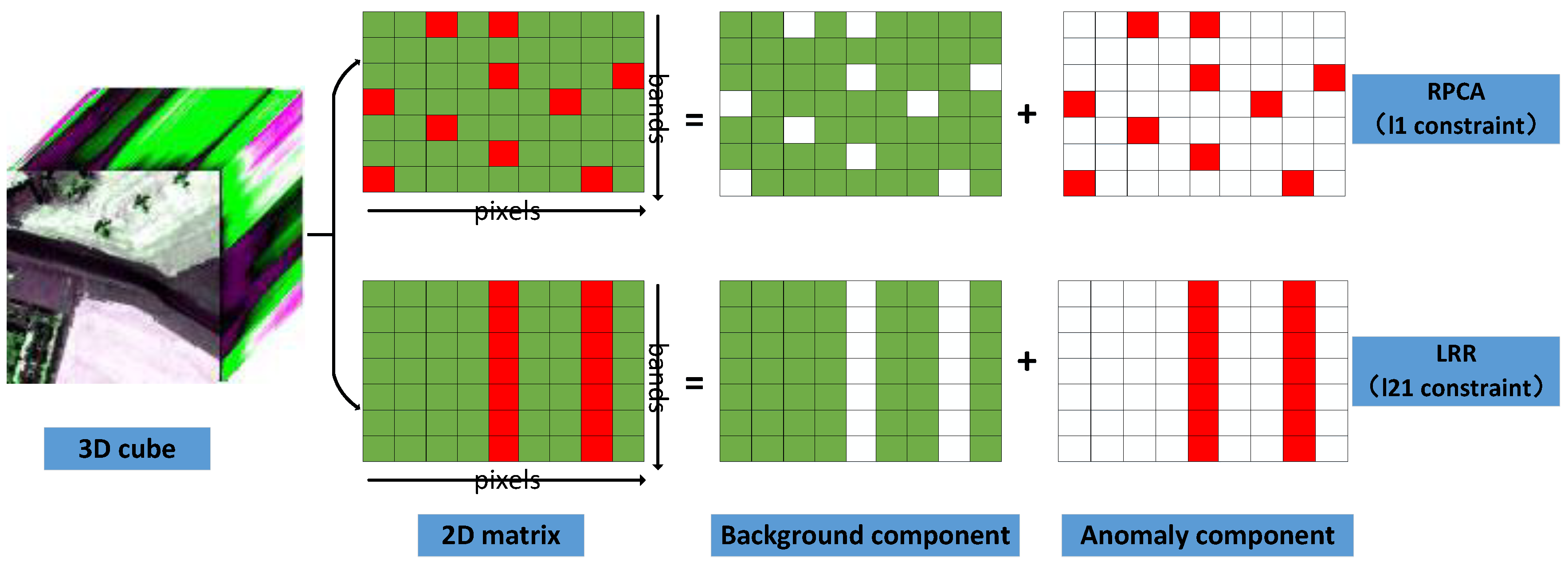
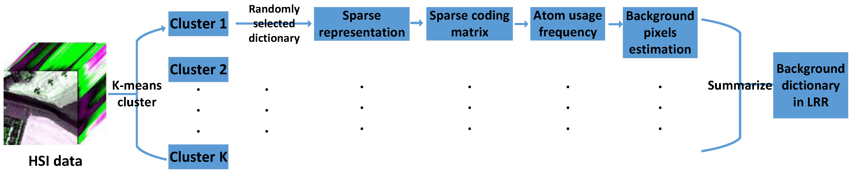
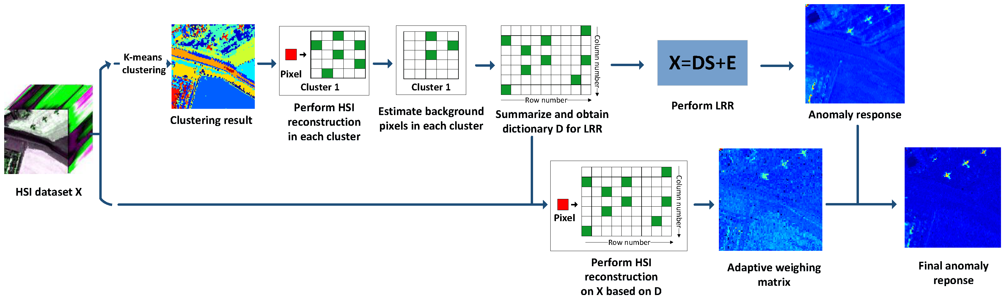
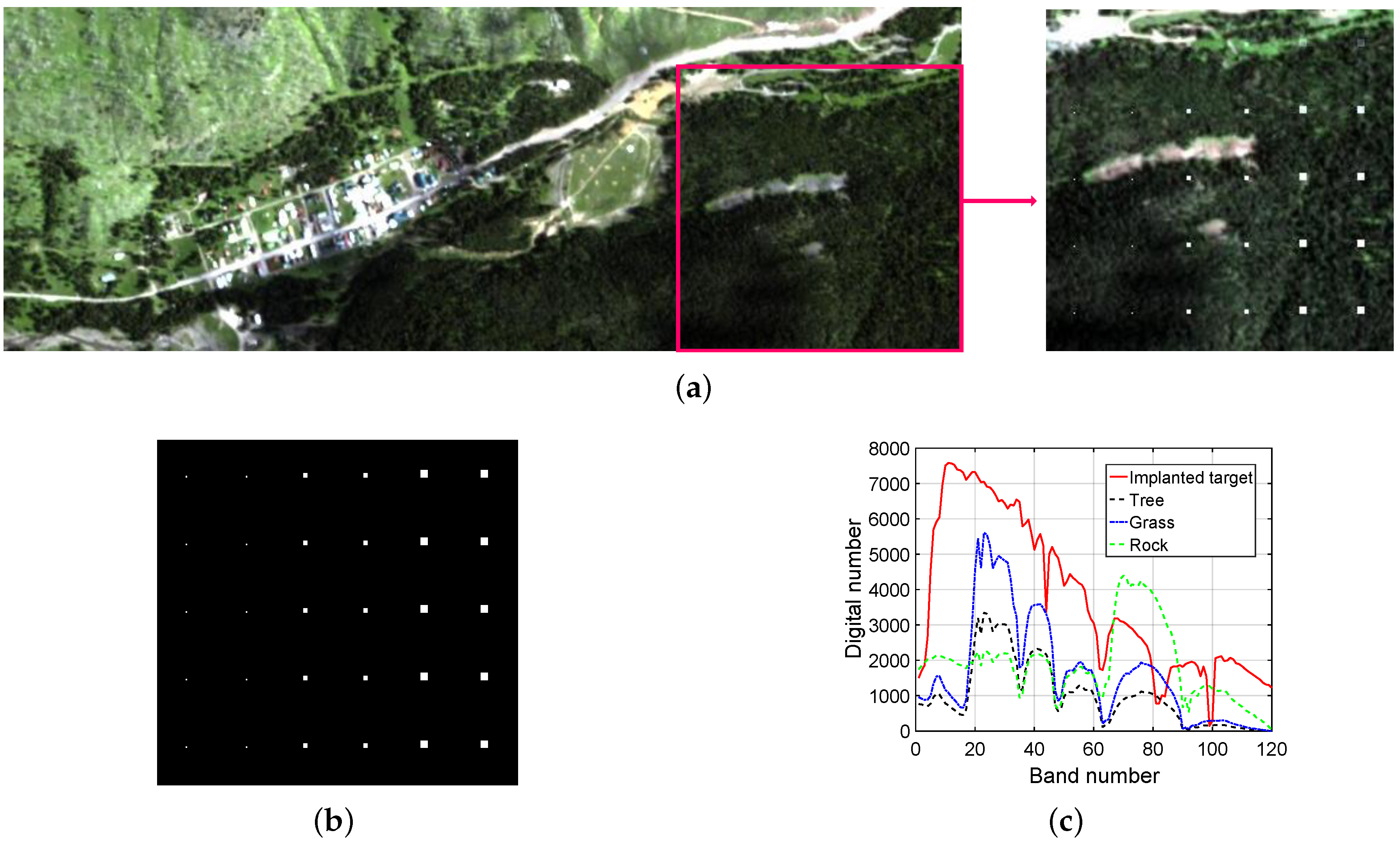
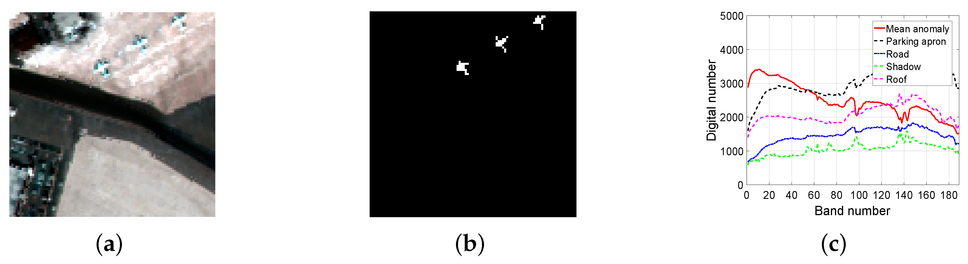
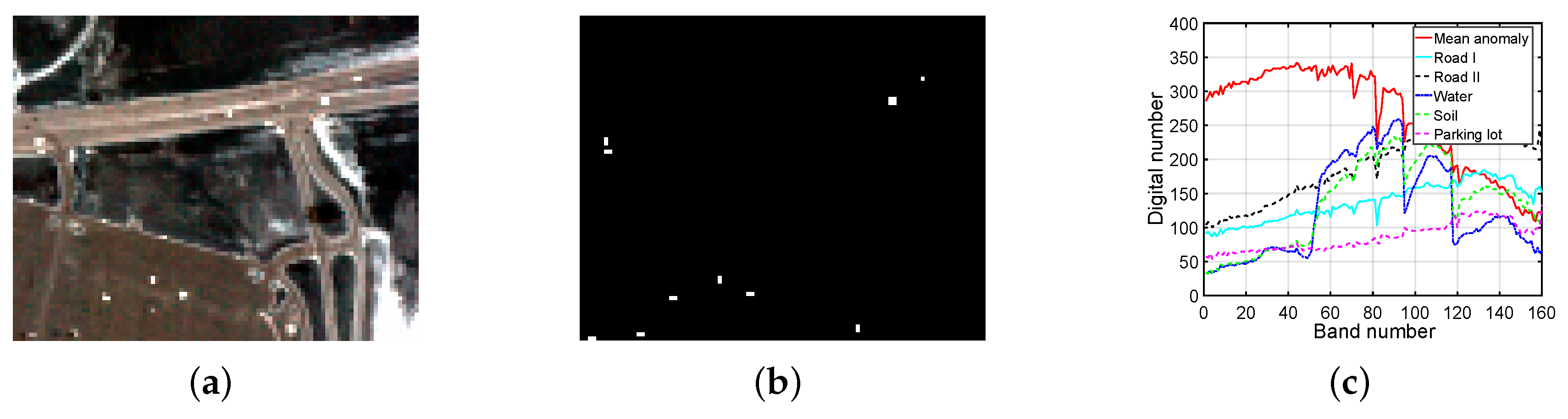
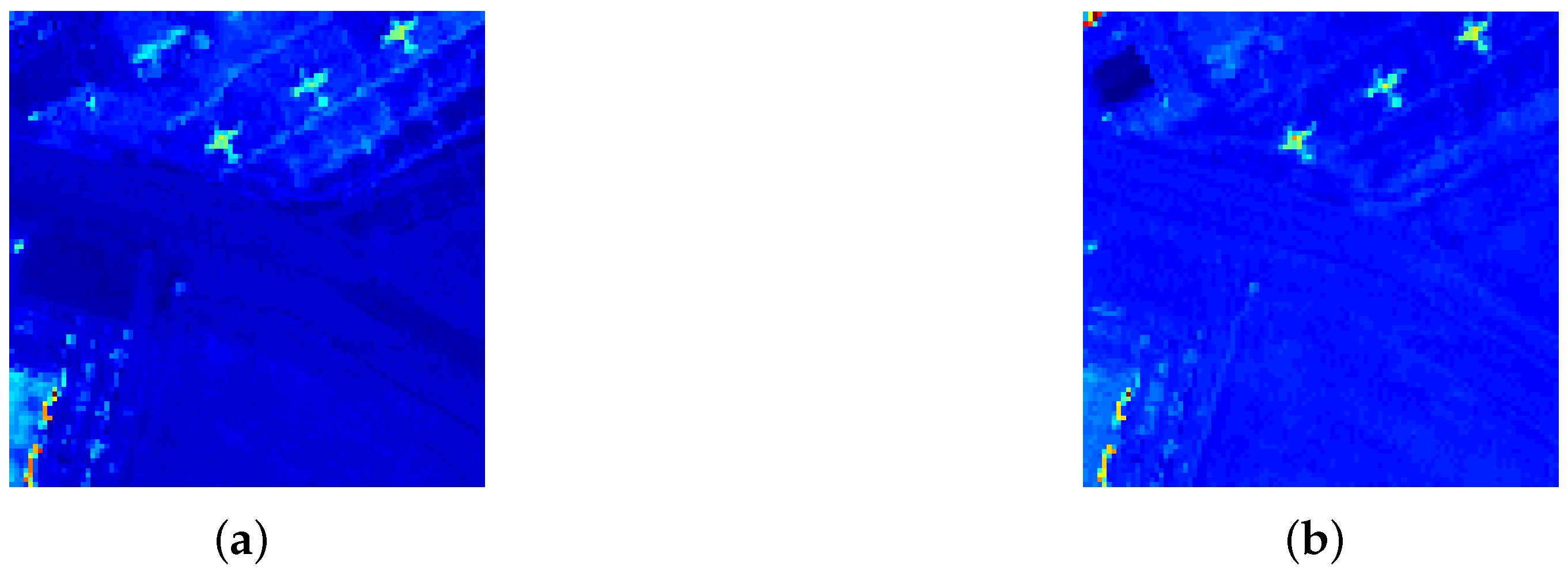
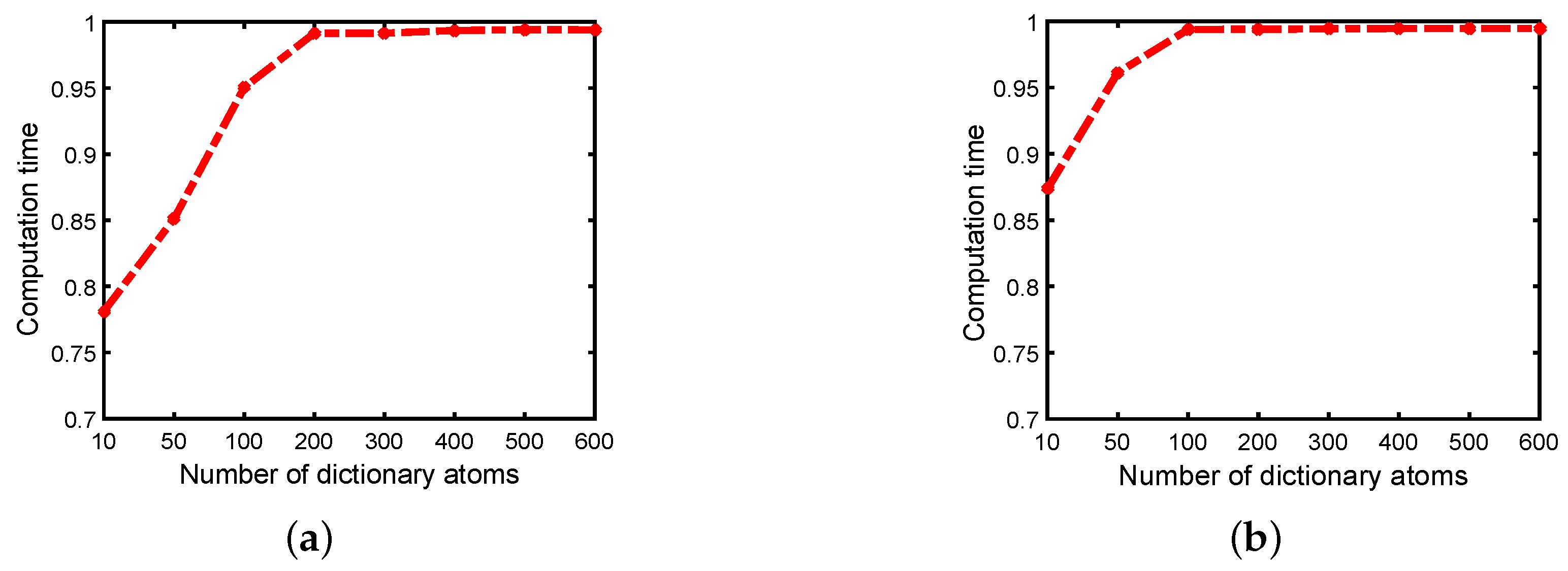
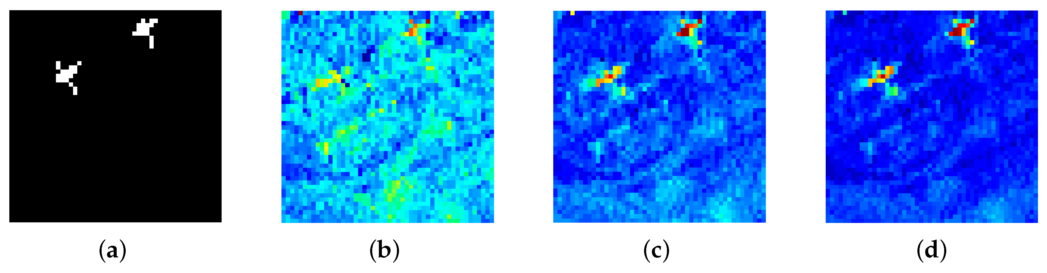
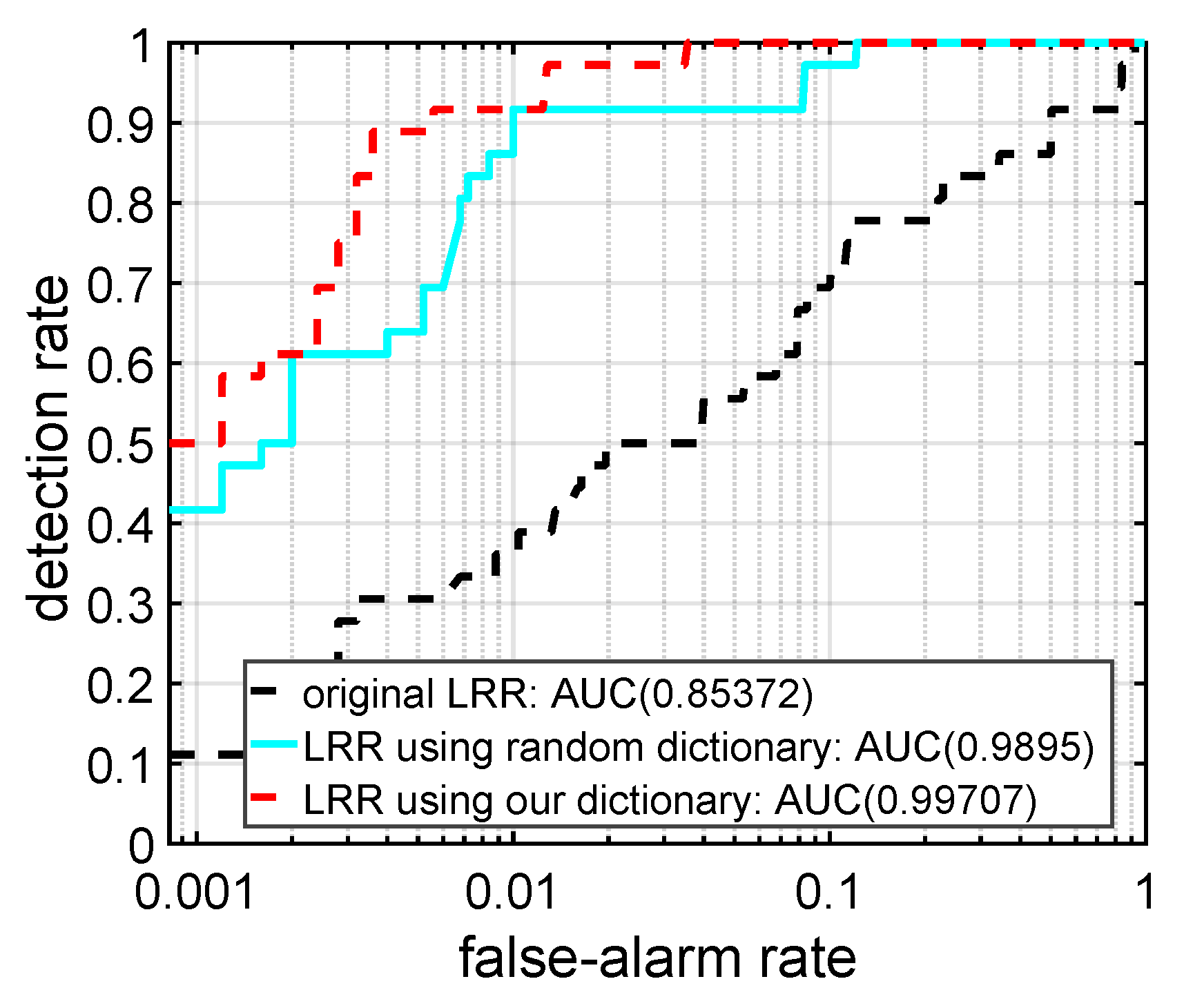
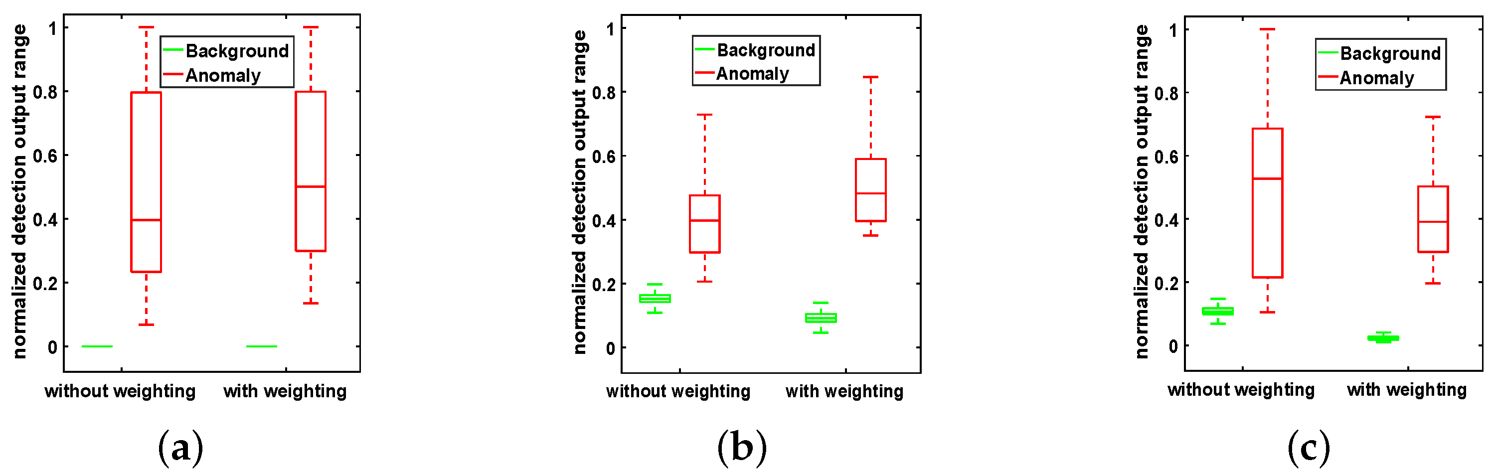
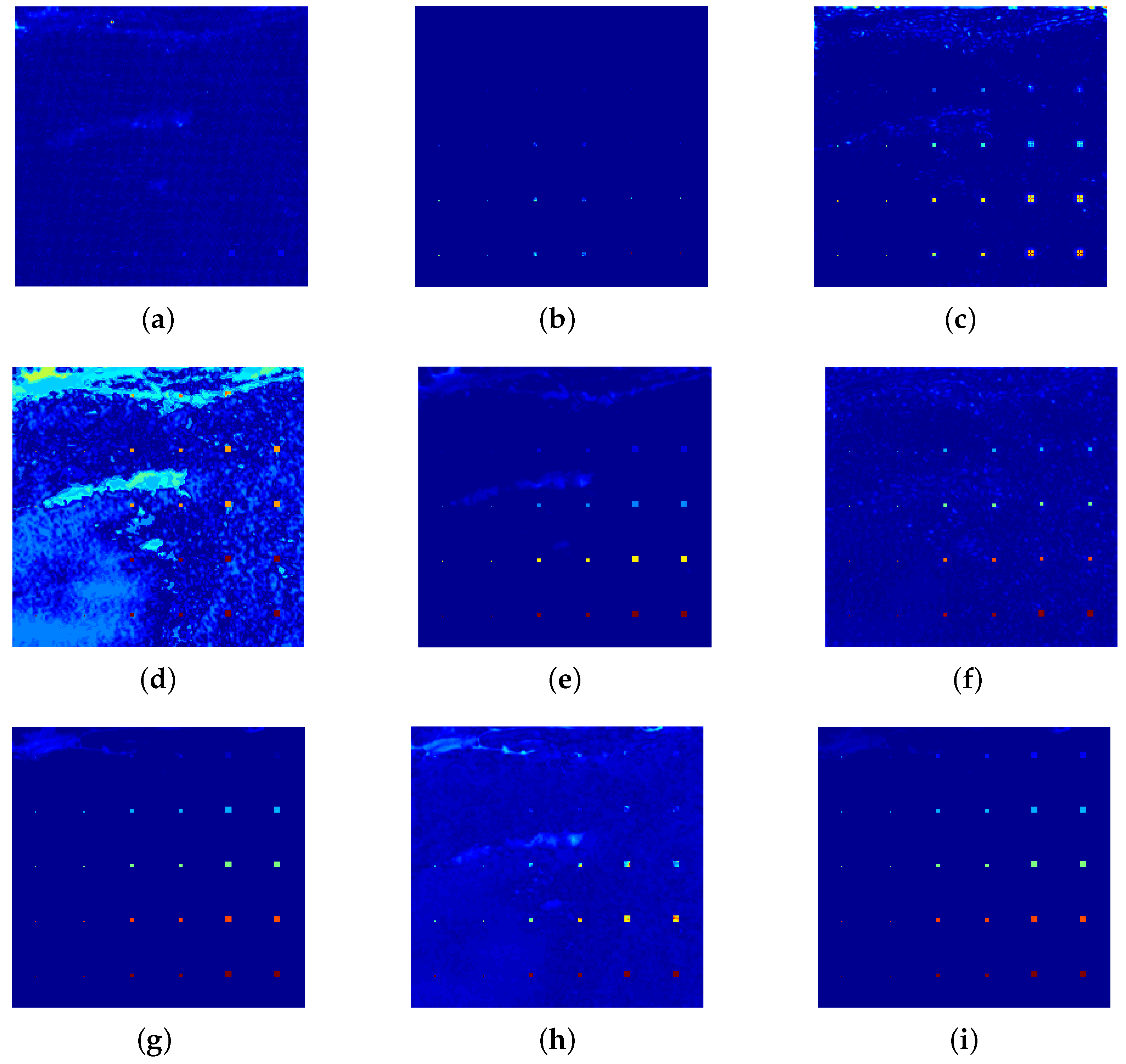
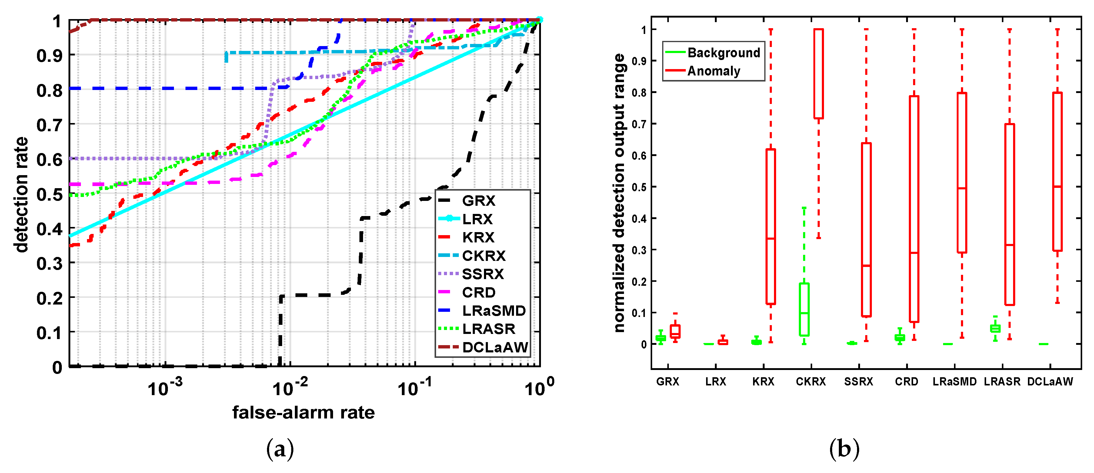
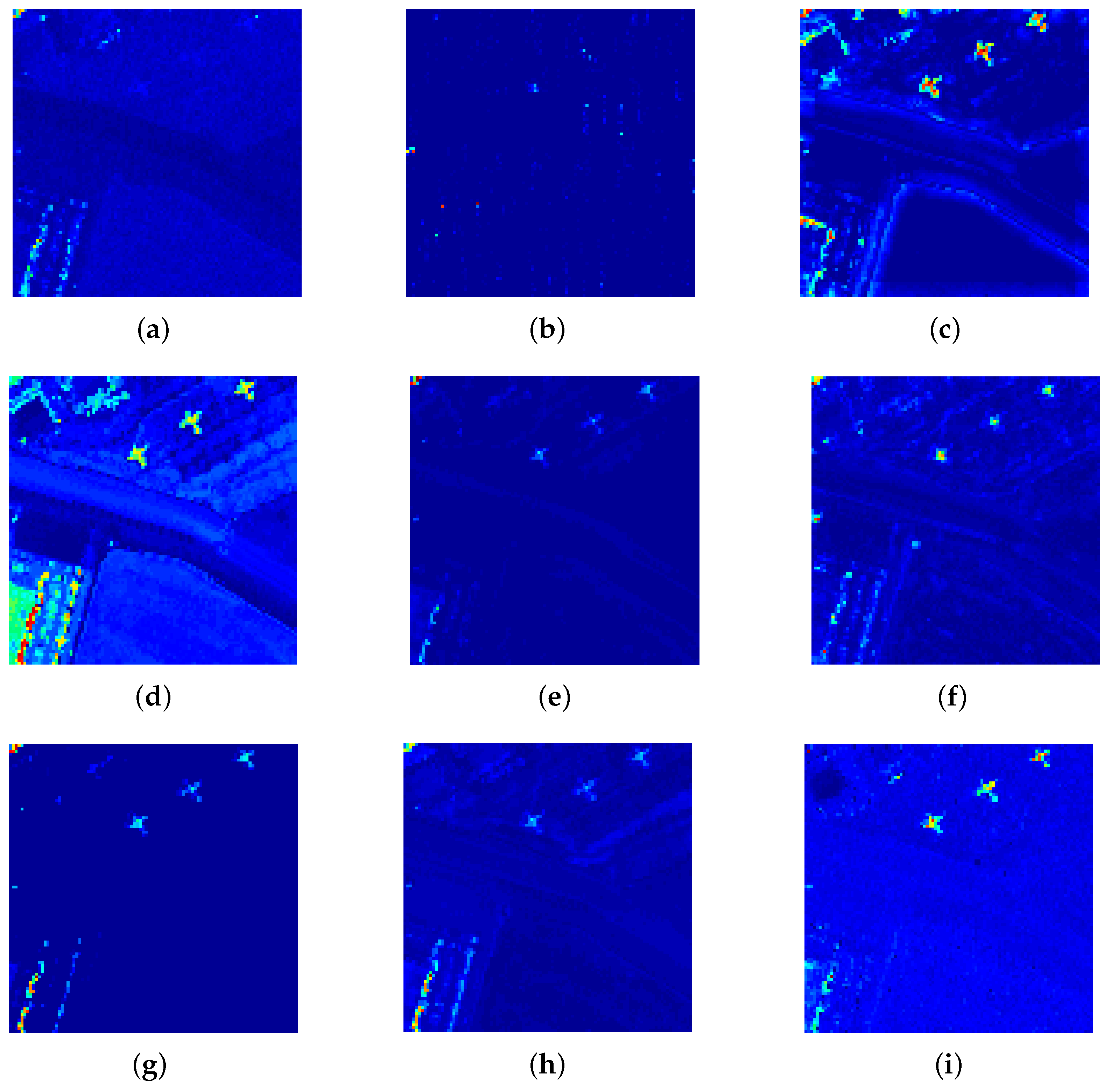
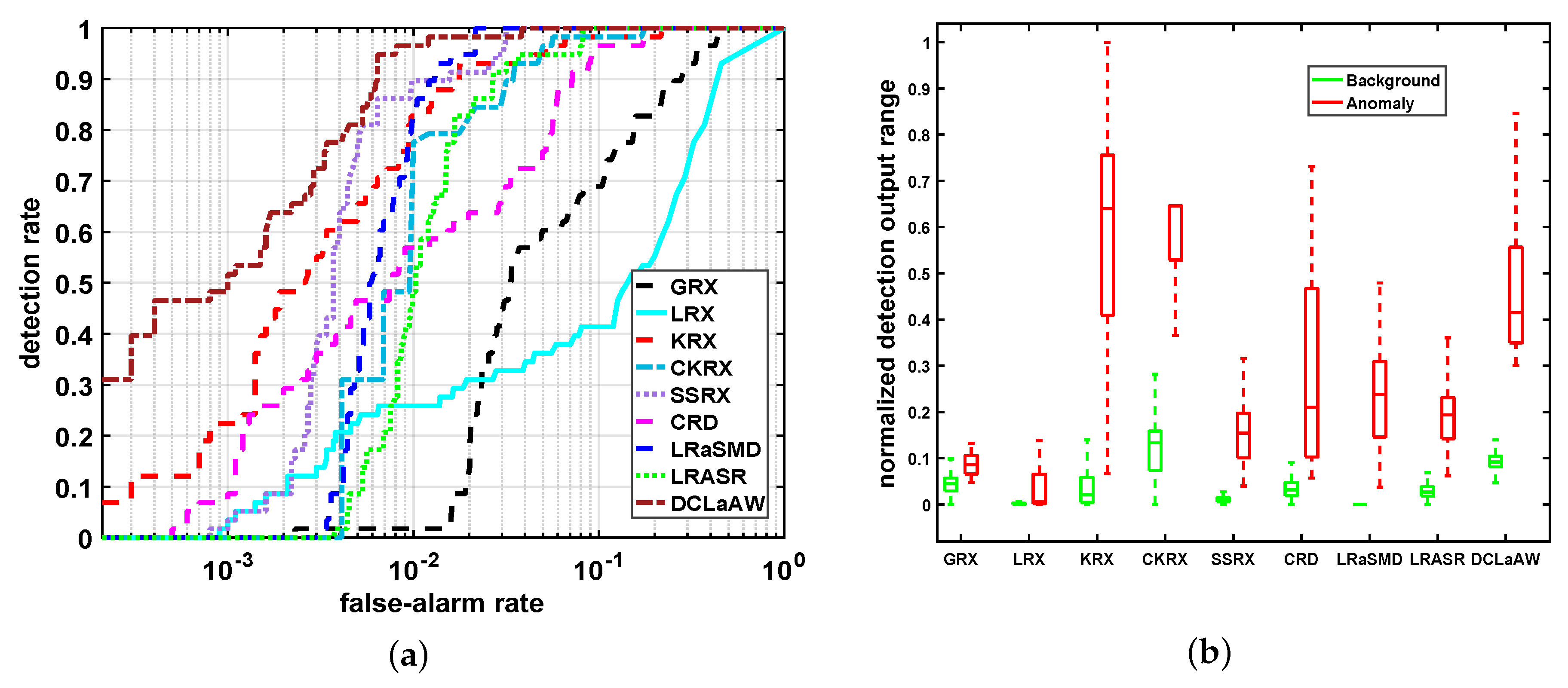
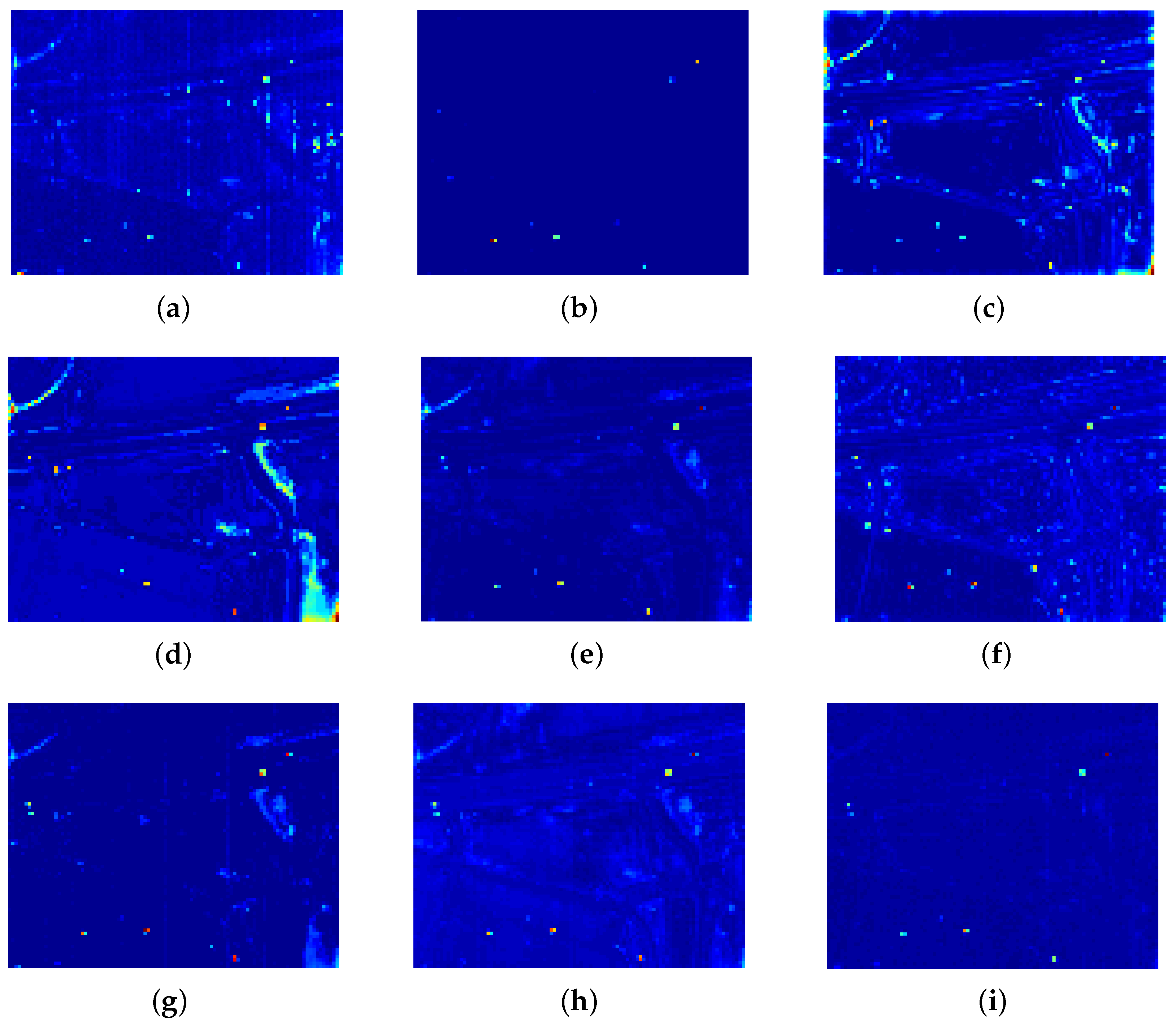
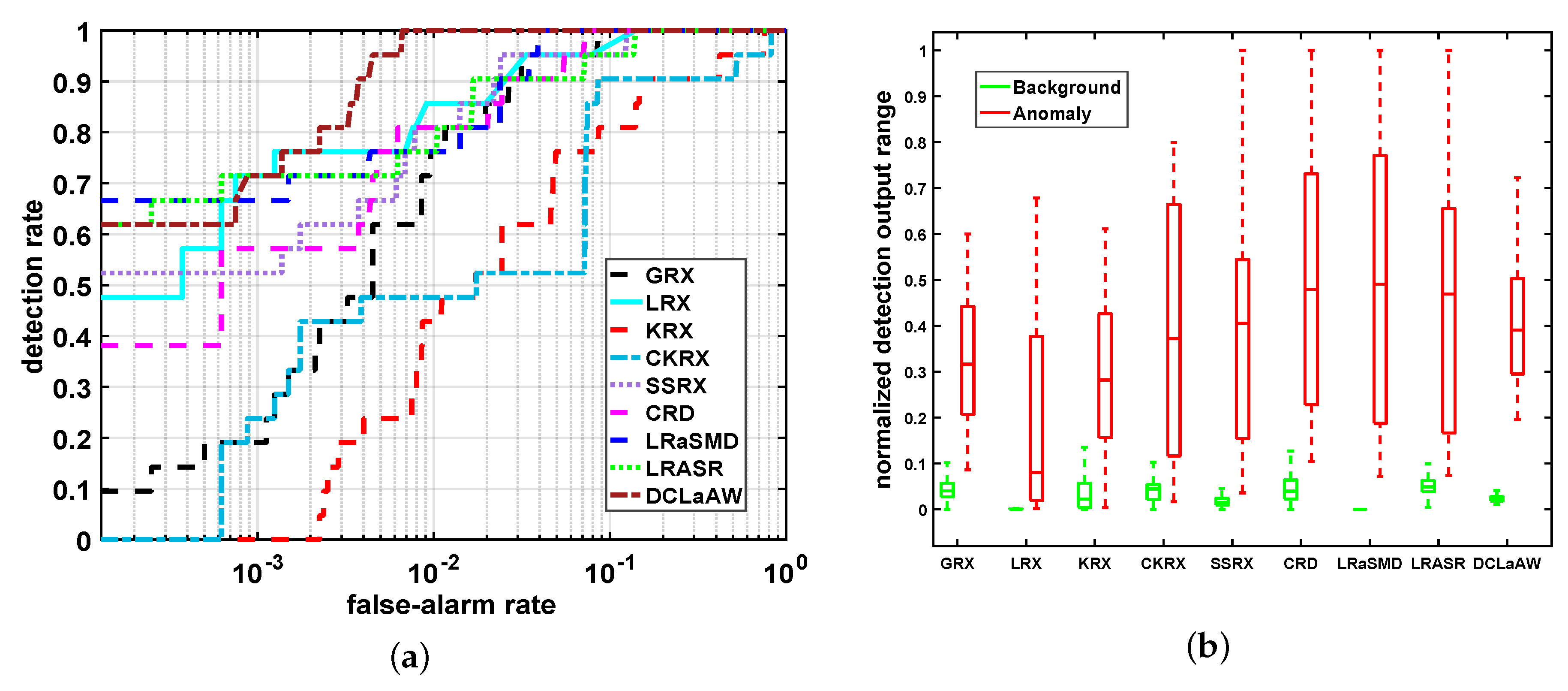
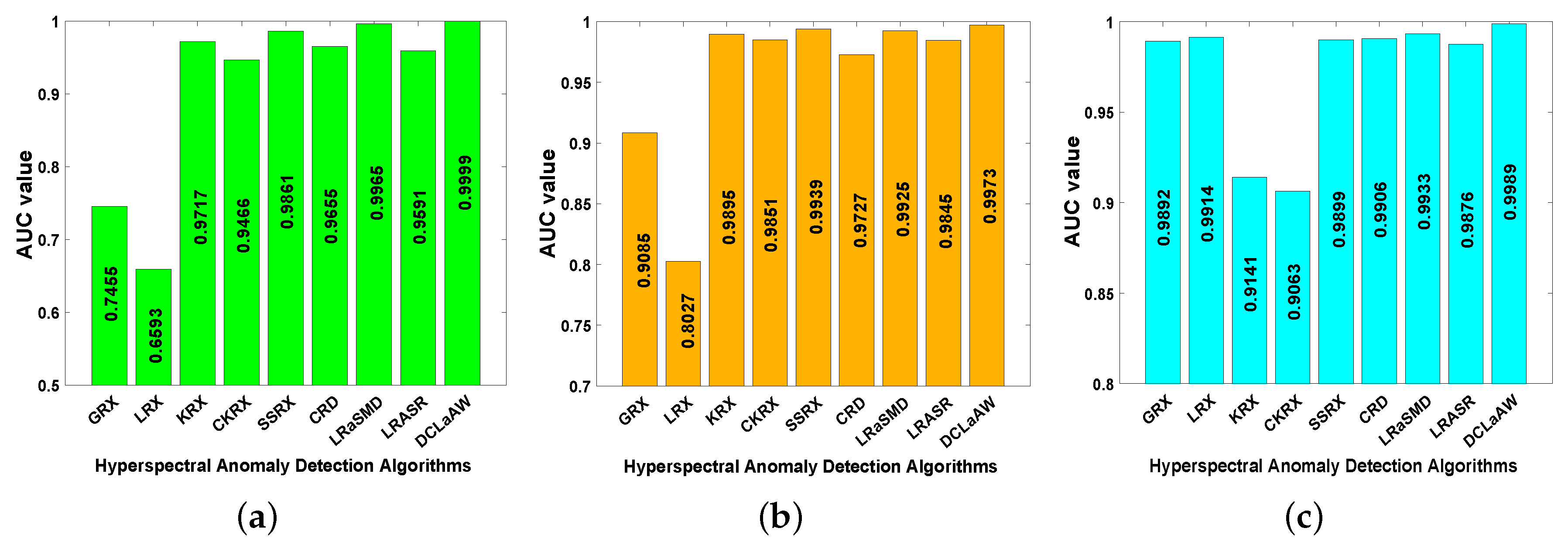
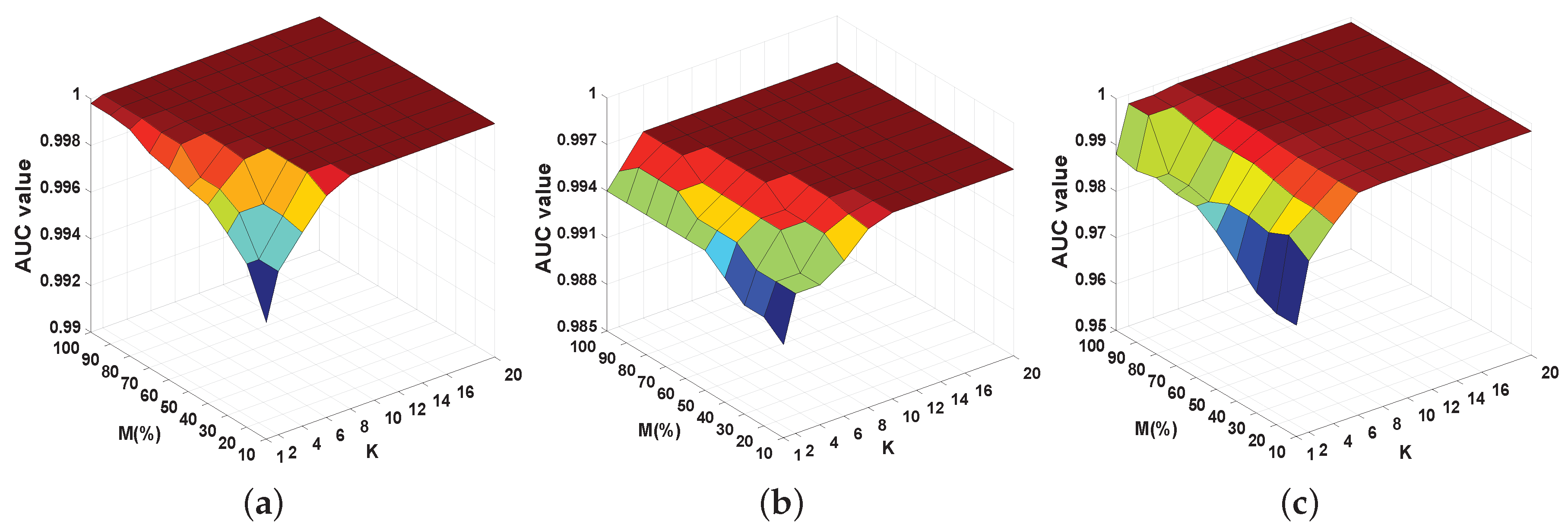
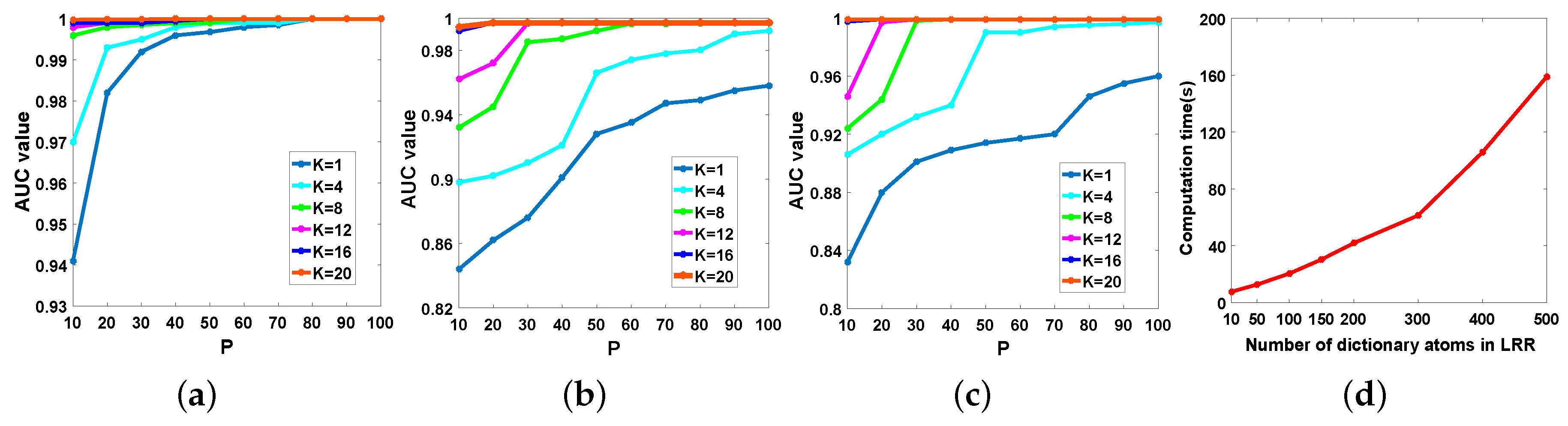
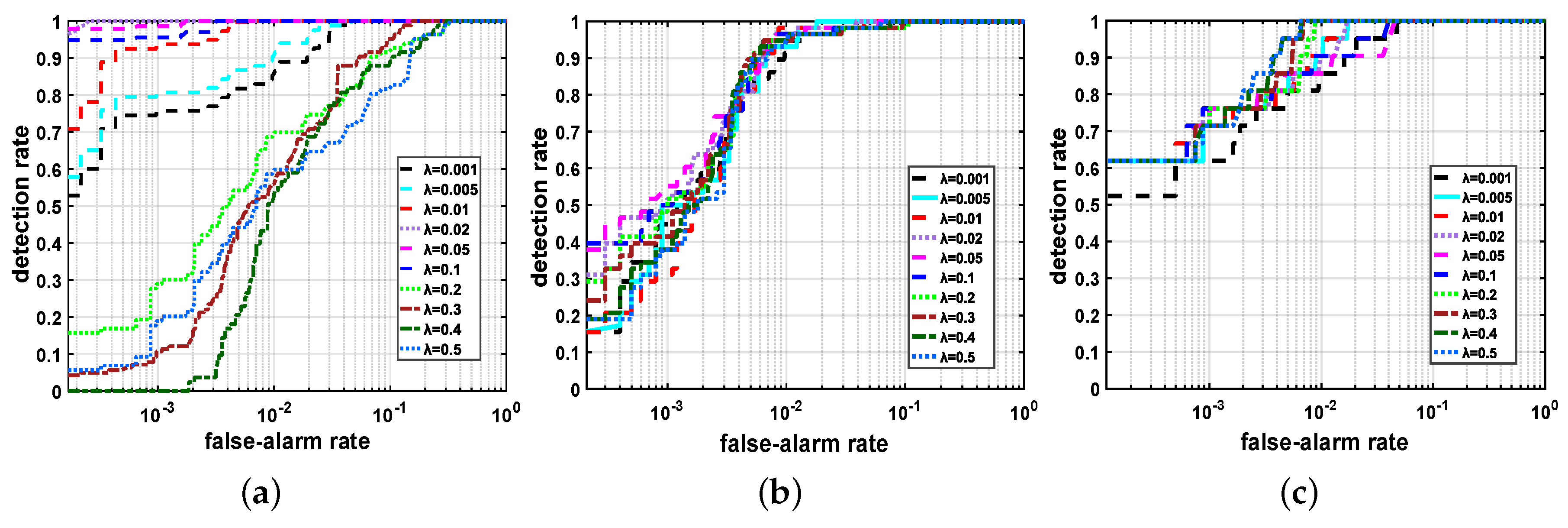
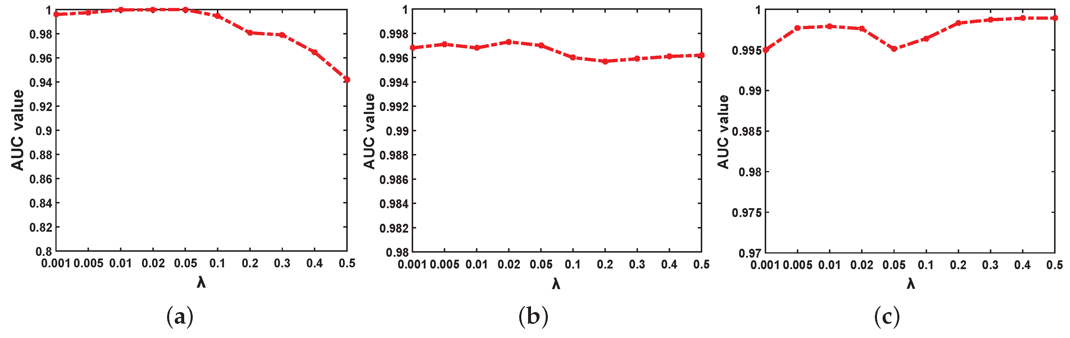
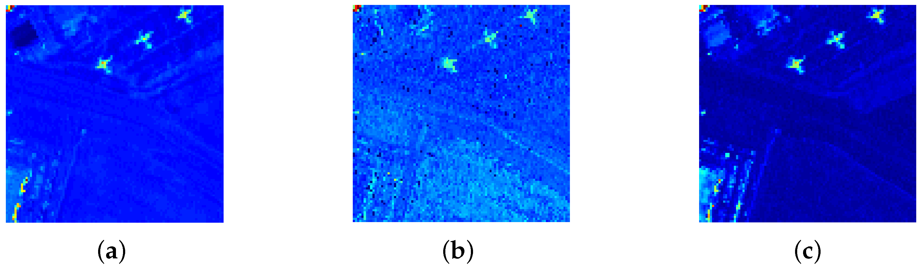
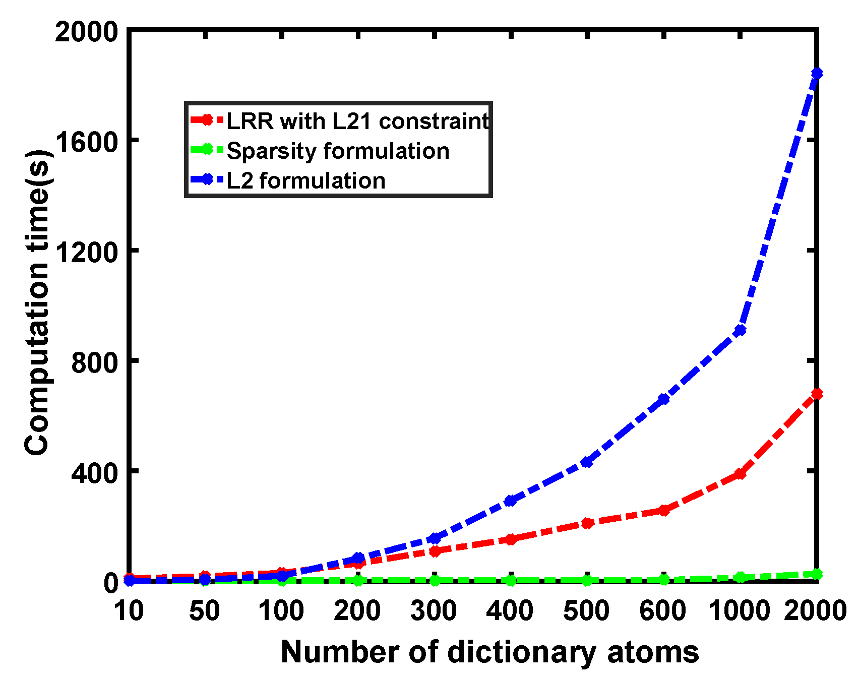
Table 1.
Comparison of models and characteristics of RPCA, LRaSMD and LRR.
| Methods | Models | Theories | Characteristics | |
|---|---|---|---|---|
| RPCA | Abstract the low-rank component as and the sparse component as | Single subspace assumption | l constraint on | |
| LRaSMD | Consider the additional noise; Abstract the low-rank component as and the sparse component as with predefined and | |||
| LRR | Recover the background component using the lowest representation of all data jointly | Multiple subspaces assumption | l constraint on | |
Table 2.
Performance comparison of different constraints for the San Diego dataset.
| Constraint | l Constraint | l Constraint |
|---|---|---|
| AUC value | 0.9936 | 0.9949 |
| Computation time (s) | 72.923 | 49.260 |
Table 3.
Computation times of LRR using different dictionaries for the toy dataset.
| Time(s) | Original LRR | LRR Using Random Dictionary | LRR Using Our Dictionary |
|---|---|---|---|
| Toy Dataset | 1340.505 | 9.471 | 11.057 |
Table 4.
Computational costs of all compared detectors for each dataset.
| Times (s) | GRX | LRX | KRX | CKRX | SSRX | CRD | LRaSMD | LRASR | DCLaAW |
|---|---|---|---|---|---|---|---|---|---|
| Synthetic Dataset | 0.698 | 87.726 | 21.043 | 11.823 | 0.464 | 32.134 | 58.079 | 520.356 | 466.527 |
| San Diego Dataset | 0.157 | 48.108 | 10.218 | 1.946 | 0.161 | 9.953 | 16.885 | 62.877 | 60.015 |
| Urban Dataset | 0.143 | 20.930 | 2.561 | 1.677 | 0.155 | 2.552 | 10.919 | 58.111 | 55.787 |
Table 5.
AUC values obtained by different approaches for the San Diego dataset.
| Approach | LRR with l Constraint | Sparsity Formulation | l Formulation |
|---|---|---|---|
| AUC value | 0.9949 | 0.9922 | 0.9937 |
© 2019 by the authors. Licensee MDPI, Basel, Switzerland. This article is an open access article distributed under the terms and conditions of the Creative Commons Attribution (CC BY) license (http://creativecommons.org/licenses/by/4.0/).
Share and Cite
MDPI and ACS Style
Yang, Y.; Zhang, J.; Song, S.; Liu, D. Hyperspectral Anomaly Detection via Dictionary Construction-Based Low-Rank Representation and Adaptive Weighting. Remote Sens. 2019, 11, 192. https://0-doi-org.brum.beds.ac.uk/10.3390/rs11020192
AMA Style
Yang Y, Zhang J, Song S, Liu D. Hyperspectral Anomaly Detection via Dictionary Construction-Based Low-Rank Representation and Adaptive Weighting. Remote Sensing. 2019; 11(2):192. https://0-doi-org.brum.beds.ac.uk/10.3390/rs11020192
Chicago/Turabian StyleYang, Yixin, Jianqi Zhang, Shangzhen Song, and Delian Liu. 2019. "Hyperspectral Anomaly Detection via Dictionary Construction-Based Low-Rank Representation and Adaptive Weighting" Remote Sensing 11, no. 2: 192. https://0-doi-org.brum.beds.ac.uk/10.3390/rs11020192
Note that from the first issue of 2016, this journal uses article numbers instead of page numbers. See further details here.