Refined Two-Stage Programming Approach of Phase Unwrapping for Multi-Baseline SAR Interferograms Using the Unscented Kalman Filter

Abstract

Phase unwrapping (PU) represents a key step in the reconstruction of digital elevation models (DEMs) and the monitoring of surface deformation from interferometric synthetic aperture radar (InSAR) data. Compared with single-baseline (SB) PU, multi-baseline (MB) PU can resolve the phase discontinuities caused by noise and phase layover induced by terrain undulations. However, the MB PU performance is limited primarily by its poor robustness to measurement bias and noise. To address this problem, we propose a refined 2-D MB PU method based on the two-stage programming approach (TSPA). The proposed method uses the unscented Kalman filter (UKF) to improve the performance of the second stage of the original TSPA method. Specifically, the proposed method maintains the first stage of the TSPA to estimate the range and azimuth gradients between neighbouring pixels. Then, median filtering is slightly used to reduce the effects of the noise gradients on the estimated phase gradients. Finally, the UKF model is used to unwrap the interferometric phases using an efficient quality-guided strategy based on heap-sort. This paper is the first to integrate the UKF into the TSPA framework. The proposed method is validated using bistatic and monostatic MB InSAR datasets, and the experimental results show that the proposed method is effective for MB PU problems.

1. Introduction

Digital elevation models (DEMs) have been widely used in military, civil and economic development. Interferometric synthetic aperture radar (InSAR) constitutes one of the main methods employed for DEM production [1,2,3]. InSAR technology is based on the relationship between the absolute phase and the terrain height, where the absolute phase is obtained by conjugating two SAR images. However, the absolute phase is wrapped in the interval $\left(-\pi ,\pi \right]$; thus, the absolute phase must be unwrapped using a process known as phase unwrapping (PU) before further use. Therefore, PU represents a key step in InSAR data processing that can directly affect the accuracy. Traditional single-baseline (SB) PU is based on the phase continuity assumption, which states that the difference between adjacent pixels cannot exceed $\pi$. Accordingly, the SB PU method can obtain achieves better results in flat terrain and phase continuous regions. However, the phase continuity assumption is not applicable in steep mountains and urban regions; consequently, it is difficult for the traditional SB PU method to obtain good results in discontinuous regions. In contrast, based on the baseline diversity, multi-baseline (MB) PU can combine the information associated with multiple interferograms with different normal baseline lengths, thereby increasing the ambiguity intervals of the absolute phases. Under these conditions, MB PU will be more effective on terrain exhibiting phase layover and phase undersampling issues; as a result, the MB PU method has received increasing attention in recent years.

Several MB PU methods have been proposed over the past couple of decades [4,5,6]. From a pattern recognition perspective, MB PU methods can be roughly divided into two categories [1]. The first category is the parametric phase estimation method represented by maximum likelihood (ML) estimation [4,7,8] and maximum a posteriori (MAP) estimation [9,10,11,12,13]. The ML phase estimation approach first uses the InSAR probability density function to build the likelihood function of the absolute phase, after which a statistical framework is formulated through the ML to estimate the absolute phase. However, the ML method requires a large number of qualified interferograms to obtain the satisfied noise robustness. MAP estimation techniques [9,10,11,12,13] are similar to the ML method insomuch that they estimate the absolute phase based on the probability density function. However, although the MAP technique has a better robustness than the ML approach, the MAP method requires iterative calculations and is thus limited by the computational efficiency and optimization steps. The shortcomings of the ML and MAP methods were analysed in [14,15], and corresponding improved methods were proposed. The second category of MB PU methods consists of nonparametric phase estimation methods, which directly estimate the absolute phase by MB wrapped phase data sets without using the InSAR probability density function. For example, in [16], H. Yu proposed an MB PU method based on cluster analysis (CA) that translates the PU problem into an unsupervised learning problem and then utilizes the CA technique to estimate the absolute phase by establishing a formulation between interferometric phases with different baselines. Afterwards, according to the advantages and disadvantages of the CA method, several improved CA methods were proposed by [17,18]. In addition to the aforementioned MB PU methods, an MB PU method based on the Chinese remainder theorem (CRT) was proposed in [19] that estimates the ambiguity numbers of different baselines by solving the congruence equations. The CRT can accurately obtain the absolute phase when the interferometric phases are free of noise; accordingly, this method is particularly susceptible to noise, and thus, a small amount of measurement bias will result in significant PU errors. Therefore, many methods have been proposed to improve the robustness of the CRT method [20,21,22]. In Ref. [23] Thompson proposed a recursive MB PU method that guides the PU of long-baseline interferometric phases by utilizing short-baseline interferometric phases based on the relationship between the long- and short-baseline interferometric phases. In 2016, Yu and Lan proposed a robust two-dimensional PU method for a two-stage programming approach (TSPA) [1]. This method proposed a novel framework that combines SB PU with MB PU to solve the PU problem. First, the ambiguity numbers were estimated from the interferometric phases of different baselines by the CRT method, after which PU was performed according to the gradients estimated by the SB PU method. By combining SB PU with MB PU, this method improves the robustness of the entire process by improving the robustness of the SB PU method; nevertheless, the robustness and efficiency of this 2-D PU method still needs to be further improved. In summary, because it does not need to obey the phase continuity assumption, MB PU has a wider application scope than SB PU in areas with strong terrain variations. However, the MB PU technique is limited mainly by its noise robustness and efficiency due to the following reasons: (i) its mathematical foundation, i.e., the CRT, is excessively sensitive to measurement biases and thus cannot be applied directly; and (ii) in the MB PU method, multiple interferograms need to be processed simultaneously.

The Kalman filter PU technique is famous for its strong noise robustness in the SB PU domain because it allows PU to be performed simultaneously with noise filtering [24,25,26]. Due to its robust PU accuracy, the unscented Kalman filter (UKF) technique has been widely used in SB PU. In [27], Xie and Pi proposed an MB UKFPU approach that unwraps the interferometric phases of different baselines and then weights the PU results. Consequently, the potential of UKFPU has been thoroughly investigated by some researchers. For example, in [28], Xie proposed a new gradient estimation method that uses a short-baseline PU result to estimate the gradient of the long-baseline interferometric phase and then performs UKFPU on the long-baseline interferometric phase.

In this paper, a refined TSPA method referred to as TSPA-UKFPU is proposed. Using the framework, TSPA-UKFPU transplants the UKF technique into the MB PU domain. The proposed method uses the first stage of the traditional TSPA to estimate the phase gradients. Then, a median filtering algorithm equipped with information characterized by better details is used to filter the range and azimuth gradients slightly, thereby reducing the effect of the noise gradient on the PU results. Finally, the UKF model is used for PU and filtering simultaneously based on an efficient quality-guided strategy. This paper uses two simulated data sets and two real experimental data sets to validate the proposed approach. The results show that the TSPA-UKFPU method exhibits a better noise robustness and a higher efficiency than the traditional TSPA method.

The remainder of this paper is organized as follows. In Section 2, a review of the traditional TSPA PU method is provided. Then, the design of the TSPA-UKFPU method is illustrated in Section 3. In Section 4, the performance of the TSPA-UKFPU method is investigated by experiments with both simulated and real InSAR data sets. In Section 5, the advantages and limitations of the proposed method are further discussed. Finally, the summary and conclusions are provided in Section 6.

2. Review of the TSPA

2.1. Mathematical Foundation of MB PU

MB PU can resolve the phase discontinuity issues caused by phase layover and phase undersampling using the baseline diversity. In other words, the MB PU technique is particularly applicable to regions with terrain exhibiting steep fluctuations. The wrapped interferometric phase is obtained by conjugating two SAR images [29,30] with the following:

$$\mathsf{\Phi }(k)=a(k)\exp (j\cdot \phi (k))$$

(1)

where $\mathsf{\Phi }(k)$ is the complex interferometric measurement after conjugation multiplication of the $k$th pixel, $a(k)$ is the interferometric amplitude of the $k$th pixel, and $\phi (k)$ is the wrapped interferometric phase of the $k$th pixel. The measured wrapped interferometric phase has the following relationship with the absolute phase:

$$\phi (k)=\psi (k)-2n(k)\pi$$

(2)

where $\psi (k)$ is the absolute phase of the $k$th pixel. According to Equation (2), the purpose of PU is to determine the absolute phase from the wrapped phase. If the interferometric phase is free of noise, then the absolute phase $\psi (k)$ can be obtained by finding the ambiguity number $n(k)$. Based on the InSAR geometry, the terrain height can be calculated from the absolute phase:

$$h(k)=\frac{\lambda \cdot r(k)\cdot \sin (\theta )}{B\cdot 4\pi }\cdot \psi (k)$$

(3)

where $h(k)$ is the terrain height of the $k$th pixel, $\lambda$ is the wavelength, $r(k)$ is the slant range of the target from the master channel of the $k$th pixel, $\theta$ is the incidence angle, and $B$ is the normal baseline (i.e., the perpendicular baseline). Because the terrain height of the corresponding pixel is the same, taking the dual-baseline case as an example, we can combine the absolute phases of two interferograms with different baseline lengths that can be expressed as follows:

$$B_2\cdot ({\phi }_1(k)+2n_1(k)\pi )=B_1\cdot ({\phi }_2(k)+2n_2(k)\pi ) (flattened)$$

(4)

where $B_i(i=1,2)$ represents the baseline length of interferogram $i$, $n_i(k)(i=1,2)$ is the ambiguity number of the $k$th pixel in interferogram $i$, and ${\varphi }_i(k)(i=1,2)$ is the wrapped interferometric phase of the $k$th pixel in interferogram $i$. The term “flattened” means that the flat-earth phases of $n_1(k)$ and $n_2(k)$ have been compensated in Equation (4); these flat-earth terms, which are integers, constitute the two unknowns in Equation (4). Theoretically, we cannot solve $n_1(k)$ and $n_2(k)$ simultaneously using only Equation (4) (as two unknowns cannot be solved with one equation). However, because both $n_1(k)$ and $n_2(k)$ are integers, we know from the CRT that some special combinations of $B_i(i=1,2)$ enable us to solve $n_1(k)$ and $n_2(k)$ using only Equation (4).

2.2. TSPA

Since Equation (4) uses the information of only one pixel (i.e., the $k$th pixel) to obtain the absolute phase, Equation (4) contains excessive measurement bias and thus cannot be used in practice [1]. To address this issue, the TSPA uses the information of all the pixels in an interferogram. If we pick a neighbouring pixel $k-1$ of pixel $k$, according to Equation (4), we will have:

$$B_2\cdot ({\phi }_1(k-1)+2n_1(k-1)\pi )=B_1\cdot ({\phi }_2(k-1)+2n_2(k-1)\pi )$$

(5)

By subtracting Equation (5) from Equation (4), we can obtain:

$$B_2\cdot ({\phi }_1(k)-{\phi }_1(k-1)+2(n_1(k)-n_1(k-1))\pi )=B_1\cdot ({\phi }_2(k)-{\phi }_2(k-1)+2(n_2(k)-n_2(k-1))\pi )$$

(6)

If we allow $n_1(k)-n_1(k-1)=\widehat{\Delta }{n}_1(k,k-1)$ and $n_2(k)-n_2(k-1)=\widehat{\Delta }{n}_2(k,k-1)$, Equation (6) can be further rewritten as:

$$B_2\cdot ({\phi }_1(k)-{\phi }_1(k-1)+2(\widehat{\Delta }{n}_1(k,k-1))\pi )=B_1\cdot ({\phi }_2(k)-{\phi }_2(k-1)+2(\widehat{\Delta }{n}_2(k,k-1))\pi )$$

(7)

In Equation (7), only $\widehat{\Delta }{n}_1(k,k-1)$ and $\widehat{\Delta }{n}_2(k,k-1)$ are unknown, and they can be considered as the gradient information between neighbouring pixels. Moreover, $\widehat{\Delta }{n}_1(k,k-1)$ and $\widehat{\Delta }{n}_2(k,k-1)$ are integers; therefore, we can use the CRT to solve Equation (7) as well (Equations (4) and (7) share the same mathematical conditions). If we allow $R(\widehat{\Delta }{n}_1(k,k-1),$$\widehat{\Delta }{n}_2(k,k-1))=B_2\cdot (({\phi }_1(k)-{\phi }_1(k-1))+2(\widehat{\Delta }{n}_1(k,k-1))\pi )-B_1\cdot (({\phi }_2(k)-{\phi }_2(k-1))+2(\widehat{\Delta }{n}_2(k,k-1))\pi )$, the gradient of the ambiguity numbers $\widehat{\Delta }{n}_1(k,k-1)$ and $\widehat{\Delta }{n}_2(k,k-1)$ can be obtained by the CRT-based optimization model:

$$\arg \underset{\begin{array}{l}\widehat{\Delta }{n}_1(k,k-1)\\ \widehat{\Delta }{n}_2(k,k-1)\end{array}}{\min }\left|R(\widehat{\Delta }{n}_1(k,k-1),\widehat{\Delta }{n}_2(k,k-1))\right|, \widehat{\Delta }{n}_1(k,k-1),\widehat{\Delta }{n}_2(k,k-1)\in \mathrm{integer}$$

(8)

Step 2 of the TSPA is an SB PU framework. According to [1], the traditional TSPA adopts the SB $L^1$-norm PU method:

$$\arg \underset{n_i(k)}{\min }{\displaystyle \sum _{(k,k-1)}\left|n_i(k)-n_i(k-1)-\widehat{\Delta }{n}_i(k,k-1)\right|}$$

(9)

where $\widehat{\Delta }{n}_i(k,k-1)$ is the estimated absolute phase difference between pixel $k$ and pixel $k-1$, and Equation (9) is the SB $L^1$-norm PU model.

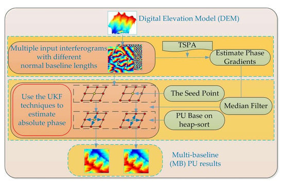
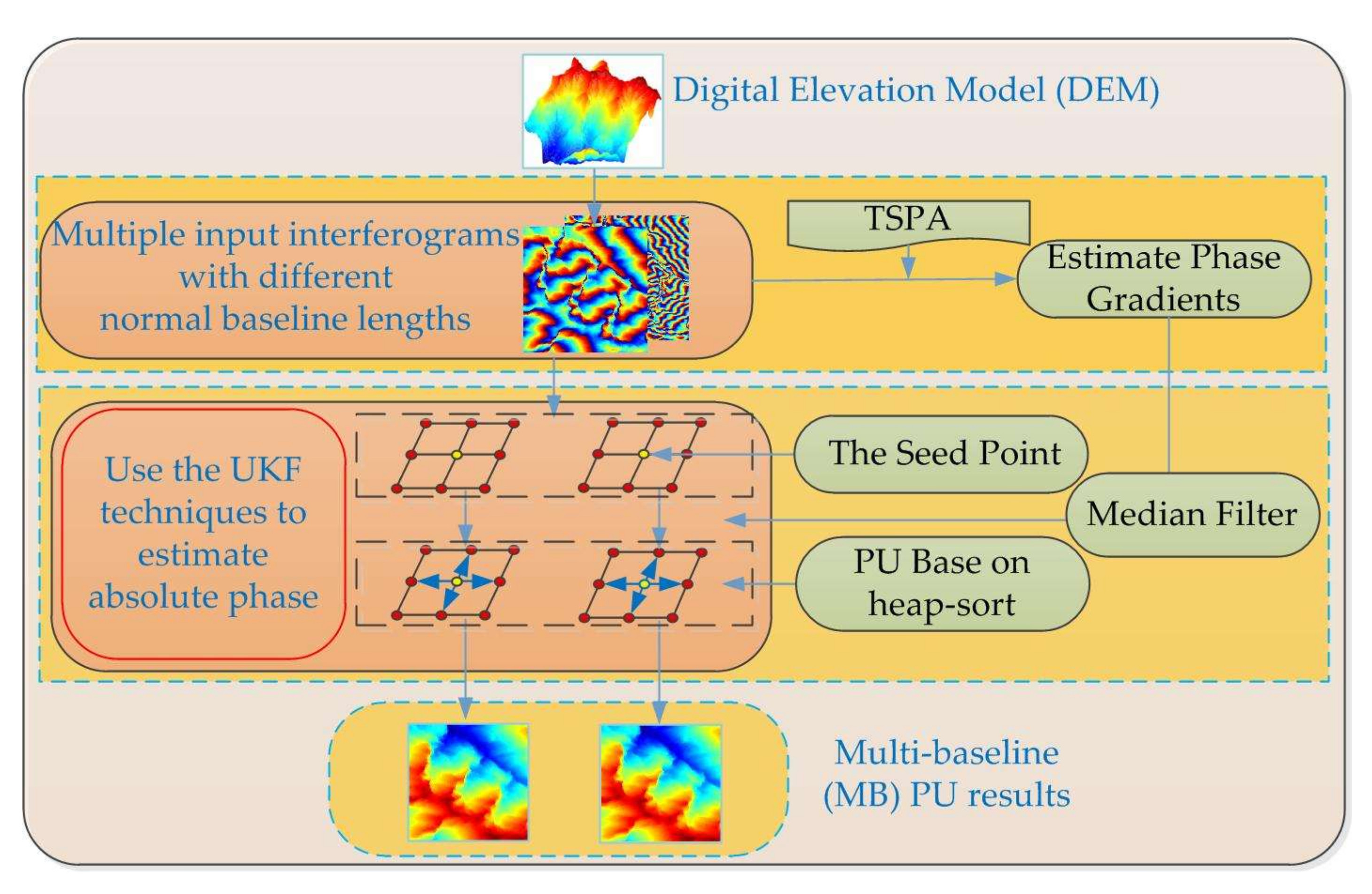
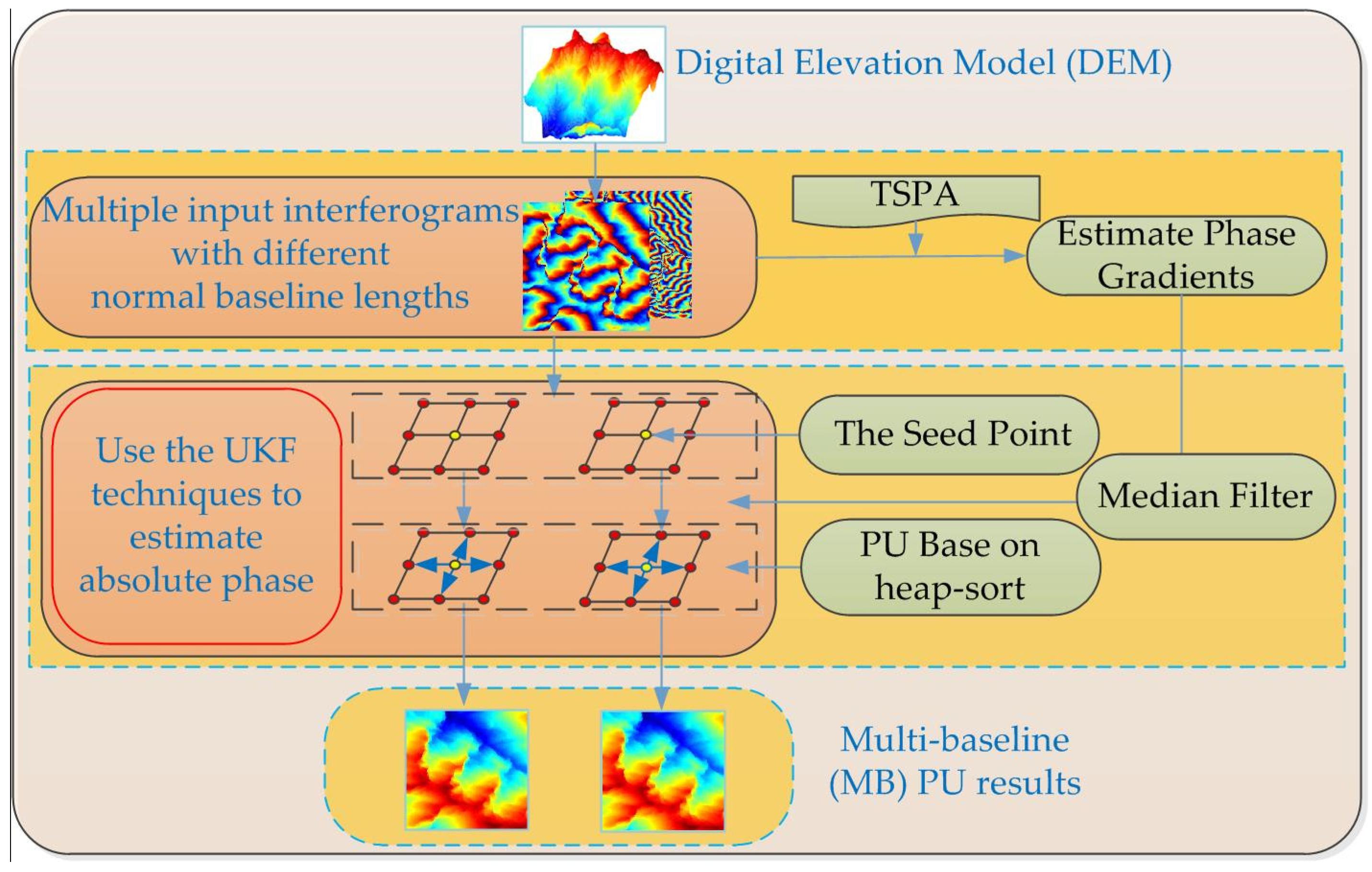
3. TSPA-UKFPU Method

The traditional TSPA PU method can be divided into two steps: (1) estimating the gradient information of the ambiguity number and (2) unwrapping the phase using the SB $L^1$-norm PU model. From Figure 1c,d, we can see that the gradients obtained by the SB PU method are limited to the interval $\left(-\pi ,\pi \right]$. From Figure 1e,f, the gradients obtained by the TSPA are evidently not limited to the interval $\left(-\pi ,\pi \right]$. However, as described above, the CRT possesses remarkably poor noise robustness and thus cannot be used in practice directly. Hence, although stage 1 of the TSPA does not need to obey the phase continuity assumption, the obtained gradient information could be very noisy (as shown in Figure 1e,f). Under this condition, a PU methodology with an extra adaptive filtering function would be preferred in stage 2. UKFPU is representative of one such filtering-based SB PU method. The residuals are the key problem of PU. However, the residuals can be considered as noise in the interferograms. UKFPU is unwrapped based on the gradient estimation variance and the observed variance of the pixels. Moreover, the result of the pixel to be unwrapped is obtained by weighting the unwrapped pixel points among the eight pixels around it. These result in the UKFPU model having better noise robustness. Therefore, UKFPU cannot only suppress the effect of residuals on the PU results, but also filter out the residuals. Accordingly, in the following sections, we will refine the SB UKFPU model and transplant it into stage 2 of the TSPA framework.

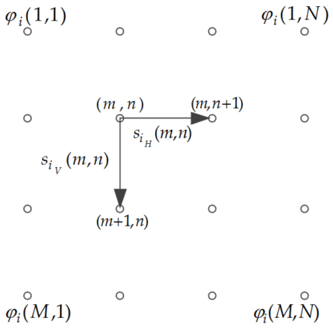
3.1. Estimating the Phase Gradient

Estimating the phase gradient constitutes one of the key steps in both SB PU and MB PU. However, under the SB situation, almost all PU methods adopt the phase continuity assumption, which limits the range of the phase gradient. The gradient information can be obtained by:

$${\widehat{\Delta }}_{\psi }(k,k-1)=\{\begin{array}{ll}\phi (k)-\phi (k-1)& \left|\phi (k)-\phi (k-1) \right|\le \pi \\ \phi (k)-\phi (k-1)-2\pi & \phi (k)-\phi (k-1)>\pi \\ \phi (k)-\phi (k-1)+2\pi & \phi (k)-\phi (k-1)<-\pi \end{array}$$

(10)

where ${\widehat{\Delta }}_{\psi }(k,k-1)$ is the estimated absolute phase difference between pixel $k$ and pixel $k-1$. The indexes $k$ and $k-1$ are general descriptions of the relationships between neighbouring pixels. There are two directions, i.e., horizontal and vertical, for neighbouring pixels. Unfortunately, the noise and absolute phase frequently fail to observe the phase continuity assumption in practice. In this paper, we use the result from stage 1 of the TSPA to estimate the gradient, where the phase continuity assumption does not need to be obeyed. The gradient estimation method is as follows:

Figure 2 shows an interferometric phase with $M\times N$ pixels. According to Equation (2), we can estimate the wrapped range and azimuth gradients. In Figure 2, the coordinates of a pixel are $(m,n)$. According to the relationship between a point and its neighbours, we can obtain the range and azimuth gradients of the pixel as follows:

$$\begin{array}{c}\{\begin{array}{c}{s}_{i_V}={\phi }_i(m+1,n)-{\phi }_i(m,n)\\ s_{i_H}={\phi }_i(m,n+1)-{\phi }_i(m,n)\end{array}\\ (m,n)\in (M,N)\end{array}$$

(11)

where ${\varphi }_i(m,n)$ is the wrapped value of pixel $(m,n)$ in interferogram $i$, and $s_{i_V}$ and $s_{i_H}$ are the range and azimuth wrapped phase gradients, respectively, of ${\varphi }_i(m,n)$. Equation (11) can calculate the range and azimuth wrapped phase gradients of an interferogram. Similarly, the absolute phase gradient can be expressed as:

$$\begin{array}{c}\{\begin{array}{c}{\delta }_{i_V}={\psi }_i(m+1,n)-{\psi }_i(m,n)\\ {\delta }_{i_H}={\psi }_i(m,n+1)-{\psi }_i(m,n)\end{array}\\ (m,n)\in (M,N)\end{array}$$

(12)

where ${\psi }_i(m,n)$ is the absolute phase value of pixel $(m,n)$ in interferogram $i$, and ${\delta }_{i_V}$ and ${\delta }_{i_H}$ are the range and azimuth absolute phase gradients, respectively, of ${\psi }_i(m,n)$. Step 1 of the traditional TSPA method can estimate the ambiguity numbers of these gradients. The ambiguity numbers $\widehat{\Delta }{n}_i(k,k-1)$ can be calculated in Equation (8). Therefore, according to Equations (2), (8), (11), and (12), we can obtain the estimated gradients when the phase is discontinuous as follows:

$$\{\begin{array}{l}\begin{array}{ll}\overline{{\delta }_{i_V}}& ={\psi }_i(m+1,n)-{\psi }_i(m,n)={\phi }_i(m+1,n)-{\phi }_i(m,n)+2\cdot \pi \cdot \widehat{\Delta }{n}_{i_V}\\ & =s_{i_V}+2\cdot \pi \cdot \widehat{\Delta }{n}_{i_V}\\ & ={\overline{s}}_{i_V}+2\cdot \pi \cdot \overline{\Delta }{n}_{i_V}+{\omega }_{i_V}\end{array}\\ \begin{array}{ll}\overline{{\delta }_{i_H}}& ={\psi }_i(m,n+1)-{\psi }_i(m,n)={\phi }_i(m,n+1)-{\phi }_i(m,n)+2\cdot \pi \cdot \widehat{\Delta }{n}_{i_H}\\ & =s_{i_H}+2\cdot \pi \cdot \widehat{\Delta }{n}_{i_H}\\ & ={\overline{s}}_{i_H}+2\cdot \pi \cdot \overline{\Delta }{n}_{i_H}+{\omega }_{i_H}\end{array}\end{array}$$

(13)

where $\overline{{\delta }_{i_V}}$ and $\overline{{\delta }_{i_H}}$ are the medians of all the range and azimuth gradient elements, respectively, in the window centred on $(m,n)$ in interferogram $i$, $\widehat{\Delta }{n}_{i_V}$ and $\widehat{\Delta }{n}_{i_H}$ are the range and azimuth gradient ambiguity numbers, respectively, obtained according to Equation (8), ${\overline{s}}_{i_V}$ and ${\overline{s}}_{i_H}$ are the noise-free wrapped gradients of the range and azimuth, respectively, of pixel $(m,n)$ in interferogram $i$, $\overline{\Delta }{n}_{i_V}$ and $\overline{\Delta }{n}_{i_H}$ are the noise-free range and azimuth gradient ambiguity numbers, respectively, of pixel $(m,n)$ in interferogram $i$, and ${\omega }_{i_V}$ and ${\omega }_{i_H}$ are the range and azimuth gradient estimation errors, respectively, of pixel $(m,n)$ in interferogram $i$. Equation (13) demonstrates that the gradients estimated in this paper are free from the limitation of the phase continuity assumption; that is, the estimated gradients can be greater than $\pi$ or less than $-\pi$.

3.2. UKFPU Algorithm

UKFPU can perform PU and filtering simultaneously, thereby obtaining a dynamic linear state equation based on the relationships between adjacent pixels. The observation equation obtains the characteristics of the complex interferometric phase from the data. The UKF unwraps the pixels one by one; to facilitate this process, the PU component of the UKFPU algorithm is illustrated as a one-dimensional model. Thus, we can obtain the following:

$$\{\begin{array}{l}\begin{array}{ll}{\psi }_i(k)& ={\psi }_i(k-1)+{\delta }_i(k-1)+{\omega }_i(k-1)\\ & =f_i\left[{\psi }_i(k-1)\right]+{\omega }_i(k-1)\end{array}\\ \begin{array}{ll}{\varphi }_i(k)& =\left\{\begin{array}{c}\sin ({\psi }_i(k))\\ \cos ({\psi }_i(k))\end{array}\right\}+\left\{\begin{array}{c}{v}_{i_1}(k)\\ v_{i_2}(k)\end{array}\right\}=h_i\left[{\psi }_i(k)\right]+v_i(k)\end{array}\end{array}$$

(14)

where ${\psi }_i(k-1)$ represents the true unwrapped value of the $k-1$th pixel in interferogram $i$, ${\delta }_i(k-1)$ is the true phase gradient, ${\omega }_i(k-1)$ is the phase gradient estimation error of the $k-1$th pixel in interferogram $i$, $f_i\left[{\psi }_i(k-1)\right]$ is the evolution model from pixel $k-1$ towards pixel $k$ in interferogram $i$, $h_i\left[{\psi }_i(k)\right]$ and ${\psi }_i(k)$ are the ideal observation vector and its corresponding noisy observation vector, respectively, at the $k$th pixel in interferogram $i$, and $v_{i_1}(k)$ and $v_{i_2}(k)$ are the observation variances at the $k$th pixel in interferogram $i$. The sigma points of the state estimate at pixel $k-1$ can be expressed as:

$$\{\begin{array}{l}{\xi }_0(k-1)={\overrightarrow{\psi }}_i(k-1)\\ {\xi }_j(k-1)={\overrightarrow{\psi }}_i(k-1)+\left\{\sqrt{(n_{\psi }+\lambda )P_{i_{\psi \psi }}(k-1)}\right\}{ }_j\begin{array}{cc}& j=1,2,\dots ,n_{\psi }\end{array}\\ {\xi }_j(k-1)={\overrightarrow{\psi }}_i(k-1)-\left\{\sqrt{(n_{\psi }+\lambda )P_{i_{\psi \psi }}(k-1)}\right\}{ }_j\begin{array}{cc}& j=n_{\psi }+1,n_{\psi }+2,\dots ,2n_{\psi }\end{array}\end{array}$$

(15)

where ${\overrightarrow{\psi }}_i(k-1)$ and $P_{i_{\psi \psi }}(k-1)$ represent the state estimate and its corresponding state estimation covariance, respectively, of the $k-1$th pixel in interferogram $i$, $n_{\psi }$ represents the dimension of the state variable (i.e., $n_{\psi }=1$), and $\lambda ={\omega }^2\left(n_{\psi }+\kappa \right)-n_{\psi }$, $\omega$, $l$, and $\kappa$ are parameters used to adjust the sigma points. In this paper, $\omega =0.01$, $l=2$, and $\kappa =0$. Assuming that the one-step predicted value of the unwrapped phase at the $k$th pixel in interferogram $i$ and its corresponding prediction error covariance matrix are ${\overrightarrow{\psi }}_i^{-}(k)$ and $P_{i_{\psi \psi }}^{-}(k)$, respectively, the one-step prediction equation is:

$$\{\begin{array}{ll}{\chi }_j^{-}(k)\hfill & =f_i\left[{\xi }_j(k-1)\right]\\ {\overrightarrow{\psi }}_i^{-}(k)\hfill & ={\displaystyle \sum _{i=0}^{2n_{\psi }}{b}_j^m{\chi }_j^{-}(k)}\\ P_{i_{\psi \psi }}^{-}(k)\hfill & ={\displaystyle \sum _{i=0}^{2n_{\psi }}{b}_j^c\left[{\chi }_j^{-}(k)-{\overrightarrow{\psi }}_i^{-}(k)\right]{\left[{\chi }_j^{-}(k)-{\overrightarrow{\psi }}_i^{-}(k)\right]}^T+Q_i(k-1)}\end{array}$$

(16)

where ${\chi }_j^{-}(k)$ represents the predicted values of the sigma points, $Q_i(k-1)$ represents the variance of the phase error of the $k-1$th pixel in interferogram $i$, and $b_j^m$ and $b_j^c$ refer to the weight factors, which are given as follows:

$$\{\begin{array}{ll}{b}_0^m\hfill & =\lambda /(n_{\psi }+\lambda )\\ b_0^c\hfill & =\lambda /(n_{\psi }+\lambda )+(1-{\omega }^2+l)\\ b_j^m\hfill & =b_j^c=1/2(n_{\psi }+\lambda ) j=1,2,\cdots ,2n_{\psi }\end{array}$$

(17)

According to Equation (14), we can obtain the sigma points ${\xi }_j(k)$ of the predicted values. ${\varphi }_i^{-}(k)$ and $P_{i_{\varphi \varphi }}^{-}(k)$ represent the predicted values of the unwrapped phase at the $k$th pixel in interferogram $i$ and its corresponding prediction error covariance matrix, respectively, which are given as follows:

$$\{\begin{array}{l}{\xi }_j^{-}(k)=h_i\left[{\chi }_j^{-}(k)\right]\\ {\varphi }_i^{-}(k)={\displaystyle \sum _{j=0}^{2n_{\psi }}{b}_j^m{\xi }_j^{-}(k) }\\ P_{i_{\varphi \varphi }}^{-}(k)={\displaystyle \sum _{j=0}^{2n_{\psi }}{b}_j^c[{\xi }_j^{-}(k)-{\varphi }_i^{-}(k)]}\cdot {[{\xi }_j^{-}(k)-{\varphi }_i^{-}(k)]}^T+R_i(k)\end{array}$$

(18)

We let the unwrapped phase estimate at pixel $k$ in interferogram $i$ and its corresponding estimate error variance be ${\psi }_i(k)$ and $P_{i_{\psi \psi }}(k)$, respectively. Thus, we can obtain the following:

$$\{\begin{array}{l}{P}_{i_{\psi \varphi }}^{-}(k)={\displaystyle \sum _{j=0}^{2n_{\psi }}{b}_j^c[{\chi }_j^{-}(k)-{\psi }_i^{-}(k)]}\cdot {[{\xi }_j^{-}(k)-{\varphi }_i^{-}(k)]}^T\\ {\ell }_i(k)=P_{i_{\psi \varphi }}^{-}(k)/P_{i_{\varphi \varphi }}^{-}(k)\\ {\psi }_i(k)={\overrightarrow{\psi }}_i^{-}(k)+{\ell }_i(k)\cdot {[{\varphi }_i(k)-{\varphi }_i^{-}(k)]}^T\\ P_{i_{\psi \psi }}(k)=P_{i_{{}_{\psi \psi }}}^{-}(k)-{\ell }_i(k)\cdot P_{i_{\psi \varphi }}^{-}(k)\cdot {\ell }_i{(k)}^T\end{array}$$

(19)

In Equation (19), $P_{i_{\psi \varphi }}^{-}(k)$ represents the covariance of the predicted value of the $k$th pixel in interferogram $i$, ${\varphi }_i(k)$ and ${\varphi }_i^{-}(k)$ are the actual and predicted values, respectively, ${\ell }_i(k)$ denotes the gain matrix of the $k$th pixel, and ${\psi }_i(k)$ and $P_{i_{\psi \psi }}(k)$ represent the state estimate of the interferometric pattern of the $k$th pixel in interferogram $i$ and its corresponding variance of the estimation error, respectively.

Equations (14)–(19) represent the one-dimensional UKFPU model. The unwrapped pixels in the two-dimensional PU model are obtained by optimizing the weighted values calculated from the eight neighbouring pixels. The coordinate pair $(m,n)$ takes the place of $k$ in the one-dimensional model, and thus, Equation (16) is rewritten as follows:

$$\{\begin{array}{l}{\chi }_j^{-}(m,n)={\displaystyle \sum _{(a,s)\in (G\cap L)}{d}_i(a,s)[{\chi }_j^{-}(m,n)|(a,s)]}\\ {\overrightarrow{\psi }}_i^{-}(m,n)={\displaystyle \sum _{j=0}^{2n_{\psi }}{b}_j^m{\chi }_j^{-}(m,n)}\\ P_{i_{\psi \psi }}^{-}(m,n)={\displaystyle \sum _{j=0}^{2n_{\psi }}{b}_j^c\left[{\chi }_j^{-}(m,n)-{\overrightarrow{\psi }}_i^{-}(m,n)\right]\cdot {\left[{\chi }_j^{-}(m,n)-{\overrightarrow{\psi }}_i^{-}(m,n)\right]}^T+{\displaystyle \sum _{(a,s)\in (G\cap L)}{d}_i(a,s)Q_i(a,s)}}\end{array}$$

(20)

where $G$ is a set of eight neighbours adjacent to pixel $(m,n)$, $L$ is a whole unwrapped phase image, $Q_i(a,s)$ is the phase gradient estimation error covariance matrix at pixel $(a,s)$, and ${\chi }_j^{-}(m,n)$ is the sigma point prediction at pixel $(m,n)$. $[{\chi }_j^{-}(m,n)|(a,s)]$ is the evolution model applied in the direction from pixel $(a,s)$ towards pixel $(m,n)$:

$$[{\chi }_j^{-}(m,n)|(a,s)]={\xi }_j(a,s)+\overline{{\delta }_{i_V}}(m-a)+\overline{{\delta }_{i_H}}(n-s)$$

(21)

In Equation (21), ${\xi }_j(a,s)$ is the sigma point of the unwrapped phase at pixel $(a,s)$, and $d_i(a,s)$ is the weight of pixel $(a,s)$ given as follows:

$$d_i(a,s)=\frac{{\left[P_{i_{\psi \psi }}(a,s)\times \frac{1}{SN{R}_i(a,s)}\right]}^{-1}\cdot g_i(a,s)}{{\displaystyle \sum _{(a,s)\in (G\cap L)}\left({\left[P_{i_{\psi \psi }}(a,s)\times \frac{1}{SN{R}_i(a,s)}\right]}^{-1}\cdot g_i(a,s)\right)}}$$

(22)

$$SN{R}_i(a,s)=\frac{{\gamma }_i{}_{(a,s)}}{1-{\gamma }_i{}_{(a,s)}}$$

(23)

$$g_i(a,s)=\{\begin{array}{cc}1,(a,s)& pixel-unwrapped\\ 0,(a,s)& pixel-wrapped\end{array}$$

(24)

In Equations (23) and (24), $P_{i_{\psi \psi }}(a,s)$ is the estimation error covariance of the unwrapped phase at pixel $(a,s)$ in interferogram $i$, $SN{R}_i(a,s)$ is the signal-to-noise ratio (SNR) of pixel $(a,s)$ in interferogram $i$, and ${\gamma }_i{}_{(a,s)}$ is the coherence coefficient for pixel $(a,s)$ in interferogram $i$.

3.3. Analysis of the Time Complexity

The efficiency of MB PU represents one of the main research objects of this method. It is not difficult to ascertain that step 2 of the traditional TSPA, that is the $L^1$-norm PU step, is particularly time consuming. The time complexity of the $L^1$-norm SB PU method is super nonlinear with the number of pixels in the input interferogram [3]. However, step 2 of the TSPA-UKFPU method is based on the UKFPU framework, which is an efficient quality-guided strategy based on heap-sort. The time complexity of the TSPA-UKFPU is approximately $O\left({\log }_2\left(M\right)\right)$, where $M$ is the number of pixels. Hence, the time efficiency of TSPA-UKFPU is much better than that of the TSPA. A schematic representation of the proposed TSPA-UKFPU method is shown in Figure 3.

According to Figure 3, the PU of the TSPA-UKFPU method contains the following steps:

Step 1: According to step 1 of the traditional TSPA, the information of the interferometric phases of different baselines is combined, and the ambiguity number gradients of each interferogram are estimated by using the CRT.

Step 2: According to the obtained ambiguity number gradients estimated in step 1, the absolute phase gradients of each interferogram can be calculated by Equations (2), (8) (12) and (13).

Step 3: The PU seed points of the long- and short-baseline interferograms are selected according to the InSAR quality map.

Step 4: Taking the obtained seeds as the initial points, the range and azimuth gradients estimated in step 2 are introduced into the UKF model and are unwrapped by an efficient quality-guided strategy based on heap-sort.

Step 5: Repeat step 3 and step 4 until all the pixels are unwrapped.

In the following section, we will validate the performance of the proposed TSPA-UKFPU method by a set of experiments.

4. Experiments

In this section, the performance of TSPA-UKFPU is tested from different aspects using a simulated InSAR data set and a realistic data set. To evaluate the performance quantitatively, the normalized root-mean-square error of the reconstruction accuracy is defined as:

$$\tau =\sqrt{\frac{{\Vert \widehat{h}-h\Vert }^2}{{\Vert h\Vert }^2}}$$

(25)

where $h$ is the vector collected from the reference terrain height, $\widehat{h}$ is the vector collected from the estimated terrain height, and ${\Vert \cdot \Vert }^2$ is the quadratic norm.

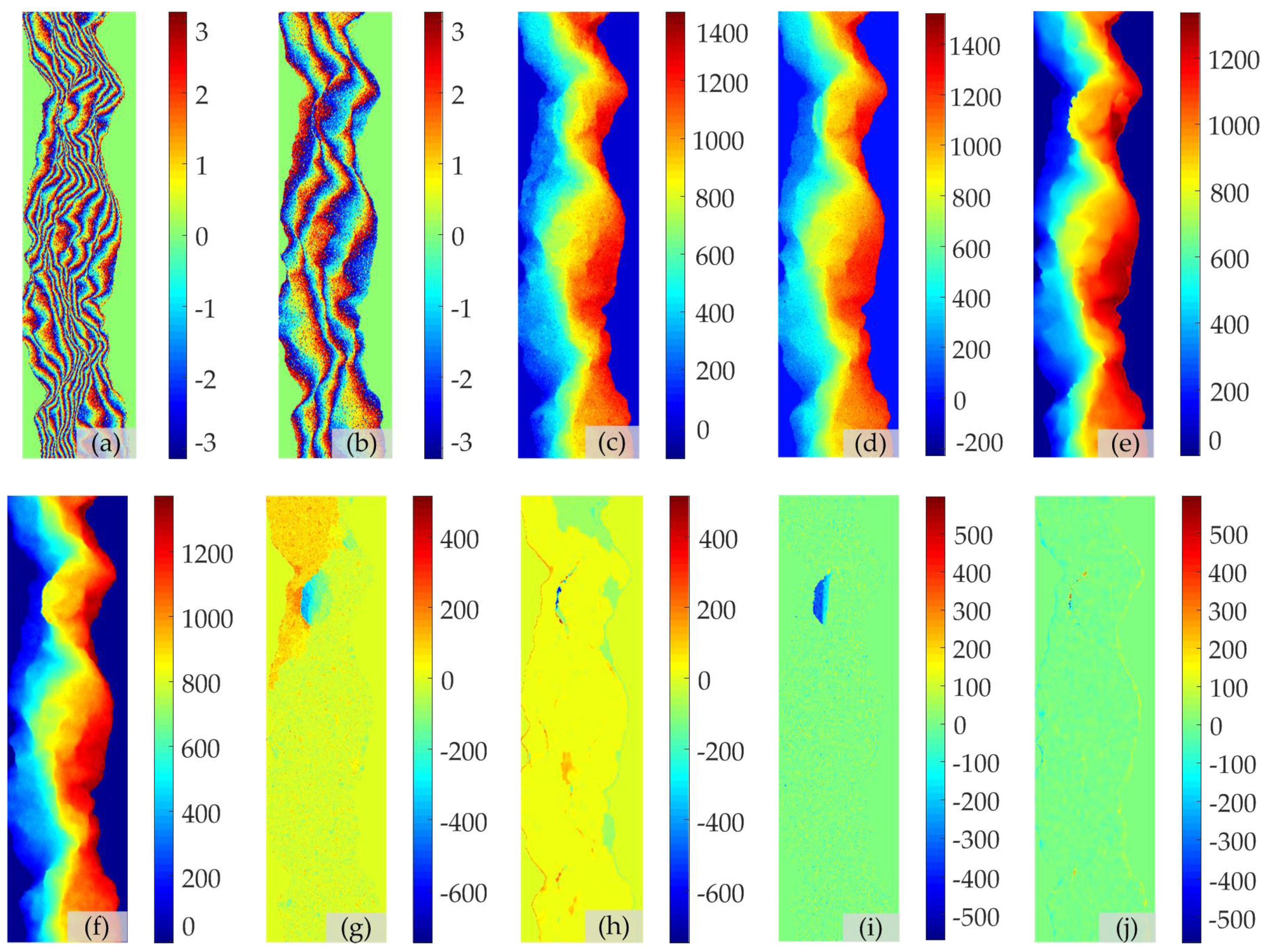
4.1. Validation Using Simulated Data

In the first experiment, the performance of the TSPA-UKFPU method is tested against the traditional TSPA on a simulated InSAR data set. Figure 4a displays the simulated DEM without noise. Figure 4b shows the simulated noise-free interferogram of Figure 4a with a long baseline, whereas Figure 4c shows a simulated noise-free interferogram of Figure 4a with a short baseline. The major interferometric parameters of these simulated data are listed in

Table 1. Major parameters of the simulated InSAR system.

Orbit Altitude	Incidence Angle	Wavelength
600 km	30°	0.24 m
Interferogram	Figure 4b	Figure 4c
Normal Baseline	389.20 m	112.10 m
Image Size	458 × 157 pixels	458 × 157 pixels

. Figure 4d illustrates the terrain height of Figure 4b obtained by the traditional TSPA method, while Figure 4e illustrates the terrain height of Figure 4b obtained by the TSPA-UKFPU method. It is worth mentioning that, to effectively and fairly compare the PU results, the same reference point, scale, and color range are used in the PU results obtained by the traditional TSPA method and the TSPA-UKFPU method of each pair of corresponding PU results to the maximum pixel value of those (the same approach is adopted hereinafter in experiments 2, 3 and 4). Figure 4d,e demonstrate that the TSPA and TSPA-UKFPU methods can obtain better DEM results when there is no noise. However, obvious differences are observable in the areas where the interferometric fringe changes drastically. Figure 4f shows the errors between Figure 4d and Figure 4a, and Figure 4g shows the errors between Figure 4e and Figure 4a. Figure 4f,g indicates that the TSPA-UKFPU method can obtain better results than the traditional TSPA method because the TSPA-UKFPU technique contains a gradient correction function that can effectively correct the gradient error estimated by the CRT. The $\tau$ values in Figure 4f,g are 0.21 and 0.18, respectively. TSPA-UKFPU clearly has a significantly higher PU accuracy than the traditional TSPA. In addition, TSPA-UKFPU uses only 7.28 s, and thus, it is 57.30% more efficient than the TSPA. This test therefore verifies that TSPA-UKFPU is more accurate and efficient than the traditional TSPA.

4.2. Robustness Analysis Using Simulated Data

In the second experiment, the robustness of the TSPA and TSPA-UKFPU is tested on the simulated interferograms shown in Figure 4b,c. We add hypergeometrically distributed noise of −4.34 dB and −0.25 dB to Figure 4b,c, respectively; the resulting interferometric noise phases are shown in Figure 5a,b. Figure 5c,d illustrate the terrain heights of Figure 5a,b, respectively, obtained by the traditional TSPA method. Similarly, Figure 5e,f illustrate the terrain heights of Figure 5a,b, respectively, obtained by the proposed TSPA-UKFPU method. Figure 5g shows the errors between Figure 5c and Figure 4a, whereas Figure 5h shows the errors between Figure 5e and Figure 4a, Figure 5i shows the errors between Figure 5d and Figure 4a, and Figure 5j shows the errors between Figure 5f and Figure 4a. Figure 5i,j shows that the short-baseline results of both the TSPA and the TSPA-UKFPU method do not distribute the PU error everywhere in the interferogram. In addition, TSPA-UKFPU exhibits a better noise robustness, and thus, the terrain heights estimated by the TSPA-UKFPU PU results are cleaner than those estimated by the TSPA. Figure 5g,h demonstrate that the PU errors of both the TSPA and the TSPA-UKFPU method are distributed. However, the area over which the PU error from TSPA-UKFPU is spread is smaller than that of the traditional TSPA method. The $\tau$ values in Figure 5g,h are 0.23 and 0.17, respectively, whereas the $\tau$ values in Figure 5i,j are 0.20 and 0.09, respectively. Moreover, compared with the TSPA, TSPA-UKFPU boasts a much faster execution speed. From the results of this test, we conclude that the proposed TSPA-UKFPU method is a more robust and effective MB PU method.

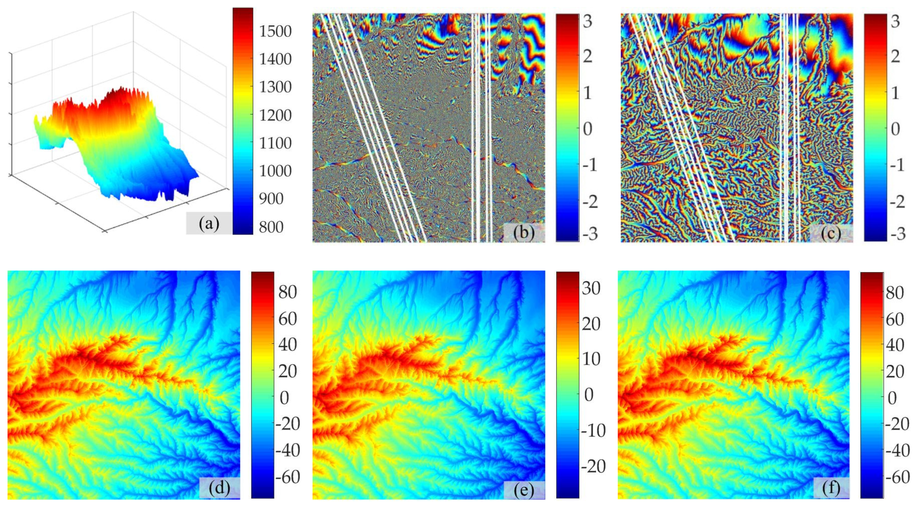
4.3. Validation Using Real Data

4.3.1. The Monostatic Data Set

In the third experiment, the performance of the TSPA-UKFPU method is tested on an Advanced Land Observing Satellite (ALOS) Phased Array-type L-band Synthetic Aperture Radar (PALSAR) monostatic MB InSAR data set. The major interferometric parameters of this real data set are listed in

Table 2. Major parameters of the employed Advanced Land Observing Satellite (ALOS) Phased Array type L-band Synthetic Aperture Radar (PALSAR) data.

Orbit Altitude	Incidence Angle	Wavelength
691.65 km	34.30°	0.2360 m
Interferogram	Figure 6b	Figure 6c
Normal Baseline	193.17 m	101.57 m
Image Size	800 × 800 pixels	800 × 800 pixels

. Figure 6a provides a 3-D display of the PALSAR DEM of the study area in the Himalayan mountain area. Figure 6b,c are filtered interferograms with different baseline lengths. Although the interferograms are filtered by the adapted filtering algorithm supplied by GAMMA, the interferograms still contain residual noise. In addition, the filtering algorithm may cause phase losses in the phase fringes of areas with dense topography changes. Since there are several mountains and valleys in the study area, the fringes of Figure 6b,c are complicated. Under these conditions, the phase continuity assumption may not work very well in the study area, i.e., it is difficult for the SB PU method to be effective in regions with steep fluctuations in the topography. Figure 6d,e show the PU results of Figure 6b obtained by the TSPA and TSPA-UKFPU methods, respectively. From Figure 6d, the TSPA will evidently produce significant PU errors in the phase fringes of dense topography changes and areas with residual noise. To further compare the PU results, we investigate the corresponding A and B regions in Figure 6d,e. Figure 6f,h show the corresponding A and B regions, respectively, in Figure 6d, while Figure 6g,i show the corresponding A and B regions, respectively, in Figure 6e. Figure 6f,h illustrate that the TSPA produces obvious PU errors and flaws due to pre-filtering and residual noise. However, because the TSPA-UKFPU technique not only boasts a better noise robustness but also contains a gradient correction function, the PU results in Figure 6g,i are smoother than those in Figure 6f,h. In this experiment, the TSPA consumes 1840.41 s, while the TSPA-UKFPU method consumes only 66.97 s. Accordingly, we can conclude that the PU accuracy and effectiveness of TSPA-UKFPU are better than those of the traditional TSPA method.

4.3.2. The Bistatic Data Set

In this section, the bistatic TerraSAR-X add-on for Digital Elevation Measurement (TanDEM-X) data are used to evaluate TSPA-UKFPU. Figure 7a illustrates a 3-D display of the TanDEM-X DEM of the study area, which is located in the city of Weinan, Shanxi Province, China. The major interferometric parameters of this real data set are listed in

Table 3. Major parameters of the employed TerraSAR-X add-on for Digital Elevation Measurement (TanDEM-X) data.

Orbit Altitude	Incidence Angle	Wavelength
514.8 km	36.60°	0.0320 m
Interferogram	Figure 7a	Figure 7b
Normal Baseline	−370.46 m	−127.79 m
Image Size	3040 × 2315 pixels	3040 × 2315 pixels

. Figure 7b,c show interferograms with different normal baseline lengths. Figure 7b was obtained on October 21, 2012, while Figure 7c was obtained from April 2, 2014. The white lines in Figure 7b,c are the Ice, Cloud, and Land Elevation Satellite (ICESat) tracks (elevation accuracy of approximately 14 cm). We use 1849 ICESat data points to verify the accuracies of the DEMs generated by different methods. To increase the PU difficulty, no filtering is performed during this experiment. This study area is geographically characterized by a great deal of rugged and mountainous terrain. In this case, the phase continuity assumption may not work very well; accordingly, it will potentially be challenging for SB PU to obtain the correct result. Figure 7d,e shows the absolute phases of Figure 7b,c, respectively, obtained by the TSPA method, whereas Figure 7f,g shows the absolute phases of Figure 7b,c, respectively, obtained by the TSPA-UKFPU method. In this experiment, we use the measurements obtained by ICESat as ground truth. To provide a clear display, we took 130 ICESat points and 200 ICESat points to show the results of the long and short baselines, respectively. The estimated elevations extracted from the PU results of the TSPA and TSPA-UKFPU methods are shown in Figure 7h,i. The elevations obtained by ICESat are also shown in Figure 7h,i. Ideally, the profiles of the elevations estimated from the two MB PU methods should be parallel with those acquired by ICESat, i.e., the more parallel the results are with the elevations measured by ICESat, the better the MB PU performance is. The standard deviation of the difference between the ICESat elevations and the TSPA-derived terrain heights are 3.25 m and 3.73 m for Figure 7b and Figure 7c, respectively, and that of the difference between the ICESat elevations and the TSPA-UKFPU-derived terrain heights are 3.07 m and 3.04 m for Figure 7b and Figure 7c, respectively. The estimated elevations obtained by TSPA-UKFPU generally agree better with the ICESat-derived elevation values. Moreover, the efficiency of TSPA-UKFPU in this experiment is 387.56 s, which is nearly 98.52% faster than the efficiency of the TSPA, which required 26,156.58 s.

5. Discussion

The proposed method is useful in global mapping. For example, the TanDEM DEM generated by the German Aerospace Center (DLR) uses the dual-baseline strategy to produce a global DEM. In 2011, the DLR collected data for the first time with a short-baseline (~200 m) global coverage. Subsequently, the DLR collected data globally for a second time in 2012 with a long baseline (~300 m) and then performed dual-baseline PU to improve the TanDEM-X global DEM accuracy. This indicates that the MB PU method has been applied in the reconstruction of high-precision DEMs. The MB PU method proposed in this paper not only can resolve the problems associated with steep gradient changes but also boasts a better noise robustness and contains a gradient estimation error correction function. Therefore, TSPA-UKFPU can be applied to the data processing of global DEMs generated in the future. Our results show that the research area of TanDEM-X that the area is mountainous and the terrain is undulated. In this case, the phase continuity assumption may not work very well, and thus, it will potentially be challenging for SB PU to obtain the correct result. In order to fairly compare the PU result, we introduced the classic SB SNAPHU for experimental comparison. In addition, we selected the corresponding ICESat data for accuracy evaluation. The standard deviation of the difference between the ICESat elevations and the SNAPHU-derived terrain heights are 4.62 m and 3.74 m for Figure 7b and Figure 7c, respectively. Although the TSPA does not need to obey the phase continuity assumption, the performance of this method is limited by its poor noise robustness and efficiency. Furthermore, the accuracies of the DEMs generated by the TSPA and TSPA-UKFPU are verified by ICESat elevation data; the long-baseline and short-baseline accuracies of the TSPA are 3.25 m and 3.73 m, respectively, while higher corresponding accuracies of 3.07 m and 3.04 m are obtained with TSPA-UKFPU. It can be seen that the elevations accuracies of TSPA and TSPA-UKFPU are significantly better than that of SNAPHU.

In addition, the proposed method can be applied to city surveying and mapping. The reconstruction of urban DEMs constitutes a research hotspot. Due to the large number and density of buildings in urban areas, the SB PU method cannot accurately reconstruct DEMs of such regions. Although some scholars have used the ML and MAP methods in the reconstruction of urban DEMs, the accuracy and effectiveness of these two methods are not ideal. In contrast, TSPA-UKFPU represents an MB PU method with a high noise robustness that can unwrap the interferometric phase by an efficient quality-guided strategy based on heap-sort. The PU strategy of heap-sort guarantees that the TSPA-UKFPU algorithm efficiently and accurately unwraps wrapped pixels along the paths from the high-reliability regions to the low-reliability regions of wrapped phase images. This strategy can enhance the reliability and efficiency of the PU method. Therefore, TSPA-UKFPU may be applied to the reconstruction of urban DEMs in the future.

The proposed method also has the potential to resolve the phase discontinuities encountered in surface deformation monitoring. Large gradient changes are common results of surface deformation; thus, the SB PU method cannot obtain good results for regions where the surface is severely deformed. However, the MB PU method does not need to obey the phase continuity assumption and may therefore be applied to deformation monitoring in the future to solve problems associated with the processing of data containing large gradient changes. TSPA-UKFPU not only boasts high noise robustness but also contains a better gradient correction function; therefore, in surface deformation monitoring, which commonly presents relatively high levels of noise, better results may be obtained.

The TSPA-UKFPU method proposed in this paper is one of the spatial domain phase unwrapping methods. There is another way to unwrap two sensitive phase maps which is temporal phase unwrapping by phase difference of two close-sensitivity interferometric phases [31]. In 2018, Manuel Servin et al. proposed a new temporal PU method. The method can use the non-wrapped phase difference to unwrap their highly-wrapped phase. However, the main drawback of close temporal phase-difference is that the phase-noise increases due to subtraction [32]. Moreover, one must take two close-sensitivity phase-measurements and simply multiplying their wrapped phase. The temporal method is a better PU method and has been well applied in the field of optics. We will try to apply the temporal PU method to the InSAR technology DEM production in future research.

However, some problems still need further study. For example, the phase gradient could be more accurately estimated with the CRT, and the UKF method could be employed to unwrap dense dead spots. The authors are working on these problems and hope to resolve them in the near future.

6. Conclusions

In this paper, an improved TSPA PU method is proposed that combines the UKF with an efficient quality-guided strategy based on heap-sort to improve the performance of the second stage of the original TSPA method. The results of the experiments demonstrate that the proposed TSPA-UKFPU method is an effective MB PU method. First, the proposed method uses step one of the TSPA to estimate the phase gradient using the CRT. Then, the range and azimuth gradients are filtered slightly using a median filter with better detail retention. Finally, the UKF model unwraps the interferometric phase by an efficient quality-guided strategy based on heap-sort. This PU strategy cannot only reduce the influence of noise on the unwrapped phase but also correct the PU errors caused by inaccurate gradient estimations.

A simulated DEM is used to perform two sets of simulated data experiments. The TSPA-UKFPU method contains a gradient correction function that can be employed to obtain better results, even in areas exhibiting complicated gradient changes. Noisy analog data are also processed by the TSPA and TSPA-UKFPU, and the results show that TSPA-UKFPU boasts a better noise robustness and gradient correction ability than the TSPA.

From the results of processing ALOS PALSAR data, the traditional TSPA will produce obvious flaws due to its poor noise robustness. However, the TSPA-UKFPU results are smoother than the TSPA results. The TanDEM-X images are located in Weinan of Shanxi Province, China, where the topography exhibits severe undulations. The accuracies of the DEMs generated by the different methods are evaluated by employing ICESat terrain data as ground truth. The results of the experiments demonstrate that TSPA-UKFPU represents an effective MB PU method. It is worth mentioning that, in comparison with the traditional TSPA method, although the TSPA-UKFPU method contains an extra filtering function, it cannot take the place of the traditional MB InSAR cascade processing framework. In other words, the TSPA-UKFPU method still prefers filtered input interferograms.

References

1. Yu, H.; Lan, Y. Robust two-dimensional phase unwrapping for multibaseline sar interferograms a two-stage programming approach. IEEE Trans. Geosci. Remote Sens. 2016, 54, 5217–5225. [Google Scholar] [CrossRef]
2. Ding, Z.; Wang, Z.; Lin, S.; Liu, T.; Zhang, Q.; Long, T. Local Fringe Frequency Estimation Based on Multifrequency InSAR for Phase-Noise Reduction in Highly Sloped Terrain. IEEE Geosci. Remote Sens. Lett. 2017, 14, 1527–1531. [Google Scholar] [CrossRef]
3. Yu, H.; Lan, Y.; Xu, J.; An, D.; Lee, H. Large-Scale L0-Norm and L1-Norm 2-D Phase Unwrapping. IEEE Trans. Geosci. Remote Sens. 2017, 55, 4712–4728. [Google Scholar] [CrossRef]
4. Pascazio, V.; Schirinzi, G. Multifrequency InSAR Height Reconstruction Through Maximum Likelihood Estimation of Local Planes Parameters. IEEE Trans. Image Process. 2002, 11, 1478–1489. [Google Scholar] [CrossRef]
5. Fornaro, G.; Monti Guarnieri, A.; Pauciullo, A.; De-Zan, F. Maximum likelihood multi-baseline SAR interferometry. In Proceedings of the 2006. IEE Proc. Radar Sonar Navig. 2006, 153, 279–288. [Google Scholar] [CrossRef]
6. Fornaro, G.; Pauciullo, A.; Sansosti, E. Phase difference-based multichannel phase unwrapping. IEEE Trans. Image Process. 2005, 14, 960–972. [Google Scholar] [CrossRef] [PubMed]
7. Ghiglia, D.C.; Wahl, D.E. Interferometric synthetic aperture radar terrain elevation mapping from multiple observations. In Proceedings of the 1994 IEEE Digital Signal Processing Workshop, Yosemite National Park, CA, USA, 2–5 October 1994; pp. 33–36. [Google Scholar]
8. Lombardo, P.; Lombardini, F. Multi-baseline SAR interferometry for terrain slope adaptivity. In Proceedings of the 1997 IEEE National Radar Conference, Syracuse, NY, USA, 13–15 May 1997; pp. 196–201. [Google Scholar]
9. Fornaro, G.; Pauciullo, A.; Sansosti, E. Bayesian approach to phase-difference-based phase unwrapping. In Proceedings of the 2002 IEEE 36th Asilomar Conference Signals, Systems and Computers, Pacific Grove, CA, USA, 3–6 November 2002; pp. 1391–1396. [Google Scholar]
10. Poggi, G.; Ragozini, A.R.P.; Servadei, D. A Bayesian Approach for SAR Interferometric Phase Restoration. In Proceedings of the 2000 IEEE International Geoscience and Remote Sensing Symposium, Honolulu, HI, USA, 24–28 July 2000; pp. 3202–3205. [Google Scholar]
11. Ying, L.; Munson, D.C.; Koetter, R.; Frey, B.J. Multibaseline InSAR terrain elevation estimation: A dynamic programming approach. In Proceedings of the 2003 International Conference on Image Processing, Barcelona, Spain, 14–17 September 2003; pp. 1522–4880. [Google Scholar]
12. Ferraiuolo, G.; Pascazio, V.; Schirinzi, G. Maximum a posteriori estimation of height profiles in InSAR imaging. IEEE Geosci. Remote Sens. Lett. 2004, 1, 66–70. [Google Scholar] [CrossRef]
13. Ferraioli, G.; Shabou, A.; Tupin, F.; Pascazio, V. Multichannel phase unwrapping with Graph-cuts. IEEE Geosci. Remote Sens. Lett. 2009, 6, 562–566. [Google Scholar] [CrossRef]
14. Baselice, F.; Ferraioli, G.; Pascazio, V.; Schirinzi, G. Contextual Information-Based Multichannel Synthetic Aperture Radar Interferometry: Addressing DEM reconstruction using contextual information. IEEE Signal Process. Mag. 2014, 31, 59–68. [Google Scholar] [CrossRef]
15. Ferraiuolo, G.; Federica, M.; Pascazio, V.; Schirinzi, G. DEM Reconstruction Accuracy in Multichannel SAR Interferometry. IEEE Trans. Geosci. Remote Sens. 2009, 47, 191–201. [Google Scholar] [CrossRef]
16. Yu, H.; Li, Z.; Bao, Z. A Cluster-Analysis-Based Efficient Multibaseline Phase-Unwrapping Algorithm. IEEE Trans. Geosci. Remote Sens. 2011, 49, 478–487. [Google Scholar] [CrossRef]
17. Jiang, Z.; Wang, J.; Song, Q.; Zhou, Z. A Refined Cluster-Analysis-Based Multibaseline Phase-Unwrapping Algorithm. IEEE Geosci. Remote Sens. Lett. 2017, 14, 1565–1569. [Google Scholar] [CrossRef]
18. Liu, H.; Xing, M.; Bao, Z. A Cluster-Analysis-Based Noise-Robust Phase-Unwrapping Algorithm for Multibaseline Interferograms. IEEE Trans. Geosci. Remote Sens. 2015, 45, 494–504. [Google Scholar] [CrossRef]
19. Xu, W.; Chang, E.C.; Kwoh, L.K.; Heng, A. Phase-unwrapping of SAR interferogram with multi-frequency or multi-baseline. In Proceedings of the 1994 IEEE International Geoscience and Remote Sensing Symposium, Pasadena, CA, USA, 8–12 August 1994; pp. 730–732. [Google Scholar]
20. Yuan, Z.; Deng, Y.; Li, F.; Wang, R.; Liu, G.; Han, X. Multichannel InSAR DEM Reconstruction Through Improved Closed-Form Robust Chinese Remainder Theorem. IEEE Geosci. Remote Sens. Lett. 2013, 10, 1314–1318. [Google Scholar] [CrossRef]
21. Wang, W.; Xia, X. A Closed-Form Robust Chinese Remainder Theorem and Its Performance Analysis. IEEE Trans. Image Process. 2010, 58, 5655–5666. [Google Scholar] [CrossRef] [Green Version]
22. Li, X.; Xia, X. A Fast robust Chinese remainder theorem based phase unwrapping algorithm. IEEE Trans. Signal Process. Lett. 2008, 15, 665–668. [Google Scholar] [CrossRef]
23. Thompson, D.G.; Robertson, A.E.; Arnold, D.V.; Long, D.G. Multi-baseline interferometric SAR for iterative height estimation. In Proceedings of the 1999 IEEE International Geoscience and Remote Sensing Symposium, Hamburg, Germany, 28 June–2 July 1999; pp. 251–253. [Google Scholar]
24. Gao, Y.; Zhang, S.; Li, T.; Chen, Q.; Li, S.; Meng, P. Adaptive Unscented Kalman Filter Phase Unwrapping Method and Its Application on Gaofen-3 Interferometric SAR Data. Sensors 2018, 18, 1793. [Google Scholar] [CrossRef]
25. Xie, X.; Dai, G. Unscented information filtering phase unwrapping algorithm for interferometric fringe patterns. Appl. Opt. 2017, 56, 9423–9434. [Google Scholar] [CrossRef]
26. Kim, M.G.; Griffiths, H.D. Phase unwrapping of multibaseline interferometry using Kalman filtering. In Proceedings of the 7th 1999 International Conference on Image Processing and Its Applications, February Manchester, UK, 13–15 July 1999; pp. 813–817. [Google Scholar]
27. Xie, X.; Pi, Y. Multi-baseline phase unwrapping algorithm based on the unscented Kalman filter. IET Radar Sonar Navig. 2011, 5, 296–304. [Google Scholar] [CrossRef]
28. Xie, X. Multi-baseline UKF phase unwrapping algorithm via joint phase slope estimator. IEICE Commun. Express 2014, 3, 20–26. [Google Scholar] [CrossRef] [Green Version]
29. Chen, R.; Yu, W.; Wang, R.; Liu, G.; Shao, Y. Integrated Denoising and Unwrapping of InSAR Phase Based on Markov Random Fields. IEEE Trans. Geosci. Remote Sens. 2013, 51, 4473–4485. [Google Scholar] [CrossRef]
30. Bioucas-Dias, J.M.; Valadão, G. Phase Unwrapping via Graph Cuts. IEEE Trans. Image Process. 2007, 16, 698–709. [Google Scholar] [CrossRef] [PubMed] [Green Version]
31. Wyant, J.C. Testing aspherics using two-wavelength holography. Appl. Opt. 1971, 10, 2113–2118. [Google Scholar] [CrossRef] [PubMed]
32. Servin, M.; Padilla, M.; Garnica, G. Super-sensitive two-wavelength fringe projection profilometry with 2-sensitivities temporal unwrapping. Opt. Lasers Eng. 2018, 106, 68–74. [Google Scholar] [CrossRef] [Green Version]
Figure 1. (a) Simulated interferogram with long normal baseline. (b) Simulated interferogram with short normal baseline. (c) Horizontal gradient obtained by the single-baseline (SB) phase unwrapping (PU) of (b). (d) Vertical gradient obtained by the SB PU of (b). (e) Horizontal gradient obtained by the two-stage programming approach (TSPA) of (b). (f) Vertical gradient obtained by the TSPA of (b).
Remotesensing 11 00199 g001
Figure 2. Two-dimensional grid associated with the interferometric phase signal.
Remotesensing 11 00199 g002
Figure 3. Schematic representation of the proposed two-stage programming approach (TSPA)- unscented Kalman filter phase unwrapping (UKFPU) method.
Remotesensing 11 00199 g003
Figure 4. (a) Employed Digital elevation model (DEM) (unit: m). (b) Simulated interferogram with long normal baseline. (c) Simulated interferogram with short normal baseline. (d) Terrain height estimated by the phase unwrapping (PU) result of the two-stage programming approach (TSPA) method. (e) Terrain height estimated by the PU result of the TSPA- unscented Kalman filter (UKF) PU method. (f) Errors between (d) and (a). (g) Errors between (e) and (a).
Remotesensing 11 00199 g004
Figure 5. (a) Simulated interferogram with long normal baseline. (b) Simulated interferogram with short normal baseline. (c) Terrain height estimated result of (a) obtained by the two-stage programming approach (TSPA) method. (d) Terrain height estimated result of (b) obtained by the TSPA method. (e) Terrain height estimated result of (a) obtained by the TSPA–unscented Kalman filter phase unwrapping (UKFPU) method. (f) Terrain height estimated result of (b) obtained by the TSPA–UKFPU method. (g) Errors between Figure 4a and Figure 5c. (h) Errors between Figure 4a and Figure 5e. (i) Errors between Figure 4a and Figure 5d. (j) Errors between Figure 4a and Figure 5f.
Remotesensing 11 00199 g005
Figure 6. (a) 3-D display of the Advanced Land Observing Satellite (ALOS) Phased Array type L-band Synthetic Aperture Radar (PALSAR) digital elevation models (DEM). (b) Real interferogram with long normal baseline. (c) Real interferogram with short normal baseline. (d) PU result of (b) obtained by two-stage programming approach (TSPA). (e) Phase unwrapping (PU) result of (b) obtained by TSPA- unscented Kalman filter (UKF)PU. (f) PU solution of the rectangular A region in (d). (g) PU solution of the rectangular A region in (e). (h) PU solution of the rectangular B region in (d). (i) PU solution of the rectangular B region in (e).
Remotesensing 11 00199 g006
Figure 7. (a) 3-D display of TerraSAR-X add-on for Digital Elevation Measurement (TanDEM-X) digital elevation models (DEM). (b) Real interferogram with long normal baseline. (c) Real interferogram with short normal baseline. (d) Phase unwrapping (PU) result of (a) obtained by two-stage programming approach (TSPA). (e) PU result of (b) obtained by TSPA. (f) PU result of (a) obtained by TSPA-UKFPU. (g) PU result of (b) obtained by TSPA- unscented Kalman filter (UKF)PU. (h) The ICESat elevation results of (b) obtained by different method. (i) The portion elevation results of (c) obtained by different methods.
Remotesensing 11 00199 g007aRemotesensing 11 00199 g007b