Combination Analysis of Future Polar-Type Gravity Mission and GRACE Follow-On

Abstract

Thanks to the unprecedented success of Gravity Recovery and Climate Experiment (GRACE), its successive mission GRACE Follow-On (GFO) has been in orbit since May 2018 to continue measuring the Earth’s mass transport. In order to possibly enhance GFO in terms of mass transport estimates, four orbit configurations of future polar-type gravity mission (FPG) (with the same payload accuracy and orbit parameters as GRACE, but differing in orbit inclination) are investigated by full-scale simulations in both standalone and jointly with GFO. The results demonstrate that the retrograde orbit modes used in FPG are generally superior to prograde in terms of gravity field estimation in the case of a joint GFO configuration. Considering the FPG’s independent capability, the orbit configurations with 89- and 91-degree inclinations (namely FPG-89 and FPG-91) are further analyzed by joint GFO monthly gravity field models over the period of one-year. Our analyses show that the FPG-91 basically outperforms the FPG-89 in mass change estimates, especially at the medium- and low-latitude regions. Compared to GFO & FPG-89, about 22% noise reduction over the ocean area and 17% over land areas are achieved by the GFO & FPG-91 combined model. Therefore, the FPG-91 is worthy to be recommended for the further orbit design of FPGs.

1. Introduction

The Earth is undergoing complicated and continuous mass transport [1]. To better quantify the mass changes, the Gravity Recovery and Climate Experiment (GRACE) mission was launched in 2002, which consists of the twin satellites flying in the same near-polar orbit at about 500-km altitude and separated by 220 km [2]. The key technology that enables GRACE to observe large-scale mass variations near the Earth surface is the onboard K-band microwave ranging system (KBR), which delivers inter-satellite range measurements with an accuracy at micron level to precisely capture orbit perturbation differences between the two GRACE satellites caused by heterogeneous mass distribution of the Earth [2,3]. Along with the KBR, other important sensors onboard GRACE satellites include Global Positioning System (GPS) receivers for precise orbit determination (POD), high-precision accelerometers for measuring non-gravitational forces and star cameras for attitude determination [4,5,6]. Based on the precise data collected by the above sensors, many scientific institutions have produced high-quality static and temporal gravity field models [7,8,9,10,11], which are successfully adopted for quantitative researches concerning the Earth’s mass changes, such as global mean sea-level variations [12,13], continental water balance [14,15], and the Tibetan Plateau and Antarctic regional ice losses [16,17].

In view of such a great success achieved by GRACE in terms of the Earth’s mass change exploration, its successor GRACE Follow-On (GFO) was launched on 22 May 2018 to continue providing the geodetic observation records [18,19]. As a demonstrator, GFO carries a laser ranging interferometer (LRI) for measuring inter-satellite ranges with an accuracy level of a few tens nanometers in addition to the sensors onboard the GRACE satellites [18,19,20]. However, even with such a dramatic accuracy improvement for the range observations, some full-scale pre-launch simulations indicated that only a moderate improvement on gravity field estimation can be reached by GFO as compared to GRACE [18,21]. The dominant barrier to further improvement on gravity field determination by GFO is the temporal aliasing issue, which is more intractable than other limiting factors in the GFO error budget [18,21].

From a digital signal processing aspect, aliasing is due to undersampling of the signal to be recovered. According to the Nyquist sampling theorem, when sampling frequency is smaller than twice of the original signal frequency, aliasing definitely occurs [22]. In terms of GRACE monthly gravity field recovery, temporal aliasing is mainly attributed to those high-frequency signals originating from the oceanic tidal variations at daily or sub-daily scale, as well as the short-term energy exchange process (generally within a few hours) between atmosphere and ocean [23,24]. Because of the limited bandwidth for observations and sparse ground track of GRACE, most part of these signals typically need to be reduced by priori background models during gravity field recovery process [25], which are, however, subject to errors [26,27]. Therefore, the remaining high-frequency signals result in the temporal aliasing errors in monthly-average gravity solutions, which manifest themselves as the typical north-south stripes in spatial pattern of unfiltered GRACE models [28,29].

To mitigate the troublesome temporal aliasing effects, post-processing filtering techniques are generally applied as a standard procedure [28,29,30]. However, the fundamental solution should be based on the enhanced signal sampling and gravity field modelling strategy [31,32,33,34]. One of the most straightforward and efficient ways is to increase the number of satellites in space for denser sampling of gravity signals. Thereby, many researchers have investigated novel concepts of satellite formation flight (SFF) or satellite constellations dedicated to gravity field recovery, including the cartwheel, pendulum, and Bender-type configurations [35,36,37,38,39]. Among all, the Bender-type SFF, formed by two pairs of GRACE-type inline satellites (in polar and inclined orbits), is most promising from both technological and economic aspects. Therefore, it is selected as the primary candidate for the Next Generation Gravity Mission (NGGM) concepts [40,41] by the European Space Agency (ESA). During the service period of GFO, other Future Polar-type Gravity mission (FPG) will be probably launched [42]. Therefore, the primary motivation of this article is to investigate the optimal FPG orbit configuration in combination with GFO, under the precondition that the FPG has the same payload accuracy as GRACE and comparable capability of recovering global static and temporal gravity fields to GRACE. With this in mind, the search space for FPG’s key orbit elements (i.e., orbit altitude and inclination) is greatly reduced. Considering a five-year nominal mission lifetime for FPG, its orbit altitude is similar to GRACE. As such, the emphasis of FPG orbit adjustment will be put on the orbit inclination selection issue.

The rest of this article is organized as follows. Section 2 presents the details of full-scale simulations for FPG orbit selection and performance evaluation. Gravity field results from the standalone FPG, with different inclinations, and jointly with GFO are demonstrated in Section 3. In Section 4, we explain the underlying mechanism of the presented results and further discuss the practical consideration of FPG orbit design. Conclusions are given in Section 5.

2. Numerical Simulation Scheme

2.1. Mathematical Model for Gravity Field Recovery

The dynamic approach is adopted in our gravity field model recovery [43], which is widely used in real GRACE data processing by different scientific institutions [7,8,44,45,46]. In this section, we outline basic formulas of the dynamic approach used in the article, as well as relevant references for more detailed descriptions.

The Earth gravity field model can be expressed via a set of Spherical Harmonic Coefficients (SHC) $u=\left\{{\overline{C}}_{lm},{\overline{S}}_{lm}\right\}$ with following Spherical Harmonic (SH) expansion,

$$V(\rho ,\phi ,\lambda ;u)=\frac{GM}{\rho }\left[1+{\displaystyle \sum _{l=2}^{L_{MAX}}{\displaystyle \sum _{m=0}^l{(\frac{R_E}{\rho })}^l({\overline{C}}_{lm}\cos m\lambda +{\overline{S}}_{lm}\sin m\lambda )}}\cdot {\overline{P}}_{lm}(\sin \phi )\right]$$

(1)

where $V$ is the gravitational potential of an arbitrary point on or outside the Earth with the spherical coordinate of radius $\rho$, latitude $\phi$ and longitude $\lambda$, in the Earth-fixed frame. GM is the product of the gravitational constant and the Earth mass, and $R_E$ is the Earth’s mean equatorial radius; l and m stand for the degree and order of SH expansion, respectively, with $L_{MAX}$ being the maximum degree of the expansion; ${\overline{P}}_{lm}$ is the fully normalized associate Legendre function of degree l and order m.

The estimation of SHC $u$ from satellite observations is based on the Newton’s law of motion [47], which is formulated as a three-dimensional second-order nonlinear ordinary differential equation (ODE),

$$\ddot{r}(t)=a(t;r\left(t\right),\dot{r}\left(t\right),p,u)$$

(2)

where $r\left(t\right)$, $\dot{r}\left(t\right)$, and $\ddot{r}\left(t\right)$ denote the vectors of satellite’s position, velocity and acceleration at epoch t, respectively. $a$ is the force acting on the unit mass of the satellite, where $p$ represents the parameters vector for the force models except the Earth gravity field. In the case of GRACE, $p$ is referred to accelerometer calibration parameters (e.g., bias and scale parameters) [48]. When the force models are given, the position and velocity of satellite’s orbit are determined as follows [49],

$$\{\begin{array}{l}r(t)=r(t_0)+(t-t_0)\cdot \dot{r}(t_0)+{\displaystyle {\int }_{t_0}^t{\displaystyle {\int }_{t_0}^{\tau }a({\tau }^{\prime };r({\tau }^{\prime }),\dot{r}({\tau }^{\prime }),p,u}})d{\tau }^{\prime }d\tau \\ \dot{r}(t)=\dot{r}(t_0)+{\displaystyle {\int }_{t_0}^{t}a(\tau ;r(\tau ),\dot{r}(\tau ),p,u)d\tau }\end{array}$$

(3)

where ${(r^T(t_0),{\dot{r}}^T(t_0))}^T$ denote the position and velocity vectors at initial epoch $t_0$ of an orbit arc. According to Equation (3), the position and velocity vectors at any epoch t within the orbit arc are the function of parameter vector $x={(w^T,u^T)}^T$, where $w={(r^T(t_0),{\dot{r}}^T(t_0),p^T)}^T$ is the arc-specific parameters vector. Linearizing the Equation (3) with respect to the approximate vector $x_0$ of parameters, we have,

$$\{\begin{array}{l}r(t)=r^{REF}(t)+\frac{\partial r^{REF}(t)}{\partial x_0}\delta x\\ \dot{r}(t)={\dot{r}}^{REF}(t)+\frac{\partial {\dot{r}}^{REF}(t)}{\partial x_0}\delta x\end{array}$$

(4)

where the vectors of position $r^{REF}(t)$ and velocity ${\dot{r}}^{REF}(t)$, named as the reference orbit, are numerically integrated with Equation (3) by replacing $x$ with $x_0$. $\delta x$ is the correction vector to $x_0$. Substituting $r(t)=r^{OBS}(t)+v_r\left(t\right)$ into the first equation of Equation (4), we get the observational equation for position at epoch t,

$$v_r(t)=\frac{\partial r^{REF}(t)}{\partial x_0}\delta x-\left[r^{OBS}(t)-r^{REF}(t)\right]=\frac{\partial r^{REF}(t)}{\partial x_0}\delta x-\Delta r(t)$$

(5)

where $r^{OBS}(t)$ and $v_r\left(t\right)$ represent the position observation and its correction at epoch t. The inter-satellite range rate $\dot{\rho }\left(t\right)$ between GRACE-A and B can be expressed as,

$$\dot{\rho }\left(t\right)=e_{AB}^T\left(t\right){\dot{r}}_{AB}\left(t\right)$$

(6)

where, the subscripts A and B denote the values of GRACE-A and B, ${\dot{r}}_{AB}(t)={\dot{r}}_B(t)-{\dot{r}}_A(t)$ is the velocity difference vector and $e_{AB}(t)=r_{AB}(t)/\sqrt{r_{AB}^T(t)r_{AB}(t)}$ with $r_{AB}=r_B-r_A$. By substituting $\dot{\rho }(t)={\dot{\rho }}^{OBS}(t)+v_{\dot{\rho }}(t)$ and the second equation of Equation (4) into Equation (6) for both GRACE-A and B, we get the following observational equation for range rate measurement at epoch t,

$$v_{\dot{\rho }}(t)=\frac{\partial {\dot{\rho }}^{REF}(t)}{\partial x_0}\delta x-\left[{\dot{\rho }}^{OBS}(t)-{\dot{\rho }}^{REF}(t)\right]=\frac{\partial {\dot{\rho }}^{REF}(t)}{\partial x_0}\delta x-\Delta \dot{\rho }(t)$$

(7)

where, ${\dot{\rho }}^{REF}(t)$ is computed with the reference orbit, ${\dot{\rho }}^{OBS}(t)$ and $v_{\dot{\rho }}(t)$ stand for the range rate observation and its correction, respectively. The partial derivatives $\frac{\partial r^{REF}(t)}{\partial x_0}$ and $\frac{\partial {\dot{r}}^{REF}(t)}{\partial x_0}$ are numerically integrated by solving the so-called ‘variational equation’ and $\frac{\partial {\dot{\rho }}^{REF}(t)}{\partial x_0}$ is the combination of them, which can be referred to [50] (pp. 240–243), [51] (pp. 30–32) and [49] for detailed descriptions. The observational equations in the form of Equations (5) and (7) for all epochs within one arc, i.e., arc j, are collected together and briefly expressed in the following form,

$$v_j=A_j\delta x_j-y_j=\left(\begin{array}{cc}{A}_{w_j}& A_{u_j}\end{array}\right)\left(\begin{array}{c}\delta w_j\\ \delta u\end{array}\right)-y_j$$

(8)

where $v_j$ denotes the vector of all corrections, $A_j$, $A_{w_j}$ and $A_{u_j}$ are the design matrices, and $y_j$ is the vector of all constant terms of the arc j. The Normal Equation (NEQ) of the arc based least squares adjustment is derived as [48],

$$\left(\begin{array}{cc}{N}_{w_j{w}_j}& N_{w_j{u}_j}\\ N_{w_j{u}_j}^T& N_{u_j{u}_j}\end{array}\right)\left(\begin{array}{c}\delta w_j\\ \delta u\end{array}\right)=\left(\begin{array}{c}{R}_{w_j}\\ R_{u_j}\end{array}\right)$$

(9)

where $N_{w_j{w}_j}=A_{w_j}^T{P}_j{A}_{w_j}$, $N_{u_j{u}_j}=A_{u_j}^T{P}_j{A}_{u_j}$, $N_{w_j{u}_j}=A_{w_j}^T{P}_j{A}_{u_j}$ and $R_{w_j}=A_{w_j}^T{P}_j{y}_j$, $R_{u_j}=A_{u_j}^T{P}_j{y}_j$. $P_j$ denotes the weight matrix constructed based on the precision of observations. To recover $\delta u$ with observations of multiple arcs, such as one month, the arc-specific parameters $\delta w_j$ should be pre-eliminated arc-wise, forming the reduced normal equation. After that, reduced normal equations are summed up to J arcs, and then the SHC parameter $\delta u$ is obtained by solving Equation (10),

$${\tilde{N}}_J\cdot \delta u={\tilde{R}}_J$$

(10)

where ${\tilde{N}}_J={\displaystyle \sum _J{\tilde{N}}_j}$ and ${\tilde{R}}_J={\displaystyle \sum _J{\tilde{R}}_j}$. ${\tilde{N}}_j$ and ${\tilde{R}}_j$ are coefficient matrix and the right-hand side of the reduced normal equation of arc j, with ${\tilde{N}}_j=N_{u_j{u}_j}-N_{w_j{u}_j}^T{N}_{w_j{w}_j}^{-1}{N}_{w_j{u}_j}$ and ${\tilde{R}}_j=R_{u_j}-N_{w_j{u}_j}^T{N}_{w_j{w}_j}^{-1}{R}_{w_j}$ [48].

As regard to the GFO and FPG combination, it can be carried out on NEQ level by Equation (11),

$$({\tilde{N}}_J^{GFO}+{\tilde{N}}_J^{FPG})\cdot \delta u=({\tilde{R}}_J^{GFO}+{\tilde{R}}_J^{FPG})$$

(11)

where ${\tilde{N}}_J^{GFO}$, ${\tilde{R}}_J^{GFO}$ and ${\tilde{N}}_J^{FPG}$, ${\tilde{R}}_J^{FPG}$ are established by Equation (10) of GFO and FPG, respectively. It should be mentioned here that the same variance of unit weight must be employed in constructing the weight matrices of GFO and FPG, otherwise the two normal equations cannot be simply summed up as in Equation (11).

2.2. Orbit Configuration Selection for FPG

In gravity field recovery, the orbit altitude and inclination play the key role [52] (pp. 41–43). Since the gravity signals attenuate rapidly with the increase of orbit altitude [47], the ideal gravimetric satellite should fly as low as possible in order to be sufficiently sensitive to the signals. However, the lower altitude of the satellite, the stronger atmospheric drag acting on it, which requires more fuels to maintain the mission operation and thus shortens its lifetime [37]. As regard to the orbit inclination, it could not be better to select the 90-degree inclination for a global coverage of the Earth. However, due to the launch limit, it is a challenge to put satellites in an exact polar orbit. For example, GRACE was flying in a near-polar orbit with 89-degree inclination, which left two 1-degree-radius circles in the south and north poles (namely the polar gaps). In general, a large polar gap will significantly impact the estimation of zonal SHC and eventually corrupt the estimated gravity field. The maximum recoverable degree and order (d/o) of SHC in the case of a given g-degree polar gap can be roughly calculated via dividing 180 (degree) by g [51] (p. 205).

Considering the twin satellites of GFO separated by 220 km both in the near-circular orbit of 490-km altitude and 89-degree inclination [18], its initial orbit configuration in the following simulations will be kept fixed as listed in

Table 1. Initial orbit configurations of GFO and FPG for simulation study

Orbit Configuration	Altitude (km)	Inclination (deg.)	Eccentricity	Inter-Satellite Distance (km)
GFO	490	89	0.0015	220
FPG-87	500	87	0.0015	220
FPG-89		89
FPG-91		91
FPG-93		93

. In consideration of a nominal five-year mission lifetime, the FPG initial orbit altitude is currently supposed to be the same as GRACE (namely 500 km) [2]. With regard to the inclination choice of FPG, the relationship between the polar gap and the maximum recoverable SHC d/o, as mentioned above, should be taken into consideration. For typical monthly temporal gravity field model up to 60 d/o, it requires the polar gap smaller than 3 degrees, while for static gravity field models up to 180 d/o, the polar gap should be within 1 degree in theory. Once the polar gap size is determined, there exist two kinds of orbits, namely the prograde orbit (inclination smaller than 90 degrees) and the retrograde orbit (inclination larger than 90 degrees) [53] (p. 99). For example, the previously dedicated gravity missions CHAllenging Mini-satellite Payload (CHAMP) (87-degree inclination) [54] and GRACE (89-degree inclination) are in prograde orbits, while Gravity field and steady-state Ocean Circulation Explorer (GOCE) (96.5-degree inclination) [55] is in a retrograde orbit. In general, the retrograde-orbit satellites require more fuel than the prograde ones during launch in order to overcome the Earth’s rotation speed, but it is not a technical problem to launch either prograde or retrograde satellites.

In the following simulation study, we preliminarily select four sets of FPG configurations, which differ only in orbit inclinations. Their initial orbit elements are listed in Table 1 and denoted as FPG-87, FPG-89, FPG-91, and FPG-93 (corresponding to the inclinations of 87, 89, 91, and 93 degrees, respectively). Note that the initial Right Ascension of Ascending Nodes (RAAN) are selected as 0 degree for GFO, FPG-87, FPG-91, and FPG-93 while 180 degrees for FPG-89, which is designed to avoid the nearly full overlay of ground tracks of GFO and FPG-89 when combining the two [32]. The initial inter-satellite distances for all GFO and FPG configurations are fixed as 220 km.

2.3. Numerical Simulation Procedures

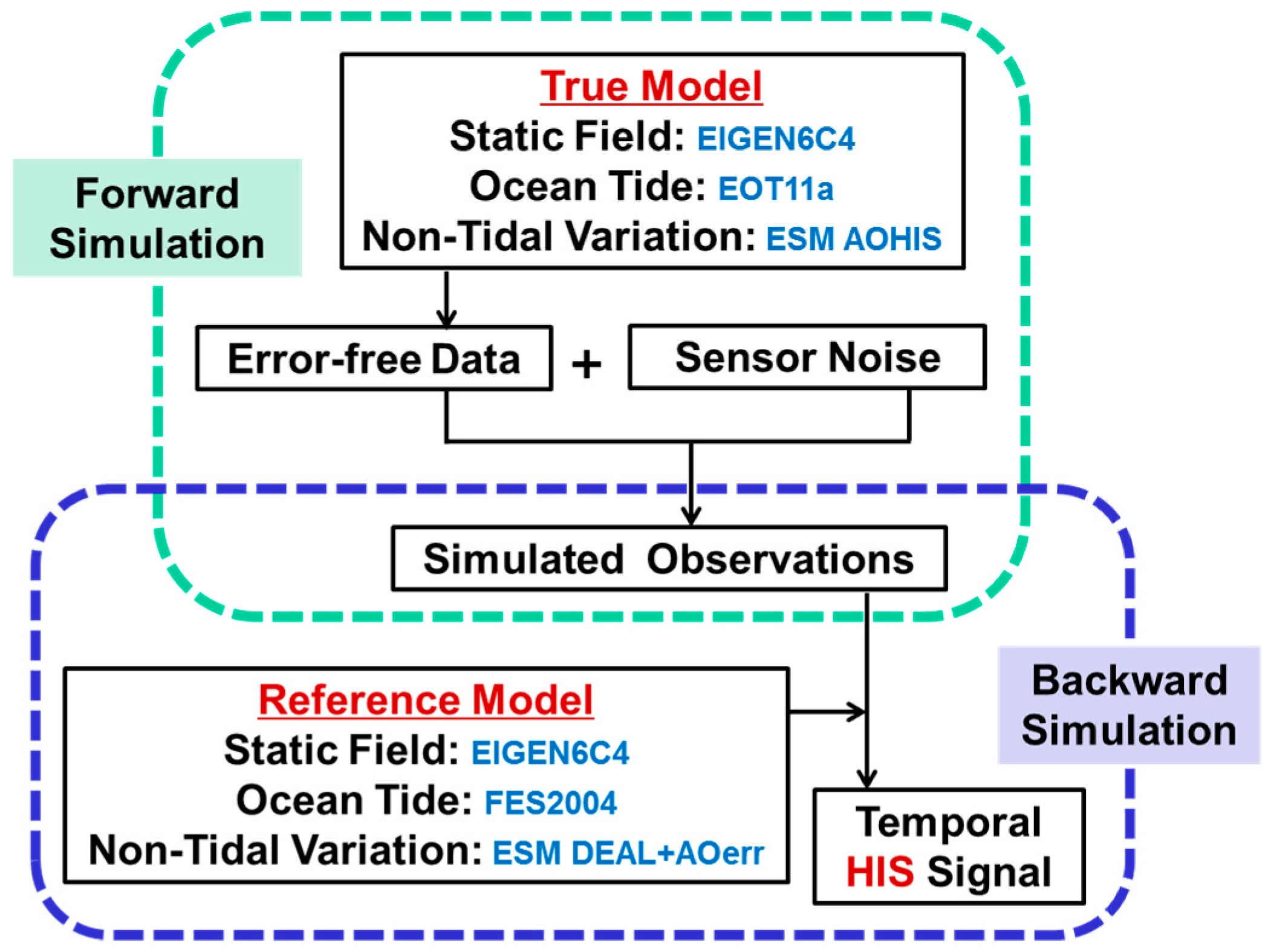
The simulation procedures involving the forward and the backward simulation steps [18] are shown in Figure 1. In the forward simulation step, we apply a set of true background models to generate the simulated observations. The true background models are listed in

Table 2. Background models for numerical simulation. True models are used for simulated observations generation while the reference models are applied to gravity field recovery.

Force Categories	True Model	Reference Model
Static Field	EIGEN6C4 (100 d/o)	EIGEN6C4 (100 d/o)
Ocean Tide	EOT11a (100 d/o)	FES2004 (100 d/o)
Non-tidal Variation	ESM AOHIS (100 d/o)	ESM DEAL + AOerr (100 d/o)

, where EIGEN6C4 [56] is used as the true static gravity field model and EOT11a (including main wave and interpolated secondary wave) [57] is treated as the true ocean tide model. For non-tidal variation signals, the AOHIS component of ESM is adopted to represent the integrated signal of atmosphere (A), oceans (O), terrestrial hydrological water (H), continental ice-sheets (I), and the solid earth (S) [24]. The maximum degree and order for all models is chosen as 100 [18]. Given the initial orbit elements defined in Table 1, the satellite orbits for both GFO and FPG can be generated by numerical integration [50] (pp. 117–146). The combined eighth-order Runge–Kutta and eighth-order Gauss–Jackson integrator with an integration step of 5 s is applied to generate the error-free data, which include satellite orbit positions and inter-satellite range-rates. To produce more realistic observations, above error-free data should be added with sensor noises. In this work, the sensor noises are treated as Gaussian white noise with zero expectation [31,32], while more sophisticated noise models can be found in [58]. The standard deviations (SD) of major onboard sensors’ noises, listed in

Table 3. The standard deviations (SD) of white Gaussian sensor noises used for the generation of simulated observations

Obs. Type	Orbit Pos.	GFO/FPG-KBR	GFO-LRI	Accelerometer
SD Value	1 cm	0.2 μm/s	10 nm/s	0.3 nm/s2

, are based on their performances in real GRACE data. As shown, 1-cm SD is selected for orbit positions [31,32,33]. With regard to the range-rate data, we add noise with SD of 0.2 μm/s to KBR measurements in GFO and FPG [18,45], while with SD of 10 nm/s to LRI measurements in GFO [18]. Although the non-gravitational forces are not simulated during orbit integration, the accelerometer’s noise with SD of 0.3 nm/s² is directly simulated during the integration of orbit [52] (pp. 50–51). We simulate full-year observations in 2006 for all orbit configurations, which are subsequently used in the backward simulation step for gravity field model recovery.

In the backward simulation step, we recover the monthly gravity field model up to 100 d/o [18] by the dynamic approach using above simulated observations. For parameterizations, we choose the orbit arc length as 6 h for the initial position and velocity estimation [44,45,46], and estimate the accelerometer parameters (bias and linear drift) every 1.5 h (orbital period) [45]. Observations’ weight matrices in Equation (9) are constructed based on corresponding SD values listed in Table 3 with the same variance of unit weight. The reference background models, used for reference orbit and partial derivatives integration in Equations (5) and (7), are listed in Table 2. As shown, FES2004 [59] is applied as reference ocean tide model, and DEAL plus AOerr components of ESM [27] are used to represent the AO components of AOHIS in true background models [24]. Since the emphasis of the article is on temporal gravity model recovery, the true and reference static models are identical [21,33,35]. The differences between true and reference background models are designed to introduce the temporal aliasing errors to the recovered gravity model [18,21,33,37]. As shown in Figure 1, the temporal signal we want to recover in each monthly model is the average HIS of this month, which is the integrated signal of terrestrial hydrological water (H), continental ice-sheets (I), and the solid earth (S) [18,24].

2.4. Evaluation Metrics for Recovered Gravity Field Model

In a simulated world, the quality of the recovered gravity field model can be easily evaluated by comparing the true and the recovered fields. In this article, the evaluation metrics for recovered gravity field models are derived based on monthly SHC differences $\left\{\Delta C_{lm},\Delta S_{lm}\right\}$, which are calculated by subtracting the recovered model from the true static model (EIGEN6C4 100 d/o) plus the true monthly HIS signal (100 d/o) as shown in Equation (12) according to [18],

$$\Delta C_{lm}={\overline{C}}_{lm}^{EIGEN6C4+HIS}-{\overline{C}}_{lm}^{REC},\hspace{1em}\Delta S_{lm}={\overline{S}}_{lm}^{EIGEN6C4+HIS}-{\overline{S}}_{lm}^{REC}$$

(12)

where the superscripts EIGEN6C4, HIS, and REC represent the SHC from EIGEN6C4, monthly HIS and the recovered models in simulations. Given SHC differences, the degree geoid height error (DGHE) and cumulative geoid height error (CGHE) of the recovered model can be calculated by

$$\begin{array}{l}DGHE(n)=R_E\cdot \sqrt{{\displaystyle \sum _{m=0}^l(\Delta C_{lm}^2+\Delta S_{lm}^2)}},\hspace{1em}(l=n)\\ CGHE(n)=R_E\cdot \sqrt{{\displaystyle \sum _{l=2}^n{\displaystyle \sum _{m=0}^l(\Delta C_{lm}^2+\Delta S_{lm}^2)}}}\end{array}$$

(13)

where $DGHE(n)$ represents the DGHE of degree n and $CGHE(n)$ represents the CGHE up to degree n. One can also construct spatial-domain metrics by the spatial differences plot (SDP) [60] (pp. 24–25). For the k-th grid point on the Earth surface, its geoid height difference can be calculated by Equation (14) [60] (p. 22), with (1) and (12),

$$\Delta N_k\left({\phi }_k,{\lambda }_k\right)=R_E\cdot {\displaystyle \sum _{l=2}^{L_{MAX}}{\displaystyle \sum _{m=0}^l(\Delta C_{lm}\cos m{\lambda }_k+\Delta S_{lm}\sin m{\lambda }_k)\cdot {\overline{P}}_{lm}(\sin {\phi }_k)}}$$

(14)

where $\Delta N_k$ stands for the geoid height difference, and other symbols are the same as those defined in Equation (1); $L_{MAX}$ is chosen as 100. Based on Equation (14), the SDP can be created by plotting all grids’ $\Delta N_k$ within a specific spatial range $\Omega$ on the world map given corresponding geographic locations. $\Omega$ can be global or regional, e.g., oceans, Amazon basin. The grid size (interval) is chosen as 1-by-1 degree in the followings. Additionally, the latitude-weighted root mean square (wRMS) [60] (pp. 24–25) of above SDP can be calculated by Equation (15),

$$wRMS(\Omega )=\sqrt{\frac{{\displaystyle \sum _{\forall k\in \Omega }(\Delta N_k^2\cdot \cos {\phi }_k)}}{{\displaystyle \sum _{\forall k\in \Omega }\cos {\phi }_k}}}$$

(15)

where all grids within $\Omega$ are summed based on their area weights reflected by latitudes.

Since metrics in (13) and (15) represent absolute errors (positive values) of the recovered model, comparisons between any two recovered models, in terms of DGHE, CGHE, or wRMS, can be carried out by calculating error reduction rate (ERR) of the model i over the model j as shown in Equation (16),

$$ER{R}_j^i(q)=\frac{q_j-q_i}{q_j}\times 100\%$$

(16)

where $q$ can be any value of DGHE, CGHE and wRMS.

3. Results and Analysis

3.1. Standalone Models of FPG

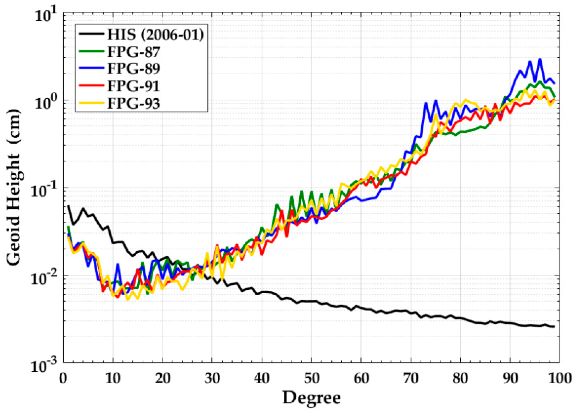
We first evaluate standalone models recovered by different FPG configurations listed in Table 1. The results in January (2006) are demonstrated in Figure 2, while other months show similar results. In Figure 2, the black curve represents the true average HIS signal in January (an integrated signal of terrestrial hydrological water, continental ice-sheets, and the solid earth [24]), while other curves are the degree geoid height errors (DGHE) of different FPG standalone models in this month. Observing signal (in black) and error (in colored) curves, we find that the recovered models are gradually dominated by noises after degree n = 26, which is indicated by the intersection point of signal curve and error curves around degree 26. Among four FPG standalone models, the FPG-91 in general produces smaller errors especially for degrees beyond 60. When looking to low-degree SHC near the intersection point, we find that the retrograde FPGs (FPG-91 and FPG-93) outperform the prograde ones (FPG-89 and FPG-87). The expected degradations of FPG-87 and FPG-93 due to their larger polar gaps compared to FPG-89 and FPG-91, however, is not apparent in Figure 2. This can be explained by denser ground tracks gained by FPG-87 and FPG-93 in the mid and low latitudes, which finally compensate the negative effects caused by large missing polar data, as discussed in [51] (pp. 204–214).

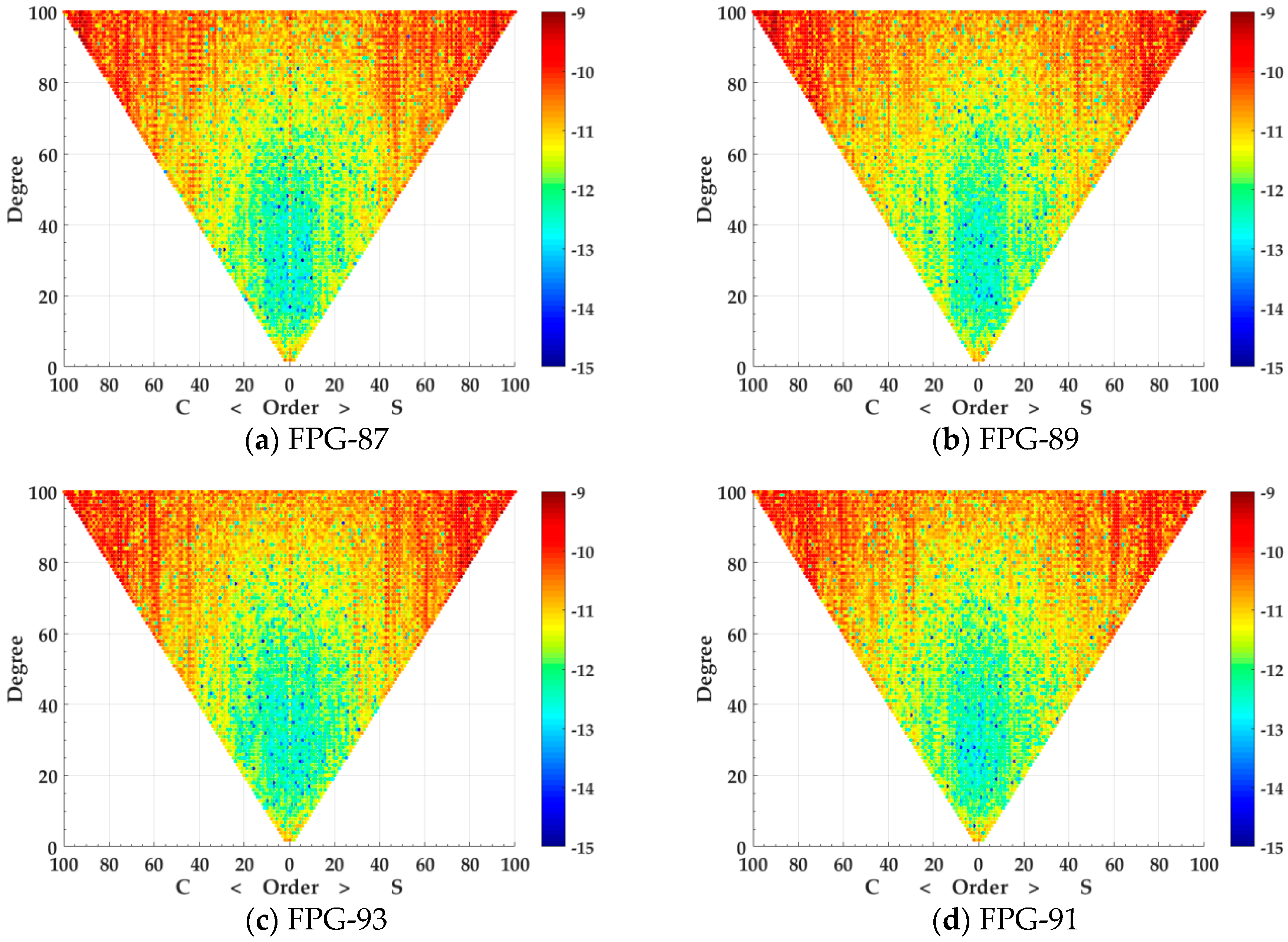
Further comparisons are carried out in terms of absolute SHC differences $(\left|\Delta C_{lm}\right|,\left|\Delta S_{lm}\right|)$ of each degree l and order m, as drawn in Figure 3. Subfigures (a), (b), (c), and (d) stand for results of FPG-87, FPG-89, FPG-93, and FPG-91, respectively. Now we can clearly observe the deficiencies of FPG-87 and FPG-93 in zonal SHC, i.e., $C_{l0}$, estimation, which are demonstrated by larger $\left|\Delta C_{l0}\right|$ values in (a) and (c) compared to that in (b) and (d). Recall the approximate relationship between the polar gap size and the maximum recoverable gravity signal in Section 2.2, the weaknesses of FPG-87 and FPG-93, with 3-degree polar gaps, are expected to become much more pronounced in terms of high-degree, e.g., 180 d/o [11], static gravity model recovery.

3.2. Combined Models of GFO-LRI and FPG

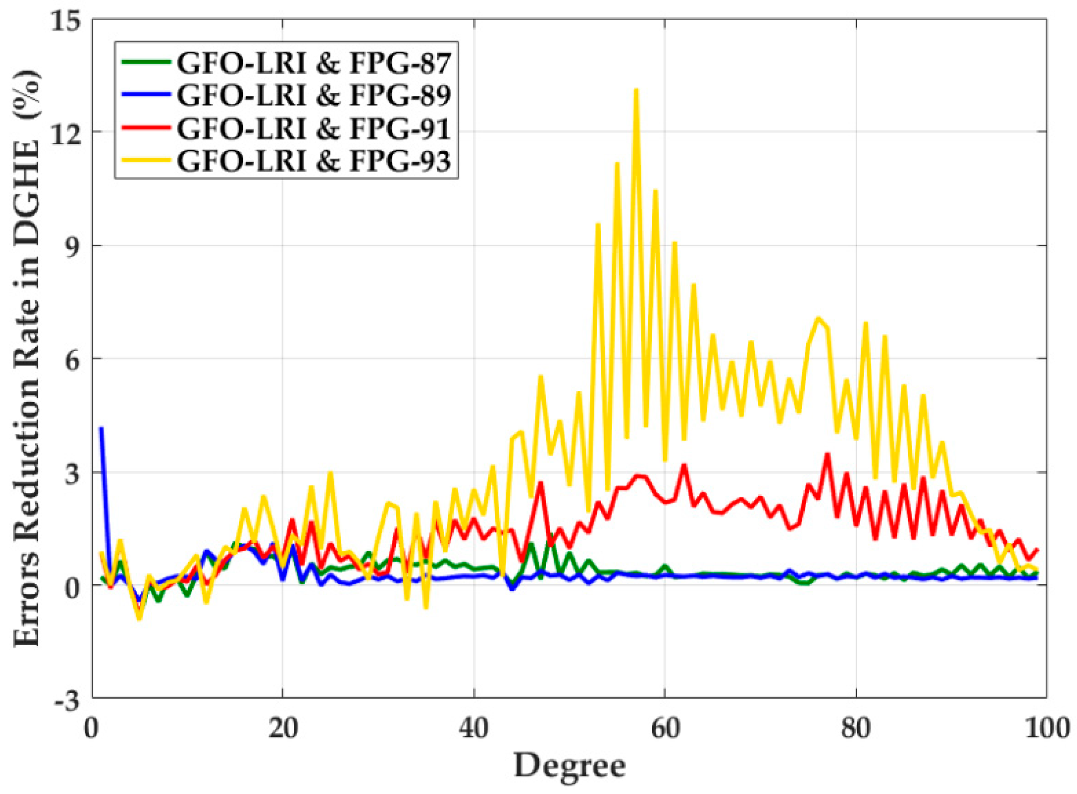
Since GFO carries both LRI and KBR, the combinations between GFO and FPG will be carried out in GFO-LRI & FPG and GFO-KBR & FPG modes respectively. In the GFO-LRI & FPG mode, the information from GFO-LRI will dominate the combined model because it has much larger weight in Equations (9) and (11) than the KBR of FPG, based on Table 3. Therefore, we can expect only minor differences among different GFO-LRI & FPG combined models. Even so, comparisons can still be carried out by calculating the error reduction rate (ERR) of different GFO-LRI & FPG models with respect to the GFO-LRI standalone model. Here, we use the ERR in terms of DGHE, and therefore set $q_i=DGH{E}_{GFO-LRI\&FPG}$ and $q_j=DGH{E}_{GFO-LRI}$ in Equation (16). Figure 4 plots the degree-wise $ER{R}_{GFO-LRI}^{GFO-LRI\&FPG}(DGHE)$ for all four GFO-LRI & FPG models, which can be regarded as contributions of adding different FPGs’ information to the GFO-LRI data.

As expected, the contributions are not significant. Among four combined models, GFO-LRI & FPG-93 has the largest ERR for the majority of SHC, and GFO-LRI & FPG-91 is next after that. Moreover, even with the same polar gap, retrograde FPGs (FPG-91 and FPG-93) outperform the prograde ones (FPG-89 and FPG-87). This can be attributed to the more isotropic integrated system of GFO & retrograde-FPG than GFO & prograde-FPG, as learnt from Bender-type SFF design [37]. More specifically, the orbit inclination differences between the GFO (in prograde orbit) and retrograde FPGs are larger than that in GFO & prograde-FPGs, which enables the GFO & FPG integrated system to observe the gravity signals in a more isotropic sense. However, degradations occur at some very low degrees of the combined models, which is likely due to insufficiently perfect data weighting between GFO-LRI and FPG [61].

3.3. Combined Models of GFO-KBR and FPG

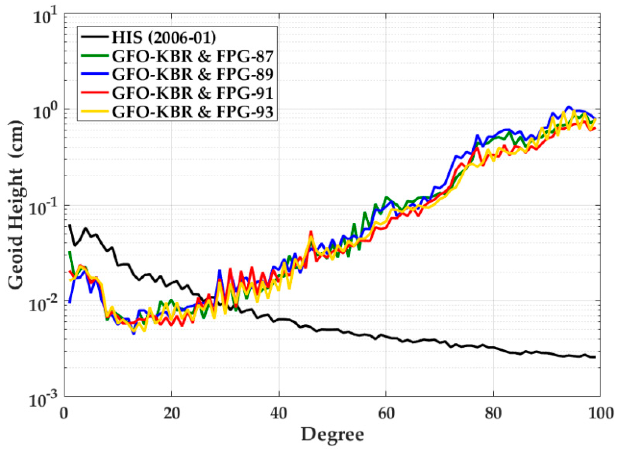
More representative results can be demonstrated by GFO-KBR & FPG combined models. In Figure 5, we plot the true HIS signal (black curve) of January 2006, as well as error curves (in colored) of four GFO-KBR & FPG models in terms of DGHE in this month. Basically, the results are comparable with those in Figure 4, that is, the retrograde FPGs generally outperform prograde ones for their lower DGHE.

Table 4. Error reduction rate (ERR) of different GFO-KBR & FPG combined models with respect to the GFO-KBR standalone model in terms of cumulative geoid height error (CGHE) in January 2006

Degree	GFO-KBR & FPG-87	GFO-KBR & FPG-89	GFO-KBR & FPG-91	GFO-KBR & FPG-93
25	−3.6%	16.7%	7.9%	7.9%
50	17.5%	15.1%	14.6%	16.7%
75	31.1%	16.7%	33.6%	41.6%
100	28.0%	14.7%	39.5%	31.7%

records the ERR of GFO-KBR & FPG combined models with respect to the GFO-KBR standalone model in terms of cumulative geoid height error (CGHE) in Equation (13), which is calculated by setting $q_i=CGH{E}_{GFO-KBR\&FPG}$ and $q_j=CGH{E}_{GFO-KBR}$ in Equation (16). It shows that the retrograde FPGs start highlighting their advantages after degree 50.

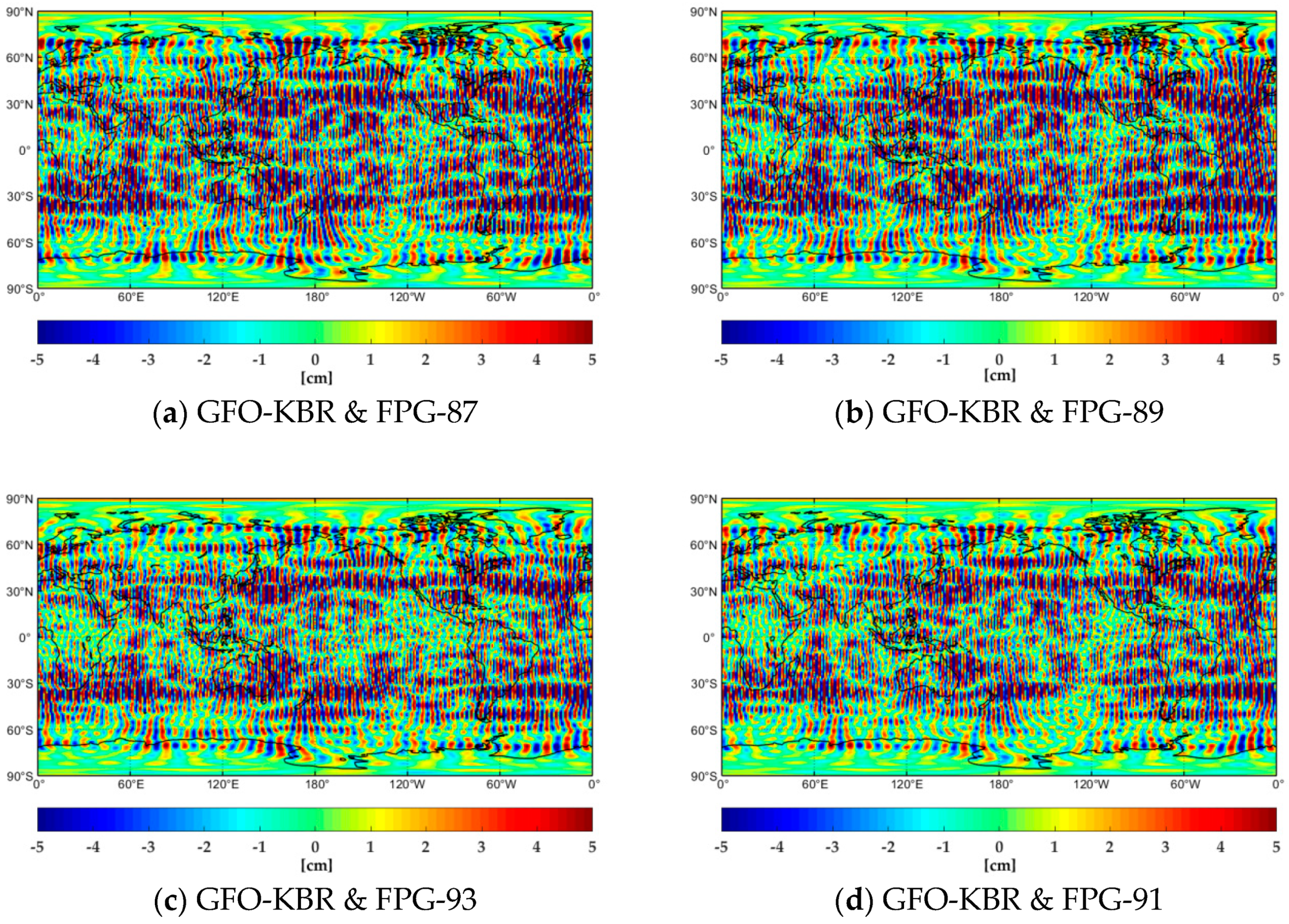
To observe the error patterns in spatial domain, we draw the global spatial differences plots (SDP), introduced in Section 2.4, of above four GFO-KBR & FPG combined models. As shown in Figure 6, obviously fewer stripes can be found in the retrograde-orbit based GFO-KBR & FPG combined models, comparing subfigure (a) GFO-KBR & FPG-87 with (c) GFO-KBR & FPG-93 or (b) GFO-KBR & FPG-89 with (d) GFO-KBR & FPG-91. These typical north-south stripes are, to a large extent, the product of temporal aliasing errors, which are caused by errors in both ocean tide model and Atmosphere and Ocean De-Aliasing (AOD) product [25,26]. It seems that the retrograde FPGs, in combination with GFO, are more effective on reducing the temporal aliasing errors than prograde ones, especially in low-latitude areas within $({30}^{\circ }S,{30}^{\circ }N)$. However, only marginal improvement can be observed over high-latitude regions in Figure 6.

3.4. One-Year GFO-combined Model Series of FPG-89 and FPG-91

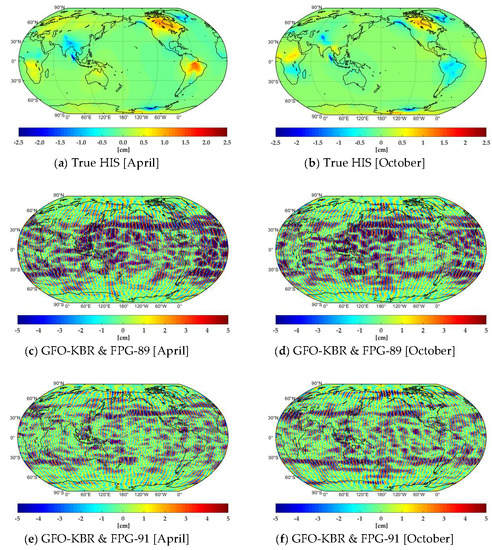
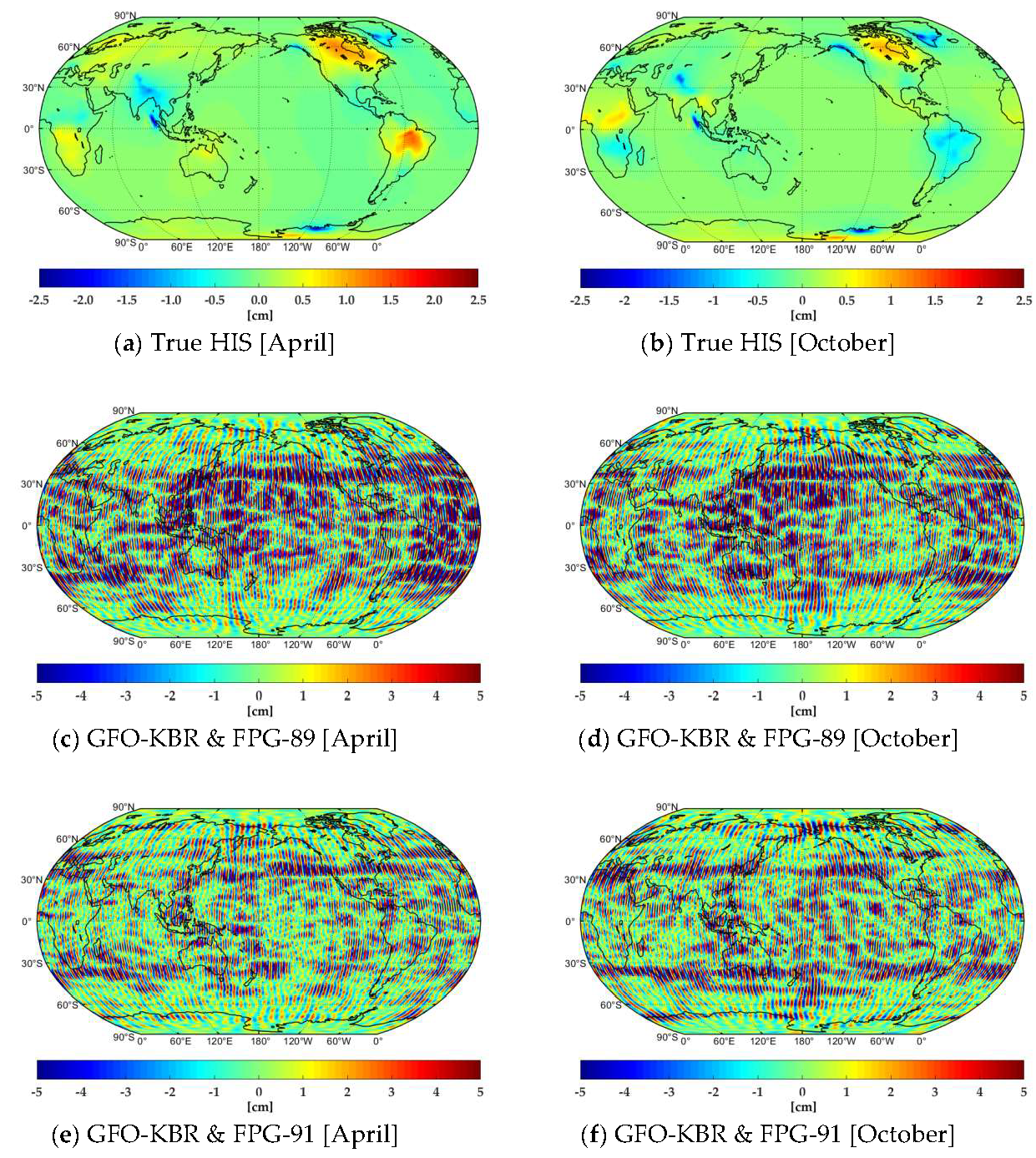
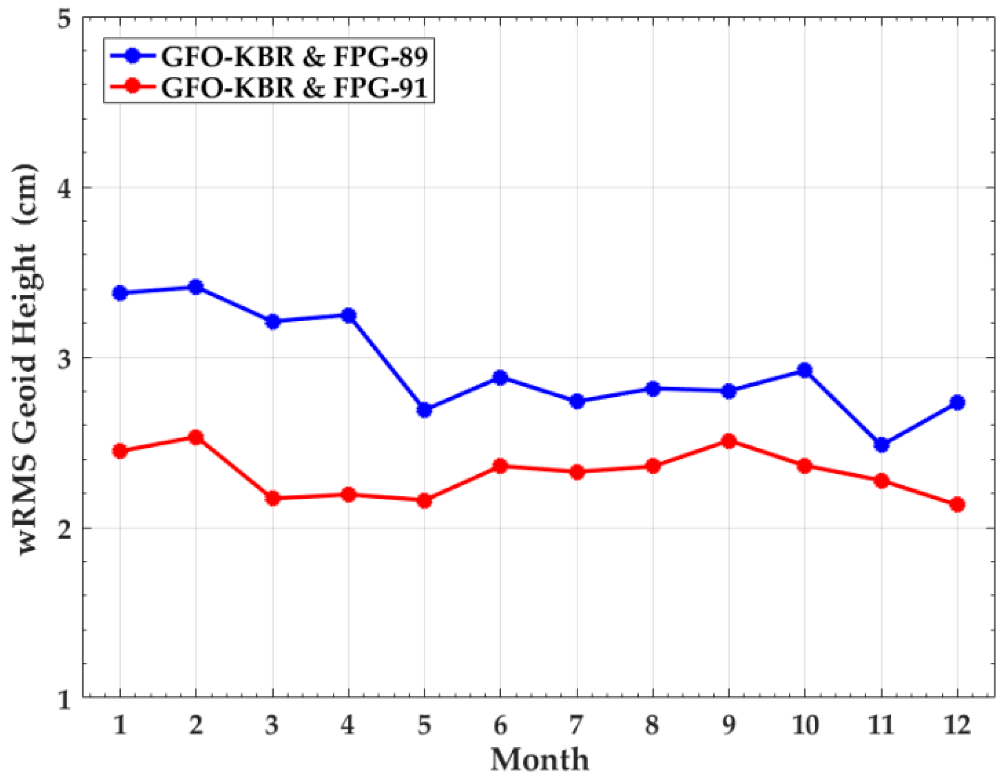
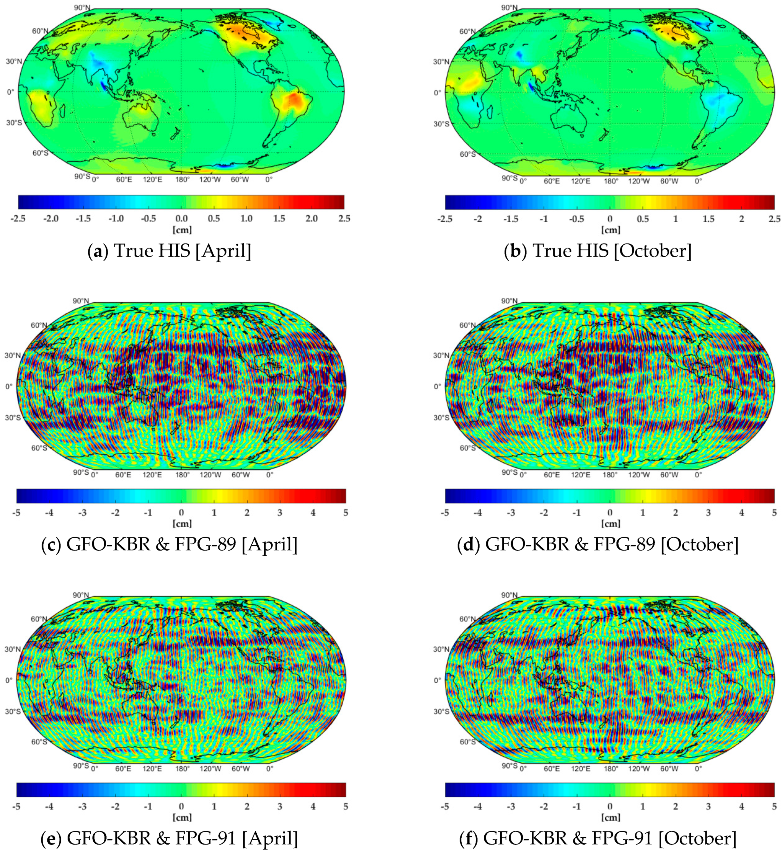
In view of FPG-87 and FPG-93′s deficiencies in zonal SHC determination, we therefore choose FPG-89 and FPG-91 in further GFO-joint gravity model recovery for the entire year 2006. We produce 12 monthly GFO-KBR & FPG models for FPG-89 and FPG-91, respectively. Monthly wRMS values of their global SDPs are demonstrated in Figure 7. As expected, GFO-KBR & FPG-91 outperforms the GFO-KBR & FPG-89 for its lower wRMS values over the whole year. Furthermore, we can observe slight variations in wRMS values of GFO-KBR & FPG-91 and GFO-KBR & FPG-89 models from month to month. Therefore, April and October are selected for further illustrations with corresponding results plotted in Figure 8.

On a global scale, results in April and October are plotted in the left and right columns of Figure 8, respectively. Subfigures in the top row represent the spatial signal plots of monthly true HIS signals, which are created the same way as SDP except that the $(\Delta C_{lm},\Delta S_{lm})=({\overline{C}}_{lm}^{HIS},{\overline{S}}_{lm}^{HIS})$ in Equation (14); The middle and bottom rows represent SDPs of GFO-KBR & FPG-89 and GFO-KBR & FPG-91, respectively. As shown, the GFO-KBR & FPG-91 apparently suffers less from the temporal aliasing errors, especially in low- and medium-latitude areas. The error reductions in these areas are beneficial to the scientific study of global water cycle since the world’s major river basins (e.g., the Amazon and Yangtze Rivers), as well as the majority of oceans, are located in the low and medium latitudes.

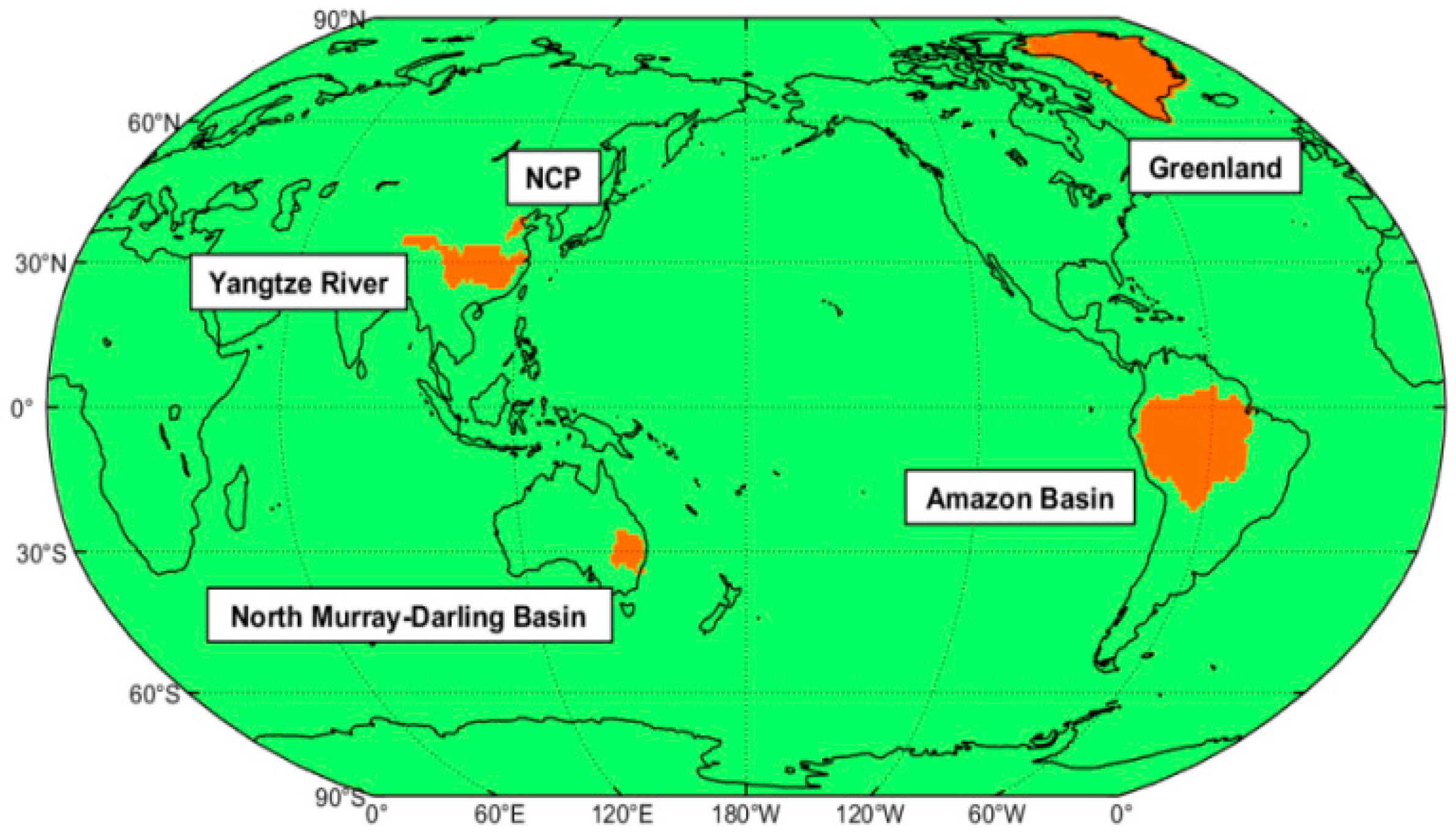
On a regional scale, yearly-average wRMS of GFO-KBR & FPG-89 and GFO-KBR & FPG-91 are respectively calculated based on their regional SDPs. The regions that we select basically represent typical basins in low, medium, and high latitudes as marked in Figure 9. Besides, the ocean and land areas are also separately analyzed. As listed in

Table 5. Yearly-average latitude-weighted root mean squares (wRMS) of regional spatial differences plots (SDP) in GFO-KBR & FPG-89 and GFO-KBR & FPG-91 models. The final column shows the error reduction rate (ERR) of GFO-KBR & FPG-91 with respect to GFO-KBR & FPG-89 in terms of regional wRMS.

Area	wRMS of GFO & FPG-89 (cm)	wRMS of GFO & FPG-91 (cm)	GFO & FPG-91 Error Reduction Rate (%)
Amazon	2.76	1.98	28.3
North Murray–Darling	3.56	2.54	28.7
Yangtze	2.63	2.32	11.8
NCP	3.19	2.89	9.4
Greenland	1.01	1.15	-13.9
Ocean	3.09	2.41	22.0
Land	2.53	2.09	17.4

, the superiority of GFO-KBR & FPG-91 over GFO-KBR & FPG-89 is mainly presented in the low- and medium-latitude regions, including the Amazon basin, North Murray–Darling basin and North China Plain (NCP). The last column of Table 5 shows ERR of GFO-KBR & FPG-91 over GFO-KBR & FPG-89 in terms of regional wRMS by setting $q_i=wRM{S}_{GFO-KBR\&FPG-91}^{\Omega }$ and $q_j=wRM{S}_{GFO-KBR\&FPG-89}^{\Omega }$ in Equation (16). It demonstrates that the GFO-KBR & FPG-91 reduces about 22% errors in ocean and 17% in land areas with respect to GFO-KBR & FPG-89. However, ERR mainly decreases with higher latitude and is even negative in the Greenland. The series of GFO-LRI & FPG-89 and GFO-LRI & FPG-91 models are not demonstrated here because of their indistinctive differences in spatial domain.

4. Discussion

The advantages of GFO & retrograde-FPGs over GFO & prograde-FPGs are believed to be contributed by two aspects. On one hand, since the prograde and retrograde orbits sample the Earth in different directions, combining the two can obtain an integrated system that observes the Earth in a more multi-perspective view. Furthermore, as GFO is flying in a prograde orbit, adding retrograde FPGs (rather than the prograde ones) can make the GFO & FPG integrated system more isotropic [37]. On the other hand, according to the Kaula’s linear perturbation theory [47], the RAANs of prograde and retrograde orbits precess in different directions in the inertial frame. Therefore, when projected into the Earth-fixed frame, the satellite ground tracks of the two evolve with different rates since the Earth rotates eastwards. As such, the signal sampling of the two differs in time domain. Once combined, they contribute to a more homogeneous system for signal sampling in terms of temporal resolution.

Due to the designed polar orbit for polar-type satellites, the low- and medium-latitude areas suffer from much sparser ground tracks than the polar region. The former, however, is just the place where most of temporal aliasing errors appear. Therefore, improved ground tracks in these areas matter much to the final gravity solution, and that is where most of the gains of GFO & FPG-91 come from. However, we also observe the degradation of GFO & FPG-91 at high latitudes such as the Greenland compared with GFO & FPG-89, which is possibly due to the pattern change of GFO & FPG-joint ground tracks at the intersection of prograde FPG-89 and retrograde FPG-91. Similar degradations in the intersection of two Bender-type orbits are also found in [60] (pp. 108–111), which needs further investigations.

5. Conclusions

In this paper, we investigate the orbit configurations for Future Polar-type Gravity missions (FPG) with emphasis on orbit inclination selection via full-scale simulations based on both standalone and joint GFO constellations. Four monthly models in January 2006 under FPG configurations with varying inclinations (87, 89, 91, and 93 degrees) show similar performances except that FPG-87 and FPG-93 suffer from relatively serious deficiencies in the zonal SHC estimation. To improve the GFO-only monthly models, the information from different FPGs are respectively added to them, leading to different GFO & FPG combined models. Among combined models, the retrograde-orbit FPGs (FPG-91 and FPG-93) generally outperform the prograde ones (FPG-89 and FPG-87). The advantages are revealed not only in spectral domain by smaller degree geoid height error (DGHE) and cumulative geoid height error (CGHE), but also in the spatial domain by obvious fewer north–south stripes, especially at low and medium latitudes. More comprehensive investigation is carried out for FPG-89 and FPG-91 by analyzing one-year time series of GFO-KBR joint monthly models, which further highlights the superiority of FPG-91 over FPG-89. Detailed regional analysis shows that improvements mainly reside over those low- and medium-latitude regions. The mechanism behind is explained by more isotropic GFO & FPG observation system that integrates two different orbit types (prograde and retrograde). Based on our study, the FPG configuration with 91-degree inclination is therefore worthy to be recommended for the further orbit design of FPG.

References

- Kusche, J.; Klemann, V.; Sneeuw, N. Mass distribution and mass transport in the earth system: Recent scientific progress due to interdisciplinary research. Surv. Geophys. 2014, 35, 1243–1249. [Google Scholar] [CrossRef]
- Tapley, B.D.; Bettadpur, S.; Ries, J.C.; Thompson, P.F.; Watkins, M.M. GRACE measurements of mass variability in the Earth system. Science 2004, 305, 503–505. [Google Scholar] [CrossRef] [PubMed]
- Colombo, O.L. The Global Mapping of Gravity with Two Satellites; Publications on Geodesy, New Series; Netherlands Geodetic Commission: Delft, Switzerland, 1984. [Google Scholar]
- Jäggi, A.; Hugentobler, U.; Bock, H.; Beutler, G. Precise orbit determination for GRACE using undifferenced or doubly differenced GPS data. Adv. Space Res. 2007, 39, 1612–1619. [Google Scholar] [CrossRef]
- Flury, J.; Bettadpur, S.; Tapley, B.D. Precise accelerometry onboard the GRACE gravity field satellite mission. Adv. Space Res. 2008, 42, 1414–1423. [Google Scholar] [CrossRef]
- Inácio, P.; Ditmar, P.; Klees, R.; Farahani, H.H. Analysis of star camera errors in GRACE data and their impact on monthly gravity field models. J. Geod. 2015, 89, 551–571. [Google Scholar] [CrossRef] [Green Version]
- Dahle, C.; Murböck, M.; Flechtner, F.; GFZ GRACE/GRACE-FO SDS Team. Level-2 GRACE RL06 Products from GFZ. Presented at the GRACE/GRACE-FO Science Team Meeting, Potsdam, Germany, 9 October 2018; Available online: https://presentations.copernicus.org/GSTM-2018-90_presentation.pdf (accessed on 19 January 2019).
- Meyer, U.; Jäggi, A.; Jean, Y.; Beutler, G. AIUB-RL02: An improved time-series of monthly gravity fields from GRACE data. Geophys. J. Int. 2016, 205, 1196–1207. [Google Scholar] [CrossRef]
- Shen, Y.; Chen, Q.; Xu, H. Monthly gravity field solution from GRACE range measurements using modified short arc approach. Geod. Geodyn. 2015, 6, 261–266. [Google Scholar] [CrossRef] [Green Version]
- Chen, Q.; Shen, Y.; Chen, W.; Zhang, X.; Hsu, H. An improved GRACE monthly gravity field solution by modelling the non-conservative acceleration and attitude observation errors. J. Geod. 2016, 90, 503–523. [Google Scholar] [CrossRef]
- Chen, Q.; Shen, Y.; Francis, O.; Chen, W.; Zhang, X.; Hsu, H. Tongji-Grace02s and Tongji-Grace02k: High-Precision Static GRACE-Only Global Earth’s Gravity Field Models Derived by Refined Data Processing Strategies. J. Geophys. Res. Solid Earth 2018, 123, 6111–6137. [Google Scholar] [CrossRef]
- Chen, J.L.; Tapley, B.D.; Save, H.; Tamisiea, M.E.; Bettadpur, S.; Ries, J. Quantification of ocean mass change using GRACE gravity, satellite altimeter and Argo floats observations. J. Geophys. Res. Solid Earth 2018. [Google Scholar] [CrossRef]
- WCRP Global Sea Level Budget Group. Global sea-level budget 1993–present. Earth Syst. Sci. Data 2018, 10, 1551–1590. [Google Scholar] [CrossRef]
- Feng, W.; Zhong, M.; Lemoine, J.M.; Biancale, R.; Hsu, H.T.; Xia, J. Evaluation of groundwater depletion in North China using the Gravity Recovery and Climate Experiment (GRACE) data and ground-based measurements. Water Resour. Res. 2013, 49, 2110–2118. [Google Scholar] [CrossRef] [Green Version]
- Feng, W.; Shum, C.K.; Zhong, M.; Pan, Y. Groundwater Storage Changes in China from Satellite Gravity: An Overview. Remote Sens. 2018, 10, 674. [Google Scholar] [CrossRef]
- Chen, T.; Shen, Y.; Chen, Q. Mass flux solution in the Tibetan Plateau using mascon modeling. Remote Sens. 2016, 8, 439. [Google Scholar] [CrossRef]
- Chen, J.L.; Wilson, C.R.; Tapley, B.D.; Blankenship, D.; Young, D. Antarctic regional ice loss rates from GRACE. Earth Planet. Sci. Lett. 2008, 266, 140–148. [Google Scholar] [CrossRef]
- Flechtner, F.; Neumayer, K.H.; Dahle, C.; Dobslaw, H.; Fagiolini, E.; Raimondo, J.C.; Guntner, A. What Can be Expected from the GRACE-FO Laser Ranging Interferometer for Earth Science Applications? Surv. Geophys. 2016, 37, 453–470. [Google Scholar] [CrossRef]
- Frank, W. GRACE-FO Mission Status and Further Plans. Presented at the GRACE/GRACE-FO Science Team Meeting, Potsdam, Germany, 9 October 2018. [Google Scholar]
- Sheard, B.S.; Heinzel, G.; Danzmann, K.; Shaddock, D.A.; Klipstein, W.M.; Folkner, W.M. Intersatellite laser ranging instrument for the GRACE follow-on mission. J. Geod. 2012, 86, 1083–1095. [Google Scholar] [CrossRef]
- Loomis, B.D.; Nerem, R.S.; Luthcke, S.B. Simulation study of a follow-on gravity mission to GRACE. J. Geod. 2012, 86, 319–335. [Google Scholar] [CrossRef]
- Oppenheim, A.V.; Willsky, A.S.; Nawab, S.H. Signals and Systems, 2nd ed.; Prentice Hall: Upper Saddle River, New Jersey, USA, 1996. [Google Scholar]
- Han, S.C.; Jekeli, C.; Shum, C.K. Time-variable aliasing effects of ocean tides, atmosphere, and continental water mass on monthly mean GRACE gravity field. J. Geophys. Res. Solid Earth 2004, 109. [Google Scholar] [CrossRef] [Green Version]
- Dobslaw, H.; Bergmann-Wolf, I.; Dill, R.; Forootan, E.; Klemann, V.; Kusche, J.; Sasgen, I. The updated ESA Earth System Model for future gravity mission simulation studies. J. Geod. 2015, 89, 505–513. [Google Scholar] [CrossRef]
- Dobslaw, H.; Bergmann-Wolf, I.; Dill, R.; Poropat, L.; Thomas, M.; Dahle, C.; Esselborn, S.; Konig, R.; Flechtner, F. A new high-resolution model of non-tidal atmosphere and ocean mass variability for de-aliasing of satellite gravity observations: AOD1B RL06. Geophys. J. Int. 2017, 211, 263–269. [Google Scholar] [CrossRef] [Green Version]
- Seo, K.W.; Wilson, C.R.; Han, S.C.; Waliser, D.E. Gravity Recovery and Climate Experiment (GRACE) alias error from ocean tides. J. Geophys. Res. Solid Earth 2008, 113. [Google Scholar] [CrossRef] [Green Version]
- Dobslaw, H.; Bergmann-Wolf, I.; Forootan, E.; Dahle, C.; Mayer-Gürr, T.; Kusche, J.; Flechtner, F. Modeling of present-day atmosphere and ocean non-tidal de-aliasing errors for future gravity mission simulations. J. Geod. 2016, 90, 423–436. [Google Scholar] [CrossRef] [Green Version]
- Wahr, J.; Molenaar, M.; Bryan, F. Time variability of the Earth’s gravity field: Hydrological and oceanic effects and their possible detection using GRACE. J. Geophys. Res. Solid Earth 1998, 103, 30205–30229. [Google Scholar] [CrossRef]
- Swenson, S.; Wahr, J. Post-processing removal of correlated errors in GRACE data. Geophys. Res. Lett. 2006, 33. [Google Scholar] [CrossRef] [Green Version]
- Kusche, J.; Schmidt, R.; Petrovic, S.; Rietbroek, R. Decorrelated GRACE time-variable gravity solutions by GFZ, and their validation using a hydrological model. J. Geod. 2009, 83, 903–913. [Google Scholar] [CrossRef] [Green Version]
- Visser, P.N.A.M.; Sneeuw, N.; Reubelt, T.; Losch, M.; van Dam, T. Space-borne gravimetric satellite constellations and ocean tides: Aliasing effects. Geophys. J. Int. 2010, 181, 789–805. [Google Scholar] [CrossRef]
- Wiese, D.N.; Visser, P.; Nerem, R.S. Estimating low resolution gravity fields at short time intervals to reduce temporal aliasing errors. Adv. Space Res. 2011, 48, 1094–1107. [Google Scholar] [CrossRef]
- Daras, I.; Pail, R. Treatment of temporal aliasing effects in the context of next generation satellite gravimetry missions. J. Geophys. Res. Solid Earth 2017, 122, 7343–7362. [Google Scholar] [CrossRef]
- Hauk, M.; Pail, R. Treatment of ocean tide aliasing in the context of a next generation gravity field mission. Geophys. J. Int. 2018, 214, 345–365. [Google Scholar] [CrossRef]
- Wiese, D.N.; Folkner, W.M.; Nerem, R.S. Alternative mission architectures for a gravity recovery satellite mission. J. Geod. 2009, 83, 569–581. [Google Scholar] [CrossRef]
- Bender, P.; Wiese, D.; Nerem, R. A possible dual-GRACE mission with 90 degree and 63 degree inclination orbits. In Proceedings of the International Symposium on Formation Flying, Noordwijk, The Netherlands, 23–25 April 2008; Eur. Space Agency: Noordwijk, The Netherlands, 2008. [Google Scholar]
- Wiese, D.N.; Nerem, R.S.; Lemoine, F.G. Design considerations for a dedicated gravity recovery satellite mission consisting of two pairs of satellites. J. Geod. 2012, 86, 81–98. [Google Scholar] [CrossRef]
- Sneeuw, N.; Sharifi, M.; Keller, W. Gravity Recovery from Formation Flight Missions. In VI Hotine-Marussi Symposium on Theoretical and Computational Geodesy; Xu, P., Liu, J., Dermanis, A., Eds.; Springer: Berlin/Heidelberg, Germany, 2008; Volume 132, pp. 29–34. [Google Scholar]
- Elsaka, B.; Raimondo, J.C.; Brieden, P.; Reubelt, T.; Kusche, J.; Flechtner, F.; Pour, S.I.; Sneeuw, N.; Muller, J. Comparing seven candidate mission configurations for temporal gravity field retrieval through full-scale numerical simulation. J. Geod. 2014, 88, 31–43. [Google Scholar] [CrossRef]
- Cesare, S.; Sechi, G. Next Generation Gravity Mission. In Distributed Space Missions for Earth System Monitoring; D’Errico, M., Ed.; Springer: New York, NY, USA, 2013; Volume 31, pp. 575–598. [Google Scholar]
- Pail, R.; Gruber, T.; Abrykosov, P.; Hauk, M.; Purkhauser, A. Assessment of NGGM Concepts for Sustained Observation of Mass Transport in the Earth System. Presented at the GRACE/GRACE-FO Science Team Meeting, Potsdam, Germany, 10 October 2018; Available online: https://meetingorganizer.copernicus.org/GSTM-2018/GSTM-2018-10.pdf (accessed on 19 January 2019).
- Hsu, H.; Zhong, M.; Feng, W.; Wang, C. Overwiew of activities of Chinese gravity mission. Presented at the International Symposium on Geodesy and Geodynamics (ISGG2018)-Tectonics, Earthquake and Geohazards, Kunming, China, 31 July 2018. [Google Scholar]
- Reigber, C. Gravity field recovery from satellite tracking data. In Theory of Satellite Geodesy and Gravity Field Determination; Sansò, F., Rummel, R., Eds.; Springer: Berlin/Heidelberg, Germany, 1989; Volume 25, pp. 197–234. [Google Scholar]
- Zhou, H.; Luo, Z.; Zhou, Z.; Li, Q.; Zhong, B.; Lu, B.; Hsu, H. Impact of Different Kinematic Empirical Parameters Processing Strategies on Temporal Gravity Field Model Determination. J. Geophys. Res. Solid Earth 2018. [Google Scholar] [CrossRef]
- Guo, X.; Zhao, Q.; Ditmar, P.; Sun, Y.; Liu, J. Improvements in the Monthly Gravity Field Solutions Through Modeling the Colored Noise in the GRACE Data. J. Geophys. Res. Solid Earth 2018, 123, 7040–7054. [Google Scholar] [CrossRef]
- Wang, C.; Xu, H.; Zhong, M.; Feng, W. Monthly gravity field recovery from GRACE orbits and K-band measurements using variational equations approach. Geod. Geodyn. 2015, 6, 253–260. [Google Scholar] [CrossRef] [Green Version]
- Kaula, W.M. Theory of Satellite Geodesy: Applications of Satellites to Geodesy; Dover Publications: New York, NY, USA, 2000. [Google Scholar]
- Chen, Q.; Shen, Y.; Zhang, X.; Hsu, H.; Chen, W.; Ju, X.; Lou, L. Monthly gravity field models derived from GRACE Level 1B data using a modified short-arc approach. J. Geophys. Res. Solid Earth 2015, 120, 1804–1819. [Google Scholar] [CrossRef] [Green Version]
- Shen, Y. Algorithm Characteristics of Dynamic Approach-based Satellite Gravimetry and Its Improvement Proposals. Acta Geod. Cartogr. Sin. 2017, 46, 1308–1315. (In Chinese) [Google Scholar]
- Montenbruck, O.; Gill, E. Satellite Orbits-Models, Methods and Applications; Springer: Berlin/Heidelberg, Germany, 2000. [Google Scholar]
- Kim, J. Simulation Study of a Low-Low Satellite-to-Satellite Tracking Mission. Ph.D. Thesis, The University of Texas, Austin, TX, USA, 2000. [Google Scholar]
- Daras, I. Gravity Field Processing towards Future LL-SST Satellite Missions. Ph.D. Thesis, Technische Universität München, München, Germany, 2016. [Google Scholar]
- Vallado, D. Fundamentals of Astrodynamics and Applications, 4th ed.; Microcosm Press: El Segundo, CA, USA, 2013. [Google Scholar]
- Reigber, C.; Lühr, H.; Schwintzer, P. CHAMP mission status. Adv. Space Res. 2002, 30, 129–134. [Google Scholar] [CrossRef]
- Rummel, R.; Yi, W.; Stummer, C. GOCE gravitational gradiometry. J. Geod. 2011, 85, 777–790. [Google Scholar] [CrossRef]
- Förste, C.; Bruinsma, S.L.; Abrikosov, O.; Lemoine, J.; Marty, J.C.; Flechtner, F.; Balmino, G.; Barthelmes, F.; Biancale, R. EIGEN-6C4 The Latest Combined Global Gravity Field Model Including GOCE Data up to Degree and Order 2190 of GFZ Potsdam and GRGS Toulouse. GFZ Data Services. 2014. Available online: http://icgem.gfz-potsdam.de/getmodel/zip/7fd8fe44aa1518cd79ca84300aef4b41ddb2364aef9e82b7cdaabdb60a9053f1 (accessed on 19 January 2019).
- Savcenko, R.; Bosch, W. EOT11a-Empirical Ocean Tide Model from Multi-Mission Satellite Altimetry; Deutsches Geodätisches Forschungsinstitut (DGFI): München, Germany, 2012. [Google Scholar]
- Darbeheshti, N.; Wegener, H.; Müller, V.; Naeimi, M.; Heinzel, G.; Hewitson, M. Instrument data simulations for GRACE Follow-on: Observation and noise models. Earth Syst. Sci. Data 2017, 9, 833–848. [Google Scholar] [CrossRef]
- Lyard, F.; Lefevre, F.; Letellier, T.; Francis, O. Modelling the global ocean tides: Modern insights from FES2004. Ocean Dyn. 2006, 56, 394–415. [Google Scholar] [CrossRef]
- Wiese, D.N. Optimizing Two Pairs of GRACE-like Satellites for Recovering Temporal Gravity Variations. Ph.D. Theses, University of Colorado, Boulder, CO, USA, 2011. [Google Scholar]
- Meyer, U.; Jean, Y.; Arnold, D.; Jäggi, A.; Kvas, A.; Mayer-Gürr, T.; Lemoine, J.M.; Bourgogne, S.; Dahle, C.; Flechtner, F. The EGSIEM combination service: Final results and further plans. In Proceedings of the EGU General Assembly 2018, Vienna, Austria, 8–13 April 2018; Available online: https://boris.unibe.ch/116268/1/EGU18_EGSIEM-1.pdf (accessed on 19 January 2019).
- Feng, W. GRAMAT: A comprehensive Matlab toolbox for estimating global mass variations from GRACE satellite data. Earth Sci. Inform. 2018, 1–16. [Google Scholar] [CrossRef]
Figure 1.
Processing flow of the forward and the backward simulations.
Figure 2.
True HIS signal and degree geoid height errors (DGHE) of different FPG standalone models in January 2006.
Figure 3.
Absolute spherical harmonic coefficients (SHC) differences of different FPG standalone models in January 2006: (a) FPG-87; (b) FPG-89; (c) FPG-93; (d) FPG-91.
Figure 4.
Error reduction rate (ERR) of different GFO-LRI & FPG combined models with respect to the GFO-LRI standalone model in terms of degree geoid height error (DGHE) in January 2006.
Figure 5.
True HIS signal and degree geoid height errors (DGHE) of different GFO-KBR & FPG combined models in January 2006.
Figure 6.
Global spatial differences plots (SDP) of different GFO-KBR & FPG combined models in January 2006: (a) GFO-KBR & FPG-87; (b) GFO-KBR & FPG-89; (c) GFO-KBR & FPG-93; and (d) GFO-KBR & FPG-91.
Figure 7.
Monthly latitude-weighted root mean square (wRMS) of global spatial differences plots (SDP) for GFO-KBR & FPG-89 and GFO-KBR & FPG-91 in 2006.
Figure 8.
True monthly HIS signal spatial plots and global spatial differences plots (SDP) of GFO-KBR & FPG-89 and GFO-KBR & FPG-91 in April and October 2006: (a) HIS signal in April; (b) HIS signal in October; (c) SDP of GFO-KBR & FPG-89 in April; (d) SDP of GFO-KBR & FPG-89 in October; (e) SDP of GFO-KBR & FPG-91 in April; (f) SDP of GFO-KBR & FPG-91 in October.
Figure 9.
Typical regions selected for GFO & FPG-89 and GFO & FPG-91 models’ comparisons.