1. Introduction
Diurnal variations in sea surface temperature (SST) play an important role in the energy exchange between the ocean and the atmosphere (e.g., [
1,
2]). The key advantage of the infrared radiometers onboard the geostationary satellites is that they enable continuous monitoring of the diurnal cycle in SST (see
Table 1 for list of abbreviations used in the paper). The capabilities of such monitoring have expanded with the launch of a new generation instrument, the Advanced Baseline Imager (ABI) onboard the Geostationary Operational Environmental Satellite (GOES)-16 and -17 (launched on 19 November 2016 and on 1 March 2018, respectively), and the ABI’s twin sensor, the Advanced Himawari Imager (AHI) flown onboard the Japan Himawari-8 and -9 satellites (launched on 7 October 2014 and on 2 November 2016, respectively). Note that Himawari-9 is currently kept on orbit in a storage mode, pending the replacement of Himawari-8 in Japan Meteorological Agency operations, and only occasionally used as a Himawari-8 backup, when the latter is not in service.
The ABI/AHI offers five infrared atmospheric transparency window bands (centered at 3.9, 8.4, 10.3, 11.2, and 12.3 µm) suitable for SST, with high spatial resolution (2 km at nadir, which degrades to ~12 km at satellite view zenith angles, VZA~67°), frequent scans (every 15/10 minutes for ABI/AHI; note that NOAA also considers “Mode 6” for ABI, with a 10 minute refresh rate), and superior radiometric performance [
3,
4,
5]. The NOAA Advanced Clear-Sky Processor for Oceans (ACSPO) system, initially developed to retrieve SST from polar-orbiting sensors, such as NOAA and MetOp AVHRRs; S-NPP and NOAA-20 VIIRS; and Terra and Aqua MODIS [
6], was modified with the launch of Himawari-8 to process data of new generation geostationary sensors [
7,
8,
9]. SSTs retrieved from GOES-16 ABI and Himawari-8 AHI reveal a clear and smooth diurnal cycle. However, accurate quantification of the diurnal cycle in SST requires modifications to the retrieval algorithms currently employed with polar-orbiting sensors.
The magnitude of the diurnal cycle (DCM) is measured as difference between the warmest daytime and the coldest nighttime SSTs. Under the conditions of strong insolation and low wind speed, the local DCM may reach several degrees Kelvin [
10,
11,
12], whereas DCM averaged over larger areas (including the full observed SST domain) is typically estimated from ~0.3–0.5 K [
7,
13]. To correctly measure the DCM, the retrieval algorithm should be able to accurately reproduce both temporal variations and spatial contrasts in the retrieved SST. Furthermore, there may be a substantial difference between the DCM in the upper ~10 μm skin layer of the sea surface (
TSKIN), which forms the thermal infrared emission of the ocean, and
TDEPTH, measured at 0.2–1 m depth by drifting and moored buoys, respectively, and customarily used for training regression SST algorithms [
14,
15]. This calls for algorithms more specifically targeted at
TSKIN versus
TDEPTH retrievals.
Here, we present the SST retrieval algorithms, developed in ACSPO for the ABI and AHI, to specifically improve the estimation of DCM in
TSKIN. The algorithms are evaluated with the emphasis on sensitivity—a scale, in which variations in true SST are reproduced in the retrieved SST,
TS [
16]. It should be noted that the
µ is not a measured quantity. Rather, it is calculated by replacing observed brightness temperatures with simulated derivatives of brightness temperatures in terms of SST in the regression equation and zeroing the terms independent from brightness temperatures. The radiative transfer simulations in ACSPO, including calculations of brightness temperature derivatives, are performed using the Community Radiative Transfer Model (CRTM) [
17]. The input data for the CRTM are the analysis SST, produced by the Canadian Meteorological Center (CMC) [
18], and atmospheric profiles of temperature and humidity from the NCEP Global Forecast System, GFS [
19]. Since the CRTM treats the input SST as
TSKIN, the sensitivity characterizes response of
TS specifically to
TSKIN. We assume that errors of CRTM-based sensitivity calculations are much smaller than typical deficits in sensitivity (~0.1–0.5) for
TS retrieved from geostationary data with conventional algorithms. Optimization of sensitivity (i.e., bringing it as close to 1 as possible) is a prerequisite for accurate DCM estimation, as well as for reproduction of spatial contrasts in
TS. The importance of optimal sensitivity for the analyses of diurnal SST variations was recently stressed in, e.g., [
20].
The most detailed hitherto satellite studies of the diurnal cycle [
11,
12,
13,
21] utilized the multiyear dataset of SST produced from the geostationary Spinning Enhanced Visible and Infrared Imager (SEVIRI) onboard METEOSAT-8 [
22] with the Non-Linear SST (NLSST) algorithm [
23], using two split-window bands at 10.8 and 12 μm. It was shown, however, that the SEVIRI NLSST may include significant regional biases [
24] and that the sensitivity of the NLSST may be suboptimal [
16,
25]. Minimization of regional biases, inherent in the SEVIRI NLSST, has been the objective of developing incremental algorithms, aimed at retrieval of SST increments (i.e., “true minus first guess” SST) from brightness temperature increments (i.e., “observed minus simulated” brightness temperatures). The physical Optimal Estimation method [
26] was applied to the SST retrievals from SEVIRI [
24] and, recently, from Himawari-8 AHI [
27]. In the algorithm [
28], currently used in the reprocessing of SEVIRI data at the EUMETSAT Ocean and Sea Ice Satellite Application Facility [
29], a regression equation with coefficients derived by matching absolute SSTs with absolute brightness temperatures is applied to the retrieval of SST increments from brightness temperature increments. At the early stage of preparations for the GOES-16/17 mission, the concept of the incremental regression was further elaborated [
30] by deriving regression coefficients directly from SST increments matched with brightness temperature increments. Overall, the incremental algorithms were shown capable of reducing regional biases and adjusting the mean sensitivity of retrieved SST [
31,
32]. However, the weakness of the incremental approach is that due to a limited accuracy of the existing radiative transfer models in conjunction with the numerical weather prediction data, the incremental algorithms require correction of biases between observed and simulated brightness temperatures. The latter biases can be estimated for specific geographic regions [
24,
28] or as functions of certain physical variables [
25,
30] by averaging brightness temperature increments over prolonged time periods. As a consequence, the
TS biases are reduced in the statistical sense rather than suppressed in every single image. For this reason, we eventually decided not to implement the incremental method for AHI and ABI within ACSPO in favor of global and piecewise regression algorithms enhanced by using extended sets of radiometric bands and advanced methods of training regression coefficients.
Optimization of the
TS sensitivity has been the most challenging aspect of the adaptation of ACSPO to geostationary data. The processing of Himawari-8 AHI at NOAA started in April 2015 with the initial set of global regression coefficients produced, consistently with the polar-orbiting sensors, by the least-squares fit to
in situ SSTs (
TIS) within the dataset of matchups (MDS) of clear-sky satellite brightness temperatures with
TIS from the NOAA
in situ SST Quality Monitor (
iQuam) system [
33,
34]. However, the sensitivity of the AHI global regression SSTs was found to be much lower than that for the polar-orbiting sensors (VIIRS, AVHRR, and MODIS). The difference in sensitivities between geostationary and polar-orbiting sensors was due to the peculiarities of the observed SST domains.
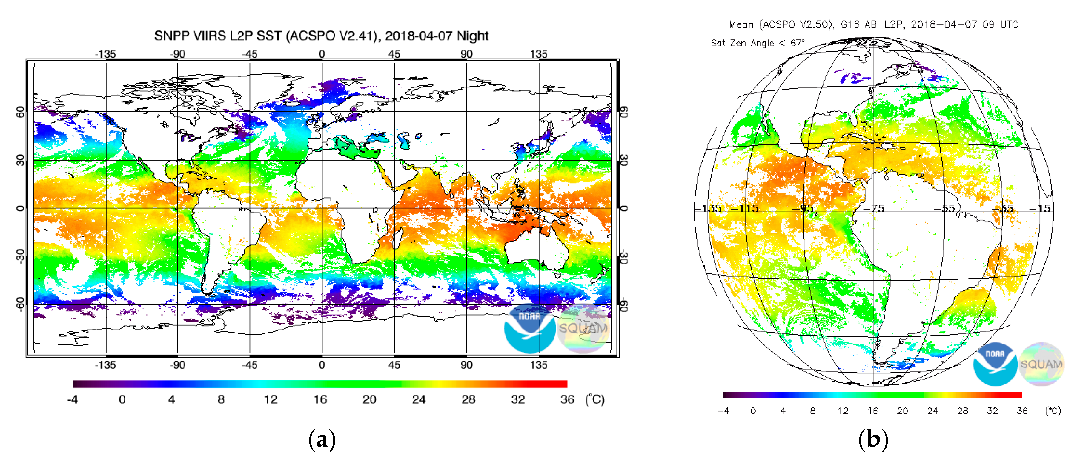
Figure 1 shows the domains observed by the SNPP VIIRS and the GOES-16 ABI. Compared to VIIRS, ABI observes mostly low-latitude regions with relatively warm SSTs, whereas the mid-to-high latitudes with colder SSTs are underrepresented in the ABI images. Moreover, those regions are observed under less favorable conditions (larger VZA and lower spatial resolution). As a result, the MDSs for geostationary sensors are dominated by matchups from low-latitude regions with relatively warm SST, resulting in a narrower distribution of matchups in terms of SST. The global regression coefficients for geostationary satellites, derived from such MDS, are mainly optimized for low-latitude regions, and the mean sensitivity of retrieved SST, averaged over the range of view zenith angles, VZA, 0° ≤ VZA < 67°, is as low as ~0.7, compared to a typical mean sensitivity of ~0.85–0.90 for VIIRS [
25].
In order to increase the sensitivity of the global regression SST, the Constrained Least-Squares Method for training regression coefficients was tested, which fits
TIS under a predefined value of mean sensitivity over the MDS [
8]. This way, the mean sensitivity of AHI global regression SST was raised to ~0.95, which, however, came at the expense of larger regional
TS biases. An alternative method for training the regression coefficients, based on matching nighttime satellite observations with CMC analysis of SST, has been explored after ABI thermal IR data became available in January 2017. Note that the CMC SST is a foundation level 4 product, derived on a daily basis on a 0.1° grid from nighttime satellite SSTs and anchored to
in situ SST measurements [
18]. ACSPO interpolates the gridded CMC SST to every pixel of the sensor. The advantage of the newly developed training method is that, in contrast with matchups with
in situ SST, the number of clear-sky pixels, supplied with CMC SST, is much larger than the number of matchups with
in situ SST, even in near-polar regions. Using the regression coefficients, calculated with the least-squares method from matchups with CMC SST, the mean sensitivity of the global regression SST was raised to ~0.9, without a noticeable increase in regional biases. The next step towards optimization of
TSKIN estimates has been the development of the piecewise regression algorithm, which provides optimal and uniform sensitivity in each SST pixel. In this paper, we compare the performance of the global regression algorithms trained against
in situ and CMC SSTs (GR-IS SST and GR-L4 SST, respectively), and explore the potential of further sensitivity optimization by employing a PWR algorithm, trained against the CMC (PWR-L4).
3. Training Global Regression Algorithms
The dataset of matchups with
in situ SST (MDS-IS), used in this study, includes N = 977,439 matchups of ABI clear-sky observations (both day and night) with high-quality
iQuam drifting and moored buoys. The matchups were collected from April 2017 to March 2018, with a time/space window of 15 min and 10 km, respectively. Every matchup was supplied with simulated brightness temperature derivatives in terms of SST, required for sensitivity calculations, and with GFS data, including wind speed near the sea surface,
V, and total column precipitable water vapor content in the atmosphere,
W. The difficulty of using
in situ SST in the context of
TSKIN retrievals is that
TIS represents
TDEPTH, which may significantly deviate from
TSKIN. The discrepancy between
TSKIN and
TIS reaches the maximum during the daytime under the conditions of strong insolation and low wind speeds near the sea surface [
14,
15]. To minimize the effect of this discrepancy on trained GR-IS SST coefficients, the daytime matchups with
V < 6 m/s were excluded from the training MDS (TMDS-IS). This has reduced the number of matchups within the TMDS-IS to N = 795,877 matchups, or by 18.6%.
The dataset used for training the GR-L4 SST and the PWR-L4 coefficients (TMDS-L4) was composed from nighttime clear-sky ABI L2P SST pixels, supplied with CMC SSTs. Only nighttime data were used because the foundation CMC SST is produced from nighttime SST data (for which the foundation SST is most close to TSKIN) and does not capture the daytime variations in TSKIN. Therefore, using daytime SST pixels for training the GR-L4 SST coefficients would result in additional errors. The TMDS-L4 was formed from 744 ABI images taken every hour from 15 December 2017 to 15 January 2018. A full ABI L2P SST image contains on average 3.2 × 10⁶ clear-sky pixels, with approximately half of those being nighttime. The total number of nighttime pixels within the TMDS-L4 reaches 1.19 × 10⁹, which is 1.5 × 10³ times larger than the number of matchups within the TMDS-IS.
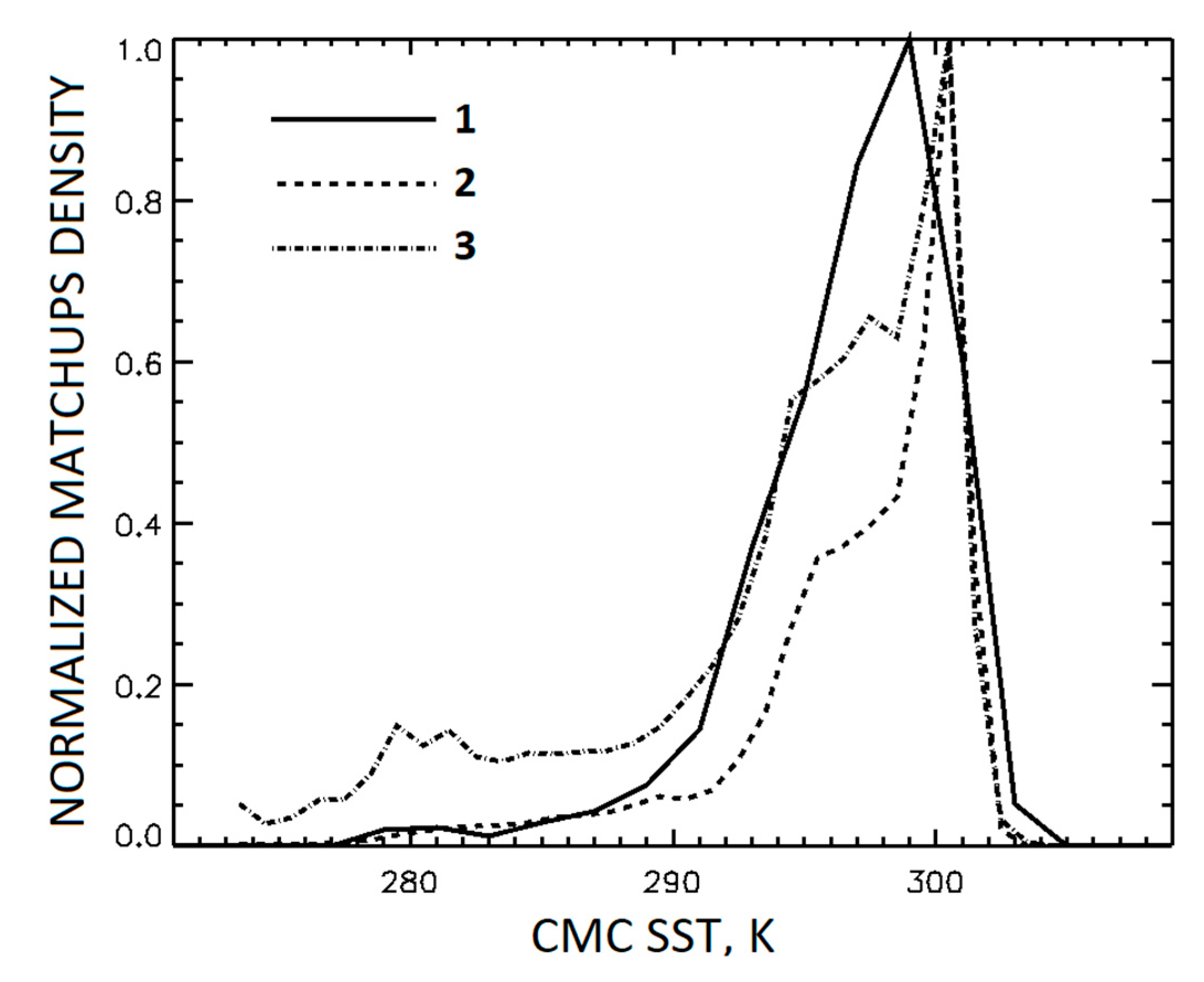
The large number of pixels within the TMDS-L4 allows improvement to the performance of the GR-L4 SST compared with the GR-IS SST. Curves 1 and 2 in
Figure 2 show the normalized histograms of matchups within TMDS-IS and TMDS-L4, as functions of CMC SST. For both these distributions the majority of matchups is concentrated at warm SSTs > 285 K, and the histogram for TMDS-L4 is even narrower than for TMDS-IS. The advantage of TMDS-L4, however, is that the absolute number of clear-sky pixels in the high-latitude regions is much larger than the number of matchups with
in situ SST. It is possible, therefore, to improve the performance of the GR-L4 SST by accounting for the pixels from the under-represented regions with larger weights. When training the GR-L4 SST and the PWR-L4 SST algorithms, the weights of the pixels within each 5° × 5° lat/lon box were selected in inverse proportion to total numbers of clear-sky pixels within the box. The curve 3 in
Figure 2 shows the modified normalized histogram, which accounts for weights of the clear-sky pixels within the TMDS-L4. The weighting expands the histogram and increases the contribution of cold pixels to the overall statistics.
The GR-IS SST algorithm was trained with the least-squares method, which minimizes the global standard deviation of TS from TIS. The GR-L4 SST was trained by minimization of the weighted standard deviation of Ts from TS0. After training, the offsets of the GR-IS and GR-L4 equations were adjusted to zero bias between retrieved SSTs and TIS averaged over matchups within the TMDS-IS from 12 am to 7 am local solar time.
4. The PWR-L4 SST Algorithm
As will be shown in
Section 5, the GR-L4 SST increases the sensitivity compared with the GR-IS SST but leaves it suboptimal and non-uniform. The goal of the PWR-L4 SST is to further optimize the sensitivity in every pixel. The algorithm is constructed and performs as follows.
During off-line training, the vector of GR-L4 coefficients,
CGR-L4, is derived from TMDS-L4, as described in
Section 3, and the GR-L4 sensitivity,
µGR-L4 =
CGR-L4TK, is calculated for all pixels (
K is defined in Equation (4)). The whole TMDS-L4 is subdivided into 9 subsets in terms of
µGR-L4:
Here,
i is the number of the subset. The first guess of the PWR-L4 coefficients for the
ith subset,
C1i, is derived with the Constrained Least-Squares Method [
8], by minimization of the weighted standard deviation of
TS −
TS0 under the constraint on the mean sensitivity: (
C1i)
T<K> = 1, <*> denotes averaging over the pixels belonging to a given TMDS-L4 subset. The offsets
ai are defined in order to zero the bias of
TS with respect to
in situ SST over the subset of TMDS-IS, which includes matchups with the corresponding sensitivities, taken from 0 to 7 am of the local solar time:
<<*>> in Equation (6) denotes averaging over a given TMDS-IS subset. Similarly, the particular offsets of the GR-L4 SST equations for the
ith subset,
bi, are defined as
The values of C1i, a1i, bi and mean values of the GR-L4 SST sensitivities, µi = <µGR-L4>, I = 1, 2, …, 9, are stored in the look-up table.
During processing, every SST pixel is attributed to a specific subset depending on a pixel value of µGR-L4 and the PWR-L4 SST equation for this pixel is modified with two sequential iterations. The second iteration of the PWR-L4 coefficients and the offsets, {a2, C2} ensures their continuity in terms of µGR-L4:
If
µi <
µGR-L4 ≤
µi + 1, I = 1, 2, …, 8:
The third iteration brings the PWR-L4 sensitivity exactly to 1 by extrapolation/interpolation between the second iteration of the PWR-L4 sensitivities,
µ2=
C2TK, and
µGR-L4:
Considering that
µGR-L4 =
CGR-L4TK, the sensitivity of the
TS, produced with coefficients
C3 from Equation (11),
C3TK ≡ 1. Finally, the PWR-L4 SST is calculated as
5. Validation Against In Situ SST
In this Section, the explored algorithms are evaluated and compared using matchups from the MDS-IS. In order to minimize the contribution of the discrepancies between
TIS and
TSKIN to the validation statistics, biases and standard deviations of
TS – TIS, as well as mean sensitivities are calculated from TMDS-IS, which, as described in
Section 3, excludes daytime matchups with GFS wind speeds
V < 6 m/s. In contrast, the DCM estimates are produced from the full MDS-IS, taking into account both daytime and nighttime matchups at all wind speeds. It should be noted that since the TMDS-IS was used for training the GR-IS coefficients, it can be viewed as a dependent MDS in terms of validating the GR-IS SST. However, it is independent in terms of validating the GR-L4 and the PWR-L4 SSTs. This suggests that the conditions of the comparison are more favorable for the GR-IS SST than for two other algorithms.
Absorption by the atmospheric water vapor is a major factor, modifying the responses of brightness temperatures, observed in the atmospheric transmission window, to variations in SST (e.g., [
37,
38]). The performance of the regression algorithms (including sensitivity) usually degrades with the increase of the water vapor content along the sensor’s slant line of sight, STPW =
W × sec (θ) [
25]. It is important, therefore, to determine the ranges of STPW, suitable for retrieval of
TSKIN with the explored algorithms. The statistical factor which should also be considered when comparing different training techniques is the distribution of matchups within the training MDS.
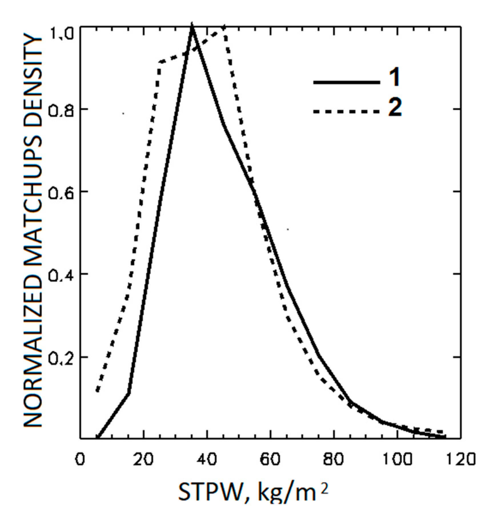
Figure 3 shows the normalized histograms of matchups within TMDS-IS and TMDS-L4 as functions of STPW. The histogram for TMDS-L4 accounts for weighting the pixels during training the GR-L4 and PWR-L4 coefficients, as described in
Section 3. The latter histogram shows wider maximum and increased contribution of matchups with STPW < 30 kg/m
2, typical for mid- and high latitudes.
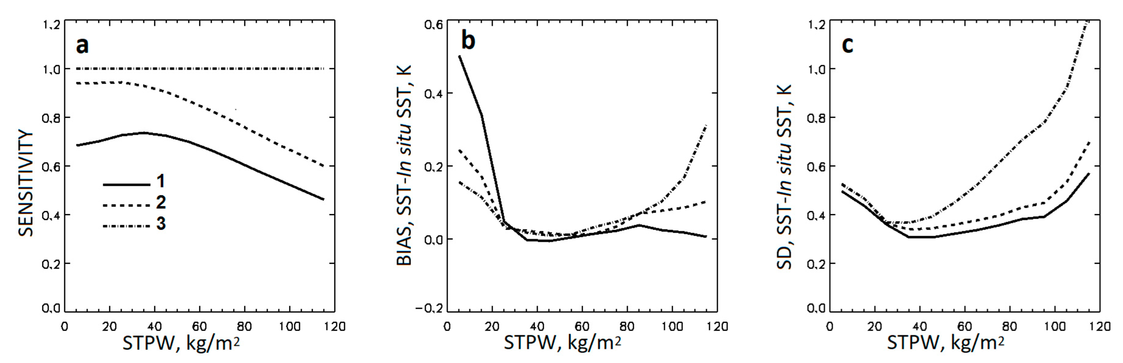
Figure 4 shows mean sensitivities, biases, and standard deviations as functions of STPW. All algorithms perform best near the maxima of the corresponding matchups’ distributions at 30 < STPW < 50 kg/m
2, rather than at the minimum of STPW, as one could expect from physical considerations. At smaller STPWs the biases and the standard deviations increase for all three algorithms, and the sensitivities for the GR-IS and GR-L4 SSTs reduce due to reduced relative numbers of corresponding matchups within the training MDSs. At larger STPWs, the statistics are affected by a combination of increasing atmospheric absorption and decreasing relative numbers of matchups. In
Figure 4a, the GR-IS SST sensitivity is as low as 0.75 at its maximum near STPW = 30 kg/m
2 and reduces to 0.40 at STPW = 130 kg/m
2. The sensitivity of the GR-L4 SST reaches 0.95 at STPW = 20 kg/m
2 but reduces to 0.56 at STPW = 130 kg/m
2. The sensitivity of the PWR-L4 SST, by design, remains constant and optimal at all STPWs. In
Figure 4b, the biases for all three SSTs do not exceed 0.1 K within the range 20 < STPW < 80 kg/m
2. At STPW < 20 kg/m
2, the large bias in the GR-IS SST is caused by the insufficient number of matchups within the TMDS-IS, whereas the biases in the GR-L4 SST and, especially, PWR-L4 SST increase to a lesser extent. In
Figure 4c, the standard deviations for all three SSTs increase with STPW > 40 kg/m
2, consistently with the sensitivities in
Figure 4a. Thus, we conclude that the sensitivity of the GR-L4 SST is suboptimal for estimations of the DCM in
TSKIN within the whole range of STPW. The DCM estimates from GR-L4 SST may be appropriate at STPW < 60 kg/m
2 but become suboptimal at larger STPWs because of degraded sensitivity. On the other hand, the
TSKIN retrievals and DCM estimates, made from the PWR-L4 SST, may be inefficient at large STPWs due to degraded accuracy and precision. Considering the above, we restrict the range of STPW for
TSKIN retrieval with STPW < 100 kg/m
2. This excludes nearly 0.6% of the MDS-IS and TMDS-IS matchups from the further analysis.
Figure 5a illustrates the effect of sensitivity on the reproduction of the diurnal cycle in
TS with three algorithms by showing the hourly biases of
TS −
TS0 as functions of local solar time. The latter biases were estimated from the MDS-IS, using 970,371 daytime and nighttime matchups at all wind speeds and with STPW < 100 kg/m
2.
Figure 5a also shows the hourly biases in
TIS −
TS0. The diurnal cycles are well expressed in all three retrieved SST as well as in
Tis, although with substantially different DCMs. The maxima and the minima in
TIS −
TS0 take place later than in
TS −
TS0, consistent with the fact that the “skin” layer cools down and warms up faster than the “depth” layer, at which the
in situ SST is measured.
Figure 5b shows the hourly biases in
TS −
TIS. The biases in
TS −
TIS in
Figure 5b are smaller than in
TS −
TS0 in
Figure 5a. One can also notice that the maxima and the minima of biases in
TS − TIS shift to a later time when the mean sensitivity of an SST product increases.
Table 2 summarizes mean sensitivities, SDs, and DCMs, estimated from the corresponding subsets of matchups. Overall, training the GR coefficients against CMC increases all three statistics compared with training against
in situ SST and so does the adjustment of sensitivity in the PWR-L4 SST. More specifically, the 25% increase in mean sensitivity between the GR-IS SST and the GR-L4 SST results in comparable (22%) increase in DCM and disproportionally small (9%) increase in SD. On the other hand, the 11% increase in mean sensitivity between the GR-L4 and PWR-L4 SSTs causes a 12% increase in DCM and a larger (14%) increase in SD. This result, consistent with
Figure 4b,c, suggests that estimation of the PWR-L4 coefficients with the CLS method may cause amplification of regional biases compared with those in the GR-L4 SST.
6. Processing GOES-16 ABI Data
The three algorithms have been implemented within the experimental version of ACSPO and tested on GOES-16 ABI data from 1 March–31 March 2018. Since the operational ACSPO Clear-Sky mask [
39] uses retrieved SST as one of the clear-sky predictors, the clear-sky SST domains may be somewhat different for different retrieval algorithms. To ensure the comparison of the algorithms on the same domain, a single clear-sky mask, generated with the GR-L4 SST, was consistently employed with all three algorithms.
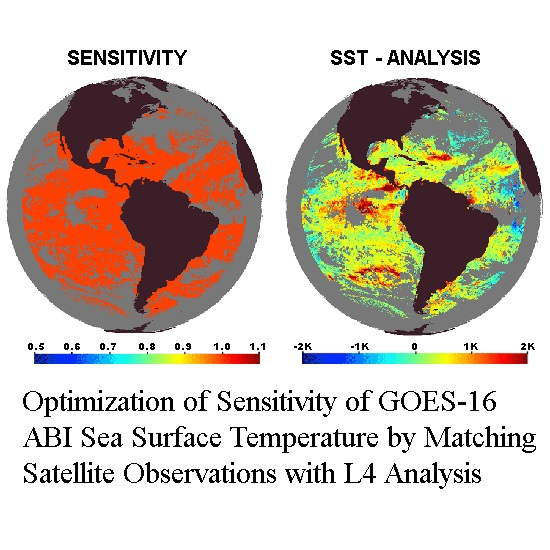
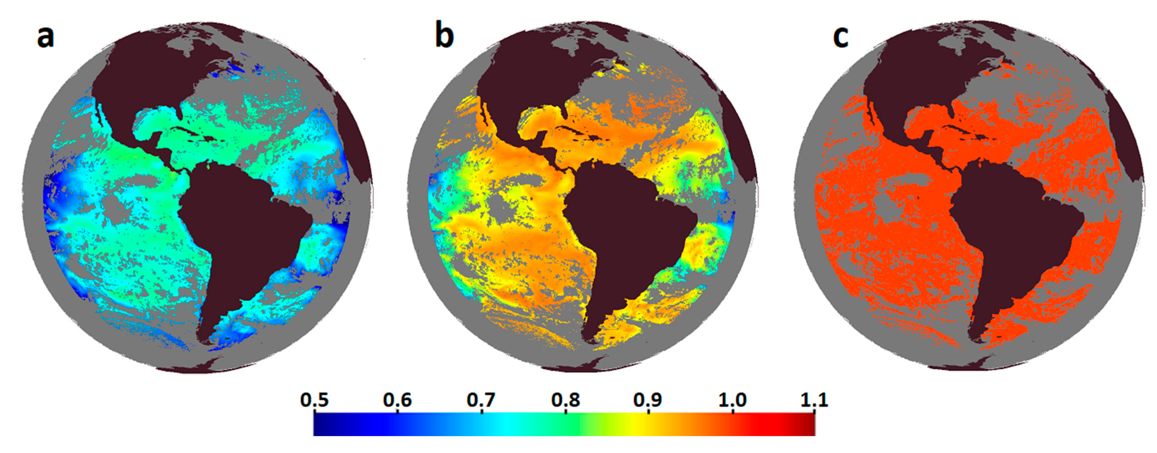
Figure 6 shows geographical distributions of sensitivities for three SSTs retrieved from the ABI data on 1 March 2018 at 20:00 UTC (close to the maximum of the diurnal warming signal within the GOES-16 ABI domain).
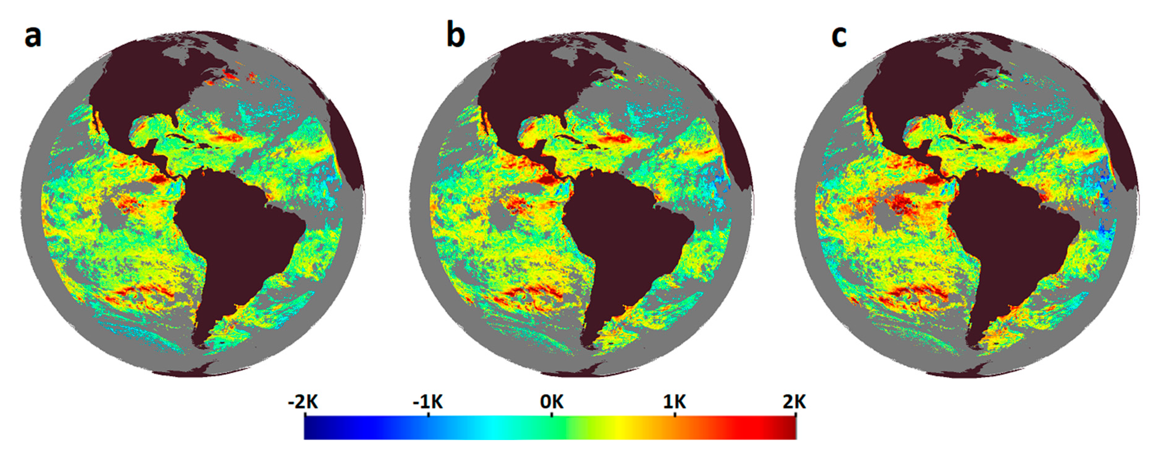
Figure 7 shows deviations of the retrieved SSTs from CMC SST for the same ABI data. The statistics of sensitivities for the images in
Figure 6 and of
TS − TS0 for the images in
Figure 7 are given in
Table 3. In
Figure 6, the GR-IS SST has the lowest and variable sensitivity. The GR-L4 SST sensitivity is higher than for the GR-IS SST and is also variable. For both the GR-IS SST and the GR-L4 SST, the sensitivities are especially low in the low latitudes at large VZAs, due to large atmospheric absorption along the line of sight, consistent with the behavior of sensitivities at large STPWs in
Figure 4a. The GR-IS sensitivity is also reduced in the near-polar zones, which are poorly represented within TMDS-IS. The PWR-L4 SST, by design, provides optimal and uniform sensitivity,
µ ≡ 1, over the full SST domain.
Overall, the three products show similar diurnal warming patterns, but with different amplitudes. The exceptions are unrealistically warm biases in the GR-IS SST in the North Atlantic Ocean and smaller biases at the south-western edge of the image, which are not reproduced (or are less noticeable) in the two other SSTs. Differences between the GR-L4 and the PWR-L4 SSTs are more noticeable in regions with relatively low GR-L4 sensitivities: for instance, the PWR-L4 SST is warmer in the Equatorial Pacific Ocean and in the Southern Atlantic and colder in the Equatorial Atlantic at the eastern edge of the image, due to the effect of the Saharan dust outbreak.
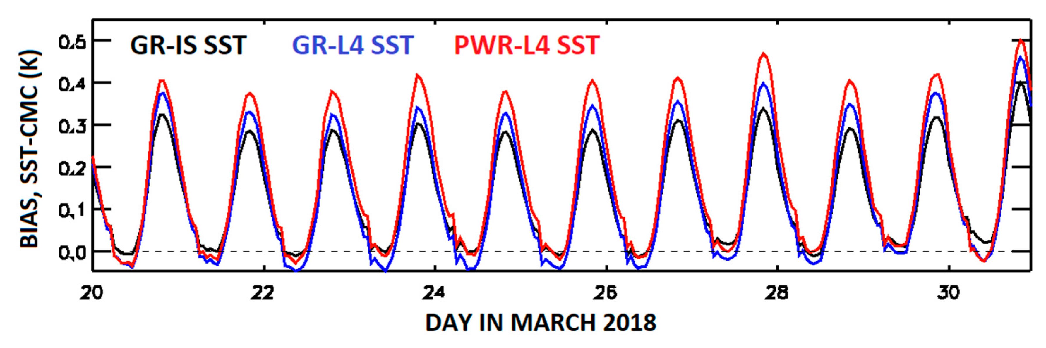
Figure 8 shows the time series of biases in retrieved SST–CMC SST for 20–30 March 2018. The DCMs increase from GR-IS to GR-L4 and to PWR-L4 SST.
Table 4 shows the mean sensitivities and DCMs for three algorithms averaged over the month from 1–31 March 2018. The DCMs in
Table 4 are roughly proportional to mean sensitivities.
Figure 9 shows the mean values of DCMs, averaged from 1–31 March 2018, as functions of STPW. The corresponding dependencies for sensitivities are similar to those produced from matchups and shown in
Figure 4a. The unrealistically large DCM in the GR-IS SST at STPW < 10 kg/m
2 confirms that this algorithm is inefficient at small STPWs. Other than that, the changes in DCM between the algorithms are consistent with the differences in the sensitivities. The difference between the DCMs estimated from the GR-IS SST and the GR-L4 SST is the largest at STPW < 60 kg/m
2. In contrast, the difference between the DCMs for GR-L4 SST and PWR-L4 SST is small at 10 < STPW < 40 kg/m
2 and increases with STPW growing over 40 kg/m
2 due to increased difference in sensitivities. Assuming that that the maximum of the clear-sky pixels distribution takes place at 30 < STPW < 50 kg/m
2, consistent with the maximum of the distribution of matchups in
Figure 3, the adjustment of the DCM estimates in the PWR-L4 SST at larger STPWs may essentially exceed the mean difference between the average DCM values for GR-L4 and PWR-L4 SSTs shown in
Table 4.
8. Summary and Conclusions
The sensitivity of retrieved SST to TSKIN is a characteristic of an SST retrieval algorithm, which determines the reproduction of true spatial and temporal SST variations in retrieved SST. The sensitivity directly affects the magnitude of diurnal SST variations, estimated from geostationary sensors, and, therefore, it is of particular importance for the quantitative monitoring of the diurnal cycle in SST. The sensitivity may substantially vary for different SST algorithms depending on the algorithm’s design and the method of training regression coefficients. Optimization of the sensitivity at the stage of algorithm development, i.e., bringing it as close to 1 as possible, is a prerequisite for accurate estimation of the magnitude of the diurnal cycle in SST.
The conventional method of training regression SST algorithms, developed earlier for polar-orbiting sensors, implies matching satellite observations with drifting and moored buoys. We have found this method suboptimal for geostationary sensors because it provides the sensitivity to TSKIN, averaged over the full observed SST domain, as low as ~0.7. As an alternative to training against in situ SST, we have developed the method of training by matching nighttime clear-sky satellite observations with analysis L4 SST in conjunction with weighting the clear-sky pixels in the inverse proportion to their spatial density. With the newly developed training method, the average sensitivity of the global regression SST for GOES-16 ABI has been increased from ~0.7 to ~0.9 without noticeable increase of regional biases. However, even with this improved training method, the sensitivity of the global regression SST remains variable and suboptimal.
The ultimate optimization of sensitivity has been further accomplished with the development of the piecewise regression algorithm, which exploits the segmentation of the SST domain in terms of sensitivity of the global regression SST, trained against L4 CMC SST, and calculates the coefficients for each segment under the mean sensitivity constrained at 1. While the improvement in sensitivity of the global regression algorithm due to training against L4 SST increases the magnitude of the diurnal cycle in SST almost uniformly over the ABI SST domain, the piecewise regression SST algorithm further increases the magnitude of the diurnal cycle in the areas with larger atmospheric absorptions, in which the sensitivity of the global regression SST is relatively low.
The global regression algorithm with coefficients, trained on CMC SST, has been implemented as a primary ACSPO algorithm for GOES-16/17 ABI and Himawari-8 AHI, starting with the operational ACSPO version 2.60. The PWR “skin” algorithm has been implemented as an experimental algorithm in ACSPO version 2.61 for internal testing. The future work will be focused on detailed validation of TSKIN retrievals from the aforementioned satellites and optimization of SST retrieval algorithms, including minimization of the diurnal variability of biases in retrieved SST.


