Cropland Mapping Using Fusion of Multi-Sensor Data in a Complex Urban/Peri-Urban Area
by
 , and
, and
Eunice Nduati
1,* ,
,
Yuki Sofue
1,
Akbar Matniyaz
1,
Jong Geol Park
2,
Wei Yang
1,3 and
Akihiko Kondoh
1,3 1
Department of Earth Sciences, Chiba University, 1-33, Yayoi-cho, Inage-ku, Chiba-shi, Chiba 263-8522, Japan
2
Department of Informatics, Tokyo University of Information Sciences, 4-1 Onaridai, Wakaba-ku, Chiba 265-8501, Japan
3
Center for Environmental Remote Sensing, Chiba University, 1-33 Yayoi-cho, Inage-ku, Chiba-shi 263-8522, Japan
*
Author to whom correspondence should be addressed.
Remote Sens. 2019, 11(2), 207; https://0-doi-org.brum.beds.ac.uk/10.3390/rs11020207
Submission received: 19 November 2018
/
Revised: 13 January 2019
/
Accepted: 13 January 2019
/
Published: 21 January 2019
(This article belongs to the Special Issue High Resolution Image Time Series for Novel Agricultural Applications)
Abstract
:Urban and Peri-urban Agriculture (UPA) has recently come into sharp focus as a valuable source of food for urban populations. High population density and competing land use demands lend a spatiotemporally dynamic and heterogeneous nature to urban and peri-urban croplands. For the provision of information to stakeholders in agriculture and urban planning and management, it is necessary to characterize UPA by means of regular mapping. In this study, partially cloudy, intermittent moderate resolution Landsat images were acquired for an area adjacent to the Tokyo Metropolis, and their Normalized Difference Vegetation Index (NDVI) was computed. Daily MODIS 250 m NDVI and intermittent Landsat NDVI images were then fused, to generate a high temporal frequency synthetic NDVI data set. The identification and distinction of upland croplands from other classes (including paddy rice fields), within the year, was evaluated on the temporally dense synthetic NDVI image time-series, using Random Forest classification. An overall classification accuracy of 91.7% was achieved, with user’s and producer’s accuracies of 86.4% and 79.8%, respectively, for the cropland class. Cropping patterns were also estimated, and classification of peanut cultivation based on post-harvest practices was assessed. Image spatiotemporal fusion provides a means for frequent mapping and continuous monitoring of complex UPA in a dynamic landscape.
1. Introduction
Uncertain climatic conditions, high population growth, commodity price fluctuation, urbanization, and allocation of agricultural produce to non-food consumption uses all threaten global and regional food security [1,2,3,4,5,6]. Eigenbrod and Gruda [3] highlighted the need for analysis of crop area and production that takes into account changing demographics vis-a-vis urbanization. In a global assessment of urban and peri-urban agriculture, Thebo et al. [7] noted that, despite the increasing significance of urban and peri-urban agriculture (UPA), it remains poorly quantified. Common to UPA-related studies is the need for spatially explicit cropland data [7,8,9]. Numerous studies and projects on cropland and crop-type mapping have been conducted to provide information about crop distribution, crop types, and cropping frequency, at global, regional, and local scales [10,11,12,13,14,15,16,17,18,19,20,21,22]. In particular, remote sensing is a critical source of data for agricultural mapping and monitoring, since it offers synoptic earth observations with repetitive coverage. Teluguntla et al. [13] found that most of the cropland mapping activities were applied to multi-temporal moderate resolution (250 m or more) remotely sensed data or high resolution (Landsat 30 m) limited time-series remotely sensed data, thus limiting mapping of small, fragmented croplands. Due to competing land use demands and the high value attached to land in urban and peri-urban areas, UPA agricultural production units tend to be small, spatially dispersed, and fragmented. This finding is supported by Thebo et al. [7] and Martellozzo et al. [8], who observed that the scale and methods used to generate cropland information are ill-suited to capturing urban croplands and that, given the local nature of UPA, global scale analysis leads to generalizations which can be misleading.
In addition to spatial scale, due consideration for the crop types cultivated and management practices in UPA croplands are necessary. Vegetables and fruits are the most commonly grown crops in UPA [4,9]. Mapping of major staples such as rice, wheat, maize, and soybeans using remote sensing has been successful due to the spatial scale of production and the relatively uniform regional cultivation and management practices [9,16,17,18,19,20,21,22]. However, varied crop types, crop varieties, tillage practices, and planting times characterize UPA crop production, resulting in misaligned phenological development and thus necessitating multi-temporal classification approaches which utilize time-series data [22]. Cropland mapping approaches that use time-series data have been shown to perform better than single-date methods [15,23]. One of the main challenges of time-series analysis and classification for cropland mapping is that it requires timely a priori knowledge of the cropland landscape for labeling of clusters (in the case of unsupervised classification), and derivation of the signature files needed to guide supervised classification models [14,15,23,24,25]. Generally, satellite images are, for most applications, processed and analyzed retrospectively unless the data acquisition and processing are real-time or near real-time, as is the case for meteorological monitoring and prediction applications. The most reliable source of reference data is in situ field observations, collected through farmer surveys and field campaigns [14]. However, the acquisition of this data, especially for large areas and heterogeneous croplands, is an expensive and time-consuming exercise [14]. The collection of ground-truth information for UPA croplands, therefore, remains a daunting task that requires an investigation into the application of novel approaches, such as crop-specific post-harvest practices, for reference data acquisition.
Another challenge of time-series analysis is missing data due to atmospheric artefacts, which results in an irregular sampling frequency of the phenomena of interest [15,24,25]. At any one time, approximately 35% of the global land surface is under cloud cover, thus limiting information retrieval and meaningful interpretation of optical satellite data [25,26]. Various techniques have been developed to deal with cloud cover and other causes of missing data, such as sensor failures [26,27,28]. Shen et al. [26] broadly classified these methods into spatial, spectral, temporal, and hybrid categories, which vary by the type of images they can be applied to, and the sources of information used to fill the missing data. The synthesis of multisource data with complementary information; data integration in the spatial, spectral, and temporal domains; and development of efficient, accurate, and task-oriented algorithms are areas of potential improvement for missing data reconstruction [26]. The last decade has seen a proliferation in the development of multi-sensor image fusion or blending methods that exploit redundant and complementary information in the spatial and temporal dimensions of remote sensing data, to enhance interpretation and classification accuracy [29,30]. There are several detailed reviews on the types of fusion in remote sensing, state of the art best practices, and advancements [30,31,32]. Fusion of high spatial–low temporal resolution images (e.g., Landsat 30 m) with low spatial–high temporal resolution satellite images (e.g., MODIS 250 m or 500 m), to generate synthetic high spatial–high temporal resolution data, can enable mapping of small, fragmented, and spatially and temporally heterogeneous UPA croplands at a regular frequency (e.g., seasonally or annually).
This study, therefore, seeks to characterize urban and peri-urban agricultural crop production units in a complex landscape using satellite earth observation data acquired in one year, by identifying horticultural croplands and distinguishing them from other land cover types and uses, including paddy fields. Using the Normalized Difference Vegetation Index (NDVI) as a phenological indicator, the inter-seasonal variations of various crop production units are investigated at pixel-level, to estimate cropland extent and cropping patterns. An experiment on distinguishing peanuts from other crops within the year of study, using training and validation samples obtained by inference of post-harvest practices, is also evaluated. The objectives of this study are, therefore, to generate a cropland mask, excluding paddy rice fields, determination of cropping patterns intra-annually within the cropland area, and classification of peanuts versus other crops using post-harvest practices information as training data, via classification of a dense regular high resolution (30 m) image time series. The overarching goal of this research is to develop a coherent methodology that promotes acquisition and dissemination of information on agricultural production units in urban and peri-urban areas with regular frequency, and compatibility with global and regional scale datasets for food and nutrition security. The image processing and analysis procedures are implemented mainly using open source software, including R and QGIS [33,34]. For rapidly urbanizing developing countries, this study is relevant for the provision of data to support food security initiatives, and the planning and management of urban spaces.
2. Data and Methods
2.1. Site Description
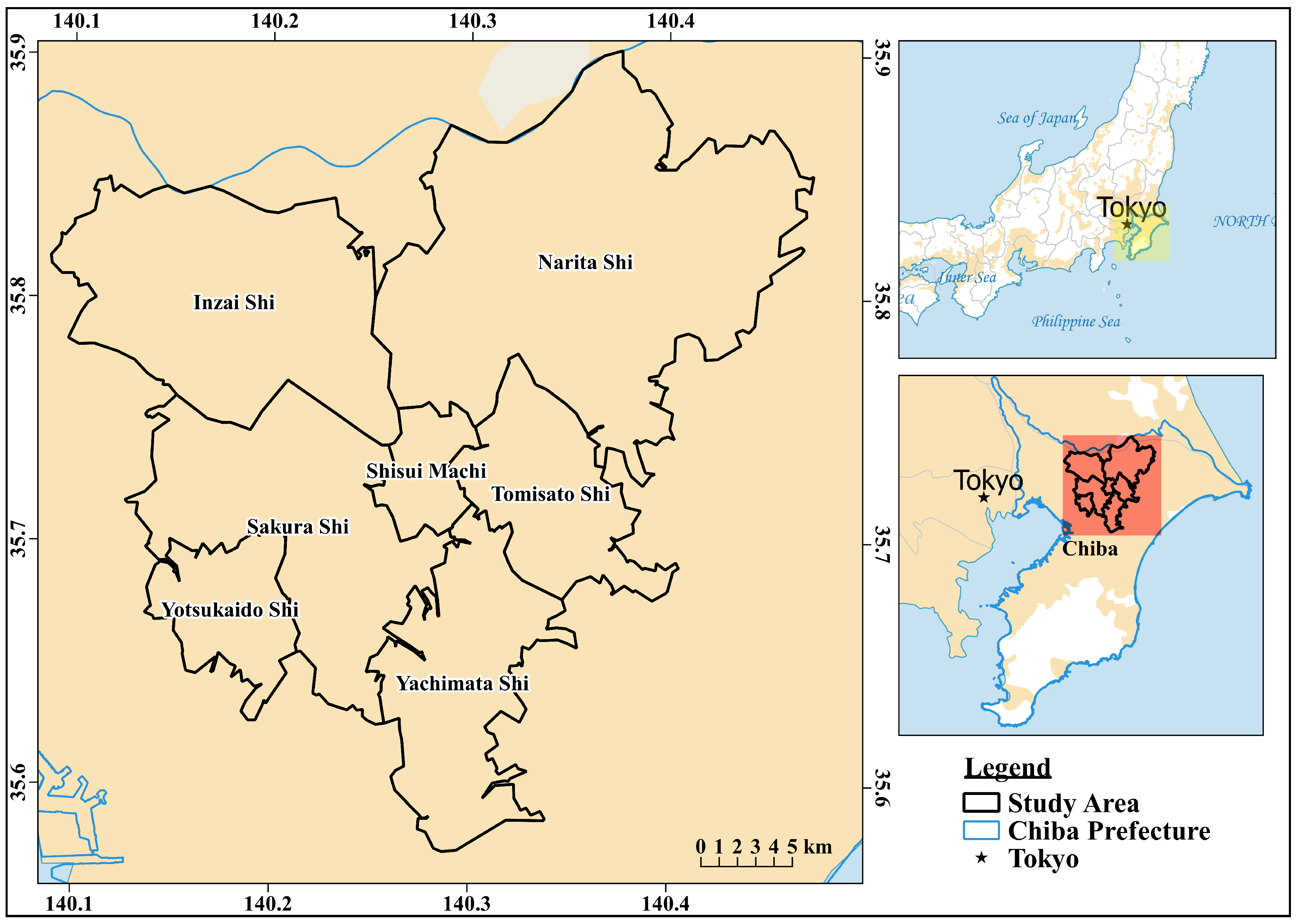
The study area, shown in Figure 1, is made up of seven municipalities within the Chiba prefecture, which is in the South-eastern part of Japan and is adjacent to the Tokyo Metropolis to the east. The seven municipalities are Yotsukaido-shi, Inzai-shi, Yachimata-shi, Narita-shi, Sakura-shi, Tomisato-shi, and Shisui-machi, with a total area of 623.15 km2 and a population of 668,603.
The Chiba prefecture is a valuable source of agricultural food crops and was ranked sixth in agricultural production in Japan, with vegetable production worth more than half a billion yen in 2015 [35]. It has a varied landscape, comprised of urban or built-up areas, forests (evergreen and deciduous), grasslands (land covered with grass or shrubs), paddy fields, croplands (also described as upland cropland), and water bodies. Grasslands in the area consist of two types: Natural and managed. On the one hand, natural grasslands contain untended grass and shrubs, and include abandoned croplands and paddy fields. On the other hand, there are the managed grasslands, such as golf courses, which are numerous due to proximity to Tokyo.
The Chiba prefecture has an annual average temperature of 16 °C, with annual and monthly average maximum and minimum temperatures of 31 °C and 2 °C, respectively. The annual average precipitation is 1496 mm, and it receives approximately 2113 h of sunlight yearly, making it highly favorable for agricultural production [35,36]. The main crops, in the regions selected, are rice (which is cultivated on irrigated paddy rice fields) and vegetables; including, but not limited to, carrot, daikon radish, taro, cabbage, and spinach.
2.2. Data Acquisition and Pre-Processing
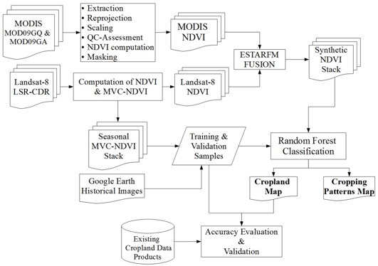
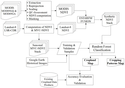
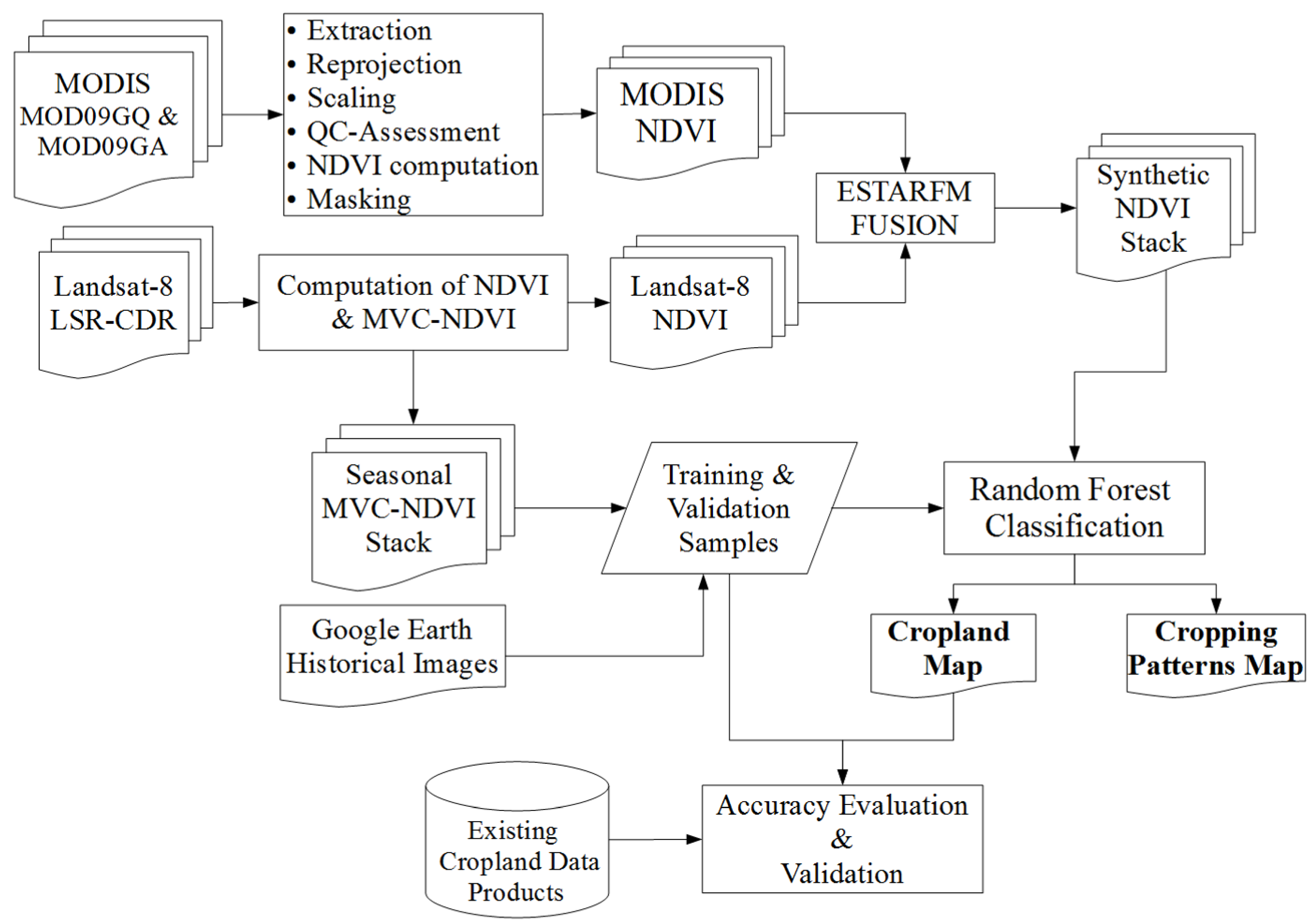
The overall flow of processing and analysis activities in this study is as depicted in Figure 2. Two satellite earth observation datasets, Landsat 8 and Moderate Resolution Imaging Spectroradiometer (MODIS) data, were acquired from the United States Geological Survey’s (USGS) EarthExplorer site [37]. Landsat 8 has a spatial resolution of 30 m and a temporal resolution of 16 days, while the MODIS data used in this study were daily 250 m images. In an initial application needs assessment, the suitability of the independent use of Landsat with respect to the study’s objectives and knowledge of the prevailing conditions on the ground was evaluated. Table 1 shows all of the images for the year 2015 for the Landsat tile, WRS Path/Row 107/035 covering the study area, and their corresponding land cloud cover. Twelve of the images had more than 30% land cloud cover and were excluded from any further evaluation.
Moreover, the period between April and September (that is, spring to fall) is critical, as crops in the field are in the vegetative phase and are thus useful for remote sensing detection. In June, July, and September, four images had 100% cloud cover—thus ruling out single sensor reconstruction [26,27]. Also, approximately 75% of the cultivated land in the study area is less than 5 Ha, as shown in Figure 3, including paddy rice fields and land under permanent crops. The Landsat 8 30-m resolution is suitable for the mapping of paddy rice fields since they are spatially contiguous, have relatively uniform cultivation and management practices, and the phenology of rice is well understood [38,39].
However, the upland croplands tend to be small, fragmented, dispersed, and have diverse cropping patterns and crop varieties, due to varied management practices. Single-date Landsat image classification would therefore not adequately capture these food production units since, at any one time, not all fields have crops and bare or fallow parcels would be classified as bare land or grassland. Thus, time-series classification was more suitable [15,23]. Further evaluation of the Landsat images for cloud cover, focussing on the study area, was carried out, and eight images were finally selected, resulting in an irregular time series.
Two daily MODIS surface reflectance products (MOD09GA and MOD09GQ) were acquired, for horizontal tile 29 and vertical tile 5 (h29v05), for the period spanning 1 January 2015 to 31 December 2015. The two surface reflectance bands contained in the MOD09GQ scientific dataset (SDS), red (620–670 nm) and near-infrared (NIR) (841–876 nm), and the state 1 km SDS in MOD09GA SDS, were extracted. MODIS data are delivered in the sinusoidal projection, and were therefore reprojected to the Universal Transverse Mercator Projection (UTM) zone 54N. The reflectance bands and state 1 km SDS were then subset to the Chiba prefecture bounds. A scale factor of 0.0001 was applied to the red and NIR bands, prior to computation of NDVI. The state 1 km SDS was used to retrieve cloud-specific information during quality assessment, because this parameter has not been populated in the reflectance band quality SDS included in the MOD09GQ product since MODIS version 3, as detailed in [40,41]. The Quality Control (QC) masks from the state 1 km SDS were resampled to 250 m using bilinear interpolation, and applied to the NDVI images through masking. The resulting daily NDVI images at 250 m resolution had gaps due to masking, and gap-filling was carried out via linear interpolation in the temporal dimension [42].
2.3. Spatio-Temporal Image Fusion
Landsat 8 irregular time-series data and daily MODIS images were fused to generate a regular time series. MODIS data supports Landsat via fusion to inform phenological traits and maintain temporal continuity in the observed phenomena [23,25]. Fusion methods are categorized by the mathematical relationships between the reference and observation data into four groups, including weighted function based, unmixing based, dictionary-pair learning based, and data-assimilation based algorithms [29,43]. The weighted function based methods include the Spatial and Temporal Adaptive Reflectance Fusion Model (STARFM) and the Enhanced STARFM (ESTARFM), which assume that no land cover type changes occur between the reference and prediction dates [43,44]. While this assumption limits the performance of weight function based algorithms in heterogeneous landscapes where rapid, abrupt changes occur, they are popular since they require no auxiliary data as inputs and are robust enough to predict pixels with changes in biophysical attributes [44,45,46]. In remote sensing, indices enhance spectral information and class separability and are, therefore, an essential basis for the estimation of the biophysical characteristics of land cover, such as vegetation vigor [44,46]. Fusion may be applied to the reflectance bands of images or the indices, via Blend-then-Index (BI) or Index-then-Blend (IB), respectively [43]. Research has found that IB is more computationally efficient and accurate, and its performance is influenced less by choice of algorithm [45,46]. Li et al. [46] found that the use of a MODIS 8-day composite surface reflectance product (MOD09A1 and MYD09A1) with a temporal mismatch between the Landsat and MODIS images resulted in weaker correlations between the observed and synthetic images, due to the day-to-day variation in the MODIS viewing geometry. Table 2 shows the relative distribution of the eight selected Landsat 8 images for this study, and the corresponding available dates in MODIS 8-day composite data, which shows a one-day difference. For this study, we used the daily MODIS surface reflectance products (MOD09GQ and MOD09GA), thus allowing the selection of a start date within the MODIS daily time-series that would fully match the available Landsat image time-series.
Spatio-temporal fusion via IB was implemented using the MODIS Daily 250 m NDVI and Landsat 8 intermittent NDVI images, as described in [45]. The MODIS NDVI images were first resampled to 30 m through bilinear interpolation to reduce the effects of geo-referencing error, then cropped to match the extent of the Landsat 8 NDVI images using R (v3.4.4) [33]. Fusion was implemented in ENVI IDL version 4.8 (Exelis Visual Information Solutions, Boulder, Colorado) using the open-source Enhanced Spatio-Temporal Adaptive Reflectance Fusion Model (ESTARFM) [47]. Many spatiotemporal fusion models have been developed, but ESTARFM has been found to be effective in generating synthetic high-resolution images for heterogeneous regions [44,45,46,47].
ESTARFM requires at least two pairs of temporally coincident fine-resolution (moderate to high spatial resolution–low temporal resolution) and coarse resolution (low spatial resolution–high temporal resolution) images as inputs. Using a specified moving window size within the image, and thereby having a central pixel, similarity of pixels with reference to the central pixel is evaluated and weights computed. Working on the assumption that, for a heterogeneous landscape, the changes in reflectance within a mixed pixel are representative of the weighted sum of changes for each land cover type, and that these changes do not occur significantly over a short period of time, the relationship then can be inferred from the pixel value of the fine resolution pixels [45]. Additionally, given that predictions for fine-resolution pixels are likely to be more accurate from a pure coarse-resolution pixel, larger weights are assigned to these pixels, and so conversion coefficients are thus computed and used to predict the fine-resolution reflectance or index value per pixel. As the objective of this study was to classify land cover annually and, specifically, to discriminate cropland from non-cropland, the prediction of land cover changes was not necessary and the ESTARFM algorithm has been found to predict phenology changes satisfactorily [43,44,45,46,47]. The fine-resolution reference images, used in the fusion process, were the most cloud-free Landsat 8 NDVI images for 2015, acquired in late winter (10th January), early spring (16th April), and mid-fall (9th and 25th October). For computational efficiency, an 8-day interval was chosen.
2.4. Training and Validation Data Collection
Two main land cover and cropland datasets were evaluated as potential sources of training and validation data. The Japan Aerospace Exploration Agency’s (JAXA’s) High Resolution Land Use and Land Cover map of Japan (HRLULC Ver.18.03) is a 30 m land cover map of Japan, generated using multi-temporal, multi-source data. The data includes Landsat 8 OLI collection 1 images, 10 m geographical and topographic data from the Geographical Survey Institute (GSI) of Japan, Advanced Land Observing Satellite (ALOS-2)/ Phased Array type L-band Synthetic Aperture Rader(PALSAR) 25 m 2015 mosaic dataset, and ALOS Panchromatic Remote-sensing Instrument for Stereo Mapping (PRISM) Digital Surface Model (DSM). A Bayesian estimation classifier, followed by post-classification editing, was used for the latest version. The JAXA High Resolution land use/land cover maps have a regular update frequency, and were identified in Waldner et al. [48] as a freely available regional cropland-related dataset for Japan. It has ten land use/land cover classes, including water, urban, rice paddy, crop, grass, deciduous hardwood forest, deciduous softwood forest, evergreen broad-leaved forest, evergreen conifers forest, and bare land. The reported producer’s and user’s accuracy for the cropland class are 83.8% and 74.1%, respectively. However, since the data used in its production is not temporally specific and ranges from 2014 to 2016, it was decided to use this dataset for validation of the results of this study. Further details on its production are available in [49].
In addition, the recently released Global Food Security-Support Analysis Data at 30 m (GFSAD30), benchmarked for 2015, was evaluated [50]. The Southeast and Northeast Asia dataset (GFSAD30SEACE) were acquired and assessed for suitability as a source of training and validation data in this study. The cropland extent in this dataset represents all cultivated land including paddy, irrigated, and rainfed areas. As the discrimination between paddy rice fields and other croplands was an objective of this study, the GFSAD30SEACE dataset was used for validation of our result, in terms of total cropland extent.
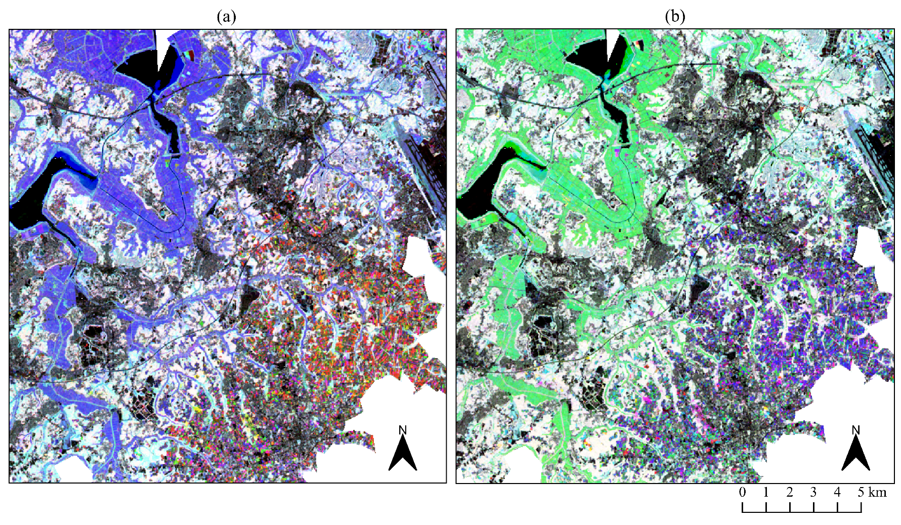
In the absence of a reference dataset that was temporally specific to the year 2015 and representative of the intended cropland class, reference data samples were generated using the Maximum Value Composite NDVI (MVC-NDVI), computed between consecutive NDVI images of the sparse Landsat image time series. In addition to minimizing the effects of cloud cover, the seasonal MVC-NDVI Red-Green-Blue (RGB) composite stacks, as shown in Figure 4, revealed inter-seasonal pixel-level NDVI changes which made it possible to determine seasonal behavior of the major land cover types and set rules for distinguishing the major land cover classes and cropping patterns. Through raster math of the MVC-NDVI layers, masks were generated for each land cover class. The raster masks were then vectorized and cleaned-up, by comparison with the Google Earth (GE) image available for 9th October 2015. A dense point cloud was then generated for each land cover class by joining the vector land cover masks with a 30 m point vector grid of the study area. The training and validation points were then selected via stratified random sampling of the dense point cloud.
In this study, distinguishing peanuts from other crops growing in the study area was tested. Peanuts, grown for their commercial value, are a popular crop in this region. Approximately 75% of Japan’s domestic supply of peanuts comes from the Chiba prefecture [51,52,53]. From moderate resolution satellite images, it is impossible to distinguish, with certainty, one crop (e.g., peanuts) from another (e.g., carrots) during the growing season. As such, to know which crop was growing at a certain location at a given time, field photos or farm surveys are necessary during the growing season in every year, since farmers regularly change crops cultivated, especially in the case of horticultural food crops. Constant and regular acquisition of crop type information is time-consuming and costly. Thus, creative means of inferring and deciphering such information from existing data are necessary. In this study, the post-harvest practice of jiboshi by peanut farmers in Japan makes it possible to know where peanuts had been growing, within at least a month from harvesting.
After harvest, peanut pods have approximately 50% moisture which renders them prone to contamination with mycotoxins, which are a major food safety concern and may lead to considerable economic losses [54,55]. Peanut farmers in the Chiba prefecture will, after harvest, leave the peanut plants and pods in inverted windrows, which allows air to circulate around the pod and for the moisture content to diminish significantly, for about a week [55]. Thereafter, the peanut plants and pods are piled into solitary heaps, as shown in Figure 5a, in a process referred to as jiboshi (drying on the ground) for about a month. These piles or heaps are referred to as bocchi, and are visible from GE images (as shown in Figure 5b), thus allowing one to infer that peanuts had been growing on that field within at least a month of acquisition of the image. Training and validation samples were collected within the study area, for locations which were visible in the GE image of 9th and 29th October 2015.
2.5. Time Series Classification
The Random Forest (RF) classification algorithm was used in this study. RF is a robust ensemble machine learning classifier, which has been used in numerous agricultural mapping application studies [56,57,58,59,60,61]. RF has been found to be stable and efficient, with better performance in classification of croplands with high intra-class variability than other classifiers, such as conventional decision trees and time-weighted dynamic time warping (TWDTW) [15,61]. In this study, RF was implemented using the RStoolbox (ver.0.2.3) package in R, by use of the ’superClass’ function [62]. The function takes, as input, the raster image and reference data—either as spatial points or a spatial polygon data frame, containing position and class attribute information. A separate validation dataset can also be provided but, if not, the training dataset is split based on a partition proportion ranging from zero to one, provided by the user. The model tuning parameters are the number of samples per land cover class, the number of levels for each tuning parameter, and the number of cross-validation resamples, for robust prediction performance [56]. To ensure non-overlap between training and validation data, a minimum distance, in terms of pixels, can be provided [62]. Several combinations of the tuning parameters, informed by the RStoolbox package literature, were tested with a 70% training data and 30% validation data split. The configuration with the best sensitivity in the cropland class was chosen.
2.6. Accuracy Assessment
The classification results were evaluated using error matrix accuracy assessment metrics, which include producer’s, user’s, and overall accuracy, as well as the kappa coefficient, as defined in Equation (1). The mathematical notation of the kappa coefficient, with respect to the error matrix, is shown in Equation (2) [63,64].
where is the kappa coefficient, N is the total number of observations, r is the number of rows in the error matrix, xii is the number of observations in row i and column i, and xi+ and x+i are the marginal totals of row i and column i, respectively [64]. The kappa coefficient provides a measure of how much better the classification performed, compared to the probability of randomly assigning pixels to the correct class.
3. Results
3.1. Fusion Results
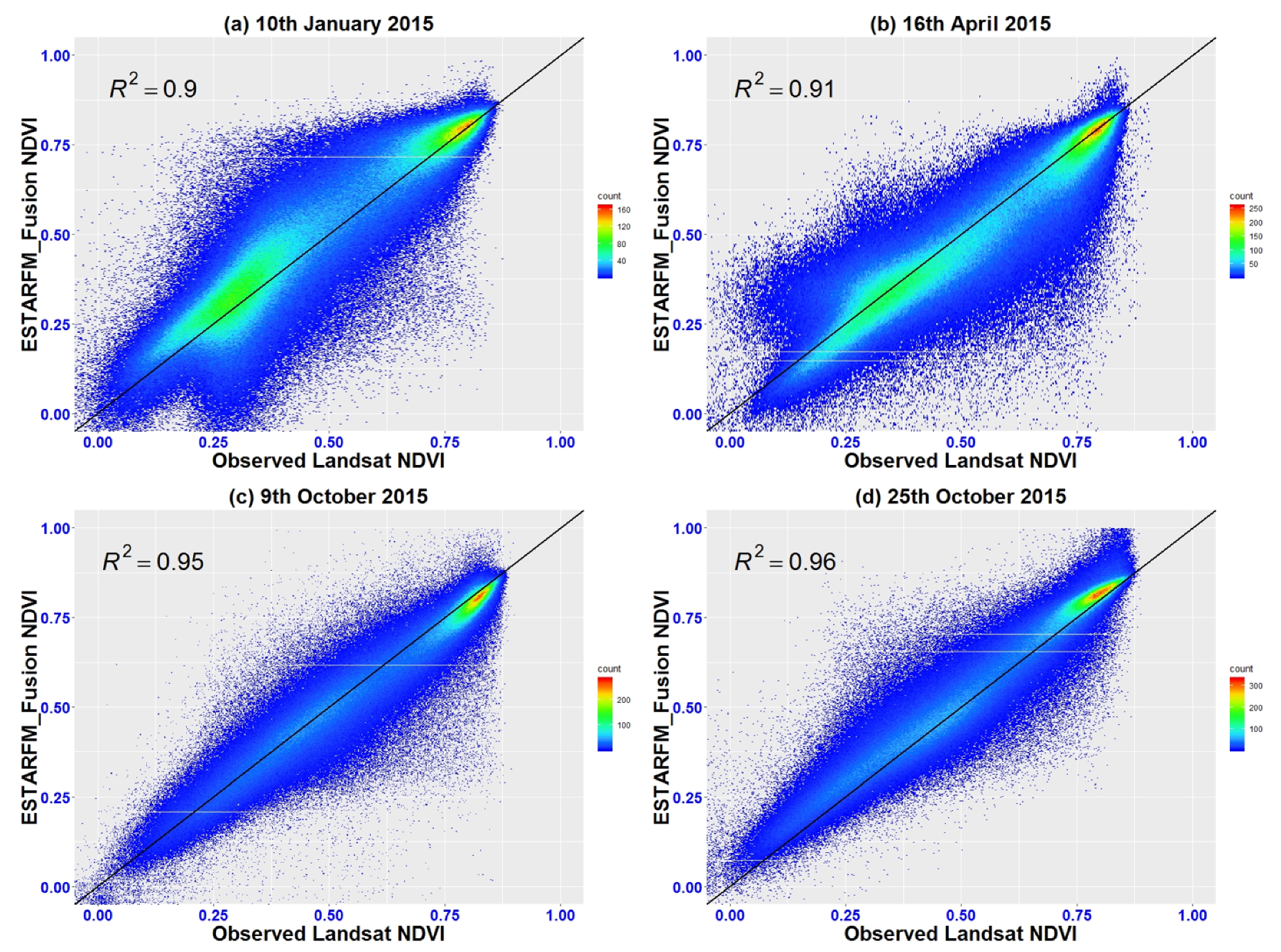
Performance of the fusion process in generating synthetic NDVI images was evaluated quantitatively by comparing the synthetic NDVI images to the reference observed Landsat NDVI images. Overall, there was a strong agreement between the synthetic images and the observed Landsat images, with R2 > 0.9 for all dates, as depicted in Figure 6. A higher association was found in the mid-fall images (9th and 25th October) (Figure 6c,d), than in the late winter (10th January) (Figure 6a) and early spring (16th April) (Figure 6b) images. Phenological changes in the landscape can also be inferred from the point density in the scatterplots, shown by color—with blue being low density and red showing high density. In the late winter and early spring images (when vegetation vigor is low), there are two data clusters. The first, albeit lower density, lies in the mid NDVI ranges (0.125 to 0.5), and the second within the higher NDVI ranges (0.6 to 0.8). However, in the mid-fall images (when vegetation vigor is high), the scatterplot tapers with high density in the higher NDVI ranges. This may be attributed to the intra-annual changes in vegetation density, and is demonstrative of more pure vegetation pixels in the fall than in late winter and early spring. These observations may not hold for other years of study for the same region, or other regions with different land cover and climate, and require further investigation.
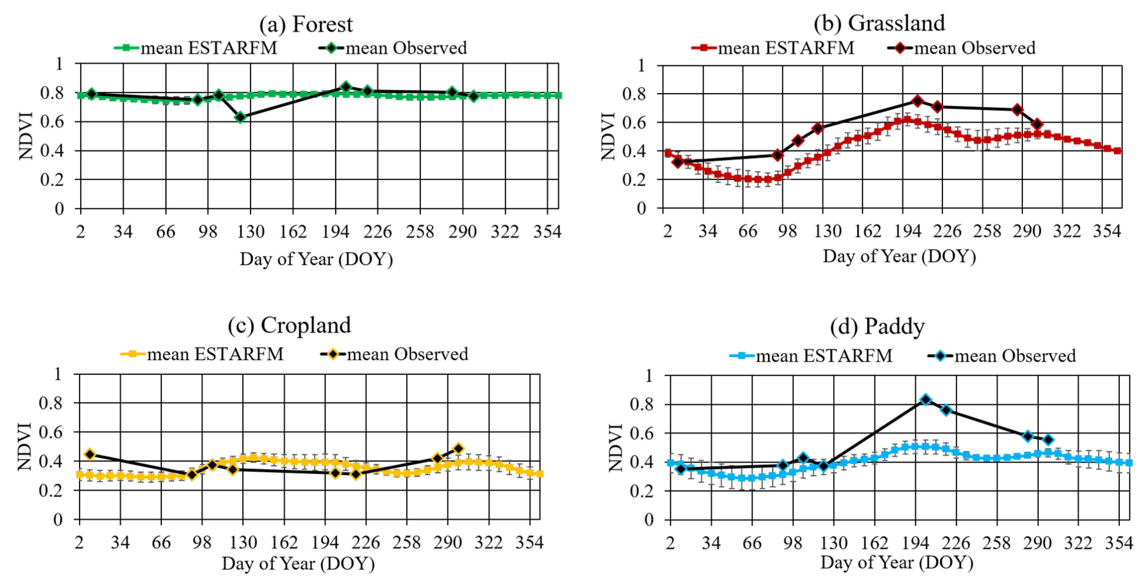
Figure 7 shows the qualitative assessment of the fusion results, in terms of the temporal evolution of NDVI in the smoothed fusion series and the original Landsat 8 series for the main vegetation cover types in the study area. The shape or configuration of the temporal profiles of the synthetic NDVI time series are analogous to those of the observed NDVI, for all of the main vegetation cover classes. The standard error in the synthetic NDVI time-series are also reflective of intra-class behavior. For forest or dense vegetation, there is minimal variation throughout the year also detected in the observed MVC-NDVI, as shown in Figure 4.
Internal variability is exhibited in the other vegetation types, and varies with season. In the case of the grassland temporal evolution of NDVI, sample points were taken from both the artificial and natural grasslands, and therefore exhibit high intra-class variability. However, towards the end of the year (as winter commences), vegetation vigor decreases and the intra-class variability diminishes, as seen from the error bars in that profile. The observed images do not cover this later part of the temporal behavior of the grassland land cover, as the series ends in early fall, and demonstrates the predictive capabilities of the ESTARFM fusion model. Based on the temporal information inferred from the available coarse resolution images, the changes in the biophysical characteristics of land cover features can be elicited, even in the absence of complete annual coverage of the fine resolution images.
The temporal profiles of the cropland and paddy classes also reveal characteristics inherent to these land cover classes. Intra-class variability in the cropland class exhibits a double cropping pattern, where fluctuations are detected during the growing seasons and abate (albeit minimally when the curve is in decline and recovery). Contrastingly, for the paddy class, fluctuations are detected most when it is expected that paddy rice is not on-field. That is, January to April and October to December, or late winter to spring and late fall into the winter. This behavior is akin to that observed within the grassland class, and is indicative of post-harvest vegetation whose vigor is not subject to management practices by the farmer. However, as in the case of grassland land cover, the concluding part of the year and the information elicited arises from the synthetic dataset, and would not have been available within the available Landsat imagery. Overall, both the quantitative and qualitative assessments of the fusion result, in comparison to the observed Landsat dataset, vis-à-vis conventional land cover temporal changes, establish the value of fusion in providing information about land cover prior to classification. Figure 8 depicts the temporal evolution of NDVI in the synthetic time-series stack for representative sample points in the major land cover types of the study area. From this graph, the significance of the synthetic time-series dataset is substantiated further, since we see that for grassland, paddy, and cropland, the spring-summer seasons provide the best distinction points with continuity. The observed Landsat image time-series was sparse, due to inundation with cloud cover during this crucial period, hence making information unavailable; especially in the cropland class.
3.2. Classification Results
3.2.1. Cropland Extent
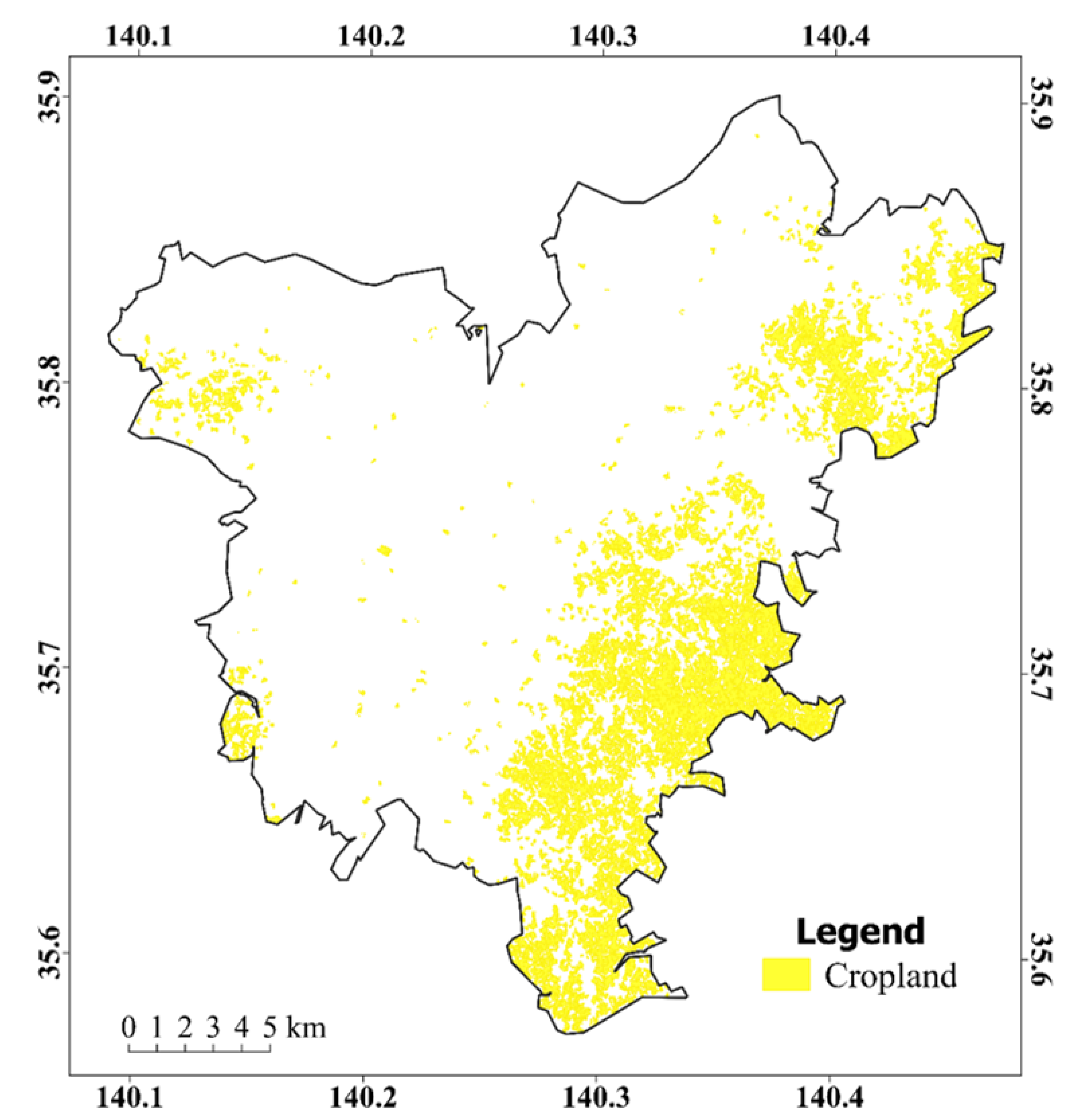
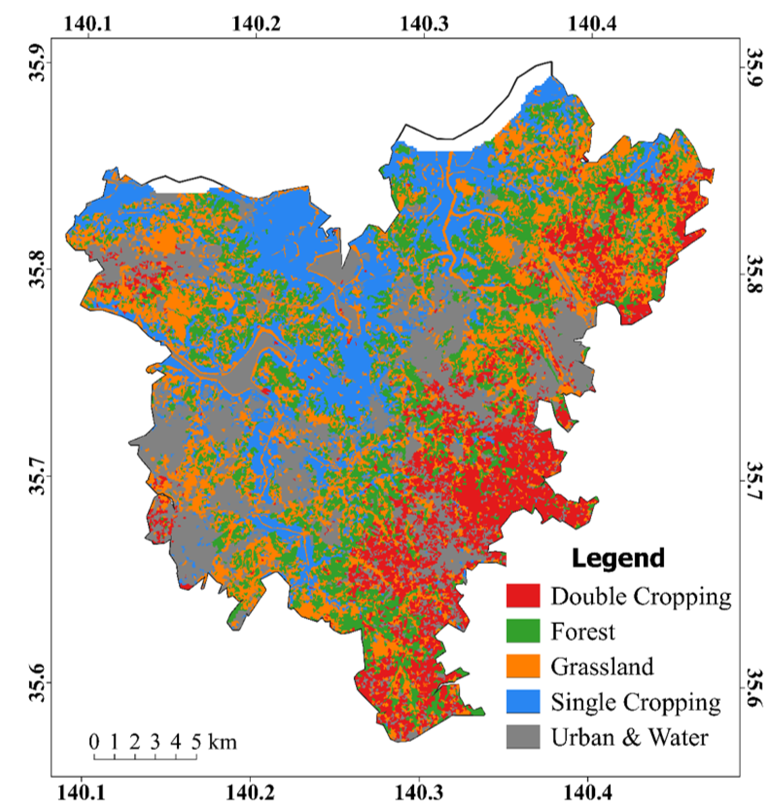
The cropland extent in the context of this study is all land used for crop cultivation, excluding paddy fields. An initial land use/land cover classification was carried out for the main land use/cover types in the region, as shown in Figure 9. An overall accuracy of 91.7% was achieved, with a stratified random sample of over 1000 points per class. The dominant land use/cover classes of forest, grassland, paddy, and urban and water had the highest producer’s (PA) and user’s accuracies (UA), both more than 90%. The cropland area estimation had the lowest PA and UA, of 79.8% and 86.4%, respectively, but was deemed to be acceptable, given the heterogeneity of the landscape. The estimated area of croplands, excluding paddy fields, for the study area in 2015 was 85.5 Km2, as is depicted in Figure 10. Table 3 shows the classification’s error matrix. Vegetation along urban features and banks of water bodies were also misclassified as cropland and paddy. Within the paddy field class, the timing of post-harvest vegetation in the fall within some paddy fields manifested as two peaks, similar to croplands with double cropping, leading to misclassification as croplands.
3.2.2. Cropping Regimes
Two main cropping patterns or regimes were estimated, as shown in Figure 11: Single cropping, where a pixel had a singular peak within the year, in a season or within two consecutive seasons; and double cropping, for pixels with two peaks in non-consecutive seasons—that is, winter-summer, winter-fall, and spring-fall. The cropping regimes estimation confusion matrix is as shown in Table 4. Most of the croplands were found to be under double cropping intensity, while paddy rice was under single cropping. This is expected, since the upland cropland is used mainly for the production of horticultural food crops that have short durations of growth. Table 5 shows the best periods of market availability for some of the Chiba prefecture’s representative crops. This table can be taken to represent an inverse crop calendar, where periods of non-availability represent the growing periods. Therefore, apart from taro and peanuts, which have high market availability for only one period within a year, the rest of the crops can be said to be planted twice by one farmer or continuously by various farmers, within the year. Taro has a long growth period between transplanting and maturation, approximately six to eight months. The table also does not take into account market availability as a result of imports from other regions or countries. Consequently, it is expected that most upland croplands will exhibit double cropping, as our result indicates. Most paddy rice fields had a single cropping pattern, with the exception of a few. This can be attributed to the fact that paddy rice fields are highly sensitive to changes in soil composition, and therefore farmers prefer to leave the land fallow post-harvest in order to maintain the soil nutrient balance necessary for paddy rice. In addition, paddy rice cultivation is a highly specialized skill in Japan and is resource- and labor-intensive. Therefore, apart from the cultivation of other crops for subsistence consumption, which is normally carried out on other parcels of land, paddy rice farmers tend to focus only on paddy rice.
3.2.3. Peanuts and Other Crops
A total of 378 sample points representing peanuts were collected, as described in Section 2.4. Non-cropland land cover classes including forest, grassland, paddy, and urban and water were masked out from the fusion time-series, using the cropland mask produced in this study. A stratified random sampling of the peanut samples and other croplands not designated as peanuts was carried out to yield 200 points per class, and a binary classification was implemented. The overall accuracy was 67.1%, and the PA and UA for the peanut class were 63.2% and 71.2%, respectively. Given the limited amount of reference data and the fact that peanuts are cultivated at the same time as other crops, as seen in Table 5, we found this classification accuracy to be sufficient. The phenological similarity between peanuts and other crops, as well as high intra-class variability within the cropland class, requires that a large number of training datasets is used to train the RF classifier [57]. Further research on the determination of the distinct spectral-temporal characteristics of peanuts and other crops cultivated in the region, with more training data and predictors, could improve the classification accuracy.
4. Discussion
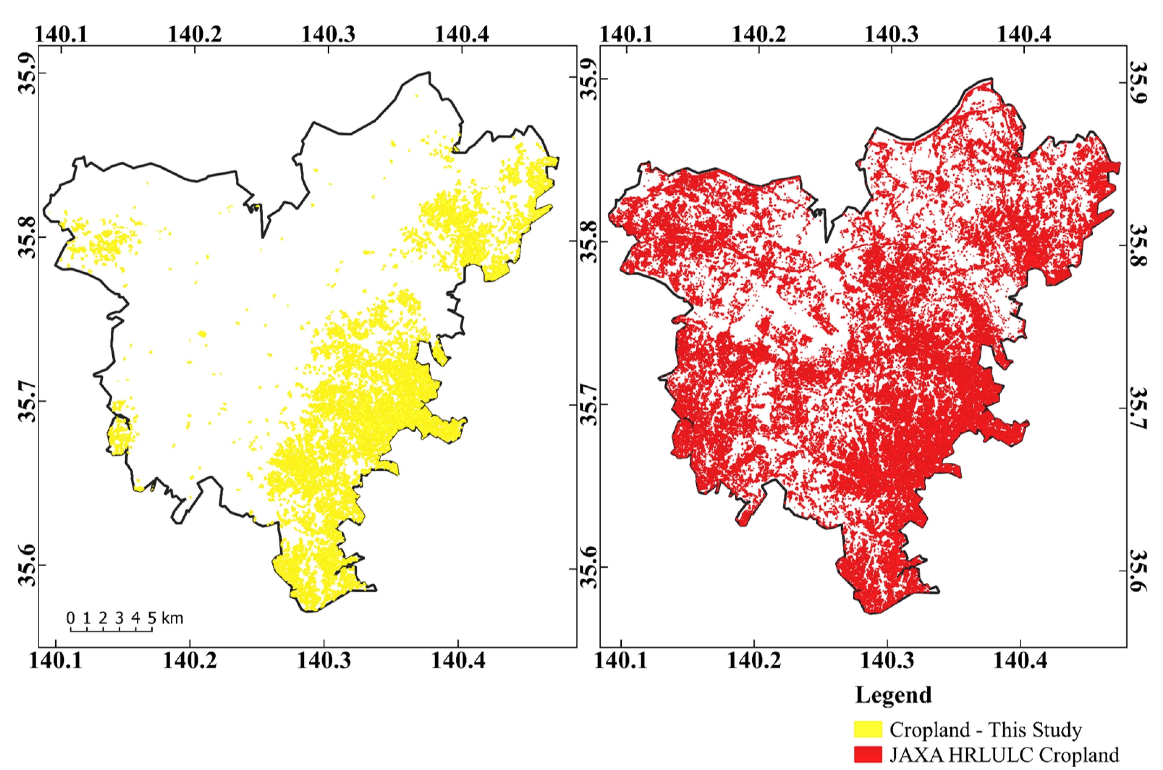
In this study, the application of a high temporal density image time-series to intra-annual cropland extent and cropping regime estimation was evaluated. Validation of the cropland extent or distribution was carried out by comparing this study’s result with two existing cropland maps; that is, the regional JAXA HRLULC and the global GFSAD30SEACE datasets. The upland cropland extent, according to the JAXA HRLULC (version 18.03) map, was approximately 367.9 Km2, while, in the GFSAD30SEACE data set (which includes paddy fields), it was 129.4 Km2. The cropland extent in this study was 85.5 Km2. Sharma et al. [65] produced a land use/land cover map of Japan for 2013 to 2015, the JpLC-30 map, and compared their result to the JAXA HRLULC map (version 14.02). Disparities between the JpLC-30m map and the JAXA HRLULC map (version 14.02) were detected, including: Croplands in forests, water-bodies in forests, water in croplands, and herbaceous land cover in croplands. Based on this comparison, the classification of croplands in the JAXA HRLULC map (version 14.02) was severely affected. The improvement over the earlier version (16.03) in cropland classification accuracy is significant. In version 16.03, the reported producer’s and user’s accuracy for the cropland class were 63.9% and 45.2%, respectively, while, in version 18.03, the producer’s and user’s accuracy for the cropland class were 83.8% and 74.1%, respectively. Figure 12 depicts the cropland extent, as per this study, excluding paddy fields, and the JAXA HRLULC (version 18.03) cropland. The cropland extent within the JAXA HRLULC (version 18.03) map far exceeds the extent in this study. Further inspection of the land use/land cover map shows misclassification of urban land cover as cropland in the JAXA map, as shown in Figure 13. This phenomenon, which has also been observed in other regional land use/land cover maps, such as the GlobeLand30 map, may be attributed to spatial heterogeneity, but further investigations are necessary [46].
Figure 14 shows our cropland and paddy extent, and the GFSAD30SEACE cropland extent. The GFSAD30 product does not make a distinction between types of croplands—that is, upland cropland and paddy rice—and, while it adequately captures the paddy fields and compares favorably with our result, it underestimates the upland cropland. This may be attributed to the heterogeneous nature of the upland croplands, which leads to misclassification of upland cropland as non-cropland in the GFSAD30 framework. Our result overestimated paddy fields, with commission errors of 2.3% and 4.15% as cropland and grassland, respectively. However, this was almost balanced out by misclassification of some paddy fields as croplands, and can be attributed to the fact that only NDVI was used as a classification metric. Using other metrics for the same one-year data-set, such as the NDWI index or shape and texture features, may solve this [66].
Statistical survey data at local and national scales can be useful in assessing the results of remote sensing classification and estimates. While it can be time consuming and expensive, it allows for various government agencies and stakeholders to engage directly with farmers. However, there is no standard approach to collection and dissemination of such data and, for regional and global upscaling, statistical data can prove to be problematic due to (among other issues) language barriers. Understanding what variables are measured and how they are measured is key to consideration of statistical data for reference.
Japan carries out an agricultural census every five years via questionnaires, and the last census was released on 1 February 2015. It is, therefore, not representative of the agricultural production situation in the year 2015 but, rather, represents the preceding five years. Farmers respond to questionnaires by regions referred to as ‘agricultural villages’, and respond to (among other questions) how much land is under cultivation, whether the production is for commercial or subsistence purposes, and what they grow. However, the boundaries of the agricultural villages do not match the current national administrative boundaries. This, therefore, makes merging and comparison of this data with data obtained based on administrative boundaries difficult. The total reported area of cropland in the statistical data was 129.5 Km2. This figure is close to our estimated area of paddy rice fields (123.21 Km2), and also matches the GFSAD30 cropland area. Spatial distribution of crops and cropping regimes could not be inferred, due to the incongruence between the boundaries used in this study with those of the statistical data. The results of this study, therefore, provide a base-map compatible with national administrative boundaries, for future analysis and monitoring of agriculture in the region.
The fusion results confirmed that implementing Index-then-Blend with MODIS dates matching the Landsat dates generates synthetic images with a strong agreement with the observed images. However, the fusion process takes a long time and, for this reason, we applied fusion to a subset of the Landsat scene covering the Chiba prefecture, rather than the entire scene. This led to the loss of data in the northern part of our study area, which also coincides with the boundary of Chiba prefecture. It would, therefore, be better to apply fusion to entire Landsat scenes or a mosaic of scenes, then subset to the intended study area.
This study demonstrates that using the simple, yet robust, NDVI with high temporal frequency, dynamic heterogeneous landscapes can be adequately mapped and monitored using data available within a year. From a policy development perspective, this aspect of our methodology is desirable, as it allows for changes taking place within the landscape to be catalogued using the most recent data and disseminated with reasonable frequency and accuracy.
5. Conclusions
Intra-annual cropland area estimation and distinction from other land cover types in heterogeneous landscapes can be challenging, due to inadequate information. In this study, we demonstrated how, using the intermittent moderate resolution Landsat and daily MODIS surface reflectance imagery, information that can be used to distinguish croplands from other land cover types can be retrieved. Fusion of the MODIS NDVI and Landsat NDVI images yielded synthetic Landsat imagery with R2 > 0.9, indicating strong agreement with the observed NDVI. The regular moderate resolution image time-series, with an 8-day interval, proved to be adequate for the task of estimating cropland area and cropping patterns in a complex heterogeneous urban landscape. In addition, using knowledge of post-harvest practices of peanut farmers in the region, we were able to distinguish peanuts from other crops with reasonable accuracy. The Random Forest classifier requires a large amount of training data, which was acquired based on the seasonal MVC-NDVI. However, this was made possible by the availability of images in each season which met the cloud-cover threshold, and may not be the case when carrying out analysis in other years or regions that are heavily inundated with cloud cover. In this regard, efforts to establish spectral-temporal libraries for various land cover types in disparate geographical locations would go a long way in enhancing local- and national-scale annual cropland mapping. This study also demonstrates the importance of local-scale cropland mapping towards validating regional- and global-scale cropland datasets. Future research work will involve evaluation of the applicability of the methodology to larger regions, and in different geographical locations which have different land cover and climate characteristics.
Author Contributions
E.N. formulated the research design and methodology, processed and analyzed the data and wrote the final manuscript. A.M. assisted in refining the methodology and revising the manuscript. Y.S. assisted in revising the manuscript. A.K., Y.W., and J.G.P. revised the manuscript and supervised. All authors contributed and approved the final manuscript before submission.
Funding
This research was funded by the Japan International Cooperation Agency (JICA), grant number D1511645.
Acknowledgments
The authors would like to thank the reviewers and the editors for the invaluable and constructive comments and suggestions. Eunice Nduati is grateful to the Japan International Cooperation Agency (JICA) for the financial support that made this work possible.
Conflicts of Interest
The authors declare no conflict of interest. The funders had no role in the design of the study; in the collection, analyses, or interpretation of data; in the writing of the manuscript, and in the decision to publish the results.
References
- Brown, M.E.; Funk, C.C. Food security under climate change. Nat. Clim. Chang. 2008, 6, 10–13. [Google Scholar] [CrossRef] [PubMed]
- Porter, J.R.; Dyball, R.; Dumaresq, D.; Deutsch, L.; Matsuda, H. Feeding capitals: Urban food security and self-provisioning in Canberra, Copenhagen and Tokyo. Glob. Food Secur. 2014, 3, 1–7. [Google Scholar] [CrossRef]
- Eigenbrod, C.; Gruda, N. Urban vegetable for food security in cities. A review. Agron. Sustain. Dev. 2015, 35, 483–498. [Google Scholar] [CrossRef]
- Opitz, I.; Berges, R.; Piorr, A.; Krikser, T. Contributing to food security in urban areas: Differences between urban agriculture and peri-urban agriculture in the Global North. Agric. Hum. Values 2016, 33, 341–358. [Google Scholar] [CrossRef]
- Besthorn, F.H. Vertical farming: Social work and sustainable urban agriculture in an age of global food crises. Aust. Soc. Work 2013, 66, 187–203. [Google Scholar] [CrossRef]
- Lang, T.; Barling, D. Food security and food sustainability: Reformulating the debate. Geogr. J. 2012, 178, 313–326. [Google Scholar] [CrossRef]
- Thebo, A.L.; Drechsel, P.; Lambin, E.F. Global assessment of urban and peri-urban agriculture: Irrigated and rainfed croplands. Environ. Res. Lett. 2014, 9, 114002. [Google Scholar] [CrossRef]
- Martellozzo, F.; Landry, J.S.; Plouffe, D.; Seufert, V.; Rowhani, P.; Ramankutty, N. Urban agriculture: A global analysis of the space constraint to meet urban vegetable demand. Environ. Res. Lett. 2014, 9, 064025. [Google Scholar] [CrossRef]
- d’Amour, C.B.; Reitsma, F.; Baiocchi, G.; Barthel, S.; Güneralp, B.; Erb, K.; Haberl, H.; Creutzig, F.; Seto, K.C. Future urban land expansion and implications for global croplands. Proc. Natl. Acad. Sci. USA 2017, 114, 8939–8944. [Google Scholar] [CrossRef]
- Waldner, F.; Canto, G.S.; Defourny, P. Automated annual cropland mapping using knowledge-based temporal features. ISPRS J. Photogramm. Remote Sens. 2015, 110, 1–13. [Google Scholar] [CrossRef]
- Thenkabail, P.S. Global Food Security Support Analysis Data at Nominal 1 km (GFSAD1km) Derived from Remote Sensing in Support of Food Security in the Twenty-First Century: Current Achievements and Future Possibilities. In Remote Sensing Handbook-Three Volume Set; CRC Press: Boca Raton, FL, USA, 2019; pp. 865–894. [Google Scholar]
- Teluguntla, P.; Thenkabail, P.S.; Xiong, J.; Gumma, M.K.; Congalton, R.G.; Oliphant, A.; Poehnelt, J.; Yadav, K.; Rao, M.; Massey, R. Spectral matching techniques (SMTs) and automated cropland classification algorithms (ACCAs) for mapping croplands of Australia using MODIS 250-m time-series (2000–2015) data. Int. J. Digit. Earth 2017, 10, 944–977. [Google Scholar] [CrossRef] [Green Version]
- Teluguntla, P.; Thenkabail, P.; Oliphant, A.; Xiong, J.; Gumma, M.K.; Congalton, R.G.; Yadav, K.; Huete, A. A 30-m Landsat-derived cropland extent product of Australia and China using random forest machine learning algorithm on Google Earth Engine cloud computing platform. ISPRS J. Photogramm. Remote Sens. 2018, 144, 325–340. [Google Scholar] [CrossRef]
- Matton, N.; Canto, G.S.; Waldner, F.; Valero, S.; Morin, D.; Inglada, J.; Arias, M.; Bontemps, S.; Koetz, B.; Defourny, P. An automated method for annual cropland mapping along the season for various globally-distributed agrosystems using high spatial and temporal resolution time series. Remote Sens. 2015, 7, 13208–13232. [Google Scholar] [CrossRef]
- Belgiu, M.; Csillik, O. Sentinel-2 cropland mapping using pixel-based and object-based time-weighted dynamic time warping analysis. Remote Sens. Environ. 2018, 204, 509–523. [Google Scholar] [CrossRef]
- Jakubauskas, M.E.; Legates, D.R.; Kastens, J.H. Crop identification using harmonic analysis of time-series AVHRR NDVI data. Comput. Electron. Agric. 2002, 37, 127–139. [Google Scholar] [CrossRef]
- Mingwei, Z.; Zhou, Q.; Chen, Z.; Liu, J.; Zhou, Y.; Cai, C. Crop discrimination in Northern China with double cropping systems using Fourier analysis of time-series MODIS data. Int. J. Appl. Earth Obs. Geoinf. 2008, 10, 476–485. [Google Scholar] [CrossRef]
- McNairn, H.; Champagne, C.; Shang, J.; Holmstrom, D.; Reichert, G. Integration of optical and Synthetic Aperture Radar (SAR) imagery for delivering operational annual crop inventories. ISPRS J. Photogramm. Remote Sens. 2009, 64, 434–449. [Google Scholar] [CrossRef]
- Siachalou, S.; Mallinis, G.; Tsakiri-Strati, M. A hidden Markov models approach for crop classification: Linking crop phenology to time series of multi-sensor remote sensing data. Remote Sens. 2015, 7, 3633–3650. [Google Scholar] [CrossRef]
- Inglada, J.; Arias, M.; Tardy, B.; Hagolle, O.; Valero, S.; Morin, D.; Dedieu, G.; Sepulcre, G.; Bontemps, S.; Defourny, P.; et al. Assessment of an operational system for crop type map production using high temporal and spatial resolution satellite optical imagery. Remote Sens. 2015, 7, 12356–12379. [Google Scholar] [CrossRef]
- Immitzer, M.; Vuolo, F.; Atzberger, C. First experience with Sentinel-2 data for crop and tree species classifications in central Europe. Remote Sens. 2016, 8, 166. [Google Scholar] [CrossRef]
- Vladimir, C.; Lugonja, P.; Brkljač, B.N.; Brunet, B. Classification of small agricultural fields using combined Landsat-8 and RapidEye imagery: Case study of northern Serbia. J. Appl. Remote Sens. 2014, 8, 083512. [Google Scholar]
- Gómez, C.; White, J.C.; Wulder, M.A. Optical remotely sensed time series data for land cover classification: A review. ISPRS J. Photogramm. Remote Sens. 2016, 116, 55–72. [Google Scholar] [CrossRef] [Green Version]
- Petitjean, F.; Jordi, I.; Pierre, G. Satellite image time series analysis under time warping. IEEE Trans. Geosci. Remote Sens. 2012, 50, 3081–3095. [Google Scholar] [CrossRef]
- Petitjean, F.; Kurtz, C.; Passat, N.; Gançarski, P. Spatio-temporal reasoning for the classification of satellite image time series. Pattern Recognit. Lett. 2012, 33, 1805–1815. [Google Scholar] [CrossRef] [Green Version]
- Shen, H.; Li, X.; Cheng, Q.; Zeng, C.; Yang, G.; Li, H.; Zhang, L. Missing information reconstruction of remote sensing data: A technical review. IEEE Geosci. Remote Sens. Mag. 2015, 3, 61–85. [Google Scholar] [CrossRef]
- Cheng, Q.; Shen, H.; Zhang, L.; Peng, Z. Missing Information Reconstruction for Single Remote Sensing Images Using Structure-Preserving Global Optimization. IEEE Signal Process. Lett. 2017, 24, 1163–1167. [Google Scholar] [CrossRef]
- Julien, Y.; Sobrino, J.A. Comparison of cloud-reconstruction methods for time series of composite NDVI data. Remote Sens. Environ. 2010, 114, 618–625. [Google Scholar] [CrossRef]
- Zhao, Y.; Huang, B.; Song, H. A robust adaptive spatial and temporal image fusion model for complex land surface changes. Remote Sens. Environ. 2018, 208, 42–62. [Google Scholar] [CrossRef]
- Pohl, C.; Van Genderen, J.L. Review article multisensor image fusion in remote sensing: Concepts, methods and applications. Int. J. Remote Sens. 1998, 19, 823–854. [Google Scholar] [CrossRef]
- Solberg, A.H.S. Data fusion for remote sensing applications. Signal Image Process. Remote Sens. 2006, 249–271. [Google Scholar]
- Schmitt, M.; Zhu, X.X. Data fusion and remote sensing: An ever-growing relationship. IEEE Geosci. Remote Sens. Mag. 2016, 4, 6–23. [Google Scholar] [CrossRef]
- R Core Team. R: A Language and Environment for Statistical Computing; R Foundation for Statistical Computing: Vienna, Austria, 2013; Available online: http://www.R-project.org/ (accessed on 19 April 2018).
- QGIS Development Team. QGIS Geographic Information System. Open Source Geospatial Foundation. 2009. Available online: http://qgis.osgeo.org (accessed on 10 March 2018).
- Ministry of Agriculture, Forestry and Fisheries(MAFF), Japan. FY 2016 Summary of the Annual Report on Food, Agriculture and Rural Areas in Japan. 2016. Available online: http://www.maff.go.jp/j/wpaper/w_maff/h28/attach/pdf/index-28.pdf (accessed on 16 October 2018).
- Tivy, J. Agricultural Ecology; Routledge: Abingdon-on-Thames, UK, 2014. [Google Scholar]
- EarthExplorer. Available online: https://earthexplorer.usgs.gov/ (accessed on January 2018).
- Mosleh, M.; Hassan, Q.; Chowdhury, E. Application of remote sensors in mapping rice area and forecasting its production: A review. Sensors 2015, 15, 769–791. [Google Scholar] [CrossRef] [PubMed]
- Motohka, T.; Nasahara, K.N.; Miyata, A.; Mano, M.; Tsuchida, S. Evaluation of optical satellite remote sensing for rice paddy phenology in monsoon Asia using a continuous in situ dataset. Int. J. Remote Sens. 2009, 30, 4343–4357. [Google Scholar] [CrossRef]
- NASA LP DAAC. MODIS Land Products Quality Assurance Tutorial: Part-1. 2013. Available online: https://lpdaac. usgs. gov/sites/default/files/public/modis/docs/MODIS_LP_QA_Tutorial-2. pdf (accessed on 23 February 2018).
- Vermote, E. MOD09A1 MODIS/Terra Surface Reflectance 8-Day L3 Global 500m SIN Grid V006; NASA EOSDIS Land Processes DAAC: Sioux Falls, SD, USA, 2015; Volume 10.
- Lobell, D.B.; Asner, G.P. Cropland distributions from temporal unmixing of MODIS data. Remote Sens. Environ. 2004, 93, 412–422. [Google Scholar]
- Liao, C.; Wang, J.; Pritchard, I.; Liu, J.; Shang, J. A spatio-temporal data fusion model for generating NDVI time series in heterogeneous regions. Remote Sens. 2017, 9, 1125. [Google Scholar] [CrossRef]
- Zhu, X.; Chen, J.; Gao, F.; Chen, X.; Masek, J.G. An enhanced spatial and temporal adaptive reflectance fusion model for complex heterogeneous regions. Remote Sens. Environ. 2010, 114, 2610–2623. [Google Scholar] [CrossRef]
- Jarihani, A.A.; McVicar, T.R.; van Niel, T.G.; Emelyanova, I.V.; Callow, J.N.; Johansen, K. Blending Landsat and MODIS data to generate multispectral indices: A comparison of “Index-then-Blend” and “Blend-then-Index” approaches. Remote Sens. 2014, 6, 9213–9238. [Google Scholar] [CrossRef]
- Li, L.; Zhao, Y.; Fu, Y.; Pan, Y.; Yu, L.; Xin, Q. High resolution mapping of cropping cycles by fusion of landsat and MODIS data. Remote Sens. 2017, 9, 1232. [Google Scholar] [CrossRef]
- Remote Sensing and Spatial Analysis Lab, ESTARFM. 27 July 2018. Available online: https://xiaolinzhu.weebly.com/open-source-code.html (accessed on 10 March 2018).
- Waldner, F.; Fritz, S.; di Gregorio, A.; Defourny, P. Mapping priorities to focus cropland mapping activities: Fitness assessment of existing global, regional and national cropland maps. Remote Sens. 2015, 7, 7959–7986. [Google Scholar] [CrossRef]
- Japan High Resolution Land Use Land Cover (2014~2016) (Version 18.03). Available online: https://www.eorc.jaxa.jp/ALOS/lulc/lulc_jindex_v1803.htm (accessed on 9 February 2018).
- Oliphant, A.J.; Thenkabail, P.S.; Teluguntla, P.; Xiong, J.; Congalton, R.G.; Yadav, K.; Massey, R.; Gumma, M.K.; Smith, C. NASA Making Earth System Data Records for Use in Research Environments (MEaSUREs) Global Food Security-support Analysis Data (GFSAD) Cropland Extent 2015 Southeast Asia 30 m V001; NASA EOSDIS Land Processes DAAC, USGS Earth Resources Observation and Science (EROS); NASA EOSDIS Land Processes DAAC: Sioux Falls, SD, USA, 2017.
- Japan CROPs. Available online: https://japancrops.com/en/prefectures/chiba/ (accessed on 16 October 2018).
- Japan External Trade Organization (JETRO). Jitsukawa Foods: Chiba: A Peanut Paradise. Available online: https://www.jetro.go.jp/en/mjcompany/jitsukawafoods.html (accessed on 16 October 2018).
- Ito, K.; Aoki, S.T.; Shimuzu, A. Japan’s Peanut Market Report. Global Agricultural Information Network; USDA Foreign Agricultural Service; GAIN Report Number: JA9532; 22 December 2009. Available online: https://www.fas.usda.gov/ (accessed on 16 October 2018).
- Dickens, J.W. Peanut curing and post-harvest physiology. In Peanuts Culture and Uses; APRES Inc.: Roanoke, VA, USA, 1973. [Google Scholar]
- Allen, W.S.; and Sorenson, J.W.; Person, N.K., Jr. Guide for Harvesting, Handling and Drying Peanuts; No. 1029; Texas Agricultural Extension Service: College Station, TX, USA, 1971. [Google Scholar]
- Sonobe, R.; Tani, H.; Wang, X.; Kobayashi, N.; Shimamura, H. Random forest classification of crop type using multi-temporal TerraSAR-X dual-polarimetric data. Remote Sens. Lett. 2014, 5, 157–164. [Google Scholar] [CrossRef] [Green Version]
- Tatsumi, K.; Yamashiki, Y.; Torres, M.A.C.; Taipe, C.L.R. Crop classification of upland fields using Random forest of time-series Landsat 7 ETM+ data. Comput. Electron. Agric. 2015, 115, 171–179. [Google Scholar] [CrossRef]
- Hao, P.; Zhan, Y.; Wang, L.; Niu, Z.; Shakir, M. Feature selection of time series MODIS data for early crop classification using random forest: A case study in Kansas, USA. Remote Sens. 2015, 7, 5347–5369. [Google Scholar] [CrossRef]
- Wang, L.A.; Zhou, X.; Zhu, X.; Dong, Z.; Guo, W. Estimation of biomass in wheat using random forest regression algorithm and remote sensing data. Crop J. 2016, 4, 212–219. [Google Scholar] [CrossRef] [Green Version]
- Vogels, M.F.A.; De Jong, S.M.; Sterk, G.; Addink, E.A. Agricultural cropland mapping using black-and-white aerial photography, object-based image analysis and random forests. Int. J. Appl. Earth Obs. Geoinf. 2017, 54, 114–123. [Google Scholar] [CrossRef]
- Lebourgeois, V.; Dupuy, S.; Vintrou, É.; Ameline, M.; Butler, S.; Bégué, A. A combined random forest and OBIA classification scheme for mapping smallholder agriculture at different nomenclature levels using multisource data (simulated Sentinel-2 time series, VHRS and DEM). Remote Sens. 2017, 9, 259. [Google Scholar] [CrossRef]
- Leutner, B.; Horning, N. RStoolbox: Tools for Remote Sensing Data Analysis; CRAN–Package RStoolbox. 2017. Available online: https://cran. r-project. org/web/packages/RStoolbox/index. html (accessed on 5 February 2018).
- Cohen, J. Weighted kappa: Nominal scale agreement provision for scaled disagreement or partial credit. Psychol. Bull. 1968, 70, 213. [Google Scholar] [CrossRef] [PubMed]
- Congalton, R.G. 4A review of assessing the accuracy of classifications of remotely sensed data. Remote Sens. Environ. 1991, 37, 35–46. [Google Scholar] [CrossRef]
- Sharma, R.C.; Tateishi, R.; Hara, K.; Iizuka, K. Production of the Japan 30-m land cover map of 2013–2015 using a Random Forests-based feature optimization approach. Remote Sens. 2016, 8, 429. [Google Scholar] [CrossRef]
- Dong, J.; Xiao, X. Evolution of regional to global paddy rice mapping methods: A review. ISPRS J. Photogramm. Remote Sens. 2016, 119, 214–227. [Google Scholar] [CrossRef]
Figure 1.
The seven municipalities in the Chiba prefecture that constitute the study area.

Figure 2.
Schematic representation of the overall research methodology. The Normalized Difference Vegetation Index (NDVI) was computed for the Moderate Resolution Imaging Spectroradiometer (MODIS) and Landsat Surface Reflectance Climate Data Record (LSR-CDR) datasets. Synthetic NDVI images were generated using the Enhanced Spatio-Temporal Adaptive Reflectance (ESTARFM) Fusion of the NDVI images. The Maximum Value Composite NDVI (MVC-NDVI) was computed using Landsat NDVI and used to generate reference data.

Figure 3.
Proportions of cultivated land area in 2015 [35].
Figure 3.
Proportions of cultivated land area in 2015 [35].

Figure 4.
Red-Green-Blue (RGB) composites of the seasonal Maximum Value Composite-Normalized Difference Vegetation Index (MVC-NDVI). (a) The winter-spring-summer composite, and (b) the spring-summer-fall composite for 2015. Off-white regions in both (a) and (b) depict dense vegetation, such as forests, which have high NDVI with minimal variation intra-annually. The black and grey regions are urban and water features, which have low NDVI with minimal variation within the year. Red, blue, green, cyan, yellow, and magenta regions represent vegetation whose maximum NDVI corresponds with the seasonal order in the RGB composite.

Figure 5.
The post-harvest practice of on-field drying of peanuts, known as jiboshi; (a) shows the heaps (bocchi), as seen on Google Maps Street View on 29th October, 2015, and (b) shows the aerial view of the same field, as seen on Google Earth (35°37′N, 140°14′E) on 9 October 2015.
Figure 5.
The post-harvest practice of on-field drying of peanuts, known as jiboshi; (a) shows the heaps (bocchi), as seen on Google Maps Street View on 29th October, 2015, and (b) shows the aerial view of the same field, as seen on Google Earth (35°37′N, 140°14′E) on 9 October 2015.

Figure 6.
Scatterplots of the comparisons of synthetic Landsat images (generated by fusion) with the original Landsat images: (a) 10 January 2015; (b) 16 April 2015; (c) 9 October 2015; (d) 25 October 2015.
Figure 6.
Scatterplots of the comparisons of synthetic Landsat images (generated by fusion) with the original Landsat images: (a) 10 January 2015; (b) 16 April 2015; (c) 9 October 2015; (d) 25 October 2015.

Figure 7.
NDVI temporal evolution of the major vegetation land cover types in the study area, in the fusion and original Landsat NDVI time-series. Dates along the time series are expressed as Day of Year (DOY).
Figure 7.
NDVI temporal evolution of the major vegetation land cover types in the study area, in the fusion and original Landsat NDVI time-series. Dates along the time series are expressed as Day of Year (DOY).

Figure 8.
NDVI temporal evolution of the major land cover types of the study area in the fusion NDVI time-series.
Figure 8.
NDVI temporal evolution of the major land cover types of the study area in the fusion NDVI time-series.

Figure 9.
Cropland extent map and other land cover types in 2015.

Figure 10.
Cropland extent in 2015, derived from this study.

Figure 11.
Cropping patterns estimated for 2015 in this study.

Figure 12.
Cropland extent for 2015 in this study and in the JAXA HRLULC map.

Figure 13.
Comparison of the land use/land cover map of this study with the JAXA HRLULC map. Figures (a,d) show the land use/land cover map produced in this study, while (b,e) show the JAXA HRLULC map. Figures (c,f) show the Google Earth images of the areas shown in (a,b,d,e).
Figure 13.
Comparison of the land use/land cover map of this study with the JAXA HRLULC map. Figures (a,d) show the land use/land cover map produced in this study, while (b,e) show the JAXA HRLULC map. Figures (c,f) show the Google Earth images of the areas shown in (a,b,d,e).

Figure 14.
Cropland extent for 2015 in this study and in the GFSAD30SEACE map.


Table 1.
Landsat 8 images for the study area’s scene Path/Row 107/035 in 2015.
| Date (Year 2015) | Day of Year (DOY) | % Land Cloud Cover |
|---|---|---|
| 10th January | 10 | 16.31 |
| 26th January | 26 | 50.37 |
| 11th February | 42 | 50.63 |
| 27th February | 58 | 31.79 |
| 15th March | 74 | 83.76 |
| 31st March | 90 | 3.71 |
| 16th April | 106 | 9.11 |
| 2nd May | 122 | 1.92 |
| 18th May | 138 | 59.24 |
| 3rd June | 154 | 100 |
| 19th June | 170 | 100 |
| 5th July | 186 | 100 |
| 21st July | 202 | 10.38 |
| 6th August | 218 | 3.52 |
| 22nd August | 234 | 52.59 |
| 7th September | 250 | 100 |
| 23rd September | 266 | 19.39 |
| 9th October | 282 | 0.92 |
| 25th October | 298 | 2.28 |
| 10th November | 314 | 68.93 |
| 26th November | 330 | 42.17 |
| 12th December | 346 | 12.42 |
| 28th December | 362 | 15.26 |
Table 2.
Relative temporal distribution of irregular Landsat 8 time-series to MODIS 8-day composite.
Table 2.
Relative temporal distribution of irregular Landsat 8 time-series to MODIS 8-day composite.
| Day of Year (DOY) | ||||||||
|---|---|---|---|---|---|---|---|---|
| Available Landsat 8 Images (Cloud Cover < 20%) | 10 | 90 | 106 | 122 | 202 | 218 | 282 | 298 |
| MODIS 8-day Composite | 9 | 89 | 105 | 121 | 201 | 217 | 281 | 297 |
Table 3.
Confusion matrix of cropland extent classification.
| Cropland | Forest | Grassland | Paddy | Urban & Water | Total | User’s Accuracy (UA) (%) | |
|---|---|---|---|---|---|---|---|
| Cropland | 542 | 2 | 38 | 15 | 30 | 627 | 86.4 |
| Forest | 7 | 691 | 4 | 0 | 0 | 702 | 98.4 |
| Grassland | 38 | 0 | 638 | 27 | 0 | 703 | 90.8 |
| Paddy | 36 | 0 | 11 | 597 | 7 | 651 | 91.7 |
| Urban & Water | 56 | 0 | 0 | 12 | 640 | 708 | 90.4 |
| Total | 679 | 693 | 691 | 651 | 677 | 3391 | |
| Producer’s Accuracy (PA) (%) | 79.8 | 99.7 | 92.3 | 91.7 | 94.5 | ||
| Overall Accuracy (OA) (%) | 91.7 | ||||||
| Kappa | 0.9 |
Table 4.
Confusion matrix of cropping regimes estimation
| Double Cropping | Forest | Grassland | Paddy | Single Cropping | Urban & Water | Total | User’s Accuracy (UA) (%) | |
|---|---|---|---|---|---|---|---|---|
| Double Cropping | 1546 | 4 | 65 | 17 | 716 | 48 | 2396 | 64.5 |
| Forest | 11 | 3217 | 1 | 0 | 104 | 0 | 3333 | 96.5 |
| Grassland | 124 | 1 | 3015 | 109 | 312 | 0 | 3561 | 84.7 |
| Paddy | 49 | 0 | 44 | 2467 | 82 | 41 | 2683 | 91.9 |
| Single Cropping | 735 | 27 | 173 | 80 | 1295 | 84 | 2394 | 54.1 |
| Urban & Water | 125 | 0 | 0 | 60 | 328 | 3068 | 3581 | 85.7 |
| Total | 2590 | 3249 | 3298 | 2733 | 2837 | 3241 | 17,948 | |
| Producer’s Accuracy (PA) (%) | 59.7 | 99.0 | 91.4 | 90.3 | 45.6 | 94.7 | ||
| Overall Accuracy (OA) (%) | 81.4 | |||||||
| Kappa | 0.776 |
Table 5.
Market availability of various crops.
| Crop Type | Market Availability |
|---|---|
| * Cabbage | March∼May; September and October |
| * Carrot | April and May; September∼December |
| * Spinach | April and May; September∼December |
| * Taro | September∼December |
| * Turnip | May; October∼January |
| ** Peanuts | September∼December |
* [51]. ** Inferred from this study; Does not consider imports.
© 2019 by the authors. Licensee MDPI, Basel, Switzerland. This article is an open access article distributed under the terms and conditions of the Creative Commons Attribution (CC BY) license (http://creativecommons.org/licenses/by/4.0/).
Share and Cite
MDPI and ACS Style
Nduati, E.; Sofue, Y.; Matniyaz, A.; Park, J.G.; Yang, W.; Kondoh, A. Cropland Mapping Using Fusion of Multi-Sensor Data in a Complex Urban/Peri-Urban Area. Remote Sens. 2019, 11, 207. https://0-doi-org.brum.beds.ac.uk/10.3390/rs11020207
AMA Style
Nduati E, Sofue Y, Matniyaz A, Park JG, Yang W, Kondoh A. Cropland Mapping Using Fusion of Multi-Sensor Data in a Complex Urban/Peri-Urban Area. Remote Sensing. 2019; 11(2):207. https://0-doi-org.brum.beds.ac.uk/10.3390/rs11020207
Chicago/Turabian StyleNduati, Eunice, Yuki Sofue, Akbar Matniyaz, Jong Geol Park, Wei Yang, and Akihiko Kondoh. 2019. "Cropland Mapping Using Fusion of Multi-Sensor Data in a Complex Urban/Peri-Urban Area" Remote Sensing 11, no. 2: 207. https://0-doi-org.brum.beds.ac.uk/10.3390/rs11020207
Note that from the first issue of 2016, this journal uses article numbers instead of page numbers. See further details here.