Article

Statistical Characteristics of Cyclonic Warm-Core Eddies and Anticyclonic Cold-Core Eddies in the North Pacific Based on Remote Sensing Data

1
School of Marine Sciences, Nanjing University of Information Science and Technology, Nanjing 210044, China
2
Key Laboratory of Meteorological Disaster, Ministry of Education (KLME)/Joint International Research Laboratory of Climate and Environment Change (ILCEC)/Collaborative Innovation Center on Forecast and Evaluation of Meteorological Disasters (CIC-FEMD), Nanjing University of Information Science and Technology, Nanjing 210044, China
3
Department of Atmospheric and Oceanic Sciences, University of California, Los Angeles, CA 90095, USA
4
Institute of Ocean Engineering, Shandong University of Science and Technology, Qingdao 266590, China
*
Authors to whom correspondence should be addressed.
Submission received: 16 December 2018 / Revised: 11 January 2019 / Accepted: 17 January 2019 / Published: 21 January 2019
(This article belongs to the Special Issue Remote Sensing of Ocean-Atmosphere Interactions)

Abstract

:
A (an) cyclonic (anticyclonic) eddy is usually associated with a cold (warm) core caused by the eddy-induced divergence (convergence) motion. However, there are also some cyclonic (anticyclonic) eddies with warm (cold) cores in the North Pacific, named cyclonic warm-core eddies (CWEs) and anticyclonic cold-core eddies (ACEs) in this study, respectively. Their spatio-temporal characteristics and regional dependence are analyzed using the multi-satellite merged remote sensing datasets. The CWEs are mainly concentrated in the northwestern and southeastern North Pacific. However, besides these two areas, the ACEs are also concentrated in the northeastern Pacific. The annual mean number decreases year by year for both CWEs and ACEs, and the decreasing rate of the CWEs is about two times as large as that of the ACEs. Moreover, the CWEs and ACEs also exhibit a significant seasonal variation, which are intense in summer and weak in winter. Based on the statistics of dynamic characteristics in seven subregions, the Kuroshio Extension region could be considered as the most active area for the CWEs and ACEs. Two possible mechanisms for CW-ACEs generation are discussed by analyzing two cases.

1. Introduction

As satellite altimeter data becomes more and more abundant, it is found that the energetic mesoscale eddies are ubiquitous in the global ocean surface [1,2,3,4]. Subsequently, the implementation of the Argo project greatly extends the mesoscale eddy research studies from the sea surface to the inner ocean [5,6,7,8,9]. These previous studies show that the mesoscale eddies play significant roles in several aspects of the oceanic and atmospheric environment.
Firstly, mesoscale eddies can transport water mass for a long distance through their horizontal movement, and thus play a crucial role in the large-scale redistribution of freshwater, heat, and momentum [10,11,12,13,14,15,16,17,18,19]. Secondly, mesoscale eddies can induce vertical movement through the divergence and convergence motion, and further affect the vertical transport of nutrients [20,21,22,23,24,25,26,27]. Thirdly, mesoscale eddies can impact the distribution of chlorophyll and phytoplankton concentration through their own rotations [28,29,30,31,32,33,34,35,36,37]. Fourthly, mesoscale eddies can strengthen the local ocean stirring and mixing processes through their own perturbations and instabilities [38,39,40,41,42,43,44,45,46,47]. Finally, mesoscale eddies can change the physical parameters in the lower-atmosphere, such as sea surface wind speed, cloud liquid water, and rainfall [48,49,50,51,52,53,54].
In most of the previous studies, the cyclonic (anticyclonic) eddy is often associated with a cold (warm) core, so the cyclonic (anticyclonic) eddy is also known as cold (warm) eddy. This result is usually obtained from the composite analysis, which assumes that the same polarity eddies (cyclonic or anticyclonic) share similar characteristics. Although the composite analysis captures the main features in the statistics, and eliminate some random and measurement errors, it could cover up some interesting characteristics as well. For example, cyclonic (anticyclonic) eddies with warm (cold) cores are not identified using this method.
The cyclonic warm-core eddy (CWE) and anticyclonic cold-core eddy (ACE) are commonly referred to as CW-ACE in this study. The definition of the CW-ACE can be found in Section 2.2.2. The CW-ACE usually occur less frequently than the “normal” eddies. Therefore, there are only a few literature studies concerning the CW-ACE, and most are based on case studies in high latitude areas [55,56,57,58,59].
An anticyclonic cold-eddy with a diameter of about 16 km was found at the Chukchi Shelf in the western Arctic Ocean [57]. This ACE formed at the continental slope in September 2004, and was centered at the depth of 160 m. The nutrient concentration in this ACE core was higher than that in other waters of similar density in the deep Canada Basin. Based on a CTD and shipboard ADCP survey data from 13 to 29 May 1994, another ACE with a cold/low-salinity core and low potential vorticity (named as anticyclonic Oyashio eddy) was observed on the eastern coast of Japan [60]. This ACE, which originated from the Okhotsk Sea, played a significant role in the oceanic circulation between the Okhotsk Sea and the western subarctic gyre. Combining the vertical profile of temperature and salinity with satellite altimeter data, Itoh and Yasuda [58] investigated the water mass characteristics of anticyclonic warm- and cold-core eddies in the western boundary region of the subarctic North Pacific. The results suggested that ACEs mainly appear around the Oyashio southward intrusion areas and farther north near the Kuril Islands.
Through cross-contrasting different detection results from different data sources (sea surface temperature (SST), sea surface height anomaly (SSHA), and surface drifter trajectories data), the CW-ACEs almost existed in each latitudinal band of the Kuroshio Extension (KE) region, and ACEs were significantly more than CWEs [61]. In addition, CWEs mainly appeared in the south side of the KE, while ACEs mainly concentrated in the north. Besides these studies, an intrathermocline lens with strong anticyclonic circulation and cold surface temperature anomaly (−1 °C) (i.e., ACE) was reported in the Iceland Basin [62].
About the formation mechanism of the CW-ACEs, most studies mainly concentrated on ACEs and their relationship with the Okhotsk Sea. Previous studies mentioned five situations for the generation of CW-ACE. (1) ACE forms from mode water created by deep winter mixing in the Iceland Basin region [21]. (2) ACE forms south of the Bussol’ Strait and intensifies with the supply of Okhotsk Sea’s cold and fresh water [55,63]. (3) The “normal” anticyclonic eddy generated in the Kuroshio region moves northeastward until the Bussol’ Strait. With the supply of Okhotsk Sea water, it then amplifies and changes to ACE [21]. (4) The CW-ACE form from the baroclinic instability of the shelf-edge current on the Chukchi Sea continental slope area [64,65,66]. (5) Eddy–wind interaction-driven upwelling in anticyclones forms ACEs (as known as mode water eddy), while eddy–wind interaction-driven downwelling in cyclones produces CWEs [54].
Due to the limited observational data in the past, the previous literature was almost based on the case analysis, and the understanding of the CW-ACEs was restricted. In order to fill that gap, the systematic statistical analysis in this study is executed in the North Pacific (99°E~78°W, 5°N~65°N). The major oceanic circulations and annual mean eddy kinetic energy (EKE) in this area are schematically shown in Figure 1. The Equatorial Countercurrent (ECC) is seen flowing eastward in the south of the North Pacific. To the north of the ECC is the North Equatorial Current (NEC) flowing from east to west. When the NEC reaches east of the Philippine Islands, it bifurcates into two limbs. The southward branch is Mindanao Current (not shown in Figure 1) and the northward branch forms the famous western boundary current—Kuroshio. The Kuroshio flows roughly northeast, past the south of Japan. At about 35°N, the Kuroshio Current turns to the east and re-enters the North Pacific, forming the Kuroshio Extension [67]. To the north of the KE is the southwestward flowing Oyashio Current (OC). The OC splits into two branches at about 42°N; one turns east to join the Subarctic Current, and the other branch continues flowing southward and joins the KE. To the south of the KE is the Subtropical Countercurrent (STCC) flowing from west to east. At the eastern boundary, the eastward-flowing North Pacific Current also splits into two currents, the northward Alaska Current (AC) and the southward California Current (CC). The northernmost current in the North Pacific is the Alaska Stream, flowing southwestward along the Aleutian Islands. Besides, there are three energetic wind jets [68], also shown in Figure 1: the Panama Gulf (point A), Papagayo Gulf (point B), and Tehuantepec Gulf (point C).
In addition to the major currents, the spatial variation of the EKE is also significant in Figure 1. As pointed out in the previous literature [53,61], the KE region is the area with the highest EKE in the North Pacific. Another high EKE activity area is located along the STCC region, extending from the east of the Luzon Strait all the way to the Hawaiian Islands. On the contrary, the lowest EKE appears at the northeast region of the North Pacific. Based on the color shown in Figure 1, the value of the EKE in the KE region is on the order of O (103 cm2 s−2) and on the order of O (101 cm2 s−2) in the northeast region of the North Pacific.
The main goal of this study is to demonstrate the statistical characteristics of the CW-ACE in the North Pacific. Considering that different dynamic backgrounds in the subregions may lead to distinct characteristics of the CW-ACE, this paper divides the North Pacific into seven subregions (for detailed range, please refer to Appendix A) and discusses the CW-ACE dynamic characteristics in each subregion as well. The same seven subregions were used by Cheng et al. [69]. This work is expected to improve the understanding of the CW-ACE phenomena in the North Pacific. The paper is organized as follows. The data and methods used in this study are introduced in Section 2. Section 3 presents the cases of the CW-ACE, along with the statistical spatial distribution, general characteristics, inter-annual and seasonal variation, and the different CW-ACEs characteristics in seven subregions of the North Pacific. Section 4 discusses the potential generation mechanism of the CW-ACE. Finally, the summary of this study is given in Section 5.

2. Data and Methods

2.1. Data

Two satellite remote sensing datasets are used: a new version of SSHA data and a satellite-measured SST data. The Archiving, Validation, and Interpretation of Satellite Oceanographic (AVISO), multiple satellite-merged SSHA data (http://www.aviso.oceanobs.com/) is applied to extract and track the mesoscale eddies in the North Pacific. This dataset merges several satellite altimeter measurements to obtain a daily product, which has a spatial resolution of 1/4° by 1/4°. The data from 1 January 1993, to 31 December 2017, is used in this study. For more details about this new version of SSHA dataset, please refer to Pujol et al. [70].
The sea surface geostrophic velocity anomalies is derived from the geostrophic current formula: ( u , v ) = g f ( h y , h x ) , which assumes the balance between pressure gradient force and Coriolis force. In the above formula, u and v are the zonal and meridional components of the geostrophic velocity anomaly; h , g , and f are the sea surface height anomaly, gravitational acceleration parameter, and the Coriolis parameter, respectively. This original geostrophic velocity anomaly data is linearly interpolated onto a 1/8° by 1/8° grid before using the eddy detection method.
To extract the CW-ACEs, daily SST data with a horizontal resolution of 1/4° by 1/4° is used. The remotely-sensed SST is derived from the optimum interpolation Advanced Very High Resolution Radiometer (AVHRR-only-v2) SST analysis product (https://www.ncei.noaa.gov/thredds/catalog/OisstBase/NetCDF/AVHRR/catalog.html) provided by National Centers for Environmental Information (NCEI). The same period and interpolation as SSHA data are applied for the SST data. For more details, please refer to Reynolds et al. [71].

2.2. Methods

2.2.1. Eddy Detection Method

An automatic eddy detection method [72] is employed to detect and track mesoscale eddies. This method is based on the vector geometry characteristic of the mesoscale eddy velocity. Compared with the Okubo–Weiss method [73,74] and the Winding Angle method [75], it has a higher successful (lower excessive) identification rate [72], and can detect the mesoscale eddy well [15,76,77,78,79,80,81]. The detailed method is given in Appendix B.

2.2.2. Definition of Cyclonic Warm-Core and Anticyclonic Cold-Core Eddies

The mesoscale eddies are identified satisfying the following two criteria: one is the lifespan longer than or equal to 30 days, and the other is the mean eddy radius not less than 25 km. Besides the above two conditions, the CW-ACEs are defined satisfying two extra conditions. One condition is the temperature anomaly ( T , the mean temperature difference between the eddy and background area) should be warmer (cooler) than or equal to 0.1 °C ( 0.1 °C) for the cyclonic (anticyclonic) eddy. The background area is defined as an annular region surrounding the eddy, with its inner boundary being precisely the eddy boundary (solid curve in Figure 2), and the outer boundary is 1.5 times the radius of the eddy (dashed curve). The other condition is that the ratio ( γ p ) of the abnormal points to all the points within the eddy should be larger than or equal to 60%, i.e., γ p 60%. The abnormal point indicates that the local temperature is warmer (cooler) than the background mean temperature for the cyclonic (anticyclonic) eddy.
From January 1993 to December 2017, 5,706,237 cyclonic eddies (snapshot) and 5,658,354 anticyclonic eddies were identified in the North Pacific, corresponding to 55,345 cyclonic and 52,578 anticyclonic eddies with lifespan. Based on the definition of the CW-ACE, there are 251,586 (4.4%) CWEs and 346,509 (6.1%) ACEs in the research period.

3. Results

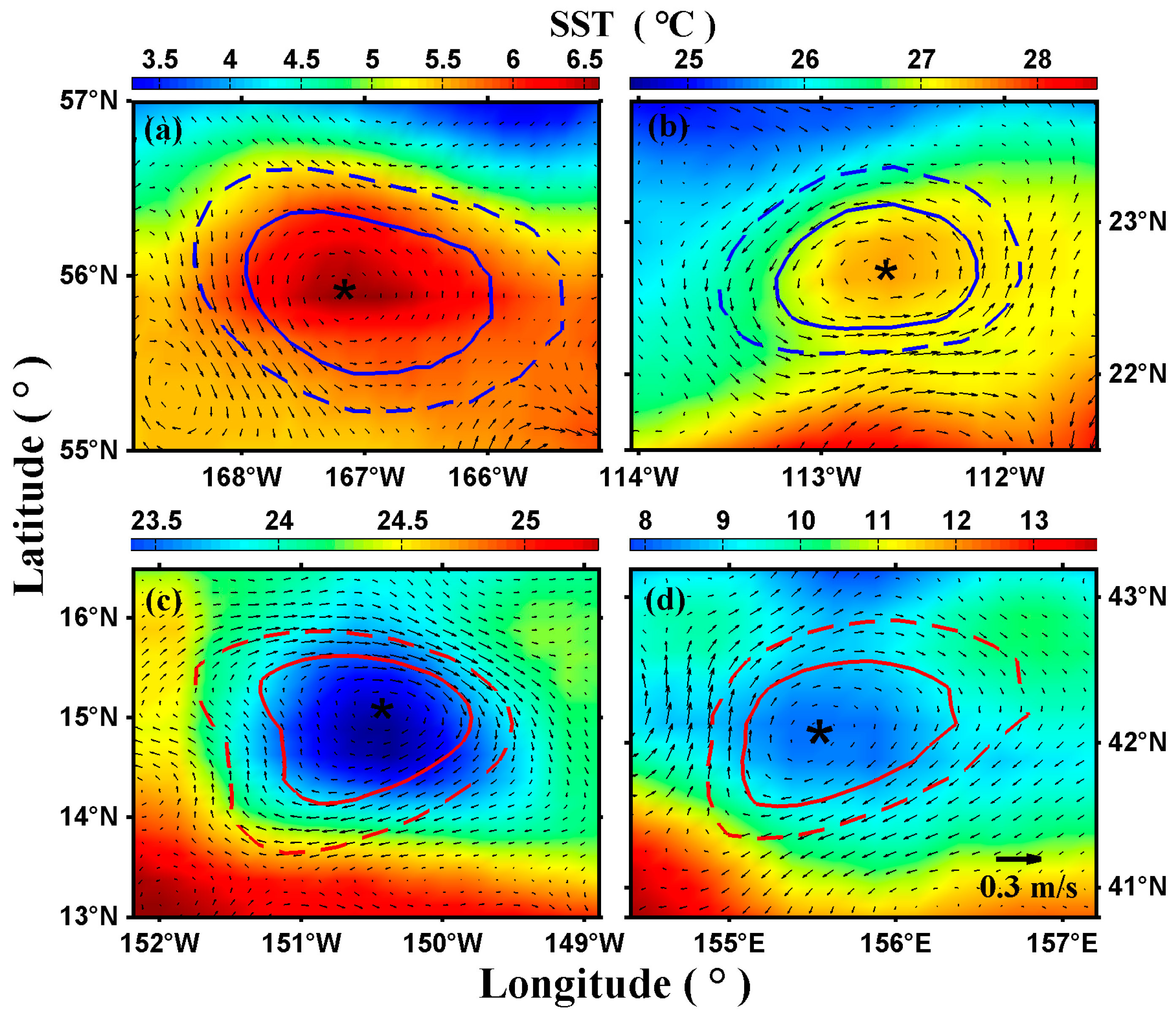
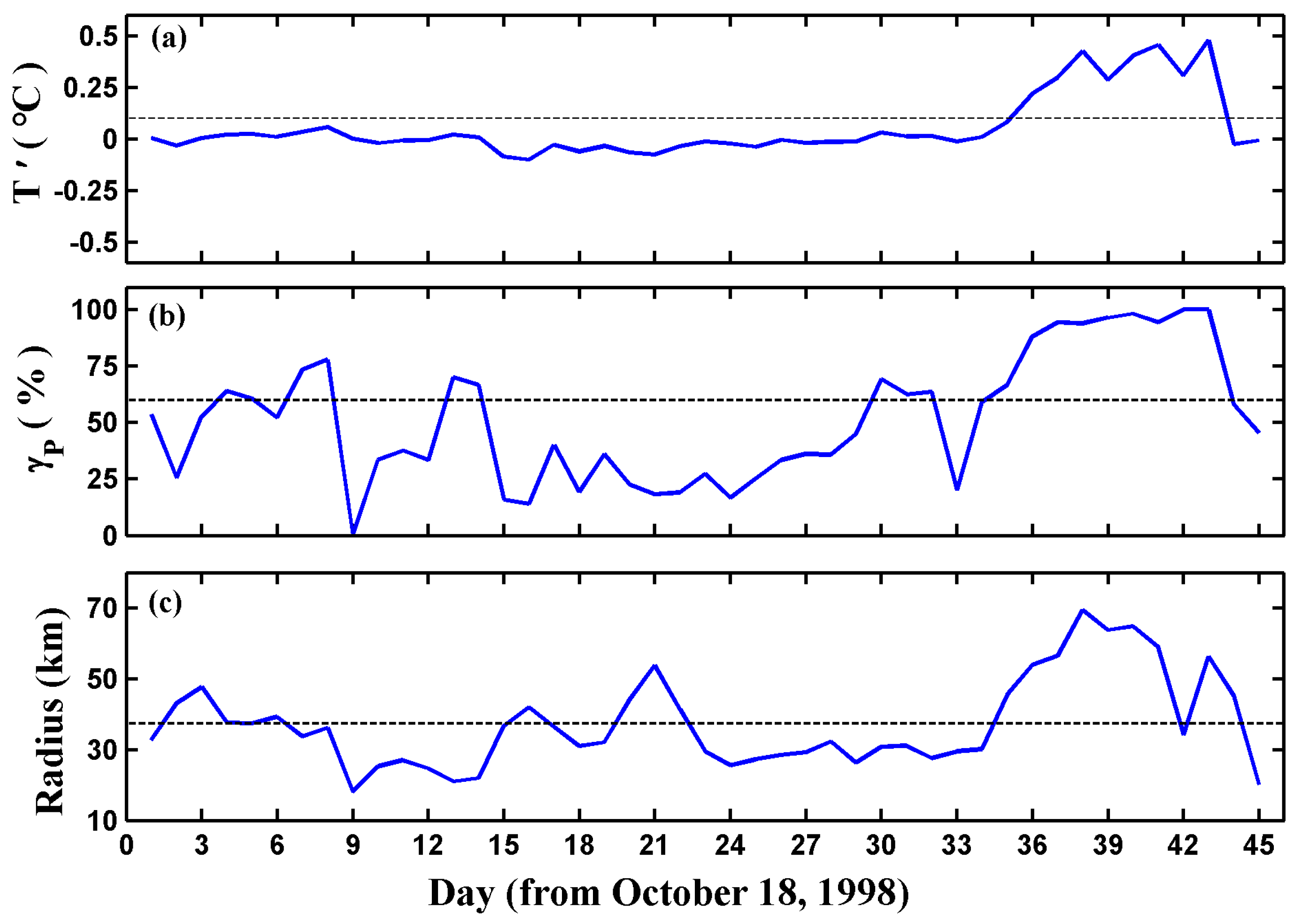
3.1. Cyclonic Warm-Core and Anticyclonic Cold-Core Eddy Cases

According to the definition of CW-ACE in this study, four cases (2 CWEs and 2 ACEs) are shown in Figure 2. The temperature at all the points within these CWE (ACE) cases is warmer (cooler) than the background mean temperature, i.e., γ p = 100% in all of the four cases.
Figure 2a displays day 43 of a CWE, which appeared on 1 December 1998. The eddy center is located at (167.125°W, 55.875°N), the mean radius is about 56.3 km, the amplitude (the maximum absolute value of SSHA) reaches 7.9 cm, and the maximum T reaches 0.48 °C. This eddy survived 45 days, and turned from “normal” cyclonic eddy to CWE on day 35. In the other case, the eddy appeared on 21 August 2010 (Figure 2b). For day 267, its center is located at (112.625°W, 22.625°N), the mean radius is about 52.5 km, the amplitude is 8.4 cm, and the maximum T reaches 0.42 °C. This eddy survived 281 days, and turned from “normal” cyclonic eddy to CWE on day 25.
Besides the CWEs, there are ACEs in the North Pacific as well. Figure 2c presents an ACE case occurring on 27 April 2001. Its center is located at (150.375°W, 15.125°N), the mean radius is about 82.5 km, the amplitude reaches 12.7 cm, and the maximum T is −0.54 °C. This eddy survived 92 days and turned from “normal” anticyclonic eddy to ACE on day 85, and the figure shows the eddy on day 87. The second ACE case emerges on 19 June 2005 (Figure 2d). Its center is located at (155.5°E, 42.0°N), the mean radius is about 55.5 km, the amplitude reaches 14.4 cm, and the maximum T is −0.77 °C. This eddy survived 105 days, and it turned from “normal” anticyclonic eddy to ACE on day 93. Figure 2d shows the eddy on day 99.
From the four cases, it seems that the CW-ACE can appear in different seasons and different subregions of the North Pacific. Therefore, it is necessary to systematically study the spatio-temporal characteristics and regional dependence of the CW-ACE. In the Discussion section, their generation mechanisms are introduced.

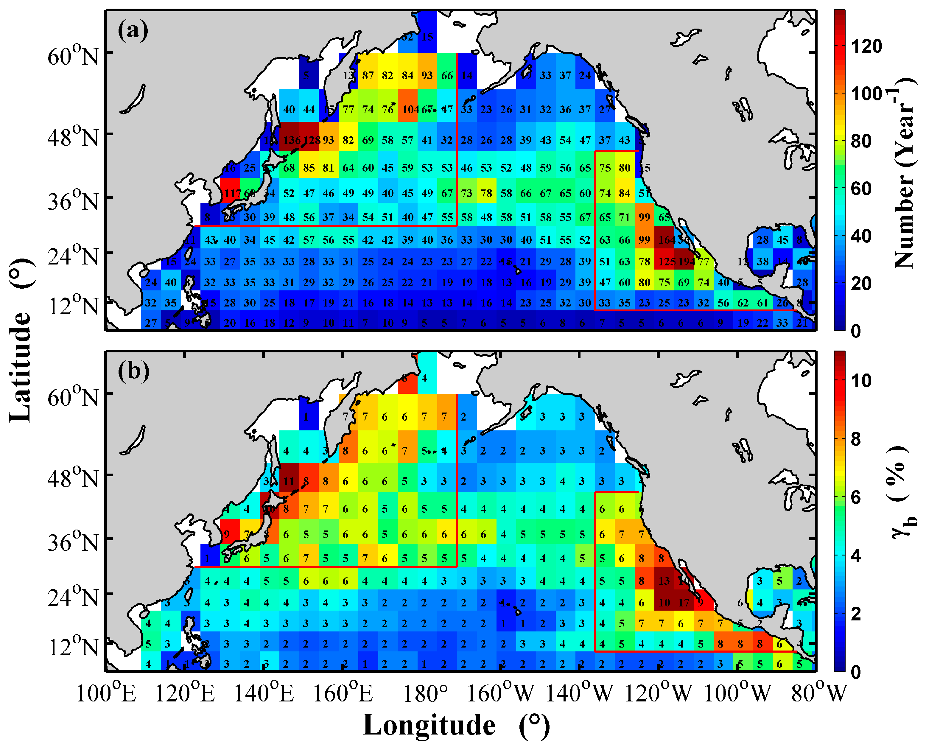
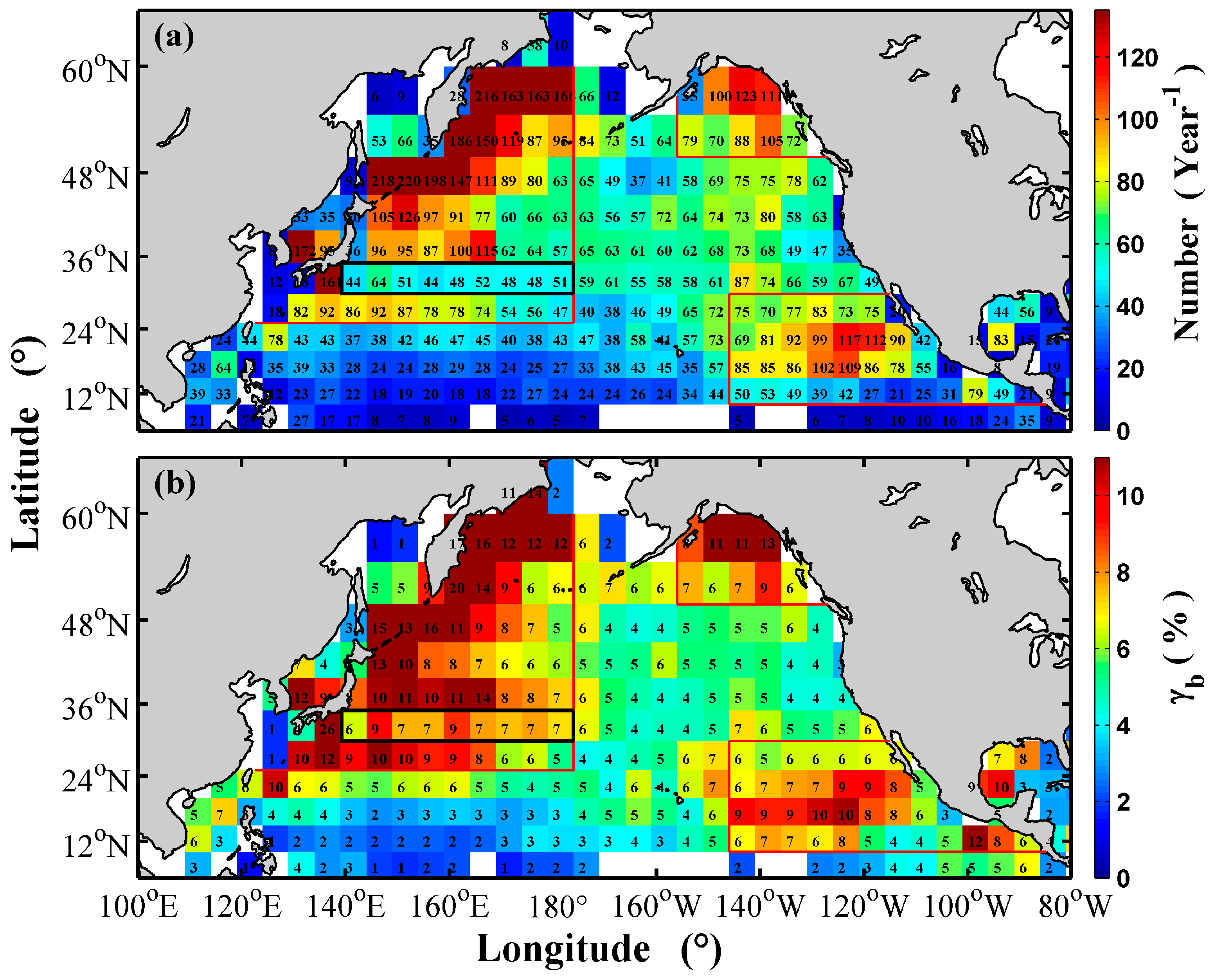
3.2. Spatial Distribution Characteristics

In order to illustrate the spatial distribution of the CW-ACEs, Figure 3 presents the annual mean number of the ACEs (Figure 3a) and their occurrence frequency ( γ b , Figure 3b) in each 5° by 5° bin; γ b is defined as the ratio of N a b n , b i n to N t o t , b i n , where N a b n , b i n is the number of the CW-ACEs and N t o t , b i n is the total number of the same polarity eddies within the target bin, i.e., γ b = N a b n , b i n N t o t , b i n × 100 % .
It is clearly observed that the CWEs are mostly concentrated in the northwest (north of 30°N and west of 170°W, mainly in the OC and the KE region) and southeast (north of 10°N, south of 45°N, and east of 135°W, mainly in the CC region) of the North Pacific. Although the CWEs exist in other area as well, the number and γ b are significantly smaller. In the CC region, the maximum number ( γ b ) reaches 194 (17%) per year, and the minimum number is only 5 (less than 1%) per year in the NEC region.
Similarly, the annual mean number of the ACEs and the associated occurrence frequency are shown in Figure 4. The ACEs are mainly concentrated in the northwest (north of 25°N, west of 180°, mainly in the OC and the KE region), southeast (10°N~30°N, east of 145°W, mainly in the CC region), and northeast (north of 50°N, east of 155°W, mainly in the AC region) of the North Pacific. The maximum number of the ACEs appears in the OC region (near the KE region, about 220 per year), and the highest γ b (about 26%) is located in the KE region.
Compared with the CWEs, (1) both the number and γ b of the ACEs are larger/higher in almost each 5° by 5° bin. (2) The AC region is active for the ACEs, but inactive for the CWEs. (3) The ACEs occur farther south (extending to about 30°N) in the KE region. (4) There is a significant zonal low-value band (the black solid rectangular region in Figure 4a,b) to the south of the KE axis (about 35°N) for the ACEs, while it is inconspicuous for the CWEs. (5) South of the North Pacific area, bins with no ACE values can be found, while no such blank bins are observed for the CWEs. This difference is due to the definition of the CW-ACE, more specifically the limit of T . If lower (higher) T is applied, then the blank bins will disappear (appear) for CWE and ACE.

3.3. General Characteristic of Cyclonic Warm-Core and Anticyclonic Cold-Core Eddy

3.3.1. Cyclonic Warm-Core and Anticyclonic Cold-Core Eddy Generation Time

The previous studies suggested that the CW-ACEs could be generated from “normal” eddies [55], and thus “When do ‘normal’ eddies turn to CW-ACEs?” is a rather interesting question. To address this question, Figure 5 gives the proportion of generation ratio ( γ g ) of the CW-ACEs in the different lifespan stages and the annual mean occurrence frequency of CW-ACEs ( γ s ) in these stages (Figure 5b). Here, γ g is defined as the ratio of N a b n , g e n e r a t i o n to N t o t , where N a b n , g e n e r a t i o n is the number of newly generated CW-ACEs in the target normalized lifespan stage and N t o t is the total number of cyclonic (anticyclonic) eddies, i.e., γ g = N a b n , g e n e r a t i o n N t o t × 100 % . The γ s is defined as the ratio of N a b n , s t a g e to N t o t , where N a b n , s t a g e is the number of CW-ACEs in the target normalized lifespan stage (not only the newly generated CW-ACEs in this stage but also include already existed eddies from former stages), i.e., γ s = N a b n , s t a g e N t o t × 100 % .
From Figure 5a, the CWEs (blue curve) mainly generate in the beginning stage and the decaying stage, while fewer CWEs generate in the mature stage. This characteristic may come from the eddy instability during the beginning and decaying stages, while it is more coherent in the mature stage. Liu et al. [76] pointed out that the eddy’s radius, vorticity, and shape almost do not change in the mature stage. This characteristic prevents the generation of the CW-ACEs (for more details, please refer to the Discussion section).
It is clearly seen that γ s of the CWEs (Figure 5b, blue curve) is high in the beginning and decaying stages, while low in the mature stage. This indicates that some CWEs generate in the beginning stage, but turn into “normal” eddies afterwards (at least no longer meet the definition of the CWE), which reduces the proportion in the mature stage. However, some new CWEs are generated in the decaying stage, thus increasing the proportion again.
On the contrary, the proportion of the ACEs keeps growing continually from 0.1~0.2 normalized lifespan stage until dissipation (Figure 5b, red curve). Therefore, once an ACE forms, it is harder for it to turn back to “normal” again. Besides, the “normal” anticyclonic eddies continue to transform into ACEs in the following stages, leading to a higher and higher proportion until the end. Such different evolutions may imply different generation mechanisms between the CWEs and ACEs. Further studies of the three-dimensional structure of CW-ACEs are therefore needed.

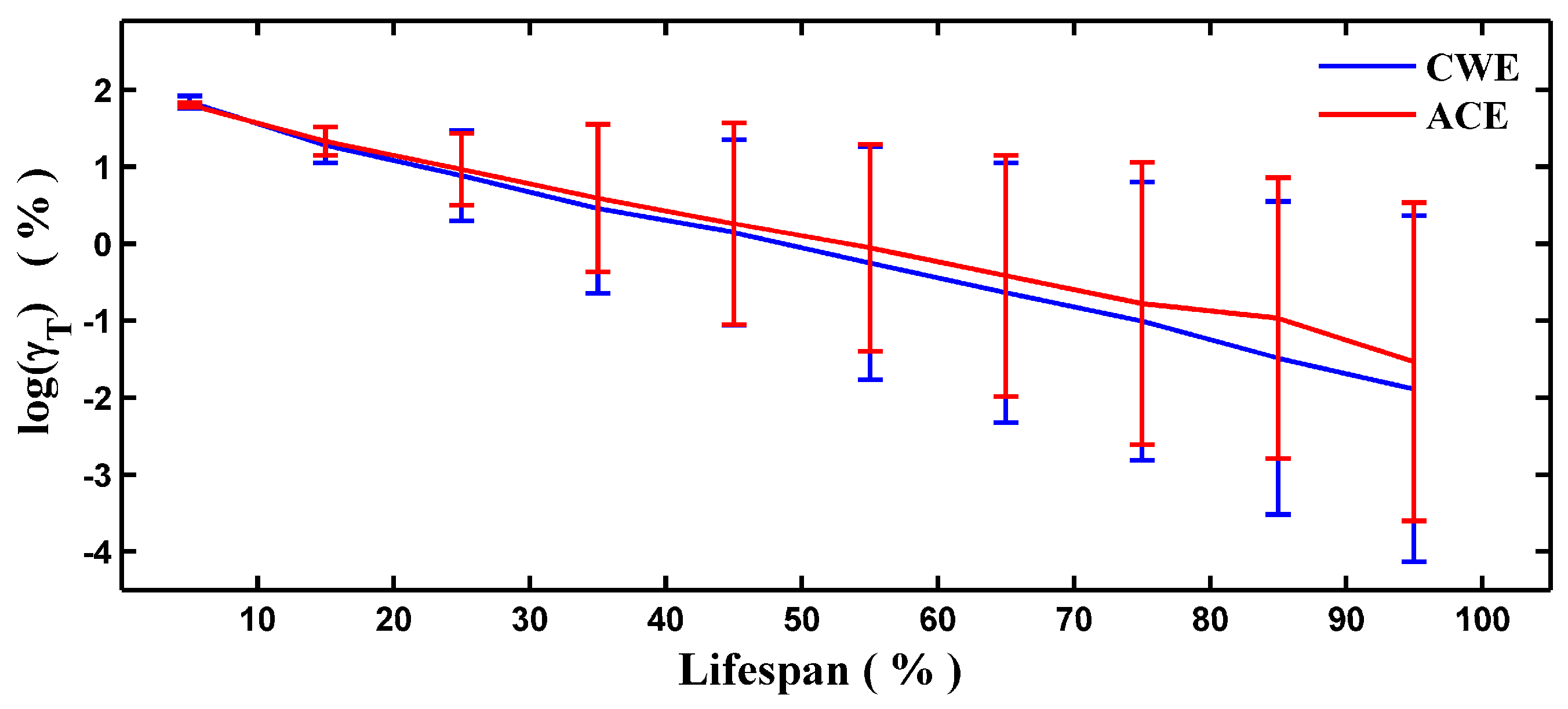
3.3.2. Cyclonic Warm-Core and Anticyclonic Cold-Core Eddy Survival Time

As in Figure 5 and the previous literature [55], the “normal” eddies can transform into CW-ACEs, and reverse back. In other words, CW-ACEs may only occupy some periods of the whole lifespan. Figure 6 gives the annual mean distribution of γ T , which is defined as the ratio of T a b n , s p a n to T t o t , where T a b n , s p a n is the time span during which the eddy is an CWE or ACE for each eddy track, and T t o t corresponds to the whole eddy lifespan, i.e., γ T = T a b n , s p a n T t o t × 100 % . In order to present the figure clearly, a logarithmic scale (base 10) for γ T is used along the y-axis. About (69.5 ± 0.8)% of the ACEs survives no longer than 10% of the whole lifespan, and only (1.3 ± 0.6) out of ten thousand persist longer than 90%. For the CWEs, the survival time of about (63.6 ± 1.1)% is no more than 10% of the whole lifespan, and only 2.9 ± 0.8 out of ten thousand CW-ACEs survive longer than 90%.

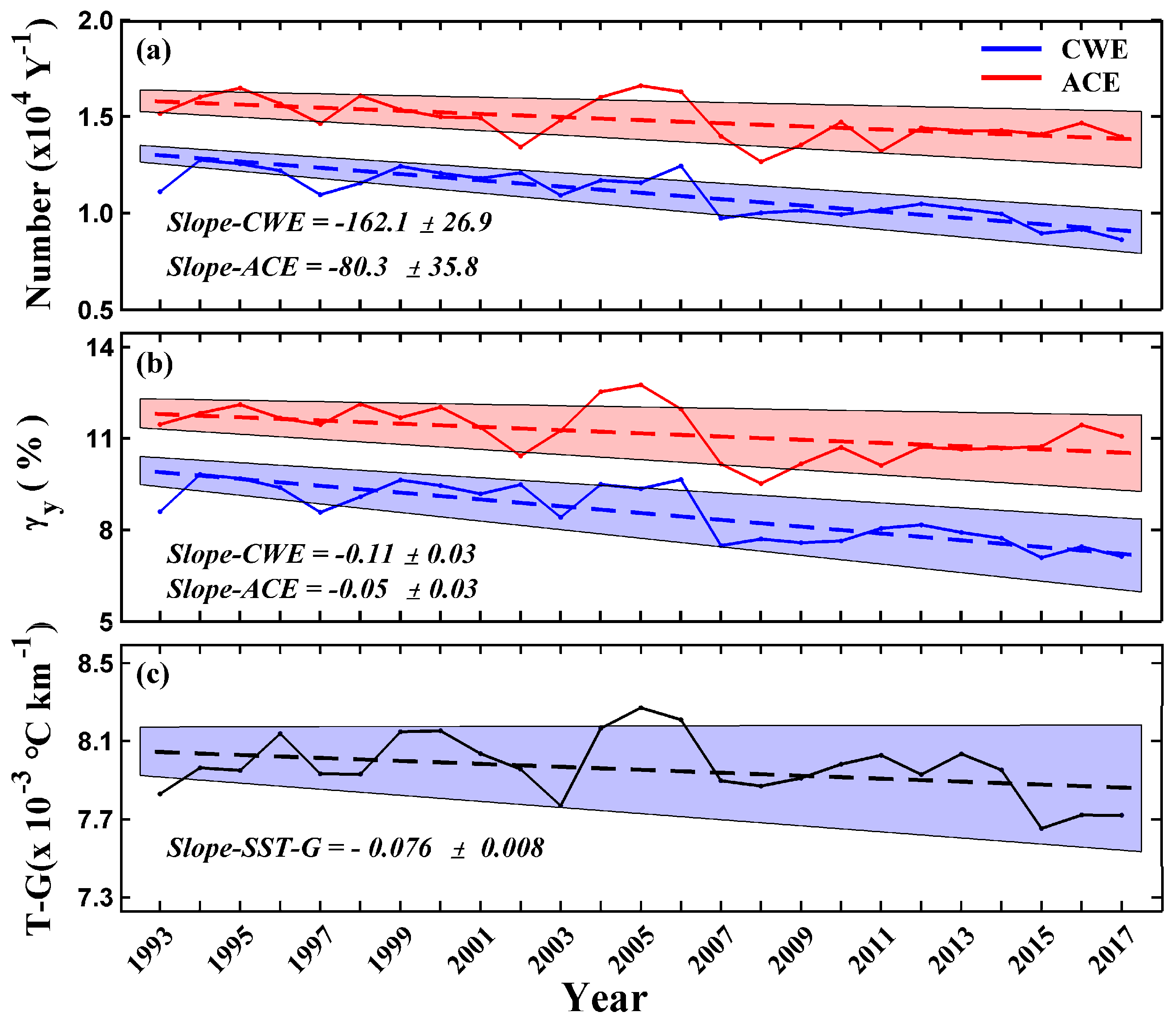
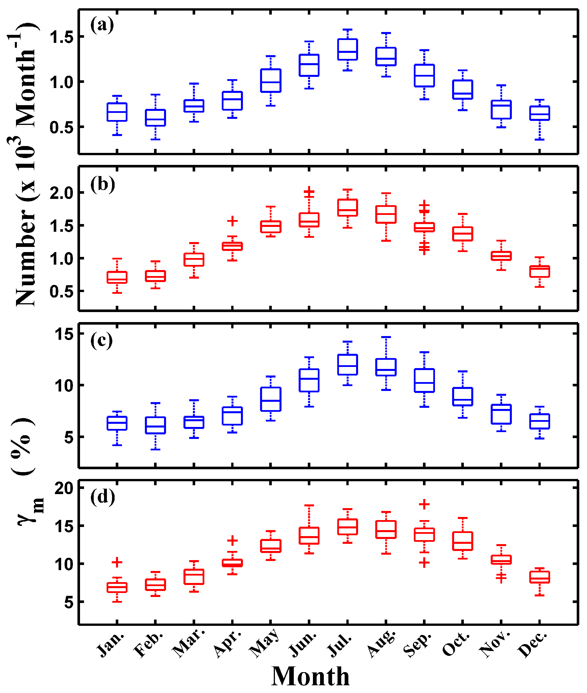
3.4. Inter-Annual and Seasonal Variation

In some respects, the number of CW-ACE indirectly reflect the mesoscale eddies activity. The time series of CW-ACE number and the associated occurrence frequency ( γ y ) are shown in Figure 7a,b, respectively; γ y is defined as the ratio of N a b n , y e a r to N t o t , y e a r , where N a b n , y e a r is the number of CWEs (ACEs) in the target year, and N t o t , y e a r is the total number of cyclonic (anticyclonic) eddies in the same year, i.e., γ y = N a b n , y e a r N t o t , y e a r × 100 % .
As a whole, the CW-ACE number and the associated occurrence frequency γ y show a decreasing pattern year by year. The linear decreasing rate of the CWEs (ACEs) number is −162.1 ± 26.9 (−80.3 ± 35.8) (Figure 7a, dashed line) per year. It means that the CWEs decay about twice as fast as the ACEs. The linear slope of γ y is −0.11 ± 0.03 for CWEs and −0.05 ± 0.03 for ACEs (Figure 7b, dashed line). Similarly, the decreasing rate of the CWEs occurrence frequency is about twice as fast as the ACEs.
As pointed out by Zhang et al. [26], the horizontal advection of eddy currents can lead to an asymmetric temperature anomaly dipole near the surface, whereas the vertical advection of upwelling and downwelling results in a temperature core at deeper levels in the large SST gradient area. In other words, the sea water temperature within eddies are determined by two reasons, the surrounding area sea water temperature and the eddy-induced vertical movement. Considering that the vertical distribution of the sea water temperature usually does not significantly change, this paper assume that the decreasing trend of the CW-ACEs may be caused by the SST gradient changes. Figure 7c gives the time series of the annual mean SST gradient, where a similar variation trend to the CW-ACEs decreasing pattern is observed. The linear decreasing rate of the SST gradient is ( 0.076 ± 0.008 ) × 10 3 °C per year. The correlation coefficients between the SST gradient curve and CWE, ACE, and CW-ACE curves are 0.69, 0.54, and 0.68, respectively, and are all statistically significant on the 90% confidence level. This means the SST gradient changes can be considered as the main reason for the CW-ACEs decreasing trend.
The number of CW-ACEs and the corresponding occurrence frequency ( γ s e ) show significant seasonal variation (Table 1). Here, γ s e is defined as the ratio of N a b n , s e a s o n to N t o t , s e a s o n , where N a b n , s e a s o n is the number of the CWEs (ACEs) appearing in the target season, and N t o t , s e a s o n is the total number of the cyclonic (anticyclonic) eddies in the same season, i.e., γ s e = N a b n , s e a s o n N t o t , s e a s o n × 100 % . The CW-ACEs are active in summer (June, July, August), while inactive in winter (December, January, February). The maximum number ( γ s e ) of CWEs is in summer, up to 3618.6 ± 357.8 ((11.43 ± 1.11)%), and the minimum number ( γ s e ) is only 1896.6 ± 311.6 ((6.28 ± 0.87)%) in winter. Correspondingly, for the ACEs, the maximum and minimum number ( γ s e ) are 5029.4 ± 480.1 ((14.37 ± 1.23)%) and 2231.4 ± 275.9 ((7.39 ± 0.80)%), appearing in summer and winter, respectively.
In order to show the seasonal variation clearly, the climatological monthly number, and the associated occurrence frequency ( γ m ) of the CW-ACEs are displayed in Figure 8. Similarly, γ m is defined as the ratio of N a b n , m o n t h to N t o t , m o n t h , where N a b n , m o n t h is the number of the CWEs (ACEs) appearing in the target month, and N t o t , m o n t h is the total number of the cyclonic (anticyclonic) eddies in the same month, i.e., γ m = N a b n , m o n t h N t o t , m o n t h × 100 % . The CWEs are the most active in July, with a maximum number ( γ m ) up to 1355.7 ± 26.6 ((12.1 ± 0.24) %), while they are the most inactive in February, with a minimum number ( γ m ) of only 603.9 ± 26.3 ((6.1 ± 0.23) %). Likewise, for the ACEs, the maximum number ( γ m ) is also in July, reaching 1757.4 ± 32.4 ((14.9 ± 0.25) %), and the minimum monthly mean number ( γ m ) is only 702.8 ± 24.4 ((6.9 ± 0.22) %) in January.

3.5. The Regional Dependence

The ocean currents are complex in the North Pacific (Figure 1), thus seven subregions are defined (Appendix A) to investigate the detailed feature of the CW-ACEs [69]. The mean radius, temperature anomalies, EKE, and amplitude of the CW-ACEs all have large standard deviations (Table 2), indicating less homogeneity. Thus, composite analysis cannot be used to compare the characteristics in the different subregions. Therefore, the boxplots of the CW-ACEs characteristics within the 25 % to 75 % are used to compare the differences in the seven subregions (Figure 9).
The mean radius of the CW-ACEs varies in the different subregions (Figure 9a), and decreases with the increasing latitude. The CW-ACEs with the smallest radius appear in the OC region, while those with the largest radius are in the NEC region. This may be associated with the baroclinic Rossby deformation radius changing with latitude. Besides, the absolute value of the maximum temperature difference ( | T | , Figure 9b) could be regarded as another indicator of the CW-ACEs activity. The largest | T | appears in the KE region, and the smallest | T | is in the NEC region. Correspondingly, the KE region is the strongest subregion of the CW-ACEs activity in the North Pacific.
EKE is considered as the third indicator to measure the CW-ACEs activity (Figure 9c). The EKE is highest in the KE region (especially for the CWEs), where it is several times higher than that in the AC region. The amplitude of the CW-ACEs, considered as the fourth indicator, is shown in Figure 9d. Similar to EKE, the largest and smallest amplitude also appear in the KE and AC region, respectively. To sum up, the KE region is the strongest subregion of the CW-ACEs activity in the North Pacific, in terms of the CW-ACE-induced temperature change, EKE, and amplitude.

4. Discussion

As presented in this study, CW-ACEs are widely distributed in the North Pacific, according to the definition. In order to deepen the understanding of this phenomenon, the cases of CW-ACEs from Figure 2a,d are chosen to discuss the generation mechanisms. As noted in Section 3, this eddy survived for 45 days, and appeared as a CWE from day 35 to day 43 (Figure 10). At the transition stage (i.e., day 35), the eddy’s T , γ p , and radius increase sharply. One possible theory is that the eddy loses its strong coherent structure and becomes very unstable when reaching the decaying stage [76]. The eddy studied in this paper did appear that its radius suddenly increases when turning into CWE, and absorbs warm sea waters from the surrounding area, which in turn changes the water property within the eddy.
In order to support this assumption, Figure 11 gives the evolution of the SST and eddy boundary during before and after the transition time (day 35, i.e., 23 November 1998). It is clear that this eddy in Figure 11a is a “normal” eddy before the transition. The temperature in the surrounding area is generally lower to the west and north of the eddy and higher to the east. Compared with Figure 11a, the temperature of the sea water within the background area is rising over the period of observation, and this rising ambient temperature offers the chance to generate the CWE. On 24 November 1998 (Figure 11c), the eddy radius suddenly increases, while it absorbs warm sea waters from the surrounding area, and then turns to a CWE. Figure 11d shows the “first day” after it has turned into a CWE (25 November 1998). The eddy radius continues increasing and it moves to the north (the colder water area). This makes the mean temperature in the area surrounding the eddy decrease, and as a result, T increases. In short, at the decaying stage, the “normal” eddy radius suddenly increases and it absorbs warm sea waters from the surrounding area, and then turns into a CWE. Subsequently, the eddy moves to the colder water area and gets even stronger.
Besides the CWE discussed above, the ACE depicted in Figure 2d is chosen to show its generation mechanism. Temporal evolution of T , γ p , and radius for the ACW is given in Figure 12. Similar to the CWE depicted in Figure 10, the transition to ACE occurs in the final “decaying” stage. T and γ p have changed significantly during the transition process. However, the radius have not changed much then. This fact indicates that the generation mechanism of ACE is different from that of CWE. In other words, this transition to ACE is unlikely a result of its increased instability during its “decaying” stage.
The sea conditions (temperature and current) of the area surrounding the ACE are given in Figure 13, for the period in which the transition into ACE occurs (11–14 June 2005), in an attempt to study its generation mechanism. Figure 13a,b are for the “normal” eddy, whereas Figure 13c,d are for the ACE. Figure 13a clearly shows that water to the north of the “normal” eddy is cold. There is another cyclonic eddy to the west, and a water mass of higher temperature exists between these two eddies. This warm water mass is dragged to the surroundings of the normal anticyclonic eddy by the strong current associated with sheared eddy. The cold water to the north is entrained into the interior of the eddy. As shown in Figure 13c, the water surrounding the anticyclonic eddy is warmed by the eddy strong shear processes, helping the transition from “normal” eddy to ACE. On the first day after the ACE’s formation, the warm water mass is almost homogeneously distributed around the ACE, while the cold water from the north is entrained into the ACE interior, strengthening the ACE itself. In summary, it appears that the formation of this ACE is unlikely to be linked to instability. Rather, the interaction between adjacent eddies seem to have played an important role. It is this eddy-eddy interaction that transports warm water into the surrounding area and entrains the cold water into the ACE interior.
The generation mechanisms for CW-ACEs are discussed by studying one specific case for each kind of eddy. The two possible mechanisms found here are instability during the decay stage and eddy horizontal entrainment. The former mechanism is characterized with a sharp change in eddy radius, while in the latter case, little change in eddy radius is found. Other mechanisms, as discussed in the Introduction section, cannot be ruled out of course. The generation mechanism of CW-ACEs is still a very interesting scientific question. It appears insufficient to study this problem using only surface data, as the surface data can only reflect the surface conditions of oceanic eddies, while the information of the interior is absent. Further studies using 3-D observational data or numerical models are on the way.

5. Conclusions

The phenomenon of CW-ACEs is observed in the North Pacific. Following the definition of CW-ACEs presented in this study, this paper reveals the spatial distribution of the CW-ACEs in each 5° by 5° bin. The statistics indicate that the CWEs are mainly concentrated in the northwest and southeast of the North Pacific. Besides these two regions, the ACEs are also concentrated in the northeastern area. The highest γ b reaches 17% for the CWEs, appearing in the CC region, and 26% for the ACEs, appearing in the KE region.
The occurrence frequency ( γ s ) of the ACEs is higher in the beginning and decaying stages, while lower in the mature stage. However, the occurrence frequency of the ACEs grow almost linearly in 0.1–0.9 stages. It is also found that about (69.5 ± 0.8)% of the CWEs and (63.6 ± 1.1)% of the ACEs survive shorter than 10% of the whole eddy lifespan. Only 1.3 ± 0.6 out of ten thousand eddies for the CWEs and 2.9 ± 0.8 out of ten thousand eddies for the CWEs survive longer than 90% of the whole eddy lifespan. Therefore, most of the CW-ACEs are short-term phenomena and cannot survive for a long time like the “normal” eddies.
The annual mean number and the associated occurrence frequency ( γ y ) decrease year by year for CW-ACEs, and the decreasing rate of the CWEs is almost twice as fast as that of the ACEs. The number of CW-ACEs ( γ y ) reduces by about 162.1 ± 26.9 ((0.11 ± 0.03)%) each year for the CWEs, and about 80.3 ± 35.8 ((0.05 ± 0.03)%) for the ACEs. This decreasing trend is due to the SST gradient decreasing pattern. The CW-ACEs have a significant seasonal variation, being intense in summer and weak in winter. The maximum number ( γ m ) of the CWEs appears in July, and the minimum number ( γ m ) appears in February. The maximum number ( γ m ) of the ACEs also appears in July, while the minimum number ( γ m ) appears in January.
In view of the complex ocean currents and different dynamic environment, the North Pacific is divided into seven subregions, and the dynamic properties of the CW-ACEs (the mean radius, T , EKE, and amplitude) are discussed in each subregion. The KE region is the most active area of the CW-ACEs from the perspective of the CW-ACE-induced T , EKE, and amplitude.
In addition, generation mechanisms for CW-ACEs are discussed. The two possible mechanisms found here are (1) instability during the decay stage and (2) eddy-eddy interaction and horizontal entrainment. This study, though not exhaustive, paves the road to study CW-ACE generation mechanisms using three-dimensional data.
The statistical analysis of the CW-ACEs contributes to a comprehensive understanding of the mesoscale eddy activity, and it is beneficial to the selection of the buoy sites in the future. The analysis of the dynamic characteristics in the different subregions is conductive to comprehend the CW-ACEs activity in different environments. Although only sea surface remote sensing data is applied in this paper, it could be a foundation for further study about the three-dimensional structure and generation mechanisms of the CW-ACEs.

Author Contributions

Writing—original draft, C.D., W.T., and Y.H.; writing—review and editing, W.S.

Funding

This research was funded by the National Key Research and Development Program of China (2017YFA0604100), the National Key Research Programs of China (2016YFA0601803), the National Programme on Global Change and Air-Sea Interaction (GASI-03-IPOVAI-05), the National Natural Science Foundation of China (41806039, 41476022, 41490640), the Program for Innovation Research and Entrepreneurship Team in Jiangsu Province, the foundation of China Ocean Mineral Resources R&D Association (DY135-E2-2-02, DY135-E2-3-01), the Priority Academic Program Development of Jiangsu Higher Education Institutions (PAPD), the Natural Science Foundation of Jiangsu Province (BK20150912), and the Natural Science Foundation of Jiangsu Higher Education Institutions of China (16KJB170011), the China Postdoctoral Science Foundation (2018M640501) and Jiangsu Province Postdoctoral Foundation grant.

Acknowledgments

The altimeter products are produced by the Ssalto/Duacs and distributed by AVISO, with support from the CNES (http://www.aviso.oceanobs.com/duacs/). The AVHRR SST product data were obtained from the NASA JPL Web site. The authors are thankful to Kenny T.C. Lim Kam Sian and Dong Wang for proofreading and providing constructive comments, which improved the overall English level of the paper. We thank the editor and four anonymous reviewers for their constructive comments and helpful suggestions on an earlier version of the manuscript.

Conflicts of Interest

The authors declare no conflict of interest.

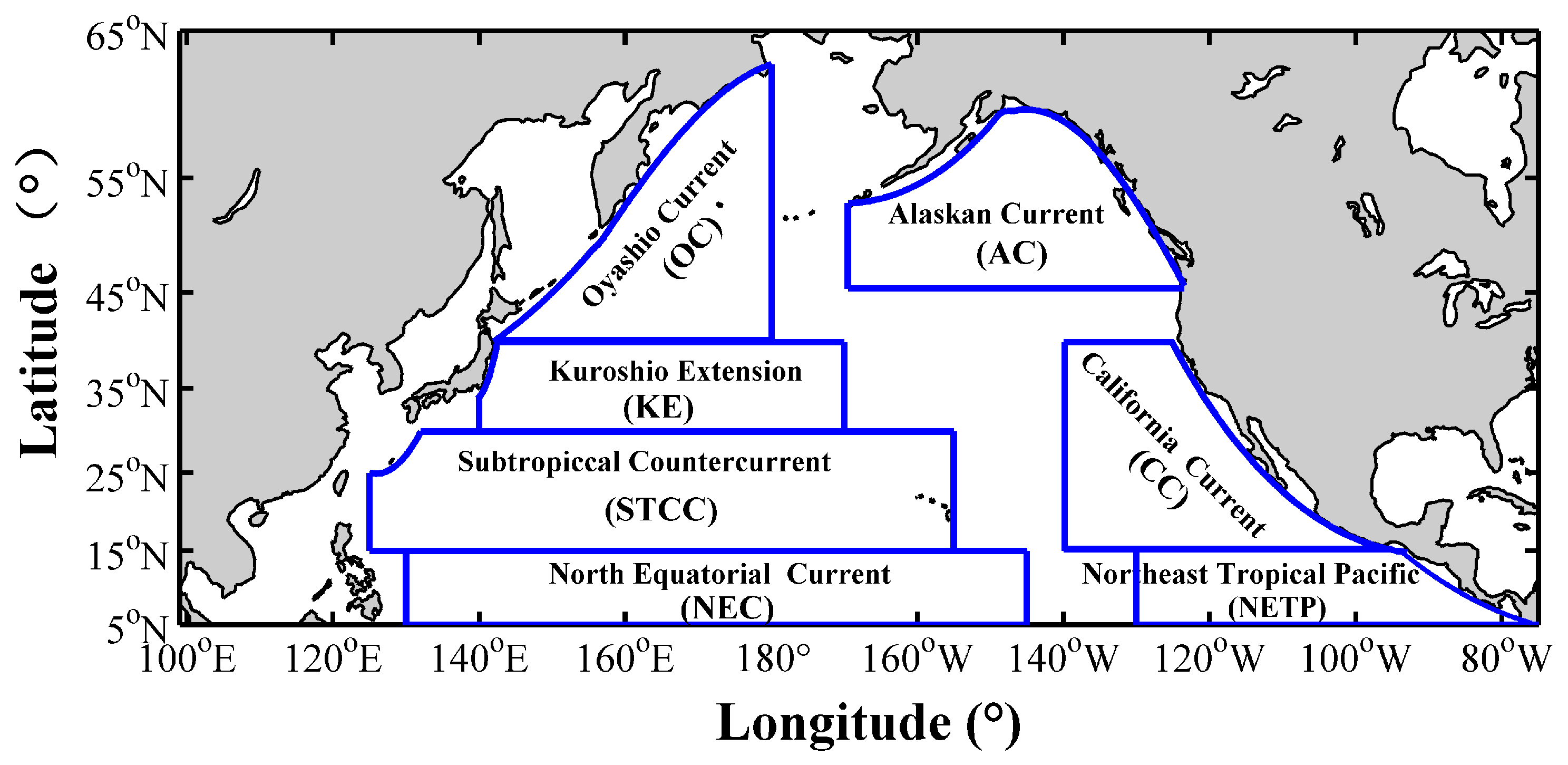
Appendix A: Subregions in the North Pacific

The detailed range of the seven subregions in the North Pacific (Figure A1) are as follows:
(1) North Equatorial Current (NEC) region: a rectangular region, (130°E~145°W, 5°N~15°N);
(2) Subtropical Countercurrent (STCC) region: an approximately rectangular region, about (125°E~155°W, 15°N~30°N);
(3) Kuroshio Extension (KE) region: an approximately rectangular region, about (140°E~170°W, 30°N~40°N);
(4) Oyashio Current (OC) region: an approximately triangular region, about (140°E~180°, 40°N~62°N);
(5) Northeast Tropical Pacific (NETP) region: an approximately trapezoidal region, about (130°W~80°W, 5°N~15°N);
(6) California Current (CC) region: an approximately trapezoidal region, about (140°W~100°W, 15°N~40°N);
(7) Alaska Current (AC) region: an approximately fan-shaped region, about (170°W~120°W, 45°N~60°N).
Figure A1. Location of the seven subregions in the North Pacific.
Remotesensing 11 00208 g0a1

Appendix B: Eddy Detection Scheme

In brief, the eddy detection and tracking method includes three steps: (1) determine the eddy center, (2) extract the eddy boundary, and (3) track the eddy lifespan.
Step one, determine the eddy center satisfying the following constraints:
(1) The zonal component of the geostrophic velocity anomaly ( u ) must change its sign along a meridional section across the eddy center, and its magnitude must increase within the range of a (parameter) pointing away from the eddy center in both northward and southward directions.
(2) Similar to the condition (1), the meridional component of geostrophic velocity anomaly ( v ) must change its sign along an zonal section across the eddy center, and its magnitude must increase within the range of a pointing away from the eddy center in both eastward and westward directions.
(3) Eddy center is featured by a locally minimum magnitude of the geostrophic velocity anomaly ( u 2 + v 2 ) within the region that extends by b (parameter) grid pointing around this center.
(4) If the eddy center is chosen as the original point to construct a local Cartesian coordinate, then the direction of the geostrophic velocity anomaly ( u , v ) should follow the same direction of rotation. In other words, the geostrophic velocity anomaly vector forms the clockwise or anticlockwise local flow.
Step two, extract the eddy boundary which is defined as the outermost enclosed contour of the local stream function around the eddy center.
Step three, the eddy tracking method used in this paper is similar to Doglioli et al. [82] and Chaigneau et al. [83]. If an eddy is successfully detected at the time step t , then the same polarity eddy (cyclonic or anticyclonic) is searched for at the next time step t + 1 within a searching area (i.e., a circular region with a 1.2° radius and its center coinciding with the eddy center). Choose the nearest one that is well-defined, if there is more than one eddy satisfying the condition. On the contrary, if there is no eddy found at time step t + 1 , a second search will be taken at time step t + 2 within an extended searching area (1.5 times the radius of the searching area). If there is still no eddy satisfying the requirement, this eddy will be considered as ‘‘decayed’’, then the eddy’s lifespan is defined as the time from the first successful detection to this time step. Two parameters required in this method are chosen as a = 3 and b = 2 in this study. For more details about this tracking method, please refer to Nencioli et al. [72].

References

  1. Chelton, D.B.; Schlax, M.G.; Samelson, R.M.; Szoeke, R.A. Global observations of large oceanic eddies. Geophys. Res. Lett. 2007, 34. [Google Scholar] [CrossRef] [Green Version]
  2. Chelton, D.B.; Schlax, M.G.; Samelson, R.M. Global observations of non-linear mesoscale eddies. Prog. Oceanogr. 2011, 91, 167–216. [Google Scholar] [CrossRef]
  3. Morrow, R.; LeTraon, P.Y. Recent advances in observing mesoscale ocean dynamics with satellite altimetry. Adv. Space Res. 2012, 50, 1062–1076. [Google Scholar] [CrossRef]
  4. Frenger, I.; Münnich, M.; Gruber, N.; Knutti, R. Southern Ocean eddy phenomenology. J. Geophys. Res. 2016, 120, 7413–7449. [Google Scholar] [CrossRef]
  5. Zhang, Z.; Wang, W.; Qiu, B. Oceanic mass transport by mesoscale eddies. Science 2014, 345, 322–324. [Google Scholar] [CrossRef] [PubMed]
  6. Yang, G.; Yu, W.; Yuan, Y.; Zhao, X.; Wang, F.; Chen, G.; Liu, L.; Duan, Y. Characteristics, vertical structures, and heat/salt transports of mesoscale eddies in the southeastern tropical Indian Ocean. J. Geophys. Res. 2015, 120, 6733–6750. [Google Scholar] [CrossRef] [Green Version]
  7. Pegliasco, C.; Chaigneau, A.; Morrow, R. Main eddy vertical structures observed in the four major Eastern Boundary Upwelling Systems. J. Geophys. Res. 2015, 120, 6008–6033. [Google Scholar] [CrossRef] [Green Version]
  8. Zhang, Z.; Zhang, Y.; Wang, W. Three-compartment structure of subsurface-intensified mesoscale eddies in the ocean. J. Geophys. Res. 2017, 122, 1653–1664. [Google Scholar] [CrossRef]
  9. He, Q.; Zhan, H.; Cai, S.; He, Y.; Huang, G.; Zhan, W. A new assessment of mesoscale eddies in the South China Sea: Surface features, three-dimensional structures, and thermohaline transports. J. Geophys. Res. 2018, 123, 4906–4929. [Google Scholar] [CrossRef]
  10. Qiu, B.; Chen, S. Eddy-induced heat transport in the subtropical north pacific from Argo, TMI and altimetry measurements. J. Phys. Oceanogr. 2004, 68, 458–473. [Google Scholar] [CrossRef]
  11. Meijers, A.J.; Bindoff, N.L.; Roberts, J.L. On the total, mean, and eddy heat and freshwater transports in the southern hemisphere of a global ocean model. J. Phys. Oceanogr. 2007, 37, 277–295. [Google Scholar] [CrossRef]
  12. Chen, G.; Gan, J.; Xie, Q.; Chu, X.; Wang, D.; Hou, Y. Eddy heat and salt transports in the South China Sea and their seasonal modulations. J. Geophys. Res. 2012, 117, 78–91. [Google Scholar] [CrossRef]
  13. Treguier, A.M.; Deshayes, J.; Lique, C.; Dussin, R.; Molines, J.M. Eddy contributions to the meridional transport of salt in the North Atlantic. J. Geophys. Res. 2012, 117. [Google Scholar] [CrossRef] [Green Version]
  14. Wang, X.; Wu, L.; Qi, Y.; Han, G. Heat, salt and volume transports by eddies in the vicinity of the Luzon Strait. Deep Sea Res. 2012, 61, 21–33. [Google Scholar] [CrossRef] [Green Version]
  15. Dong, C.; Mcwilliams, J.C.; Liu, Y.; Chen, D. Global heat and salt transports by eddy movement. Nat. Commun. 2014, 5, 1–6. [Google Scholar] [CrossRef] [PubMed]
  16. Xu, L.; Li, P.; Xie, S.P.; Liu, Q.; Liu, C.; Gao, W. Observing mesoscale eddy effects on mode-water subduction and transport in the North Pacific. Nat. Commun. 2015, 7, 10505. [Google Scholar] [CrossRef] [PubMed]
  17. Ma, X.; Jing, Z.; Chang, P.; Liu, X.; Montuoro, R.; Small, R.J.; Bryan, F.O.; Greatbatch, R.J.; Brandt, P.; Wu, D.; et al. Western boundary currents regulated by interaction between ocean eddies and the atmosphere. Nature 2016, 535, 533–537. [Google Scholar] [CrossRef]
  18. Kamidaira, Y.; Uchiyama, Y.; Mitarai, S. Eddy-induced transport of the Kuroshio warm water around the Ryukyu Islands in the East China Sea. Cont. Shelf Res. 2017, 143, 206–218. [Google Scholar] [CrossRef]
  19. Dong, D.; Brandt, P.; Chang, P.; Schütte, F.; Yang, X.; Yan, J.; Zeng, J. Mesoscale eddies in the Northwestern Pacific Ocean: Three-dimensional eddy structures and heat/salt transports. J. Geophys. Res. 2017, 122, 9795–9813. [Google Scholar] [CrossRef]
  20. Nurser, A.; Zhang, J. Eddy-induced mixed layer shallowing and mixed layer/thermocline exchange. J. Geophys. Res. 2000, 105, 21851–21868. [Google Scholar] [CrossRef] [Green Version]
  21. Martin, A.P.; Richards, K.J. Mechanisms for vertical nutrient transport within a North Atlantic mesoscale eddy. Deep Sea Res. 2001, 48, 757–773. [Google Scholar] [CrossRef]
  22. Kahru, M.; Mitchell, B.G.; Gille, S.T.; Hewes, C.D.; Holm Hansen, O. Eddies enhance biological production in the Weddell-Scotia Confluence of the Southern Ocean. Geophys. Res. Lett. 2007, 34, 116–130. [Google Scholar] [CrossRef]
  23. Klein, P.; Lapeyre, G. The oceanic vertical pump induced by mesoscale and submesoscale turbulence. Ann. Rev. Mar. Sci. 2009, 1, 351–375. [Google Scholar] [CrossRef] [PubMed]
  24. Kouketsu, S.; Tomita, H.; Oka, E.; Hosoda, S.; Kobayashi, T.; Sato, K. The role of mesoscale eddies in mixed layer deepening and mode water formation in the western North Pacific. J. Oceanogr. 2012, 68, 63–77. [Google Scholar] [CrossRef]
  25. Gaube, P.; Chelton, D.B.; Samelson, R.M.; Schlax, M.G.; O’Neill, L.W. Satellite observations of mesoscale eddy-induced Ekman pumping. J. Phys. Oceanogr. 2015, 45, 104–132. [Google Scholar] [CrossRef]
  26. Zhang, W.; Xue, H.; Chai, F.; Ni, Q. Dynamical processes within an anticyclonic eddy revealed from Argo floats. Geophys. Res. Lett. 2015, 42, 2342–2350. [Google Scholar] [CrossRef] [Green Version]
  27. Luneva, M.V.; Clayson, C.A.; Dubovikov, M.S. Effects of mesoscale eddies in the active mixed layer: Test of the parametrisation in eddy resolving simulations. Geophys. Astrophys. Fluid Dyn. 2015, 109, 1–30. [Google Scholar] [CrossRef]
  28. Bracco, A.; Clayton, S.; Pasquero, C. Horizontal advection, diffusion, and plankton spectra at the sea surface. J. Geophys. Res. 2009, 114, C02001. [Google Scholar] [CrossRef]
  29. Gruber, N.; Lachkar, Z.; Frenzel, H.; Marchesiello, P.; Münnich, M.; McWilliams, J.C.; Nagai, T.; Plattner, G. Eddy-induced reduction of biological production in eastern boundary upwelling systems. Nat. Geosci. 2011, 4, 787–792. [Google Scholar] [CrossRef]
  30. Chelton, D.B.; Peter, G.; Schlax, M.G.; Early, J.J.; Samelson, R.M. The influence of nonlinear mesoscale eddies on near-surface oceanic chlorophyll. Science 2011, 334, 328–332. [Google Scholar] [CrossRef]
  31. Mahadevan, A.; Asaro, E.D.; Lee, C.; Perry, M.J. Eddy-driven stratification initiates North Atlantic spring phytoplankton blooms. Science 2012, 337, 54–58. [Google Scholar] [CrossRef]
  32. Gaube, P.; Chelton, D.B.; Strutton, P.G.; Behrenfeld, M.J. Satellite observations of chlorophyll, phytoplankton biomass, and Ekman pumping in nonlinear mesoscale eddies. J. Geophys. Res. 2013, 118, 6349–6370. [Google Scholar] [CrossRef] [Green Version]
  33. Dufour, C.O.; Griffies, S.M.; de Souza, G.F.; Frenger, I.; Morrison, A.K.; Palter, J.B.; Sarmiento, J.L.; Galbraith, E.D.; Dunne, J.P.; Anderson, W.G. Role of mesoscale eddies in cross-frontal transport of heat and biogeochemical tracers in the Southern Ocean. J. Phys. Oceanogr. 2015, 45, 3057–3081. [Google Scholar] [CrossRef]
  34. Mahadevan, A. The impact of submesoscale physical on primary productivity of plankton. Ann. Rev. Mar. Sci. 2016, 8, 161–184. [Google Scholar] [CrossRef] [PubMed]
  35. McGillicuddy, D.J. Mechanisms of physical-biological-biogeochemical interaction at the oceanic mesoscale. Ann. Rev. Mar. Sci. 2016, 8, 125–159. [Google Scholar] [CrossRef] [PubMed]
  36. Brannigan, L. Intense submesoscale upwelling in anticyclonic eddies. Geophys. Res. Lett. 2016, 43, 3360–3369. [Google Scholar] [CrossRef] [Green Version]
  37. Frenger, I.; Münnich, M.; Gruber, N. Imprint of Southern Ocean eddies on chlorophyll. Biogeosciences 2018, 15, 4781–4798. [Google Scholar] [CrossRef]
  38. Lu, J.; Speer, K. Topography, jets, and eddy mixing in the Southern Ocean. J. Mar. Res. 2010, 68, 479–502. [Google Scholar] [CrossRef]
  39. Beron-Vera, F.J.; Olascoaga, M.J.; Goni, G.J. Surface ocean mixing inferred from different multisatellite altimetry measurements. J. Phys. Oceanogr. 2010, 40, 2466–2480. [Google Scholar] [CrossRef]
  40. Peterson, T.D.; Crawford, D.W.; Harrison, P.J. Mixing and biological production at eddy margins in the eastern Gulf of Alaska. Deep Sea Res. 2011, 58, 377–389. [Google Scholar] [CrossRef]
  41. Brearley, J.A.; Sheen, K.L.; Garabato, A.C.N.; Smeed, D.A.; Waterman, S. Eddy-induced modulation of turbulent mixing over rough topography in the Southern Ocean. J. Phys. Oceanogr. 2013, 43, 2288–2308. [Google Scholar] [CrossRef]
  42. Stanley, G.J.; Saenko, O.A. Bottom-enhanced diapycnal mixing driven by mesoscale eddies: Sensitivity to wind energy supply. J. Phys. Oceanogr. 2014, 44, 68–85. [Google Scholar] [CrossRef]
  43. Sheen, K.L.; Garabato, A.C.N.; Brearley, J.A.; Meredith, M.P.; Polzin, K.L.; Smeed, D.A.; Forryan, A.; King, B.A.; Sallée, J.B.; Laurent, L.S. Eddy-induced variability in Southern Ocean abyssal mixing on climatic timescales. Nat. Geosci. 2014, 7, 577–582. [Google Scholar] [CrossRef] [Green Version]
  44. Zhang, Y.; Liu, Z.; Zhao, Y.; Li, J.; Liang, X. Effect of surface mesoscale eddies on deep-sea currents and mixing in the northeastern South China Sea. Deep Sea Res. 2015, 122, 6–14. [Google Scholar] [CrossRef]
  45. Lu, J.; Wang, F.; Liu, H.; Lin, P. Stationary mesoscale eddies, up-gradient eddy fluxes and the anisotropy of eddy diffusivity. Geophys. Res. Lett. 2016, 43, 743–751. [Google Scholar] [CrossRef]
  46. Liu, Y.; Dong, C.; Liu, X.; Dong, J. Antisymmetry of oceanic eddies across the Kuroshio over a shelfbreak. Sci. Rep. 2017, 7, 6761. [Google Scholar] [CrossRef]
  47. Yang, Q.; Zhao, W.; Liang, X.; Dong, J.; Tian, J. Elevated mixing in the periphery of mesoscale eddies in the South China Sea. J. Phys. Oceanogr. 2017, 47, 895–907. [Google Scholar] [CrossRef]
  48. Wunsch, C.; Ferrari, R. Vertical mixing, energy, and the general circulation of the oceans. Annu. Rev. Fluid Mech. 2004, 36, 281–314. [Google Scholar] [CrossRef]
  49. Chelton, D.B.; Xie, S.P. Coupled ocean-atmosphere interaction at oceanic mesoscales. Oceanogr. Mag. 2010, 23, 52–69. [Google Scholar] [CrossRef]
  50. Cardona, Y.; Bracco, A. Enhanced vertical mixing within mesoscale eddies due to high frequency winds in the South China Sea. Ocean Model. 2012, 42, 1–15. [Google Scholar] [CrossRef]
  51. Chelton, D.B. Ocean–atmosphere coupling: Mesoscale eddy effects. Nat. Geosci. 2013, 6, 594–595. [Google Scholar] [CrossRef]
  52. Frenger, I.; Gruber, N.; Knutti, R.; Münnich, M. Imprint of southern ocean eddies on winds clouds and rainfall. Nat. Geosci. 2013, 6, 608–612. [Google Scholar] [CrossRef]
  53. Ma, J.; Xu, H.; Dong, C.; Lin, P.; Liu, Y. Atmospheric responses to oceanic eddies in the Kuroshio Extension based on composite analyses. J. Geophys. Res. 2015, 120, 6313–6330. [Google Scholar] [CrossRef]
  54. McGillicuddy Jr, D.J. Formation of intrathermocline lenses by eddy–wind interaction. J. Phys. Oceanogr. 2015, 45, 606–612. [Google Scholar] [CrossRef]
  55. Yasuda, I.; Ito, S.I.; Shimizu, Y.; Ichikawa, K.; Ueda, K.I.; Honma, T.; Uchiyama, M.; Watanabe, K.; Sunou, N.; Tanaka, K. Cold-core anticyclonic eddies south of the Bussol’ Strait in the northwestern subarctic Pacific. J. Phys. Oceanogr. 1999, 30, 1137–1157. [Google Scholar] [CrossRef]
  56. Rogachev, K.A. Recent variability in the Pacific western subarctic boundary currents and Sea of Okhotsk. Prog. Oceanogr. 2000, 47, 299–336. [Google Scholar] [CrossRef]
  57. Mathis, J.T.; Pickart, R.S.; Hansell, D.A.; Kadko, D.; Bates, N.R. Eddy transport of organic carbon and nutrients from the Chukchi shelf: Impact on the upper halocline of the western Arctic Ocean. J. Geophys. Res. 2007, 112, C05011. [Google Scholar] [CrossRef]
  58. Itoh, S.; Yasuda, I. Water mass structure of warm and cold anticyclonic eddies in the western boundary region of the Subarctic North Pacific. J. Phys. Oceanogr. 2010, 40, 2624–2642. [Google Scholar] [CrossRef]
  59. Itoh, S.; Yasuda, I. Characteristics of mesoscale eddies in the Kuroshio—Oyashio Extension region detected from the distribution of the sea surface height anomaly. J. Phys. Oceanogr. 2010, 40, 1018–1034. [Google Scholar] [CrossRef]
  60. Shimizu, Y.; Yasuda, I.; Ito, S.I. Distribution and circulation of the coastal Oyashio intrusion. J. Phys. Oceanogr. 2001, 31, 1561–1578. [Google Scholar] [CrossRef]
  61. Ji, J.; Dong, C.; Zhang, B.; Liu, Y. Oceanic eddy statistical comparison using multiple observational data in the Kuroshio Extension Region. Acta Oceanol. Sin. 2016, 36, 1–7. [Google Scholar] [CrossRef]
  62. Martin, A.P.; Wade, I.P.; Richards, K.J.; Heywood, K.J. The PRIME eddy. J. Mar. Res. 1998, 56, 439–462. [Google Scholar] [CrossRef]
  63. Rabinovich, A.B.; Thomson, R.E.; Bograd, S.J. Drifter observations of anticyclonic eddies near Bussol’ Strait, the Kuril Islands. J. Oceanogr. 2002, 58, 661–671. [Google Scholar] [CrossRef]
  64. Pickart, R.S.; Weingartner, T.J.; Pratt, L.J.; Zimmermann, S.; Torres, D.J. Flow of winter-transformed Pacific water into the western Arctic. Deep Sea Res. 2005, 52, 3175–3198. [Google Scholar] [CrossRef]
  65. Spall, M.A.; Pickart, R.S.; Fratantoni, P.S.; Plueddemann, A.J. Western Arctic shelfbreak eddies: Formation and transport. J. Phys. Oceanogr. 2008, 38, 1644–1668. [Google Scholar] [CrossRef]
  66. Kadko, D.; Pickart, R.S.; Mathis, J. Age characteristics of a shelf-break eddy in the western Arctic and implications for shelf-basin exchange. J. Geophys. Res. 2008, 113, C02018. [Google Scholar] [CrossRef]
  67. Qiu, B. Kuroshio Extension variability and forcing of the Pacific Decadal Oscillations: Responses and potential feedback. J. Phys. Oceanogr. 2003, 33, 2465–2482. [Google Scholar] [CrossRef]
  68. Liang, J.H.; McWilliams, J.C.; Kurian, J.; Colas, F.; Wang, P.; Uchiyama, Y. Mesoscale variability in the northeastern tropical Pacific: Forcing mechanisms and eddy properties. J. Geophys. Res. 2012, 117, C07003. [Google Scholar] [CrossRef]
  69. Cheng, Y.H.; Ho, C.R.; Zheng, Q.; Kuo, N.J. Statistical characteristics of mesoscale eddies in the North Pacific derived from satellite altimetry. Remote Sens. 2014, 6, 5164–5183. [Google Scholar] [CrossRef]
  70. Pujol, M.I.; Faugère, Y.; Taburet, G.; Dupuy, S.; Pelloquin, C.; Ablain, M.; Picot, N. DUACS DT2014: The new multi-mission altimeter data set reprocessed over 20 years. Ocean Sci. 2016, 12, 1067–1090. [Google Scholar] [CrossRef]
  71. Reynolds, R.W.; Smith, T.M.; Liu, C.; Chelton, D.B.; Casey, K.S.; Michael, G. Daily high-resolution-blended analyses for sea surface temperature. J. Clim. 2007, 20, 5473–5496. [Google Scholar] [CrossRef]
  72. Nencioli, F.; Dong, C.; Dickey, T.; Washburn, L.; Mcwilliams, J.C. A vector geometry-based eddy detection algorithm and its application to a high-resolution numerical model product and high-frequency radar surface velocities in the Southern California Bight. J. Atmos. Ocean. Technol. 2010, 27, 564–579. [Google Scholar] [CrossRef]
  73. Okubo, A. Horizontal dispersion of floatable particles in vicinity of velocity singularities such as convergences. Deep Sea Res. Oceanogr. Abstr. 1970, 17, 445–454. [Google Scholar] [CrossRef]
  74. Weiss, J. The dynamics of enstrophy transfer in two-dimensional hydrodynamics. Phys. D 1991, 48, 273–294. [Google Scholar] [CrossRef]
  75. Sadarjoen, I.A.; Post, F.H. Detection, quantification, and tracking of vortices using streamline geometry. Comput. Graph. 2000, 24, 333–341. [Google Scholar] [CrossRef]
  76. Liu, Y.; Dong, C.; Guan, Y.; Chen, D.; Mcwilliams, J.C.; Nencioli, F. Eddy analysis in the subtropical zonal band of the North Pacific Ocean. Deep Sea Res. 2012, 68, 54–67. [Google Scholar] [CrossRef] [Green Version]
  77. Couvelard, X.; Caldeira, R.M.A.; Araújo, I.B.; Tomé, R. Wind mediated vorticity-generation and eddy-confinement, leeward of the Madeira Island: 2008 numerical case study. Dyn. Atmos. Oceans 2012, 58, 128–149. [Google Scholar] [CrossRef]
  78. Peliz, A.; Boutov, D.; Teles-Machado, A. The Alboran Sea mesoscale in a long term high resolution simulation: Statistical analysis. Ocean Model. 2013, 72, 32–52. [Google Scholar] [CrossRef]
  79. Lin, X.; Dong, C.; Chen, D.; Liu, Y.; Yang, J.; Zou, B.; Guan, Y. Three-dimensional properties of mesoscale eddies in the South China Sea based on eddy-resolving model output. Deep Sea Res. 2015, 99, 46–64. [Google Scholar] [CrossRef] [Green Version]
  80. Sun, W.; Dong, C.; Wang, R.; Liu, Y.; Yu, K. Vertical structure anomalies of oceanic eddies in the Kuroshio Extension region. J. Geophys. Res. 2017, 122, 1476–1496. [Google Scholar] [CrossRef]
  81. Sun, W.; Dong, C.; Tan, W.; Liu, Y.; He, Y.; Wang, J. Vertical structure anomalies of oceanic eddies and eddy-induced transports in the South China Sea. Remote Sens. 2018, 10, 795. [Google Scholar] [CrossRef]
  82. Doglioli, A.M.; Blanke, B.; Speich, S.; Lapeyre, G. Tracking coherent structures in a regional ocean model with wavelet analysis: Application to Cape Basin eddies. J. Geophys. Res. 2007, 112, C05043. [Google Scholar] [CrossRef]
  83. Chaigneau, A.; Gizolme, A.; Grados, C. Mesoscale eddies off Peru in altimeter records: Identification algorithms and eddy spatio-temporal patterns. Prog. Oceanogr. 2008, 79, 106–119. [Google Scholar] [CrossRef]
Figure 1. Distribution of the major currents (arrow) and annual mean sea surface eddy kinetic energy (shading, units: cm2 s−2; logarithmic scale (base 10)) in the North Pacific. The abbreviation “Oya. Cur.”, “Ala. Cur.”, and “Cal. Cur.” refer to Oyashio Current, Alaska Current, and California Current, respectively. The dots A, B, C denote Panama Gulf, Papagayo Gulf, and Tehuantepec Gulf, respectively.
Remotesensing 11 00208 g001
Figure 2. Cases of the cyclonic warm-core eddies (a,b) and anticyclonic cold-core eddies (c,d) in the North Pacific. The shading represents the sea surface temperature (units: °C). The solid contour indicates the boundary of the cyclonic warm-core and anticyclonic cold-core eddies (CW-ACEs), which is also the inner boundary of the background region. The dashed contour refers to the outer boundary of the background region. The black asterisk is the center of the CW-ACE, and the vector denotes the sea surface geostrophic velocity anomaly (unit: m s−1).
Remotesensing 11 00208 g002
Figure 3. Distribution of the annual mean number (a) and the associated occurrence frequency ( γ b ) (b) of the CWEs in each 5° by 5° bin in the North Pacific. The red solid lines indicate the boundary of the active areas for the CWEs.
Remotesensing 11 00208 g003
Figure 4. Same as Figure 3, but for the ACEs. Distribution of the annual mean number (a) and the associated occurrence frequency ( γ b ) (b) of the ACEs in each 5° by 5° bin in the North Pacific. The black solid rectangular region is the low-value band for the ACEs.
Remotesensing 11 00208 g004
Figure 5. Distribution of the newly generated CW-ACEs ratio ( γ g ) in the different stages (a) and the annual mean occurrence frequency ( γ s ) of the CWEs (blue line) and ACEs (red line) within the normalized eddy lifespan (b). The error bar is defined as ± σ ( t ) / N , where σ ( t ) is the standard deviation, and N is the number of years ( N = 25 ).
Remotesensing 11 00208 g005
Figure 6. Distribution of the annual mean γ T of the CWEs (blue line) and ACEs (red line) within the eddy lifespan. Both γ T and the associated standard error are in the logarithm (base 10) form.
Remotesensing 11 00208 g006
Figure 7. Time series of the annual mean number (a) and the associated occurrence frequency ( γ y ) (b) of the CWEs (blue solid line) and ACEs (red solid line) SST gradient (c) in the North Pacific. The dashed line denotes the linear regression, the shadow indicates the confidence interval exceeding the 95 % significance.
Remotesensing 11 00208 g007
Figure 8. Boxplots of the climatological monthly number (a,b) and the associated occurrence frequency ( γ m ) (c,d) of the CW-ACEs, in which (a) and (c) are for the CWEs, and (b) and (d) are for the ACEs. The line within the box means the median value and the box represents the interquartile range. The whiskers with 1.5 times of the interquartile range are lines extending from each end of the box to show the extent of the remaining data. If all data lie within the area of 1.5 times the interquartile range, the whiskers end with the minimum or maximum of the data. The symbol “+” indicates the abnormal value is out of the effective range.
Remotesensing 11 00208 g008
Figure 9. Boxplots of the mean radius (units: km) (a); | T | (units: °C) (b); EKE (units: cm2 s−2) (c); and amplitude (units: cm) (d) of the CW-ACEs in the seven subregions of the North Pacific. The blue (red) box is for the CWEs (ACEs). The box, whisker line, and the line within the box have the same meaning as in Figure 8. The abbreviations (“OC”, “AC”, “CC”, “KE” “STCC”, “NETP”, and “NEC”) are introduced in Appendix A.
Remotesensing 11 00208 g009
Figure 10. Times series of the T (a, units: °C), γ p (b), and radius (c, units: km) for the CWE case. The dashed black lines are the threshold value of T’, γ p , and the mean radius.
Remotesensing 11 00208 g010
Figure 11. Evolution of the SST and the eddy boundary for the case of CWE on 17(a), 22 (b), 23 (c), and 25 (d) November 1998. The shading represents the SST (units: °C). The solid and dashed contours, black asterisk, and the vector are same meaning as in Figure 2.
Remotesensing 11 00208 g011
Figure 12. Same as Figure 10, but for ACE. (ac) are the times series of T (units: °C), γ p and radius (units: km), respectively.
Remotesensing 11 00208 g012
Figure 13. Same as Figure 11, but for the ACE, which is from Figure 2d. (ad) are the evolutions of the SST and the eddy boundary on 11–14 June 2005, respectively.
Remotesensing 11 00208 g013
Table 1. The number and the associated occurrence frequency ( γ s e ) of the CW-ACEs * in the four seasons (mean ± one standard deviation).
Variable
Season
PolarityNumber (Per Season) γ s e   ( % )
Spring
(March, April, May)
CWE2544.2 ± 329.5
(1919, 3030)
7.45 ± 0.97
(5.78, 8.92)
ACE3672.0 ± 311.6
(3095, 4573)
10.29 ± 0.87
(9.09, 12.43)
Summer
(June, July, August)
CWE3818.6 ± 357.8
(3263, 4404)
11.43 ± 1.11
(9.77, 13.07)
ACE5029.4 ± 480.1
(4157, 5886)
14.37 ± 1.23
(12.34, 16.83)
Autumn
(September, October, November)
CWE2678.2 ± 365.8
(2048, 3185)
8.87 ± 1.15
(7.05, 10.69)
ACE3867.2 ± 349.5
(3063, 4702)
12.47 ± 1.17
(9.67, 15.48)
Winter
(December, January, February)
CWE1896.6 ± 311.6
(1158, 2391)
6.28 ± 0.87
(4.53, 7.74)
ACE2231.4 ± 275.9
(1583, 2712)
7.39 ± 0.80
(6.02, 8.66)
* Minimum and maximum values are in the brackets.
Table 2. Characteristics (mean radius, T , amplitude and EKE) of the CW-ACEs * in the seven subregions of the North Pacific from 1993 to 2017 (mean ± one standard deviation).
Character
Region #
TypeRadius
(km)
T
(°C)
Amplitude
(cm)
EKE
(cm2 s−2)
OCCWE55.5 ± 22.9
(25.0, 120.2)
0.18 ± 0.07
(0.10, 0.37)
6.6 ± 3.7
(0.3, 16.9)
38.6 ± 25.5
(0.8, 107.2)
ACE45.4 ± 14.9
(25.0, 84.8)
−0.18 ± 0.07
(−0.10, −0.37)
17.5 ± 9.8
(0.2, 43.3)
99.2 ± 63.8
(25.9, 276.3)
ACCWE56.6 ± 23.5
(25.0, 122.7)
0.16 ± 0.05
(0.10, 0.31)
4.7 ± 2.6
(0.2, 11.8)
13.1 ± 7.6
(3.9, 33.7)
ACE48.5 ± 16.4
(25.0, 90.7)
−0.17 ± 0.06
(−0.10, −0.34)
14.3 ± 9.5
(0.2, 40.9)
59.3 ± 53.6
(10.1, 199.4)
CCCWE69.2 ± 28.2
(25.0, 149.5)
0.17 ± 0.06
(0.10, 0.34)
6.1 ± 3.5
(0.2, 16.3)
65.9 ± 45.2
(1.4, 188.8)
ACE72.3 ± 29.1
(25.0, 158.8)
−0.17 ± 0.06
(−0.10, −0.33)
10.3 ± 5.2
(0.2, 24.6)
51.8 ± 32.3
(1.5, 141.5)
KECWE72.5 ± 30.7
(25.0, 162.8)
0.21 ± 0.09
(0.10, 0.44)
20.4 ± 12.8
(0.4, 54.7)
334.1 ± 167.8
(140.5, 791.3)
ACE72.3 ± 27.9
(25.0, 151.2)
−0.21 ± 0.09
(−0.10, −0.45)
30.1 ± 17.2
(0.3, 77.6)
248.2 ± 124.9
(94.7, 585.3)
STCCCWE84.5 ± 34.7
(25.0, 183.9)
0.16 ± 0.05
(0.10, 0.29)
11.8 ± 6.6
(0.2, 30.4)
137.4 ± 80.6
(8.4, 351.8)
ACE80.1 ± 29.6
(25.0, 163.9)
−0.16 ± 0.05
(−0.10, −0.28)
17.3 ± 8.1
(0.3, 39.8)
161.6 ± 92.8
(2.9, 416.2)
NETPCWE82.5 ± 33.5
(25.0, 180.5)
0.17 ± 0.06
(0.10, 0.32)
8.8 ± 5.1
(0.2, 23.3)
142.5 ± 92.8
(1.8, 396.7)
ACE87.3 ± 33.6
(25.0, 184.1)
−0.17 ± 0.05
(−0.10, −0.32)
17.7 ± 10.7
(0.2, 46.9)
230.5 ± 168.3
(42.0, 685.9)
NECCWE88.2 ± 33.7
(25.0, 186.2)
0.15 ± 0.04
(0.10, 0.23)
8.4 ± 5.4
(0.2, 23.5)
106.5 ± 65.7
(11.0, 285.5)
ACE87.9 ± 33.8
(25.1, 186.9)
−0.16 ± 0.05
(−0.10, −0.28)
11.8 ± 6.1
(0.3, 29.1)
78.6 ± 40.8
(26.0, 188.2)
* Minimum and maximum values are in the brackets. # Meaning of the abbreviations (“OC”, “AC”, “CC”, “KE” “STCC”, “NETP”, and “NEC”), can be found in Appendix A.

