A New Framework for Modelling and Monitoring the Conversion of Cultivated Land to Built-up Land Based on a Hierarchical Hidden Semi-Markov Model Using Satellite Image Time Series

Abstract

Large amounts of farmland loss caused by urban expansion has been a severe global environmental problem. Therefore, monitoring urban encroachment upon farmland is a global issue. In this study, we propose a novel framework for modelling and monitoring the conversion of cultivated land to built-up land using a satellite image time series (SITS). The land-cover change process is modelled by a two-level hierarchical hidden semi-Markov model, which is composed of two Markov chains with hierarchical relationships. The upper chain represents annual land-cover dynamics, and the lower chain encodes the vegetation phenological patterns of each land-cover type. This kind of architecture enables us to represent the multilevel semantic information of SITS at different time scales. Specifically, intra-annual series reflect phenological differences and inter-annual series reflect land-cover dynamics. In this way, we can take advantage of the temporal information contained in the entire time series as well as the prior knowledge of land cover conversion to identify where and when changes occur. As a case study, we applied the proposed method for mapping annual, long-term urban-induced farmland loss from Moderate Resolution Imaging Spectroradiometer (MODIS) Normalized Difference Vegetation Index (NDVI) time series in the Jing-Jin-Tang district, China from 2001 to 2010. The accuracy assessment showed that the proposed method was accurate for detecting conversions from cultivated land to built-up land, with the overall accuracy of 97.72% in the spatial domain and the temporal accuracy of 74.60%. The experimental results demonstrated the superiority of the proposed method in comparison with other state-of-the-art algorithms. In addition, the spatial-temporal patterns of urban expansion revealed in this study are consistent with the findings of previous studies, which also confirms the effectiveness of the proposed method.

1. Introduction

Urbanization is characterized by population shifts from rural to urban areas and the expansion of urban land. During the past few decades, the unprecedented urbanization process and its impact on massive farmland loss have drawn wide attention around the world [1,2,3,4]. In particular, China has been experiencing widespread, large-scale farmland loss due to urban sprawl since the implementation of the Reform and Opening-Up Policy in late 1970s [5,6]. From 1978 to 2016, the urbanization level in China has increased from 17.9% to 57.4% [7], while cultivated land is the major land source for newly urbanized areas [8,9,10]. Over that period, enormous amounts of cultivated land have been converted into residential, industrial, commercial, infrastructure and institutional uses resulting from the driving forces of population growth and economic development. Due to the huge population and the scarce land per capita, cultivated land is especially precious in China [11,12]. The severe situation of farmland shrinkage not only threatens the country’s food security, but also seriously affects the social stability. In this regard, accurate mapping and monitoring the conversion of cultivated land to built-up land is crucial to urban planning and farmland preservation.

Remote sensing techniques are effective for monitoring land-use/land-cover (LULC) change on a large scale. Many studies have been conducted to explore the process of urbanization and the subsequent land-cover changes in many regions based on remote sensing imagery [13,14,15,16]. Most of these studies extracted change information by classifying one image per year. However, new construction sites are easily confused with fallow or post-harvest cultivated land at any given time of a year, which makes it almost impossible to distinguish them using a single medium-resolution satellite image [17]. Therefore, bitemporal satellite images are inadequate in capturing farmland changes in urbanized regions. In the view of this, making use of the seasonal information contained in dense time stacks of satellite images is more advantageous [18]. Satellite image time series (SITS), which provide more vegetation phenology information, have been used for farmland change detection [19].

Basically, there are two strategies to detect land-cover changes supported by SITS [20]. When it comes to the first strategy, independent classifications are applied to intra-annual time series that generate a series of annual land-cover maps. Then, change detection analysis is performed by pairwise comparison [21,22,23]. However, there is an inherent limitation of these methods. Errors in the initial classification phase are compounded, leading to unreliable post-classification comparison results [24]. To cope with this problem, temporal filtering is frequently used after classification to remove invalid land-cover transitions from built-up land to other classes [25,26]. This technique is based on a common assumption that the progress of urbanization is irreversible [27]. With respect to the second strategy, a base land-cover map is initially obtained by classification, and then it is updated with the temporal change information derived from the newly incoming observations. For instance, the Continuous Change Detection and Classification (CCDC) algorithm is effective for detecting many kinds of changes [28], which has been applied to monitoring long-term urban land-cover dynamics [29]. The basic idea of CCDC is to fit a simple harmonic model with cloudless time series in the initial phase, and then continuously detect changes when the difference between the observed and predicted values of a pixel exceeds a given threshold for consecutive times. Chen et al. modified the CCDC algorithm by using a multi-harmonic model to fit the complex phenological profiles in cultivated land [19]. However, the existing studies tended to assume that the spectral-temporal characteristics of cultivated land are similar. Little attention has been paid to the intra-class variations of cultivated land resulting from different crop types, cultivation practices, irrigation schemes, and soil background effects, etc. Therefore, the existing methods may fail to deal with the complicated phenological patterns among croplands at regional scales.

Hidden Markov models (HMMs) have been reported to be useful in modelling vegetation phenology with SITS in many studies [30,31,32,33]. These methods assume that the sequence of observations can be considered as random variables obeying the Markovian hypothesis. In this regard, the vegetation phenological cycle is simulated using state transitions in each HMM. This allows us to make use of a group of models instead of a generalized model to describe various phenological patterns within the same land-cover type, thereby significantly reducing the effect of intra-class variations. Since HMM cannot realistically simulate the duration of phenological stages (the state sojourn time is geometrically distributed in an HMM), in a previous work we introduced a hidden semi-Markov model (HSMM) instead of the classical HMM for land-cover classification and change detection, to take into consideration the duration of each phenological stage [34].

The processes of LULC change are convenient to be considered as stochastic processes and quantitatively modelled by a Markov chain [35]. When a series of annual land-cover maps are obtained, the Markov modelling result acts as a transition matrix which represents the change probability from each land-cover type to each other during a certain time interval. It is assumed that the transition matrix only depends on the length of the time interval and will remain stable for a long time. Hence, it can be used to predict future land-cover changes. A common application is to combine a Markov chain with cellular automata (CA) to generate the CA-Markov model [36]. The model uses the transition matrix of the Markov chain as transformation rules to constrain the simulation of land-cover changes by CA, thereby greatly improving the temporal accuracy of land-cover change predictions [36]. This approach has gained widespread popularity in the spatiotemporal modelling of urban expansion process [37,38,39].

Inspired by the existing studies, we propose a novel method that exploits a hierarchical HSMM to model and detect the conversion of cultivated land to built-up land using long-term SITS. Our model incorporates the knowledge of land-cover transition matrix and vegetation phenology into the model to enhance the change detection accuracy. Hierarchical hidden Markov models, originally proposed by Fine et al. [40], extended the classical HMM by modelling both the hierarchy of states and transitions between them. It provides a way to infer semantic information of complex multi-level sequences, which is suitable for modelling hierarchical structures that naturally exist in many domains, such as speech recognition [41], DNA sequences [42], activity recognition [43], and residential load monitoring [44]. However, to the best of our knowledge, it has not yet been used to study LULC change processes with SITS.

In our work, the land-cover change process is modelled by a two-level hierarchical HSMM, which is composed of two Markov chains with hierarchical relationships. As shown in Figure 1, the upper chain (the top layer in the right figure) depicts annual land-cover dynamics (i.e., stable cultivated land, cultivated land to built-up land, and stable built-up land), while the lower chain (the middle layer in the right figure) encodes the phenological patterns of each land-cover type. The remote sensing observations (the bottom layer in the right figure) are random variables emitted by the hierarchical model. This kind of architecture enables us to represent the multi-level semantic information of SITS at different time scales. Hence, considering both the intra-annual series that reflect phenological differences and the inter-annual series that reflect land-cover dynamics [20], we can take advantage of the temporal information contained in the entire time series as well as the prior knowledge of land cover transition to identify where and when changes occur.

As a case study, we applied the proposed method on Moderate Resolution Imaging Spectroradiometer (MODIS) Normalized Difference Vegetation Index (NDVI) time series from 2001 to 2010 in the Jing-Jin-Tang district, China to identify newly built areas within the 2000 farmland extent. The approach proposed in this research will be effective for conducting large-scale, long-term cultivated land monitoring in rapidly urbanizing regions. The change detection results will be valuable for studies related to urban evolution and its environmental impacts.

2. Study Area and Datasets

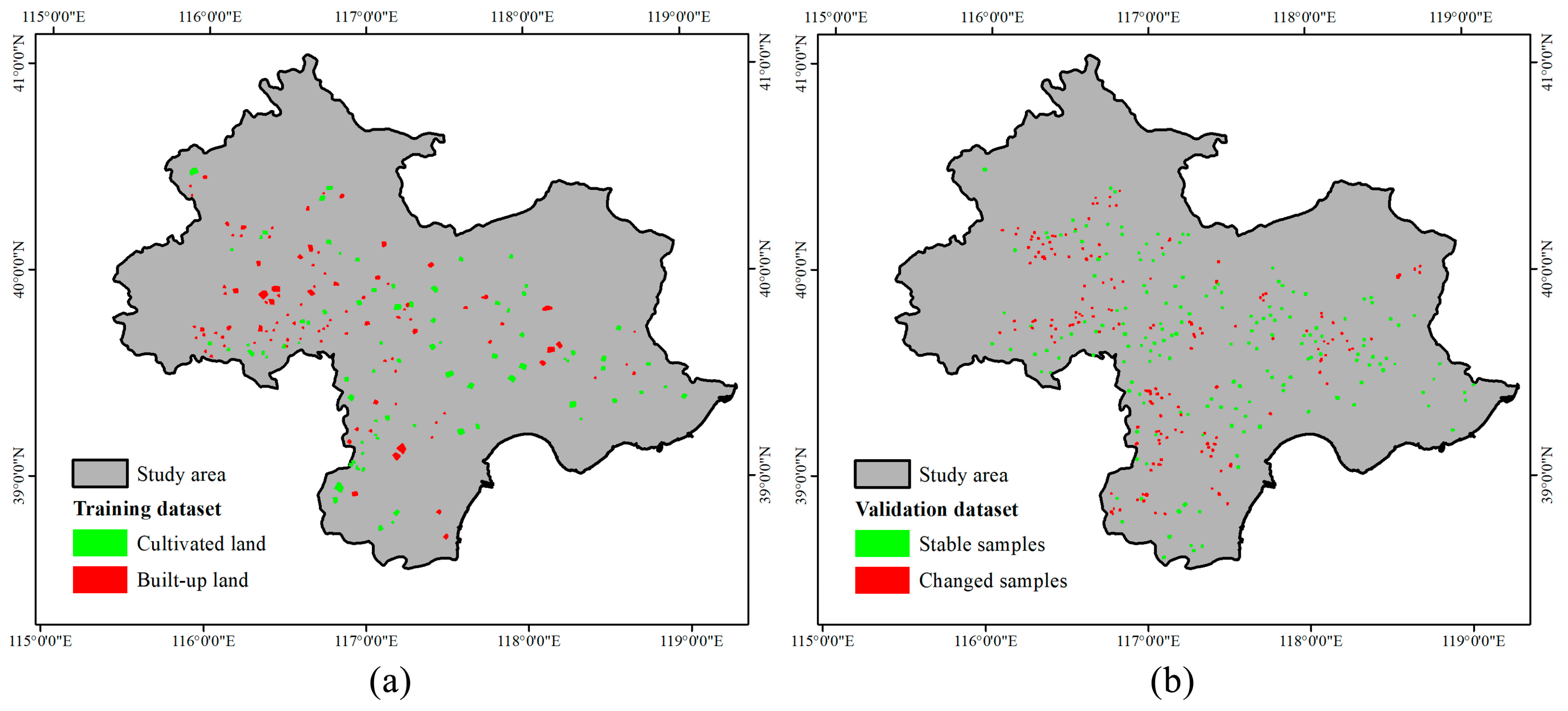
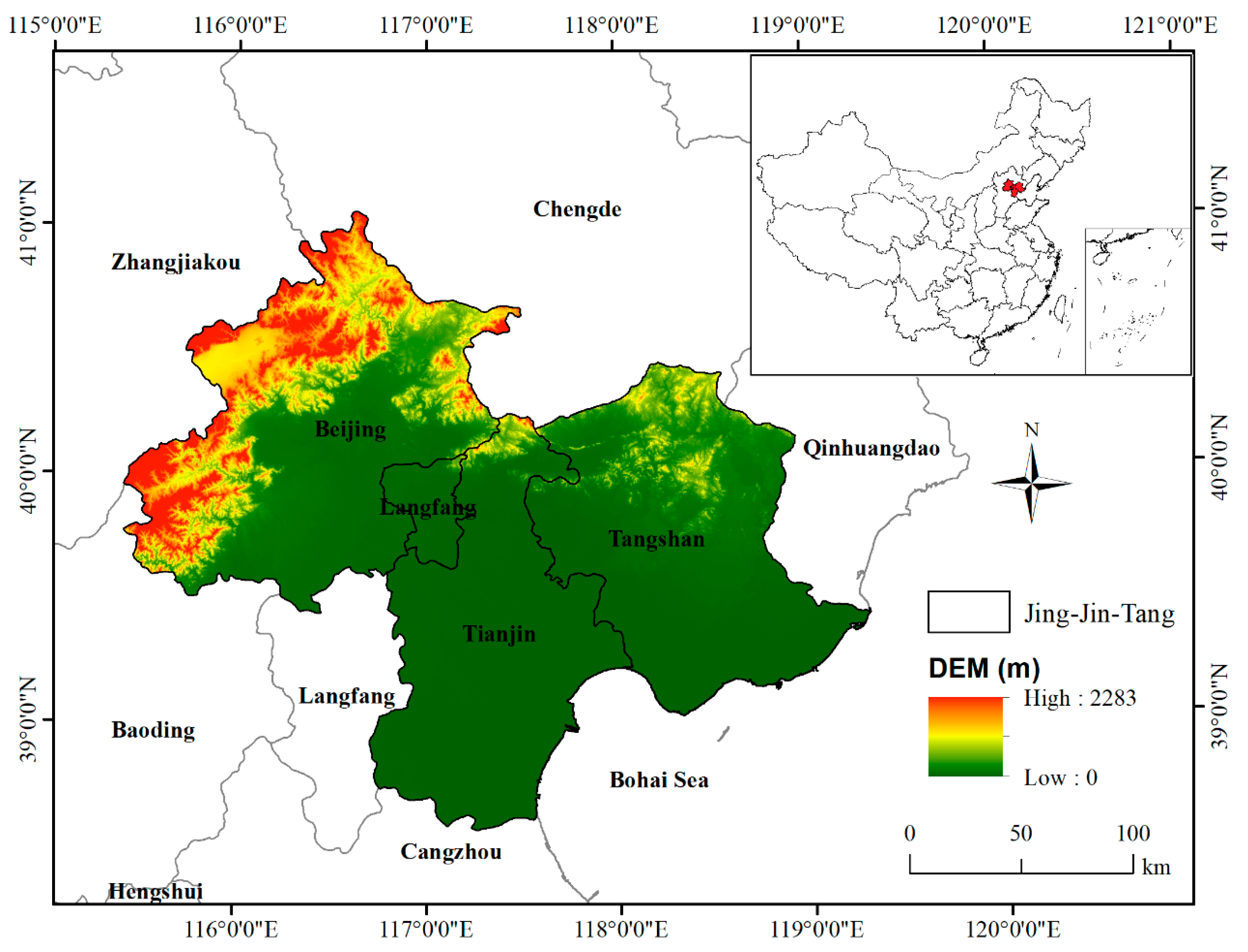
2.1. Study Area

The Beijing-Tianjin-Hebei Urban Agglomeration is located in the North China Plain, which consists of 13 cities. This region has gone through a long progress of industrialization and has become the biggest urbanized region in China [11]. Our study area consists of three main cites in the Beijing-Tianjin-Hebei Urban Agglomeration, namely, Beijing, Tianjin, and Tangshan. The enclave belonging to Langfang in Hebei province, located between Beijing and Tianjin, is also within the study area (Figure 2). The entire region is often called the Jing-Jin-Tang district, covering approximately 42,000 km² (38°30′N—41°8′N, 115°17′E—119°30′E).

Beijing, the capital city of China, plays the role of political, cultural and international communication center of the whole country. Tianjin, bordered by Beijing to the northwest, is the biggest coastal open city in northern China. Tangshan, located to the west adjoins Beijing and Tianjin, is among the most important heavy industrial cities in China. The study area is lying north of the North China Plain, located at the south side of the Yanshan Mountains, embraced by the Taihang Mountains to the west and the Bohai Sea to the east. The dominated land-cover type in this region is cultivated land, followed by forest and built-up land, as well as a small portion of water bodies, grassland, and bare land. The major crops are wheat and maize, planted mainly in the plain areas. Within the study area, large zones of cultivated land have been occupied due to urban expansion since 1979 [45]. The conversion of cultivated land to built-up land accounted for over 70% of the total farmland loss, and this proportion is even higher in the plain areas [11,46]. This makes the Jing-Jin-Tang district an ideal verification site to apply our method considering the high-speed and large-scale LULC change.

2.2. Datasets and Pre-Processing

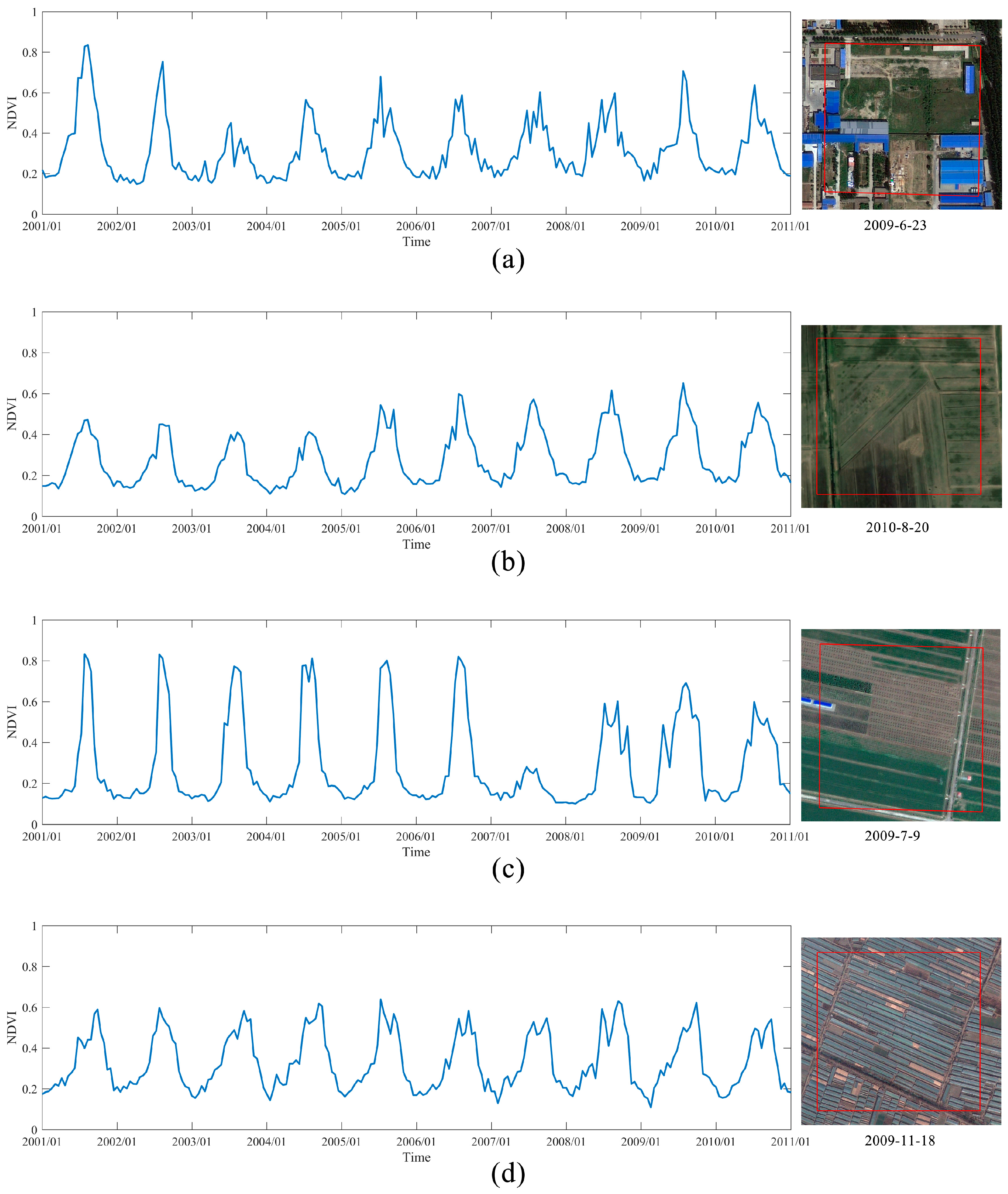
2.2.1. MODIS NDVI Time Series

The NDVI Time Series, spanning for the period from 2001 to 2011, from MODIS/Terra 16-day L3 Global 250 m products (MOD13Q1) are used in our study. The selection of these data is based on the following two observations. First, the long time-span and wide swath coverage of MODIS 250 m Vegetation Index (VI) dataset enable large-scale, long-term LULC change monitoring. Second, compared to data acquired by medium-resolution satellite sensors (such as Landsat TM/ETM+), the temporal-resolution of MODIS images is sufficiently high to composite time series at regular time intervals, which is important for retrieving comparable phenological information among different years.

Four MODIS tiles (h26v04, h26v05, h27v04, h27v05) covering the full study area were used. The tiled NDVI images were first re-projected to the UTM projection (WGS-84 Zone 50N) using the MODIS Reprojection Tool (MRT), and then mosaicked and subset over the study area for each composite period. A total of 23 images were obtained for each year and sequentially stacked into 11-year time series. Outliers caused by residual cloud and snow/ice were masked off according to the MODIS VI-quality layers. Finally, Harmonic Analysis of Time Series (HANTS) was performed on the data to deal with missing values [47]. Six harmonics was chosen to reproduce multiple agricultural growing seasons [48]. A HANTS-corrected image is shown in Figure 3. As it can be noticed, abnormal NDVI values caused by cloud contamination have been adjusted.

2.2.2. Auxiliary Data

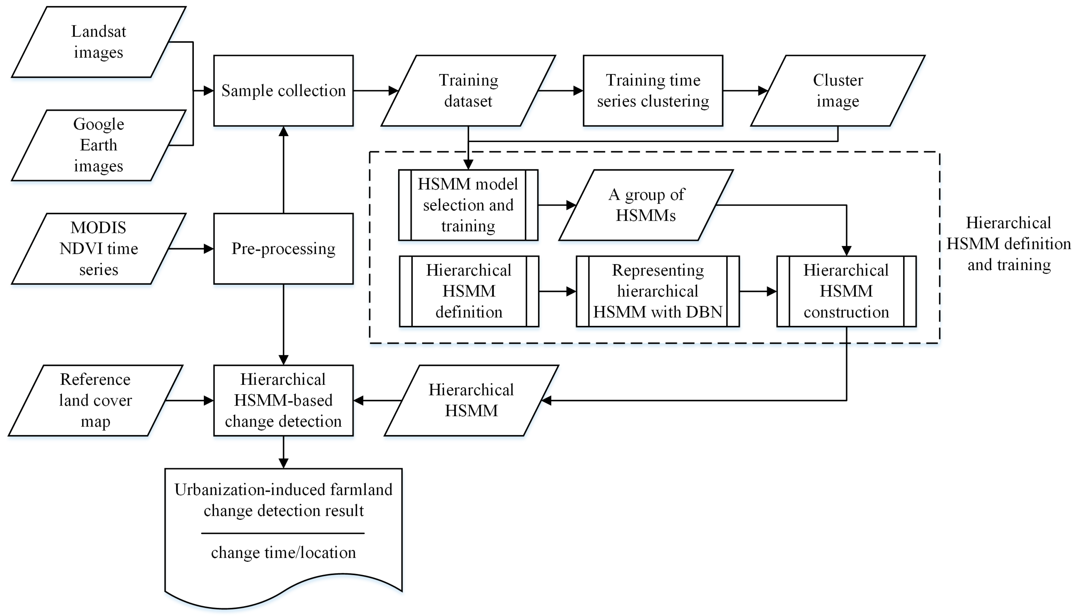
Three 100 m land-use maps of the year 2000, covering the entire study area, were used in this study as auxiliary data. They were obtained from the National Science & Technology Infrastructure of China [49]. The land-use maps were mosaicked and resampled to 250 m resolution to be consistent with the MODIS imagery, in order to create a reference map. The land-use nomenclature adopted in the reference map is the one of the National Land Use Remote Sensing Classification Scheme of Chinese Academy of Sciences, which is grouped in a two-level hierarchy, including 6 first-level classes (cultivated land, forest, grassland, water bodies, built-up land, and unused land) and 25 second-level classes [50]. In this work, we generated a mask that excluded forest, grassland, water bodies, and unused land, so as to focus our analysis on the process of urbanization-induced farmland loss. We also included built-up land in the mask to avoid confusion between cultivated land and built-up land in the beginning period due to spatial inconsistency and resampling.

A series of Landsat-5 TM images over the study area (Path123/Row32; Path122/Row32; Path122/Row33) were used for sample collection. These images were acquired during the growing seasons from 2001 to 2010, with a cloud cover less than 30%. They were used for selecting training and testing samples and determining the time of change. For example, a newly built airport occupying cultivated land was observed around 2004 in Figure 4.

3. Methodology

The proposed method includes four steps: (1) sample collection; (2) training time series clustering; (3) hierarchical HSMM definition and training; (4) hierarchical HSMM-based change detection. The overall workflow is illustrated in Figure 5.

3.1. Sample Collection

Due to the lack of ground truth data, we collected training and validation datasets through human interpretation of the Landsat images with guidance of Google Earth to lower uncertainty [51,52]. The training and testing samples are distributed evenly throughout the study area. To be consistent with a 250 m MODIS pixel size, each sample has a size of at least eight by eight pixels. All the samples are firstly digitalized on the Landsat images using the ENVI ROI tool, and then they are imported into Google Earth to confirm whether their class labels have changed from one year to another. All the samples have been validated independently by two researchers. Finally, the samples are mapped to MODIS imagery via georeferencing.

For the training samples, only regions where the land-cover types are persistent throughout the entire study period have been selected. In addition, to exclude areas with mixed land covers, we only considered samples for which the class label is unique. In total, we manually selected 2301 pixels of cultivated land and 2221 pixels of built-up land for the training set.

The validation samples were collected by visual interpretation of the first and last dates of Landsat-5 TM images. The samples belong to two categories: (a) stable pixels where farmland areas were persistent during the period of analysis; and (b) changed pixels which have converted from cultivated land to built-up land. In total, we manually selected 1463 stable pixels and 769 changed pixels in the validation set. For all the changed pixels, the years in which the changes occurred have been visually interpreted from the MODIS NDVI time series, supported by Landsat and Google Earth images.

The spatial distribution of the training and validation samples are shown in Figure 6.

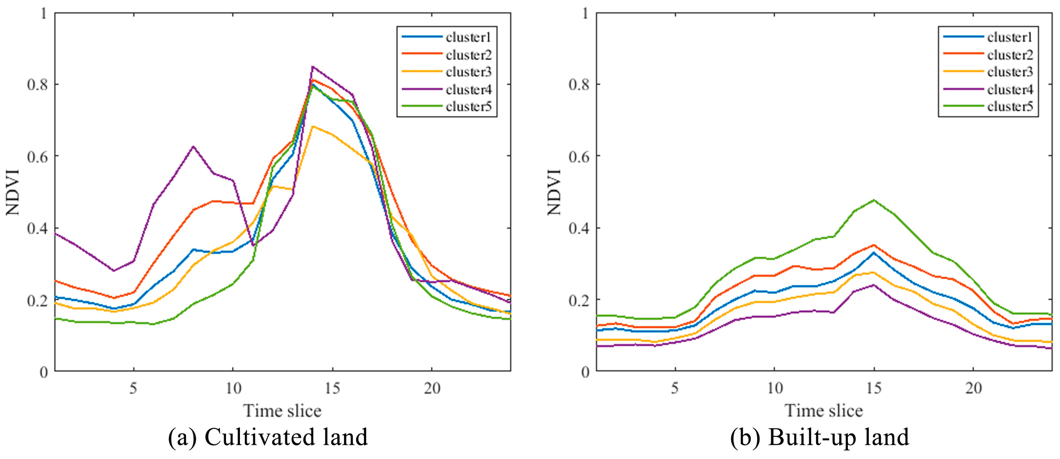
3.2. Training Time Series Clustering

As discussed in the introduction section, the spectra-temporal profiles of cultivated land are often very heterogeneous. In the case of built-up lands, they may also contain different kinds of urban plants with distinct phenological patterns. Therefore, in order to describe the complicated intra-class spectra-temporal characteristics, we use the K-Means algorithm to cluster the training samples of cultivated land and built-up land separately, thereby grouping the NDVI profiles with similar phenological patterns into clusters [30]. To deal with temporal distortions and irregular sampling, we use the dynamic time warping (DTW) measure to compare the similarity between two time-series [53]. The size of the warping window is set to 2 to limit the search of the alignment path, thereby the NDVI values of two sequences with a time delay of over a month could not be aligned together.

Here, the number of clusters K has been set to five. Figure 7 shows the averaged NDVI profiles for each land-cover type. As it can be seen, the NDVI profiles of built-up land are characterized by smooth curves with slight seasonal fluctuations (Figure 7b), whereas cultivated land is characterized by more rugged NDVI profiles with at least one narrow peak (Figure 7a), corresponding to single or double crops. The difference in the phenological pattern of cultivated land and built-up land is important for distinguish them.

3.3. Hierarchical Hidden Markov Model Definition and Training

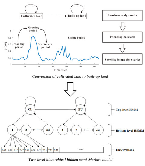
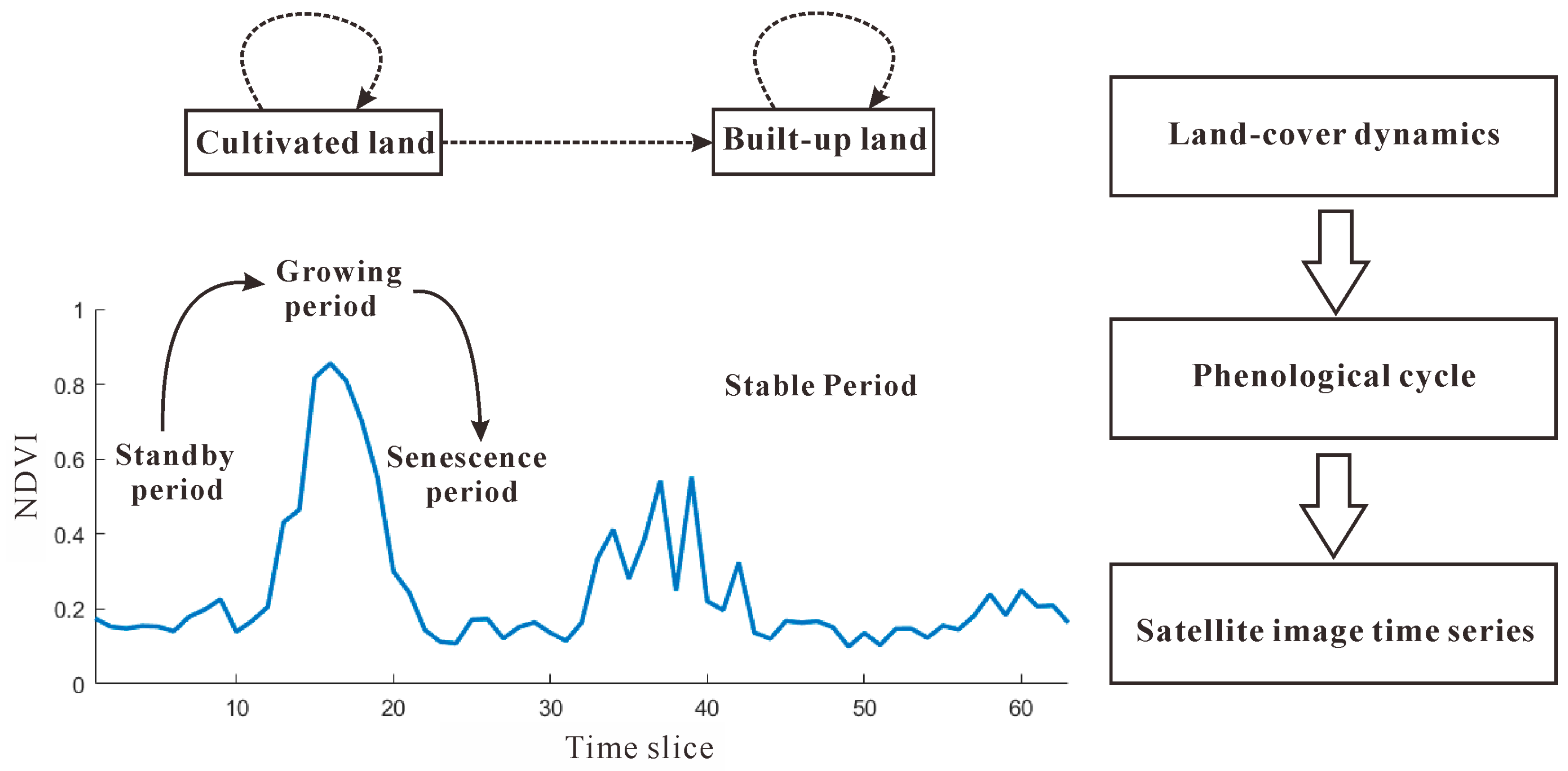
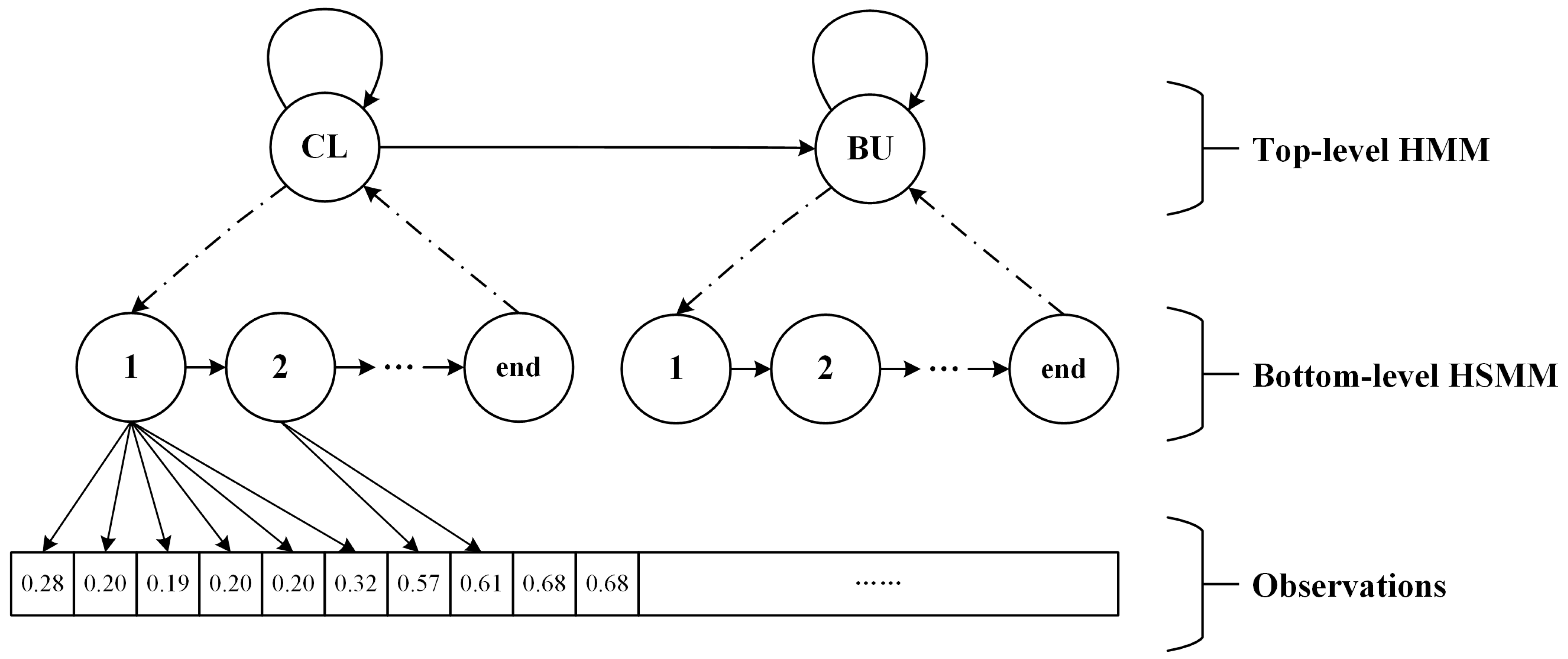
3.3.1. Hierarchical HSMM Definition

As discussed in the introduction section, hierarchical HMM extends the classical HMM and provides better modelling of sequences with hierarchical structures. A hierarchical HMM includes multiple levels of hidden states, which belong to two categories: the states at the lowest level are termed production states, and the states at higher levels are called internal states. Each internal state has its own substates. An internal state recursively activates one of its substates until a production state is reached. Only production states can emit observations. A transition between higher level states is activated only when the lower level model reaches an “end” state. The end state cannot emit observations. It only controls the termination of state transitions in the current level. Each level of a hierarchical HMM can be regarded as a “flat” HMM and is subject to Markovian hypothesis. Hierarchical HMM can correlate structures existing relatively far apart in the observation sequences, while preserving the computational tractability of simple Markov processes as well as being able to handle statistical inhomogeneity commonly occur in many complex time series data [40]. A hierarchical HMM can be represented as a dynamic Bayesian network (DBN), which speeds up the model inference and improves its practicability [54].

Since different vegetation phenological patterns within the same class will cause distinct seasonal variations in the NDVI profiles, with regards to the complexity and inherent hierarchical structure in the SITS coming from land-cover transitions and vegetation changes, the classical HMM or HSMM is limited. Therefore, in this study, we model the conversion from cultivated land to built-up land as a two-level hierarchical HMM, as illustrated in Figure 8. The model definition is given as follows.

(1) The top-level HMM

The top-level HMM represents inter-annual land-cover changes, the states in this level are internal states. In Figure 8, “CL” denotes cultivated land, and “BU” denotes built-up land. The solid lines between states in the top-level HMM denote the valid land-cover change directions, and the self-loop for each state indicates that no change happen during two consecutive years. Since a change from built-up land to cultivated land will not occur in reality, there is no transition from BU to CL. It should be noted that in the illustrated graph, CL and BU are abstract states that composed of a group of real states, respectively. Each state represents a specific phenological pattern that belongs to cultivated land or built-up land. The states belonging to the same class are fully connected (Figure 9). In this way, the intra-class variations are encoded in the proposed model.

The top-level HMM can be viewed independently as a simple Markov chain modelling the land-cover dynamics. We consider equal-probable prior distribution for all the top-level states, which is not re-estimated during the training process.

(2) The bottom-level HSMM

The bottom-level HSMM represents the annual cycle of vegetation phenology. The states in this level are implicitly related to crude phenological stages of a certain plant, and they are determined by their parent state in the top-level. The bottom-level states are production states, each of them produces a sequence of observations (NDVI values). The duration of a state indicates the length of a phenological stage, which is modelled by single Gaussian distributions. A left-right model topology with no skip path is chosen to be consistent with the annual phenological transitions.

To summarize, an observation sequence is generated by the constructed hierarchical HSMM in the following manner. First, one of the states, q, in the top-level HMM is chosen at random. Next, the first substate of q in the bottom-level HSMM is entered. A sequence of observations is emitted according to the observation probability distribution before the state transit to the next state. The bottom-level state then shifts from left to right until the end state is reached. Then the control returns to q, and the model chooses the next top-level state according to the corresponding state transition matrix. The newly chosen top-level state will start a new recursive observation generation process, and so on. Through the established model, we can infer the most probable hidden state with the highest likelihood at any time slice.

3.3.2. Dynamic Bayesian Network Representation of the Proposed Hierarchical HSMM

Following the principles of representing a hierarchical HMM as a DBN [55,56], we construct the equivalent DBN representation of the proposed two-level hierarchical HSMM, as shown in Figure 10.

In the DBN, a set of variables ${\mathsf{\Phi }}_t=\{Q_t^1,Q_t^2,F_t^2,Q_t^D,F_t^D,O_t\}$ are maintained at each time slice $t$. These variables are illustrated as nodes in the graph of Figure 10, and their cause-effect relationships are represented as edges (starting node of an edge causes the ending node). $Q_t^1$ is the current state variable in the top-level HMM. $Q_t^2$ is the current substate in the bottom-level initialized by $Q_t^1$. $F_t^2$ is a binary indicator variable that is “on” (set to 1) if the state transition terminates at time t in the bottom-level HSMM, otherwise it is “off” (set to 0). $Q_t^D$ is the state duration variable representing the residual time of current state $Q_t^2$ until time t. $F_t^D$ is a binary indicator variable that is on when $Q_t^2$ has reaches the end of its duration, otherwise it is off. Last, $O_t$ is the observed NDVI value, which is determined by both its ancestor states, i.e., $Q_t^1$ and $Q_t^2$.

The conditional probability distributions (CPDs) of nodes in the DBN can be derived from the parameters of the proposed hierarchical HSMM.

The CPD of the top-level variable $Q_t^1$ is defined as:

$$P(Q_{t+1}^1=j|Q_t^1=i,F_t^2=f)=\{\begin{array}{ll}{A}^T(i,j)& \mathrm{if}f=1\\ \delta (i,j)& \mathrm{if}f=0\end{array}$$

(1)

with $\delta (i,j)$ the Kronecker delta function which has the value 1 if $i=j$, otherwise 0. $A^T$ denotes the state transition matrix for the top-level HMM.

The CPD of the bottom-level variable $Q_t^2$ is defined as:

$$P(Q_{t+1}^2=j|Q_t^2=i,F_t^2=f_1,F_t^D=f_2,Q_{t+1}^1=k)=\{\begin{array}{ll}{\pi }_k^B(j)& \mathrm{if}{f}_1=1,\mathrm{and}{f}_2=1\\ {\tilde{A}}_k^B(i,j)& \mathrm{if}{f}_1=0,\mathrm{and}{f}_2=1\\ \delta (i,j)& \mathrm{if}{f}_2=0\end{array}$$

(2)

where ${\pi }_k^B$ is the initial state distribution of the bottom-level HSMM given that the parent variable is in state $k$, and ${\tilde{A}}_k^B$ is the rescaled version of the state transition matrix, excluding the end state. When $F_t^D=0$, the bottom-level variable $Q_{t+1}^2$ remains in the same state to the next time slice. When $F_t^D=1$, there are two possibilities: if $F_t^2=1$, the top-level variable $Q_{t+1}^1$ will convert to state $k$ at time t + 1 and initialize a new semi-Markov chain according to the initial state distribution; if $F_t^2=0$, $Q_{t+1}^1$ will remain in the same state at time t + 1 while $Q_{t+1}^2$ will shift to a new substate.

Since a left-right model topology is assumed for all the bottom-level HSMMs, $F_t^2=1$ only if the rightmost state reaches the end of its duration. Hence, the CPD $F_t^2$ is written as:

$$\begin{array}{l}P(F_t^2=1|Q_t^2=i,F_t^D=f)=\{\begin{array}{ll}\delta (i,N)& \mathrm{if}f=1\\ 0& \mathrm{if}f=0\end{array}\\ P(F_t^2=0|Q_t^2=i,F_t^D=f)=1-P(F_t^2=1|Q_t^2=i,F_t^D=f)\end{array}$$

(3)

where $N$ is the number of states in the bottom-level HSMM.

The CPDs of the state duration variable $Q_t^D$ and the indicator variable $F_t^D$ are defined as:

$$P(Q_{t+1}^D=d^{\prime }|Q_t^D=d,F_t^D=f,Q_{t+1}^2=i,Q_{t+1}^1=k)=\{\begin{array}{ll}{D}_{k,i}(d^{\prime })& \mathrm{if}f=1\\ \delta (d^{\prime },d-1)& \mathrm{if}f=0\end{array}$$

(4)

$$\begin{array}{l}P(F_t^D=1|Q_t^D=d)=\delta (d,0)\\ P(F_t^D=0|Q_t^D=d)=1-P(F_t^D=1|Q_t^D=d)\end{array}$$

(5)

where $D_{k,i}$ is the state duration distribution given that $Q_{t+1}^1$ is in state $k$ and $Q_{t+1}^2$ is in state $i$. When $F_t^D=0$, $Q_t^D$ decreases by one each time. When $F_t^D=1$, $Q_{t+1}^2$ will convert to the next state at time t + 1, and a new sample is drawn from the state duration distribution. When $Q_t^D$ decreases to zero, then $F_t^D=1$, otherwise $F_t^D=0$.

Finally, the CPD of observation $O_t$ is defined as:

$$P(O_t=y|Q_t^2=i,Q_t^1=k)=\mathcal{N}(y;{\mu }_{k,i},{\sigma }_{k,i}^2)$$

(6)

where $\mathcal{N}({\mu }_{k,i},{\sigma }_{k,i})$ is a Gaussian function with mean ${\mu }_{k,i}$ and variance ${\sigma }_{k,i}^2$, given that $Q_{t+1}^1$ is in state $k$ and $Q_{t+1}^2$ is in state $i$.

3.3.3. Hierarchical HSMM Construction

We construct the proposed hierarchical HSMM in a “bottom-up” manner. First, we derive the parameters of the bottom-level model from a group of pre-trained HSMMs. Second, the state transition matrix in the top-level HMM, which corresponds to the land-cover transition probabilities, is learned using unlabeled time series.

1. HSMM Model Selection and Training

To avoid the pseudo changes caused by the intra-class variations, we should train an individual HSMM for each phenological pattern. Based on the time series clustering results, we train an HSMM for each cluster individually, making use of the training samples. The entire 11-year NDVI time series are used for model fitting to avoid phase shifts among different years. We utilize the Akaike Information Criterion (AIC) to determine the optimal model structure, i.e., the number of hidden states in an HSMM. The AIC value is defined by the maximum likelihood of the model, coupled with a penalty term which takes into account of the model complexity [57]:

$$AIC=\frac{-\log L(\widehat{\theta })+p}{T}$$

(7)

where $L(\widehat{\theta })$ denotes the likelihood of the model with parameter $\widehat{\theta }$; $p$ is the number of model parameters. The best model that minimizing Equation (7) is chosen.

Once a group of well-trained HSMMs are learned, the parameters of the proposed model in the bottom-level are obtained referring to Equations (1)–(6).

2. Land-Cover Change Probabilities Estimation

We randomly selected 3000 unlabeled, evenly distributed pixels to estimate the land-cover transition probabilities, according to the reference map. Their 11-year time series are fed to the DBN to optimize the state transition matrix in the top-level HMM, which has been randomly initialized. As some of those pixels have experienced a farmland-to-urban change during 2001–2011, the change probability of the study area over the period of analysis is estimated from the data. It should be noted that since the change probability from built-up land to cultivated land is initialized to zero, it is not updated during the model training procedure.

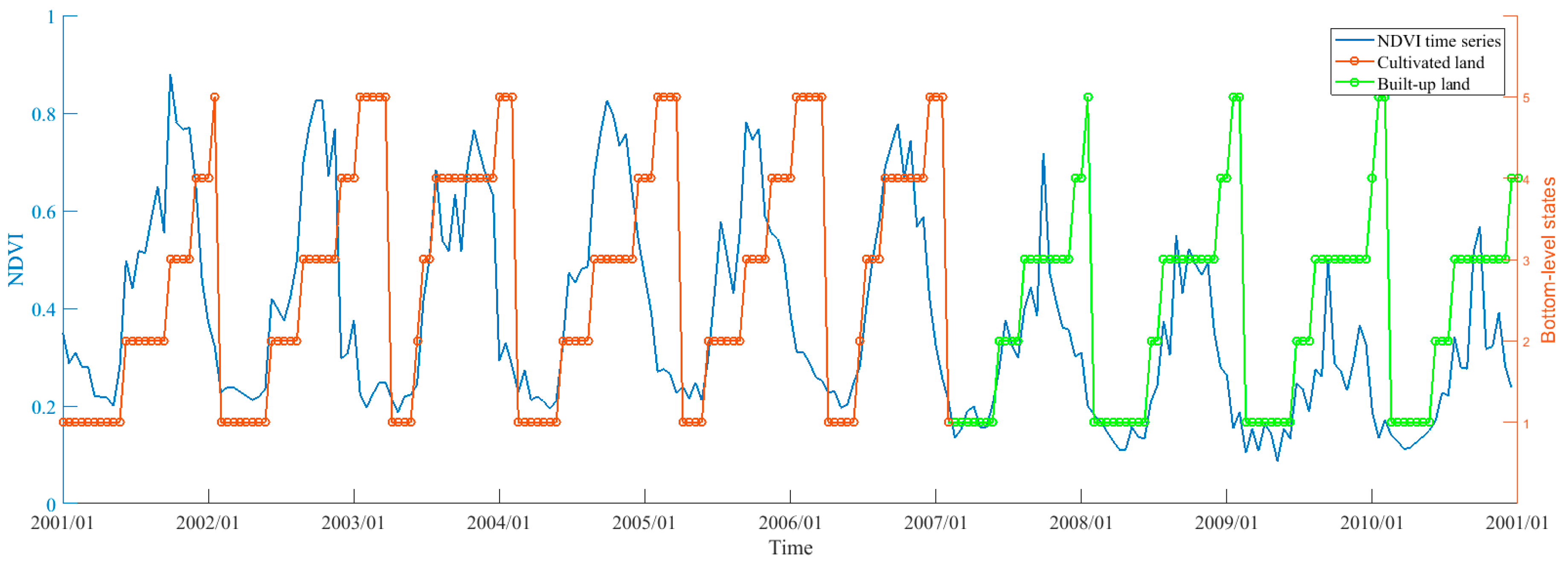
3.4. Hierarchical HSMM-based Change Detection

Once the proposed hierarchical HSMM is learned, we can use the model to identify farmland-to-urban changes from long-term SITS. Given the time series of a pixel, the most probable sequence of states is estimated by the junction tree (jtree) algorithm [54]. Hence, we can obtain the land-cover change history of the pixel over the entire study period. The time slice when the top-level state converts from CL to BU is the detected change time. Since the intra-class variations is not viewed as a real land-cover change, our algorithm is robust to inter-annual changes across different crop species and cultivation practices.

For example, Figure 11 illustrates an NDVI time series and the estimated state sequence. 5-states is chosen in the bottom level HSMM. We use different colors to differentiate CL and BU in the top-level HMM: red represents CL while green represents BU. It can be seen clearly that our method not only can estimate the phenological transitions, but also correctly identify the land-cover change round 2007.

4. Results

In this section, we first illustrate the results of model selection, and then we apply the method to real-world dataset for mapping newly built areas encroached onto farmland in the Jing-Jin-Tang district.

4.1. Model Selection for HSMM

The goal of this experiment was to select the best number of states in the bottom-level HSMM to simulate the seasonal variations of intra-annual NDVI time series. For this purpose, a series of model learning procedure were carried out on the training data, each one with a variable number of states, N, ranging from 2 to 8. Since accurate parameter initialization is essential for satisfying model fitting, we fitted an HSMM 50 times with random initialization to obtain the optimal model parameters for each cluster. For each model structure, the AIC value defined in Equation (7) was evaluated.

The obtained results are shown in Figure 12. It can be noticed that for both classes, the best value of N ranges from 4 to 7. For most clusters, the AIC values do not improve much by using more than 5 states. It means that the performance improvement brought to the model by adding more states is trivial. Therefore, 5 has been considered as the optimal number of states for the bottom-level HSMM.

4.2. Change Detection Accuracy and Method Comparisons

In this experiment, we mapped cultivated land and built-up land by the proposed algorithm from 2001 to 2010 for the entire study area. To verify the effect of incorporating the land-cover conversion information, we compared our method with the post-classification algorithm based on HSMM: for each pixel, the intra-annual NDVI time series in 2001 and 2010 were classified individually and then compared to detect changes. We also compared our method with two other algorithms that were previously used for time series change detection, i.e., random forests (RF) [58] and CCDC [28]. The RF classifier was made of 5000 single trees and trained with all the NDVI observations in each year (23-dimensional features). The RF classifications resulted in 11 annual maps spanning from 2001 to 2011. We also assessed the results of RF with a 3-year temporal filtering [25], denoted as RF-TF in the following. For CCDC, the threshold used for change detection was set to the RMSE. When a change was identified, the online change detection process in CCDC is terminated and the change time is recorded.

For all the methods, confusion matrices were generated to calculate the user’s and producer’s accuracy, the overall accuracy, and the Kappa coefficients. In addition, the temporal accuracy was assessed for all the changed pixels that were correctly detected. Here, the term “temporal accuracy” is defined as the proportion of pixels that have the same change year between the detection results and the reference data [28].

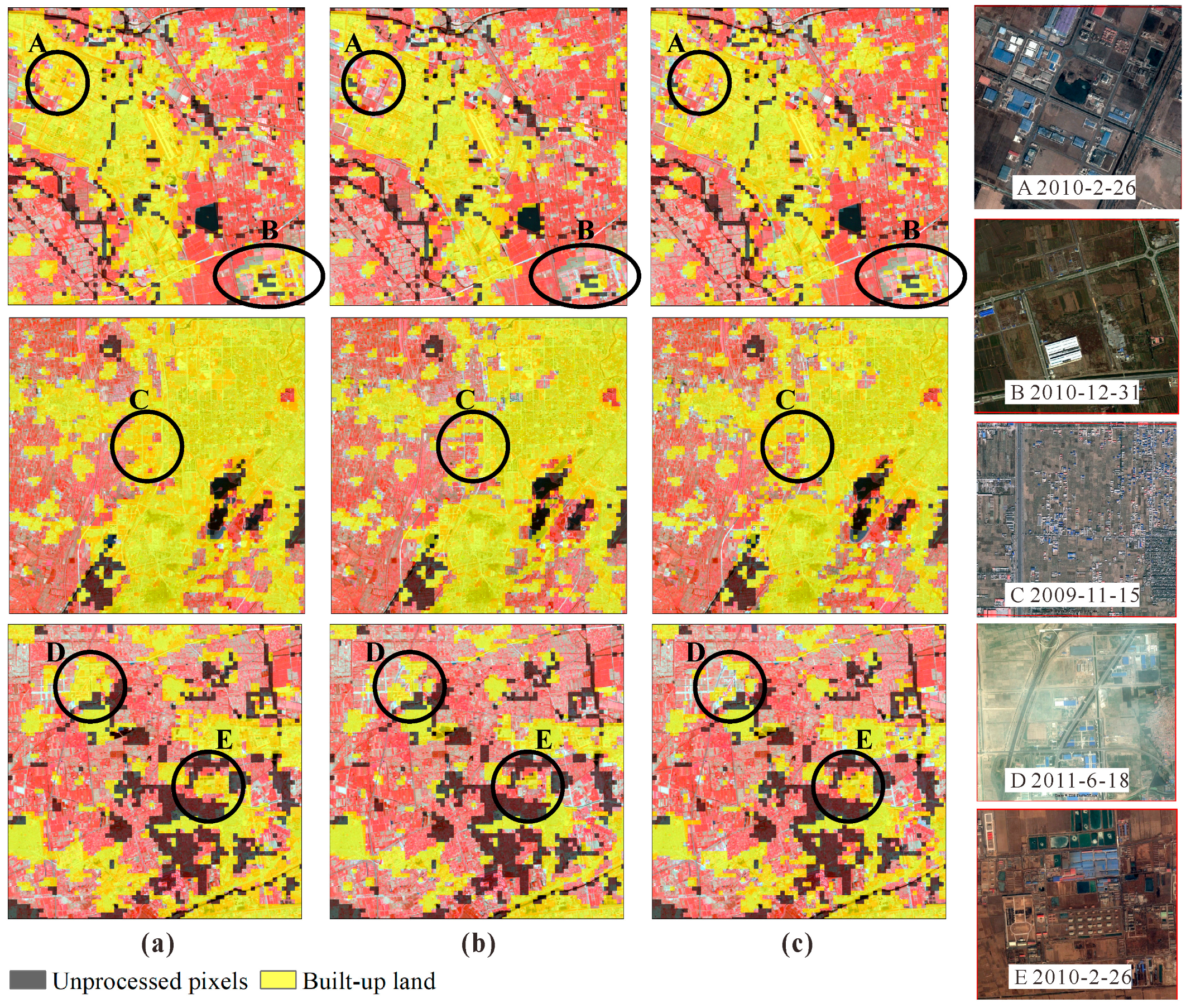
4.2.1 Accuracy Assessment for Change Location

The land-cover maps for 2001 and 2010 obtained by the proposed algorithm are shown in Figure 13. By visual comparison, we found that the classification results were very close to the ground truth. In order to compare the differences between different methods, three subset images are illustrated in Figure 14. As it can be seen, the proposed method performs relatively better in identifying partially changed pixels. In particular, the proposed method is more sensitive to linear man-made structures such as roads (areas of B and D), exposed construction sites (areas of A and E), as well as urban areas with mixed covers (area of C).

The performance of these methods was evaluated on the validation set, and the results are listed in

Table 1. Change detection assessment of the proposed method.

Prediction	Reference
	Stable Pixels	Changed Pixels	Total	User’s Accuracy (%)
Stable pixels	1437	25	1462	98.29
Changed pixels	26	744	770	96.62
Total	1463	769	2232	-
Producer’s Accuracy (%)	98.22	96.75	-	-
Overall Accuracy = 97.72% Kappa coefficient = 0.950

,

Table 2. Change detection assessment of HSMM-based post-classification algorithm.

Prediction	Reference
	Stable Pixels	Changed Pixels	Total	User’s Accuracy (%)
Stable pixels	1422	111	1533	92.76
Changed pixels	41	658	699	94.13
Total	1463	769	2232	-
Producer’s Accuracy (%)	97.20	85.57	-	-
Overall Accuracy = 93.19% Kappa coefficient = 0.846

,

Table 3. Change detection assessment of the RF algorithm.

Prediction	Reference
	Stable Pixels	Changed Pixels	Total	User’s Accuracy (%)
Stable pixels	1443	64	1507	95.75
Changed pixels	20	705	725	97.24
Total	1463	769	2232	-
Producer’s Accuracy (%)	98.63	91.68	-	-
Overall Accuracy = 96.24% Kappa coefficient = 0.916

,

Table 4. Change detection assessment of the RF-TF algorithm.

Prediction	Reference
	Stable Pixels	Changed Pixels	Total	User’s Accuracy (%)
Stable pixels	1446	49	1495	96.72
Changed pixels	17	720	737	97.69
Total	1463	769	2232	-
Producer’s Accuracy (%)	98.84	93.63	-	-
Overall Accuracy = 97.04% Kappa coefficient = 0.933

and

Table 5. Change detection assessment of the CCDC algorithm.

Prediction	Reference
	Stable Pixels	Changed Pixels	Total	User’s Accuracy (%)
Stable pixels	1409	103	1512	93.19
Changed pixels	54	666	720	92.50
Total	1463	769	2232	-
Producer’s Accuracy (%)	96.31	86.61	-	-
Overall Accuracy = 92.97% Kappa coefficient = 0.842

. It is clear the proposed algorithm has achieved the highest precision with overall accuracy of 97.72% and Kappa coefficient of 0.950. Compared to the HSMM-based post-classification algorithm (with the overall accuracy of 93.19% and Kappa coefficient of 0.846), it can be seen that due to the use of land-cover transition knowledge, all the accuracy metrics have been improved greatly. Both commission and omission errors for changed pixels deceased, resulting in the producer’s accuracy raising from 85.57% to 96.75%, and the user’s accuracy increasing from 94.13% to 96.62%. The results from RF-TF are also better than RF, with the overall accuracy of 97.04%, and Kappa coefficient of 0.933, which are comparable with the proposed algorithm. It demonstrates that post-classification algorithm based on RF-TF is also effective in differentiating farmland-to-urban changes from no-change with all the intra-annual NDVI observations. However, though temporal filtering can somewhat improve the accuracy, the omission errors in RF-TF are still relatively high, for some farmland pixels are misclassified to built-up land from the very beginning (mainly due to cropland abandonment). The misclassifications in the initial phase cannot be corrected even though some abandoned croplands were re-cultivated latter. CCDC performs the worst in comparison to the other algorithms, with the lowest overall accuracy of 92.97%, and Kappa coefficient of 0.842. This is because the simple harmonic model adopted by CCDC is incompatible with the complex phenological dynamics of cultivated land with more than one growing season [19].

The omission errors of the proposed algorithm are mainly due to the mixture of different land covers within the same pixel. In Figure 15a, a large part of the area is covered with grasses and shrubs, so the magnitude of the NDVI decrease is relatively small. With respect to the commission errors, they mostly result from the following reasons: 1) abandoned or unused farmland (farmland areas that have not been cropped for more than two years); 2) a sharp drop in the peak of the NDVI profile; 3) the coverage of greenhouse. First, the NDVI profiles of abandoned or unused farmland are easily confused with construction sites. For example, in Figure 15b, the farmland fields have been abandoned during the entire study period, resulting in the corresponding pixel misclassified as built-up land in all scenes. The reason is that it is hard to distinguish between bare land and built-up land due to their similar spectral signatures and the coarse spatial resolution of MODIS, as previous research has confirmed [59,60]. Second, the intra-annual NDVI time series completely inconsistent with the seasonal variations of cultivated land could also lead to false change alarms. In Figure 15c, the NDVI time series of the pixel drop dramatically in 2007, leading the model to infer a land-cover change. This phenomenon may be caused by farmland fallowing, meteorological disasters, crop diseases and insect pests, etc. Third, the spectral and temporal characteristics are quite similar between plastic greenhouses and man-made infrastructures [61]. It is almost impossible to distinguish farmland covered by greenhouses from built-up land only from the NDVI time series (Figure 15d).

4.2.2. Accuracy Assessment for Change Year

The temporal accuracy was assessed through the proposed algorithm, RF-TF, and CCDC. The results are given in

Table 6. The accuracy assessment of change detection in the temporal domain.

Prediction	Reference		Temporal Accuracy (%)	Temporal Accuracy ± 1 yr (%)
	Correct	Total
The proposed method	555	744	74.60	86.29
RF-TF	508	720	70.56	85.83
CCDC	324	666	48.65	74.77

. Among the 744 changed pixels that have been detected by the proposed algorithm, the change times of 555 pixels are the same as the visual interpretation results, and the temporal accuracy is as high as 74.60%, greater than 70.56% of RF-TF and 48.65% of CCDC. It demonstrates that the detection accuracy of the proposed method is much better than its competitors in the temporal domain.

The temporal errors of the proposed algorithm are mostly due to the fact that urban construction projects within a 250 m by 250 m MODIS pixel could take more than one year to complete. The initial change time of a partially changed pixel is difficult to identify, since the magnitude of change in the NDVI time series is slight. However, most of the changes may be detected later when it is totally changed. In addition, during the process of cultivated land turning into built-up land, the fields usually first become bared or covered with weeds, which may lead to inaccurate detection. If we relaxed the precision to ±1 year, the temporal accuracy increased significantly for all the algorithms (Table 6). The proposed algorithm is still the best performer at 86.29% accuracy, while RF-TF is at 85.83% and CCDC is at 74.77%.

5. Discussion

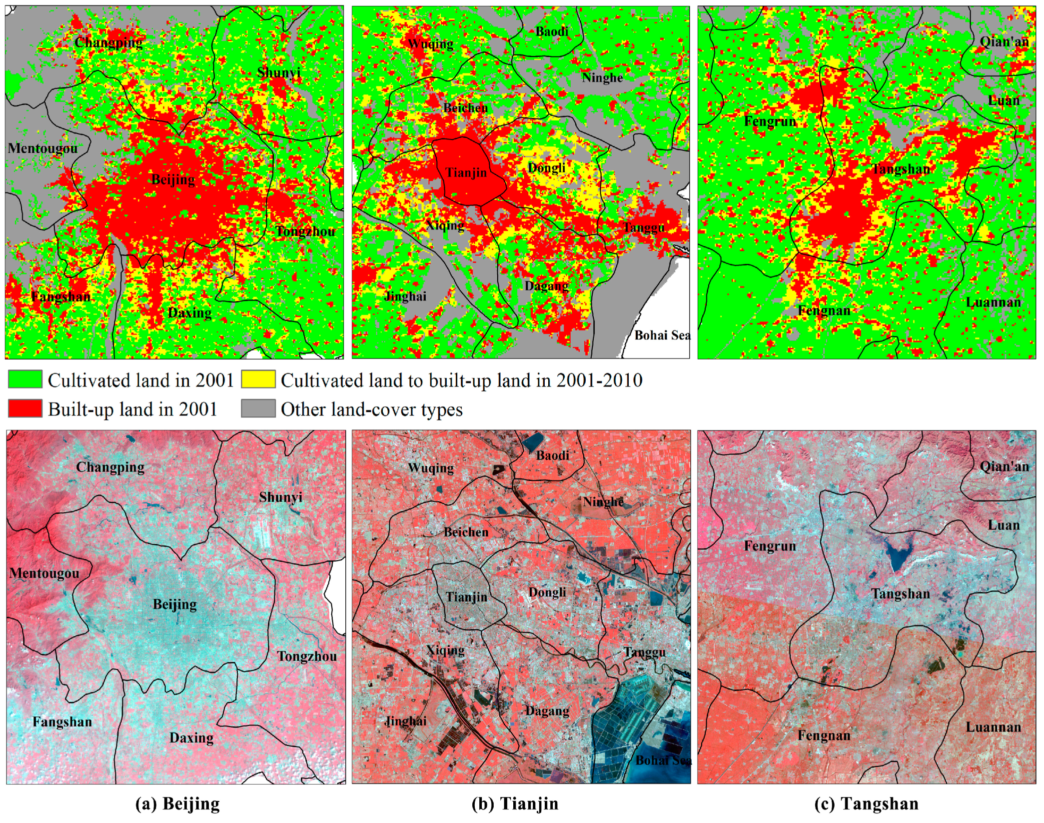
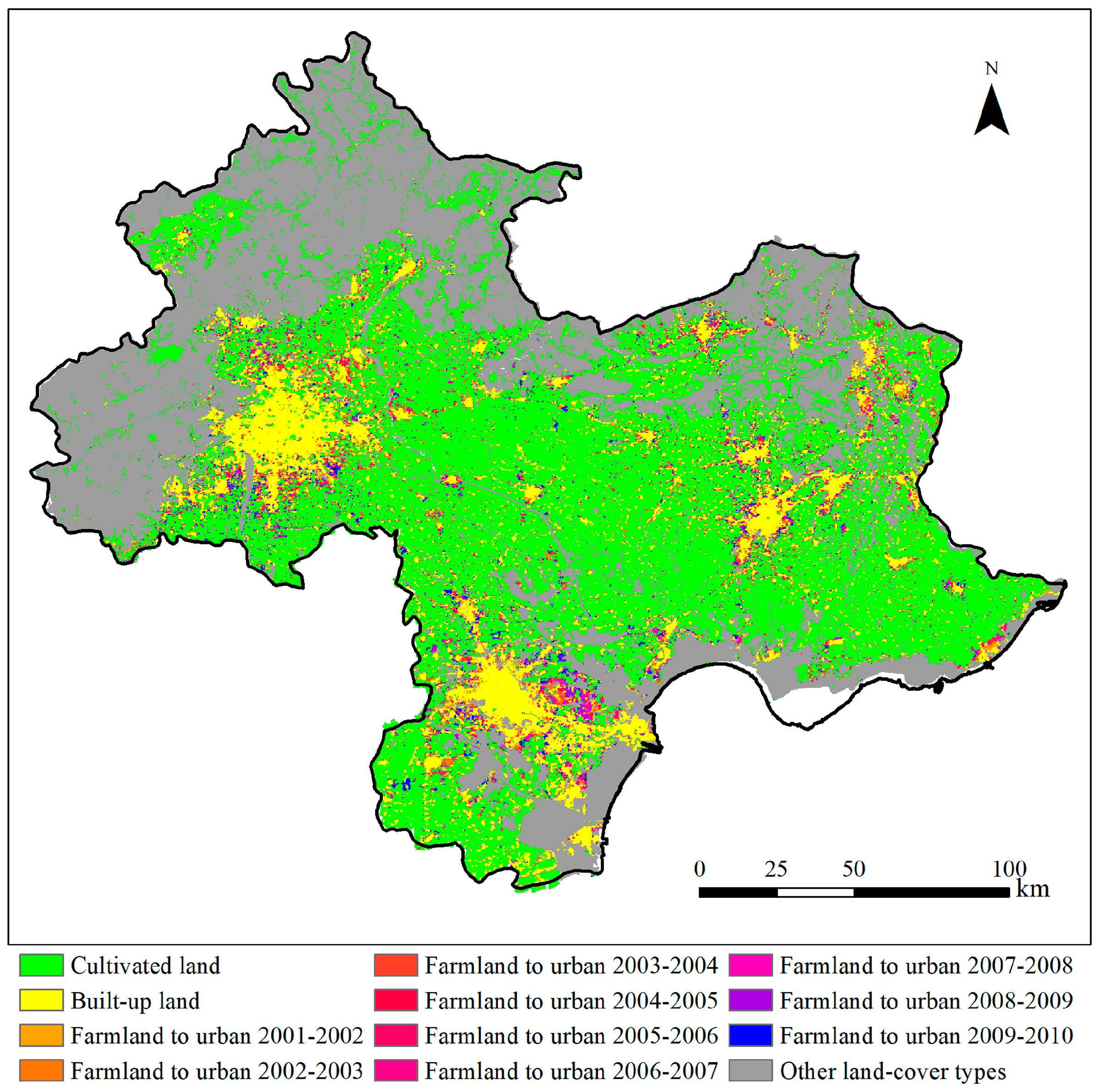
5.1. Urban Expansion Patterns in the Jing-Jin-Tang District

Based on the above results, the annual land-cover change detection results produced by the proposed algorithm are shown in Figure 16. Between 2001 and 2010, the total area of urbanization-induced farmland loss was reached by 2514 km², accounting for 11.9% of the total cultivated land areas in 2001. The largest amount of farmland loss occurred during 2001–2004 and 2008–2010.

For Beijing, 16.3% of the cultivated land areas have changed to built-up areas. According to Figure 17a, the new built-up areas were developed almost in every direction, radiating outward from the existing urban centers. In comparison, cultivated lands distributed in the outer suburbs have changed little. It demonstrates that Beijing has reflected a typical mononuclear polygon urbanization pattern, as reported in [62]. In 2001–2010, the city’s 5th and 6th Ring Roads were built around the urban core, which has greatly improved the traffic efficiency of Beijing. This led to the economic development along the roads and rapid urbanization progress. Due to this effect, most of the newly urbanized regions were concentrated between the 4th and 6th Ring Roads, as mentioned in [63].

For Tianjin, 11.2% of the cultivated land areas has changed to built-up areas. According to Figure 17b, the newly built areas were extended eastward from the main urban district towards the coastline. The area is concentrated in the Dongli district, along the Beijing-Tianjin-Tanggu Expressway. These results are consistent with the ones obtained in [62] that with the simultaneous urban growth in the main city and the Binhai New Area, the latter in the southeast coast is gradually combined with the former into a line from 2000 to 2010. Moreover, according to the Urban Master Plan of Tianjin (2005-2020), the axis along the Haihe River and the Beijing-Tianjin-Tanggu Expressway is taken as the main shaft of urban development [63], therefore, the observed phenomenon is likely to continue in the future.

For Tangshan, 9.9% of the cultivated land areas have converted to built-up areas. According to Figure 17c, the urban expansion in Tangshan toke both around the city’s urban core and in the suburbs, reflecting a compact, multiple-nuclei urbanization pattern. Some hotspots were clearly delineated, including: (a) the Phoenix New Town, the Tangshan Fengnan Economic Development Zone, and the Kaiping High-tech Zone around the main urban district; (b) the transportation hub in the Fengrun district. From this phenomenon, we can draw the following conclusions: with the urban-rural population growth, increasing residential land assumption has been one of the major reasons for urban expansion in Tangshan. In addition, demand for industrial land was another driving force accompanied by the construction of new industrial parks. Finally, it is found that the transport infrastructure played a role in the distribution of newly urbanized areas.

In summary, the results show that the spatial characteristics of urban expansion in the Beijing-Tianjin-Tangshan district is closely linked to the urban planning policy and the traffic infrastructure.

5.2. Strengths and Limitations of the Proposed Algorithm

The proposed algorithm has been designed for long-term urbanization-induced farmland loss monitoring based on SITS. In comparison with other state-of-the-art algorithms, this method has some remarkable advantages. First, no threshold is needed for the change detection process. In CCDC, the change threshold is a critical parameter and should be carefully selected. If it is set smaller, the omission errors are reduced at the expense of more commission errors, or vice versa. The proposed method saves the effort of threshold filtering and suppresses the omission errors and commission errors as well. Second, the proposed model takes into consideration of the intra-class variations in cultivated land. The proposed hierarchical HSMM encodes the complex phenological patterns in cultivated land induced by various crop types or cultivation practices, which makes it robust to pseudo changes. Third, the proposed method makes full use of the temporal information of the entire time series to infer the land-cover type of a pixel at each time slice. In comparison, both post-classification (i.e., RF-TF and HSMM) and profile-based algorithms (i.e., CCDC) identify the class label of a pixel using only a few observations before or after the current time. This explains why the proposed algorithm can improve the temporal accuracy.

Despite the above-mentioned strengths, there still exist some limitations. The primary limitation of the proposed algorithm is that we consider only cultivated land and built-up land, while other classes are ignored in the established hierarchical HSMM to simplify the model structure. Hence, the proposed method is more applicable to areas where farmland-to-urban is the dominant type of land-cover dynamics, which is the case in many fast-urbanized regions in developing countries. However, other land-cover changes (especially from cultivated land to bare land) may affect the results of the analysis. Fortunately, this is not an inherent limitation of the hierarchical HSMM itself. This problem could be solved by incorporating all related land-cover types into the model.

6. Conclusions

Better knowledge of the extent and spatial patterns of urbanization-induced farmland loss is important to assess the environmental outcomes of the urban expansion process and to predict future urban development. We developed a methodology to identify urban encroachment onto farmland areas using MODIS NDVI time series. Specifically, the farmland-to-urban change process is modelled by a two-level hierarchical HSMM: the bottom layer represents vegetation phenological stages and their durations using HSMMs; the top layer represents the land-cover conversions where each state is made of a sequence of phenological stages. Land-cover changes are detected by inferring whether the states in the top layer has changed. This hierarchical architecture enables us to encode the multi-level semantic information of SITS at different time scales. Specifically, intra-annual series reflect phenological differences and inter-annual series reflect land-cover dynamics. In this way, we can make use of these information to determine the change locations and times. As case study, we applied the proposed method to detect transitions from cultivated land to built-up land in the Jing-Jin-Tang district, China from 2001 to 2010. The performance of the proposed method is evaluated and compared with other algorithms. The experimental results demonstrate that the proposed method is superior in detection accuracy in both spatial and temporal domains. In addition, the spatial-temporal patterns of urban expansion revealed in this study are consistent with the findings of previous studies, which also confirms the effectiveness of the proposed method. The long-term urban expansion mapping results achieved by the proposed method can serve as a baseline for socio-economic analysis as well as for studies of landscape dynamics and urban planning.

There are still many aspects that we can improve in the current work. (1) The influence of mixed pixels can be greatly reduced by using data with a higher spatial resolution, such as images from sensors like Sentinal-2. The accumulation of imagery by these newly launched satellites will provide purer observations and will improve the performance of the proposed method. (2) The proposed method does not directly link the plant phenology to the model. Though some studies have proposed to learn species-specific HMMs for crop classification and phenology monitoring [32,33], they are not compatible with coarse resolution remote sensing observations. In the MODIS imagery, each pixel reflects the integrated response across various species [64]. In this regard, we propose to use K-Means to group the NDVI profiles of each class into clusters with homogeneous phenological behaviors. Since incorporating knowledge of plant phenology into the model will offer potential for more accurate cultivated land discrimination, as well as making the model inference results easier to understand, this may be a promising avenue for further research on high-resolution SITS. (3) In addition to urban expansion monitoring, the proposed method is also applicable for many other environmental issues, such as monitoring abandoned cultivated land, soil erosion and desertification, deforestation, and changes in continental coastline, etc. These studies may be conducted in our future works to broaden the application scope of the proposed method.

References

1. Lopez, T.D.; Aide, T.M.; Thomlinson, J.R. Urban Expansion and the Loss of Prime Agricultural Lands in Puerto Rico. Ambio 2001, 30, 49–54. [Google Scholar] [CrossRef] [PubMed]
2. Thapa, R.B.; Murayama, Y. Examining spatiotemporal urbanization patterns in Kathmandu Valley, Nepal: Remote sensing and spatial metrics approaches. Remote Sens. 2009, 1, 534–556. [Google Scholar] [CrossRef]
3. Pandey, B.; Seto, K.C. Urbanization and agricultural land loss in India: Comparing satellite estimates with census data. J. Environ. Manag. 2015, 148, 53–66. [Google Scholar] [CrossRef] [PubMed]
4. Pribadi, D.O.; Pauleit, S. The dynamics of peri-urban agriculture during rapid urbanization of Jabodetabek Metropolitan Area. Land Use Policy 2017, 48, 13–24. [Google Scholar] [CrossRef]
5. Bai, X.; Shi, P.; Liu, Y. Society: Realizing China’s urban dream. Nature 2014, 509, 158–160. [Google Scholar] [CrossRef] [PubMed]
6. Shi, K.; Chen, Y.; Yu, B.; Xu, T.; Li, L.Y.; Huang, C.; Liu, R.; Chen, Z.; Wu, J. Urban expansion and agricultural land loss in China: A multiscale perspective. Sustainability 2016, 8, 790. [Google Scholar] [CrossRef]
7. China Statistical Yearbook 2017. National Bureau of Statistics of the People’s Republic of China, 2017. Available online: http://www.stats.gov.cn/tjsj/ndsj/2017/indexch.htm (accessed on 30 September 2018).
8. Zhang, Z.; Wen, Q.; Liu, F.; Zhao, X.; Liu, B.; Xu, J.; Yi, L.; Hu, S.; Wang, X.; Zuo, L.; et al. Urban expansion in China and its effect on cultivated land before and after initiating “Reform and Open Policy”. Sci. China Earth Sci. 2016, 59, 1930–1945. [Google Scholar] [CrossRef]
9. Tan, M.; Li, X.; Lu, C. Urban land expansion and arable land loss of the major cities in China in the 1990s. Sci China Ser D 2005, 48, 1492–1500. [Google Scholar] [CrossRef]
10. Chen, L.; Jiang, P.; Chen, W.; Li, M.; Wang, L.; Pian, Y.; Xia, N.; Duan, Y.; Huang, Q. Farmland protection policies and rapid urbanization in China: A case study for Changzhou City. Land Use Policy 2015, 48, 552–566. [Google Scholar] [CrossRef]
11. Tan, M.; Li, X.; Xie, H.; Lu, C. Urban land expansion and arable land loss in China—a case study of Beijing–Tianjin–Hebei region. Land Use Policy 2005, 22, 187–196. [Google Scholar] [CrossRef]
12. Song, W.; Liu, M. Assessment of decoupling between rural settlement area and rural population in China. Land Use Policy 2014, 39, 331–341. [Google Scholar] [CrossRef]
13. Dewan, A.M.; Yamaguchi, Y. Land use and land cover change in Greater Dhaka, Bangladesh: Using remote sensing to promote sustainable urbanization. Appl. Geogr. 2009, 29, 390–401. [Google Scholar] [CrossRef]
14. Tan, K.; Lim, H.S.; MatJafri, M.Z.; Abdullah, K. Landsat data to evaluate urban expansion and determine land use/land cover changes in Penang Island, Malaysia. Environ. Earth Sci. 2010, 60, 1509–1521. [Google Scholar] [CrossRef]
15. Long, H.; Liu, Y.; Hou, X.; Li, T.; Li, Y. Effects of land use transitions due to rapid urbanization on ecosystem services: Implications for urban planning in the new developing area of China. Habitat Int. 2014, 44, 536–544. [Google Scholar] [CrossRef]
16. Hegazy, I.R.; Kaloop, M.R. Monitoring urban growth and land use change detection with GIS and remote sensing techniques in Daqahlia governorate Egypt. Int. J. Sustain. Built Environ. 2015, 4, 117–124. [Google Scholar] [CrossRef] [Green Version]
17. Schneider, A. Monitoring land cover change in urban and peri-urban areas using dense time stacks of Landsat satellite data and a data mining approach. Remote Sens. Environ. 2012, 124, 689–704. [Google Scholar] [CrossRef]
18. Coppin, P.; Jonckheere, I.; Nackaerts, K.; Muys, B.; Lambin, E. Digital change detection methods in ecosystem monitoring: A review. Int. J. Remote Sens. 2004, 25, 1565–1596. [Google Scholar] [CrossRef]
19. Chen, J.; Chen, J.; Liu, H.; Peng, S. Detection of Cropland Change Using Multi-Harmonic Based Phenological Trajectory Similarity. Remote Sens. 2018, 10, 1020. [Google Scholar] [CrossRef]
20. Gómez, C.; White, J.C.; Wulder, M.A. Optical remotely sensed time series data for land cover classification: A review. ISPRS J. Photogramm. Remote Sens. 2016, 116, 55–72. [Google Scholar] [CrossRef] [Green Version]
21. Jia, K.; Liang, S.; Wei, X.; Yao, Y.; Su, Y.; Jiang, B.; Wang, X. Land Cover Classification of Landsat Data with Phenological Features Extracted from Time Series MODIS NDVI Data. Remote Sens. 2014, 6, 11518–11532. [Google Scholar] [CrossRef] [Green Version]
22. Song, X.P.; Sexton, J.O.; Huang, C.Q.; Channan, S.; Townshend, J.R. Characterizing the magnitude, timing and duration of urban growth from time series of Landsat-based estimates of impervious cover. Remote Sens. Environ. 2016, 175, 1–13. [Google Scholar] [CrossRef]
23. Zhang, L.; Weng, Q. Annual dynamics of impervious surface in the Pearl River Delta, China, from 1988 to 2013, using time series Landsat imagery. ISPRS J. Photogramm. Remote Sens. 2016, 113, 86–96. [Google Scholar] [CrossRef]
24. Singh, A. Digital change detection techniques using remotely-sensed data. Int. J. Remote Sens. 1989, 10, 989–1003. [Google Scholar] [CrossRef]
25. Clark, M.L.; Aide, T.M.; Grau, H.R.; Riner, G. A scalable approach to mapping annual land cover at 250 m using MODIS time series data: A case study in the Dry Chaco ecoregion of South America. Remote Sens. Environ. 2010, 114, 2816–2832. [Google Scholar] [CrossRef]
26. Li, X.; Gong, P.; Liang, L. A 30-year (1984–2013) record of annual urban dynamics of Beijing City derived from Landsat data. Remote Sens. Environ. 2015, 166, 78–90. [Google Scholar] [CrossRef]
27. Mertes, C.M.; Schneider, A.; Sulla-Menashe, D.; Tatem, A.J.; Tan, B. Detecting change in urban areas at continental scales with MODIS data. Remote Sens. Environ. 2015, 158, 331–347. [Google Scholar] [CrossRef] [Green Version]
28. Zhu, Z.; Woodcock, C.E. Continuous change detection and classification of land cover using all available Landsat data. Remote Sens. Environ. 2014, 144, 152–171. [Google Scholar] [CrossRef]
29. Fu, P.; Weng, Q.H. A time series analysis of urbanization induced land use and land cover change and its impact on land surface temperature with Landsat imagery. Remote Sens. Environ. 2016, 175, 205–214. [Google Scholar] [CrossRef]
30. Viovy, N.; Saint, G. Hidden Markov models applied to vegetation dynamics analysis using satellite remote-sensing. IEEE Trans. Geosci. Remote Sens. 1994, 32, 906–917. [Google Scholar] [CrossRef]
31. Leite, P.B.C.; Feitosa, R.Q.; Formaggio, A.R.; da Costa, G.A.O.P.; Pakzad, K.; Sanches, I.D. Hidden Markov Models for crop recognition in remote sensing image sequences. Pattern Recognit. Lett. 2011, 32, 19–26. [Google Scholar] [CrossRef]
32. Shen, Y.; Wu, L.; Di, L.; Yu, G.; Tang, H.; Yu, G.; Shao, Y. Hidden Markov Models for Real-Time Estimation of Corn Progress Stages Using MODIS and Meteorological Data. Remote Sens. 2013, 5, 1734–1753. [Google Scholar] [CrossRef] [Green Version]
33. Siachalou, S.; Mallinis, G.; Tsakiri-Strati, M. A Hidden Markov Models Approach for Crop Classification: Linking Crop Phenology to Time Series of Multi-Sensor Remote Sensing Data. Remote Sens. 2015, 7, 3633–3650. [Google Scholar] [CrossRef] [Green Version]
34. Yuan, Y.; Meng, Y.; Lin, L.; Sahli, H.; Yue, A.; Chen, J.; Zhao, Z.; Kong, Y.; He, D. Continuous Change Detection and Classification Using Hidden Markov Model: A Case Study for Monitoring Urban Encroachment onto Farmland in Beijing. Remote Sens. 2015, 7, 15318–15339. [Google Scholar] [CrossRef] [Green Version]
35. Lambin, E.F. Modelling and monitoring land-cover change processes in tropical regions. Prog. Phys. Geog. 1997, 21, 375–393. [Google Scholar] [CrossRef]
36. Sang, L.; Zhang, C.; Yang, J.; Zhu, D.; Yun, W. Simulation of land use spatial pattern of towns and villages based on CA-Markov model. Math. Comput. Model 2011, 54, 938–943. [Google Scholar] [CrossRef]
37. Moghadam, H.S.; Helbich, M. Spatiotemporal urbanization processes in the megacity of Mumbai, India: A Markov chains-cellular automata urban growth model. Appl. Geogr. 2014, 40, 140–149. [Google Scholar] [CrossRef]
38. Arsanjani, J.J.; Helbich, M.; Kainz, W.; Boloorani, A.D. Integration of logistic regression, Markov chain and cellular automata models to simulate urban expansion. Int. J. Appl. Earth Obs. 2013, 21, 265–275. [Google Scholar] [CrossRef]
39. Rimal, B.; Zhang, L.F.; Keshtkar, H.; Haack, B.N.; Rijal, S.; Zhang, P. Land Use/Land Cover Dynamics and Modeling of Urban Land Expansion by the Integration of Cellular Automata and Markov chain. ISPRS Int. J. Geo-Inf. 2018, 7, 154. [Google Scholar] [CrossRef]
40. Fine, S.; Singer, Y.; Tishby, N. The Hierarchical Hidden Markov Model: Analysis and Applications. Mach. Learn. 1998, 32, 41–62. [Google Scholar] [CrossRef]
41. Torbati, A.H.H.N.; Picone, J. A Doubly Hierarchical Dirichlet Process Hidden Markov Model with a Non-Ergodic Structure. IEEE/ACM Trans. Audio Speech Lang. Process. 2016, 24, 174–184. [Google Scholar] [CrossRef]
42. Marco, E.; Meuleman, W.; Huang, J.L.; Glass, K.; Pinello, L.; Wang, J.R.; Kellis, M.; Yuan, G.C. Multi-scale chromatin state annotation using a hierarchical hidden Markov model. Nat. Commun. 2017, 8. [Google Scholar] [CrossRef] [PubMed]
43. Ronao, C.A.; Cho, S.B. Recognizing human activities from smartphone sensors using hierarchical continuous hidden Markov models. Int. J. Distrib. Sens. Netw. 2017, 13. [Google Scholar] [CrossRef] [Green Version]
44. Kong, W.; Dong, Z.; Hill, D.J.; Ma, J.; Zhao, J.; Luo, F. A Hierarchical Hidden Markov Model Framework for Home Appliance Modeling. IEEE Trans. Smart Grid 2018, 9, 3079–3090. [Google Scholar] [CrossRef]
45. Chen, Z.; Jiang, W.; Wang, W.; Deng, Y.; He, B.; Jia, K. The Impact of Precipitation Deficit and Urbanization on Variations in Water Storage in the Beijing-Tianjin-Hebei Urban Agglomeration. Remote Sens. 2017, 10, 4. [Google Scholar] [CrossRef]
46. Tian, Y.C.; Yin, K.; Lu, D.S.; Hua, L.Z.; Zhao, Q.J.; Wen, M.P. Examining Land Use and Land Cover Spatiotemporal Change and Driving Forces in Beijing from 1978 to 2010. Remote Sens. 2014, 6, 10593–10611. [Google Scholar] [CrossRef] [Green Version]
47. Roerink, G.J.; Menenti, M.; Verhoef, W. Reconstructing cloudfree NDVI composites using Fourier analysis of time series. Int. J. Remote Sens. 2000, 21, 1911–1917. [Google Scholar] [CrossRef]
48. Atkinson, P.M.; Jeganathan, C.; Dash, J.; Atzberger, C. Inter-comparison of four models for smoothing satellite sensor time-series data to estimate vegetation phenology. Remote Sens. Environ. 2012, 123, 400–417. [Google Scholar] [CrossRef]
49. Data Center of Lower Yellow River Regions, National Earth System Science Data Sharing Infrastructure, National Science & Technology Infrastructure of China. Available online: http://www.geodata.cn/ (accessed on 10 August 2018).
50. Li, M.; Zhang, Z.; Lo Seen, D.; Sun, J.; Zhao, X. Spatiotemporal Characteristics of Urban Sprawl in Chinese Port Cities from 1979 to 2013. Sustainability 2016, 8, 1138. [Google Scholar] [CrossRef]
51. Gong, P.; Wang, J.; Yu, L.; Zhao, Y.; Zhao, Y.; Liang, L.; Niu, Z.; Huang, X.; Fu, H.; Liu, S.; et al. Finer resolution observation and monitoring of global land cover: first mapping results with Landsat TM and ETM+ data. Int. J. Remote Sens. 2013, 34, 2607–2654. [Google Scholar] [CrossRef]
52. Li, H.; Xiao, P.; Feng, X.; Yang, Y.; Wang, L.; Zhang, W.; Wang, X.; Feng, W.; Chang, X. Using Land Long-Term Data Records to Map Land Cover Changes in China Over 1981–2010. IEEE J. Sel. Top. Appl. Obs. Remote Sens. 2017, 10, 1372–1389. [Google Scholar] [CrossRef]
53. Petitjean, F.; Inglada, J.; Gancarski, P. Satellite Image Time Series Analysis Under Time Warping. IEEE Trans. Geosci. Remote Sens. 2012, 50, 3081–3095. [Google Scholar] [CrossRef]
54. Murphy, K.P.; Paskin, M.A. Linear Time Inference in Hierarchical HMMs. In Proceedings of the 14th International Conference on Neural Information Processing Systems: Natural Synthetic, Vancouver, BC, Canada, 3–8 December 2001; pp. 833–840. Available online: http://papers.nips.cc/paper/2050-linear-time-inference-in-hierarchical-hmms.pdf (accessed on 5 September 2018).
55. Murphy, K.P. Dynamic Bayesian Networks: Representation, Inference and Learning. Ph.D. Thesis, The University of Californi, Berkeley, CA, USA, 2002. Available online: https://pdfs.semanticscholar.org/60ed/db80f54c796750a8173f2abea3bc85a62322.pdf (accessed on 5 September 2018).
56. Duong, T.V.; Bui, H.H.; Phung, D.Q.; Venkatesh, S. Activity Recognition and Abnormality Detection with the Switching Hidden Semi-Markov Model. In Proceedings of the 2005 IEEE Computer Society Conference on Computer Vision and Pattern Recognition (CVPR’05), San Diego, CA, USA, 20–25 June 2005; pp. 838–845. [Google Scholar]
57. Cartella, F.; Lemeire, J.; Dimiccoli, L.; Sahli, H. Hidden Semi-Markov Models for Predictive Maintenance. Math. Probl. Eng. 2015, 2015, 1–23. [Google Scholar] [CrossRef]
58. Nitze, I.; Barrett, B.; Cawkwell, F. Temporal optimisation of image acquisition for land cover classification with Random Forest and MODIS time-series. Int. J. Appl. Earth Obs. Geoinf. 2015, 34, 136–146. [Google Scholar] [CrossRef]
59. Kiptala, J.K.; Mohamed, Y.; Mul, M.L.; Cheema, M.J.M.; Van der Zaag, P. Land use and land cover classification using phenological variability from MODIS vegetation in the Upper Pangani River Basin, Eastern Africa. PHYS CHEM EARTH A/B/C 2013, 66, 112–122. [Google Scholar] [CrossRef]
60. Colditz, R.R.; Schmidt, M.; Conrad, C.; Hansen, M.C.; Dech, S. Land cover classification with coarse spatial resolution data to derive continuous and discrete maps for complex regions. Remote Sens. Environ. 2011, 115, 3264–3275. [Google Scholar] [CrossRef]
61. Levin, N.; Lugass, R.; Ramon, U.; Braun, O.; Ben-Dor, E. Remote sensing as a tool for monitoring plasticulture in agricultural landscapes. Int. J. Remote Sens. 2007, 28, 183–202. [Google Scholar] [CrossRef]
62. Wu, W.; Zhao, S.; Zhu, C.; Jiang, J. A comparative study of urban expansion in Beijing, Tianjin and Shijiazhuang over the past three decades. Landsc. Urb. Plan. 2015, 134, 93–106. [Google Scholar] [CrossRef]
63. Zhang, Z.; Li, N.; Wang, X.; Liu, F.; Yang, L. A Comparative Study of Urban Expansion in Beijing, Tianjin and Tangshan from the 1970s to 2013. Remote Sens. 2016, 8, 496. [Google Scholar] [CrossRef]
64. Zhang, X.; Friedl, M.A.; Schaaf, C.B.; Strahler, A.H.; Hodges, J.C.F.; Gao, F.; Reed, B.C.; Huete, A. Monitoring vegetation phenology using MODIS. Remote Sens. Environ. 2003, 84, 471–475. [Google Scholar] [CrossRef]
Figure 1. We deconstruct the urbanization process into three hierarchical layers, shown in the right figure. The top layer represents the annual land-cover dynamics, namely, stable cultivated land, cultivated land to built-up land, and stable built-up land. The middle layer represents the phenological cycles of vegetation growth for each land cover type. The bottom layer denotes the temporal evolution of spectral reflectance or spectral index.
Remotesensing 11 00210 g001
Figure 2. The location and elevation of the study area.
Remotesensing 11 00210 g002
Figure 3. Gap filling using Harmonic Analysis of Time Series (HANTS) processing, where (a) is the original MODIS NDVI layer and (b) is the cloud-free image processed by HANTS.
Remotesensing 11 00210 g003
Figure 4. Landsat-5 TM images used for sample collection.
Remotesensing 11 00210 g004
Figure 5. Flowchart of the proposed algorithm.
Remotesensing 11 00210 g005
Figure 6. The spatial distribution of the training and validation samples. (a) Training dataset; (b) validation dataset. (The digitalized polygons are buffered 500 meters to show more clearly).
Remotesensing 11 00210 g006
Figure 7. The averaged NDVI profiles for cultivated land and built-up land derived from the training time series, where (a) is for cultivated land and (b) is for built-up land.
Remotesensing 11 00210 g007
Figure 8. Model topology of the proposed two-level hierarchical hidden semi-Markov model. A state in the top-level HMM corresponds to a certain land-cover type (CL: cultivated land; BU: built-up land), and its substates in the bottom-level denote the phenological stages.
Remotesensing 11 00210 g008
Figure 9. The top-level states belonging to CL (or BU) are fully connected with each other. Each state represents a certain vegetation phenological pattern.
Remotesensing 11 00210 g009
Figure 10. The equivalent dynamic Bayesian network (DBN) representation of the proposed two-level hierarchical HSMM, unrolled for two time slices. The semantics of a DBN is defined by unrolling the two-time-slice Bayesian network (2TBN) until we have T time slices, where T denotes the length of the time series.
Remotesensing 11 00210 g010
Figure 11. The NDVI time series of a pixel (in blue solid line); the estimated state sequence in the bottom-level HSMM (in circle solid line) whose parent states in the top-level are distinguished by different colors: red represents cultivated land, green represents built-up land.
Remotesensing 11 00210 g011
Figure 12. Akaike Information Criterion (AIC) values for different model structures, where (a) is for cultivated land and (b) is for built-up land.
Remotesensing 11 00210 g012
Figure 13. MODIS pseudo-color composite images and corresponding land-cover maps for 2001 and 2010 generated from the proposed algorithms. (a,b) MODIS 250 m images acquired in August 2001 and August 2010, respectively; (c,d) the produced land-cover maps.
Remotesensing 11 00210 g013
Figure 14. The subset images of the land-cover maps for 2010 (overlaid on the Landsat TM images). (a) Land-cover maps generated from the proposed algorithm are shown in the first column; (b) Land-cover maps generated from RF-TF are shown in the second column; (c) Land-cover maps generated from CCDC are shown in the third column. Areas showing inconsistent classification results are marked with ellipses and are indexed as A–E, whose corresponding Google Earth high-resolution images are shown in the rightmost column.
Remotesensing 11 00210 g014
Figure 15. Four plots (ad) of the misclassified pixels against the background of Google Earth high-resolution images, the NDVI time series of the corresponding MODIS pixel (on the left), and the pixel locations in the Google Earth images (red polygons in the right images). Example (a) shows omission errors due to mixture of different land covers within the same pixel. Examples (bd) show commission errors resulting from abandoned farmland (b), abnormal decrease of the NDVI profile (c), and the coverage of greenhouse (d), respectively.
Remotesensing 11 00210 g015
Figure 16. Long-term mapping of urban expansion patterns of the entire study area from 2001 to 2010. The main urban districts in (a) Beijing, (b) Tianjin, and (c) Tangshan.
Remotesensing 11 00210 g016
Figure 17. The change detection results in the main urban district in Beijing, Tianjin, and Tangshan from 2001 to 2010. (a) The change detection result in Beijing (top) and the corresponding Landsat-5 TM image acquired in 8 August 2010 (bottom). (b) The change detection result in Tianjin (top) and the corresponding Landsat-5 TM image acquired in 4 October 2010 (bottom). (c) The change detection result in Tangshan (top) and the corresponding Landsat-5 TM image acquired in 4 October 2010 (bottom).
Remotesensing 11 00210 g017