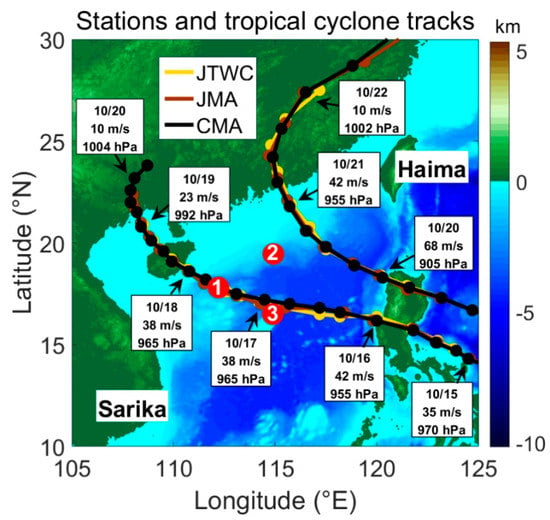
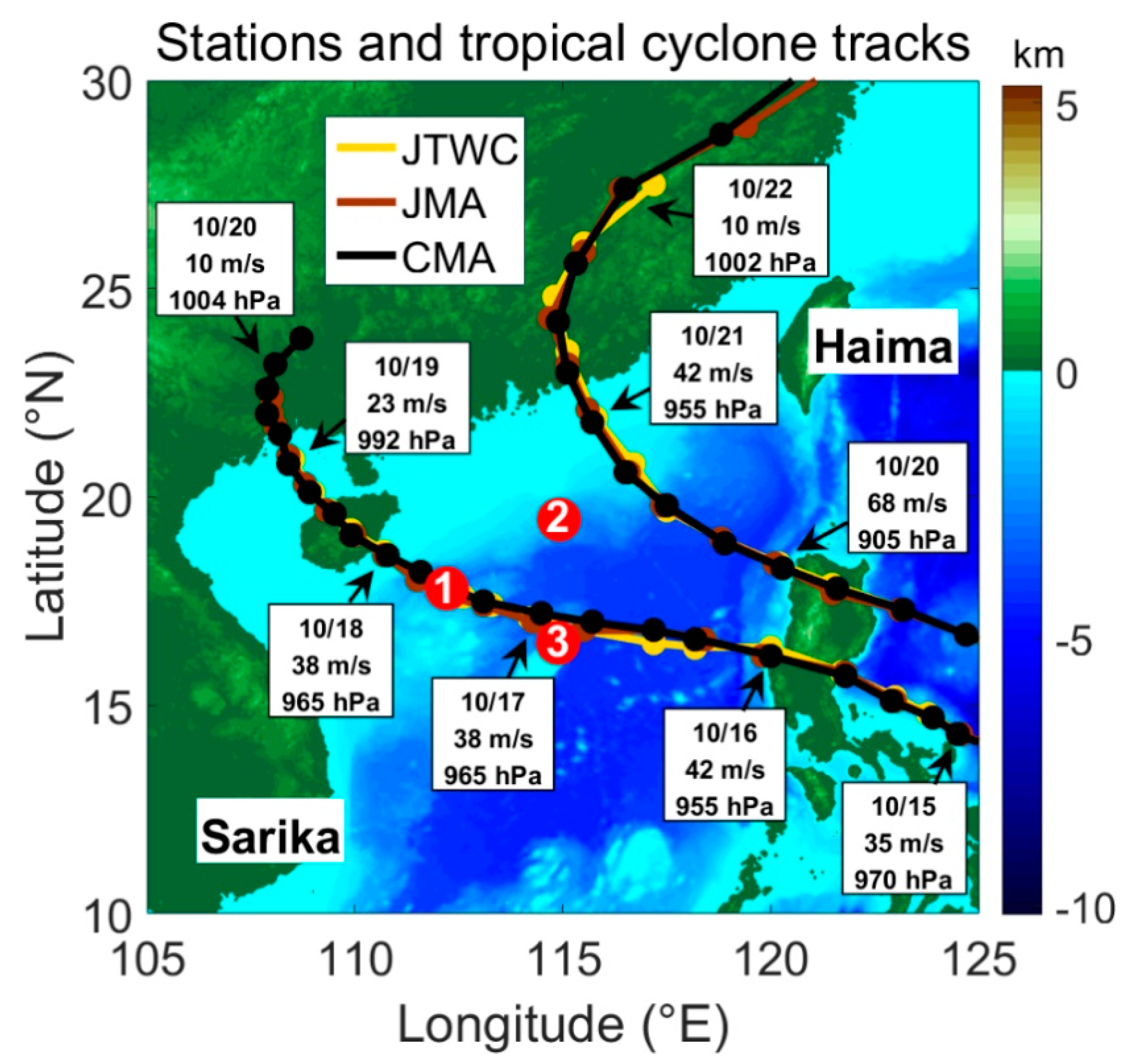
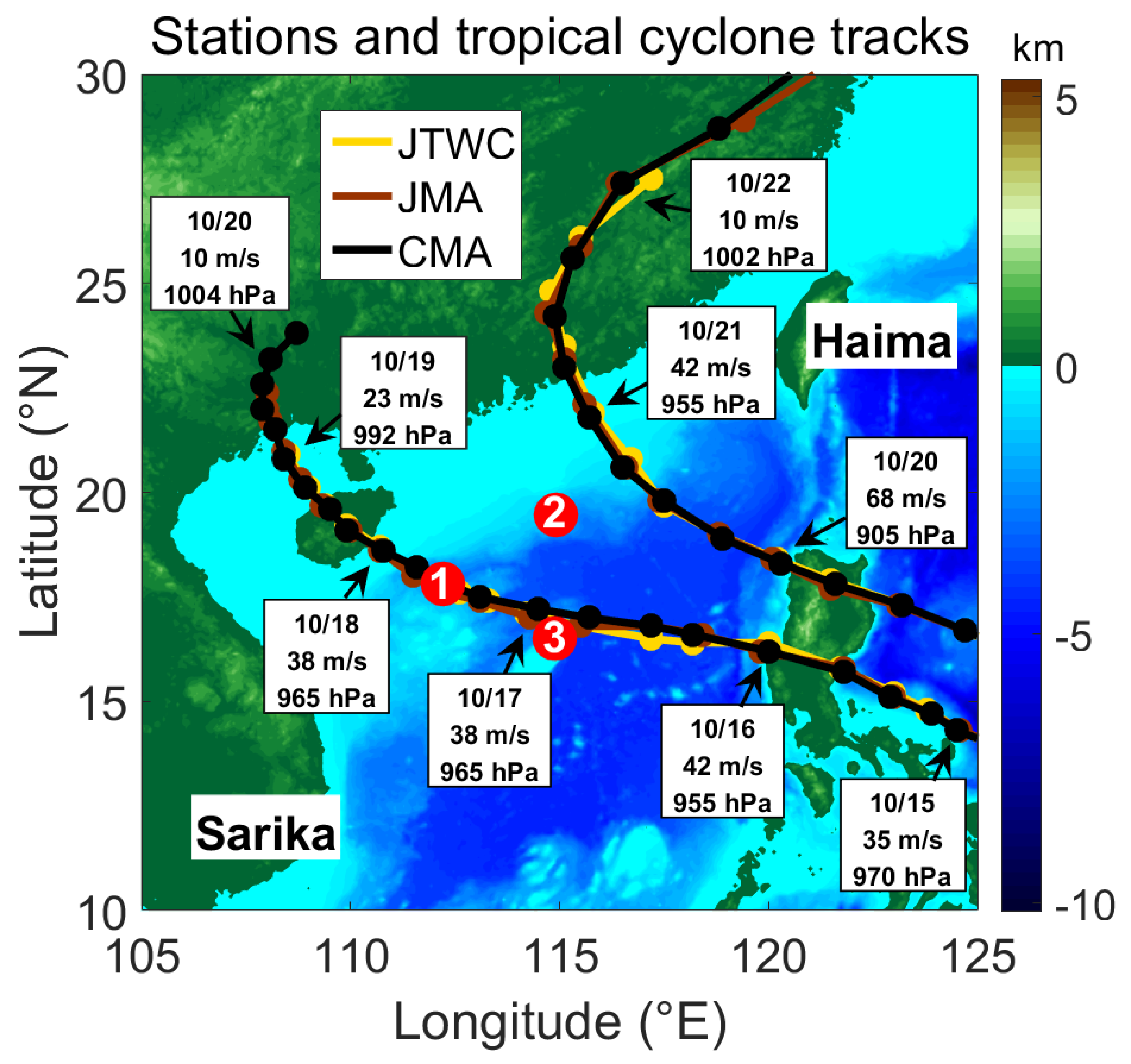
Figure 1.
Tracks of Typhoons Sarika and Haima obtained from the Joint Typhoon Warning Center (JTWC) data (orange), Japan Meteorological Agency (JMA) data (brown), and China Meteorological Administration (CMA) data (black), showing their positions every 6 h (dots). The text boxes point to the UTC 00:00 of the positions everyday, show the dates, sustained maximum wind speed, and central pressure obtained from the CMA data. The red numbers indicate the positions of the observation stations. The background shade indicates the topography.
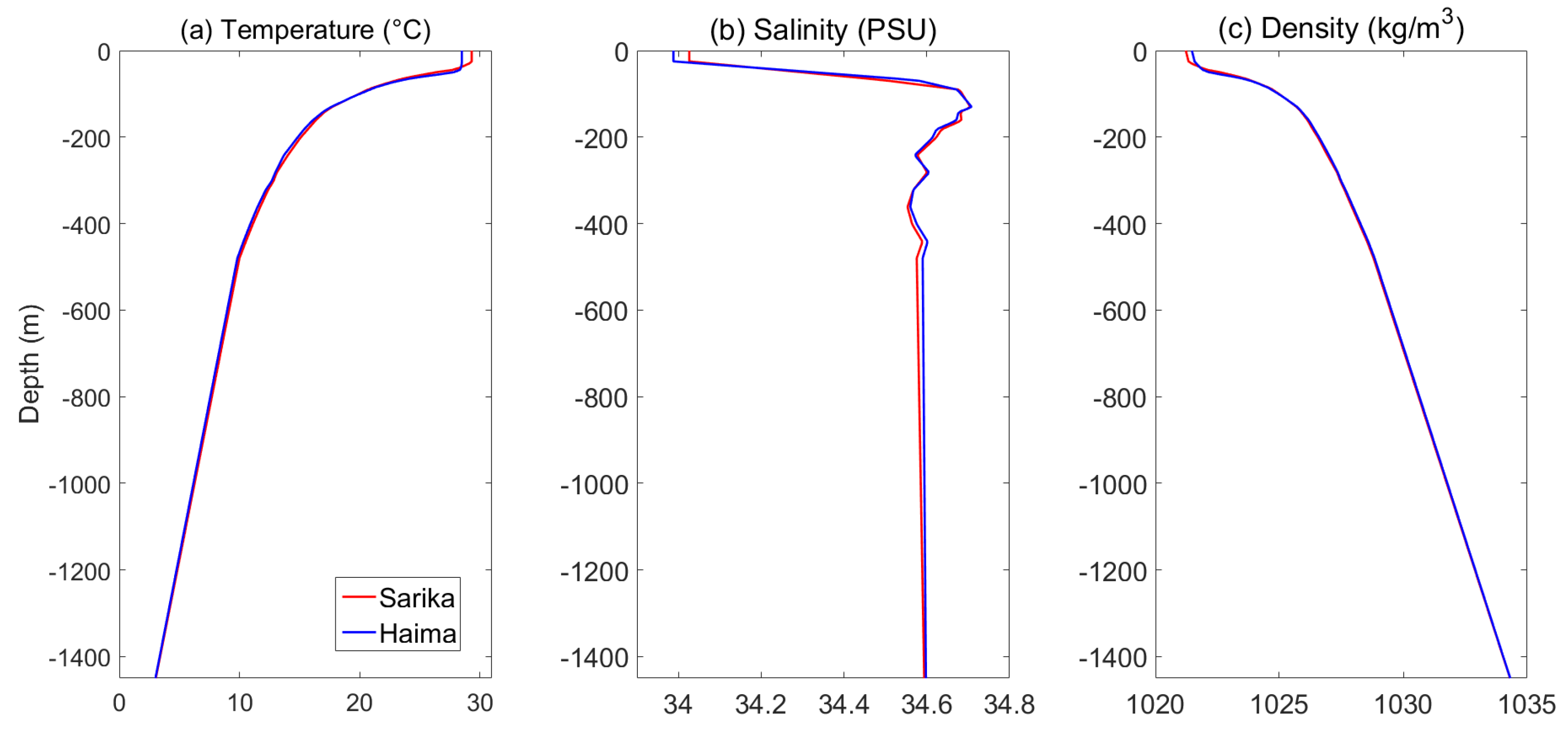
Figure 2.
Initial temperature, salinity, and density profiles for Sarika (red) and Haima (blue) in 3DPWP model simulation. Profiles for Sarika (Haima) are averaged over UTC 00:00 on 14 (16) October to UTC 00:00 on 16 (20) October of the observation at Station 2. 3DPWP: three-dimensional version of the Price–Weller–Pinkel model.
Figure 3.
(a–h) Cloud-top brightness temperatures obtained by the Himawari-8 satellite at 12:00 UTC between October 15 and 22, and (i–p) corresponding rainfall data obtained by the CPC MORPHing technique (CMORPH) data. The white hollowed dots indicate the buoy and mooring stations; the black lines indicate the tropical cyclone tracks; and the black dots indicate the centers of the tropical cyclones.
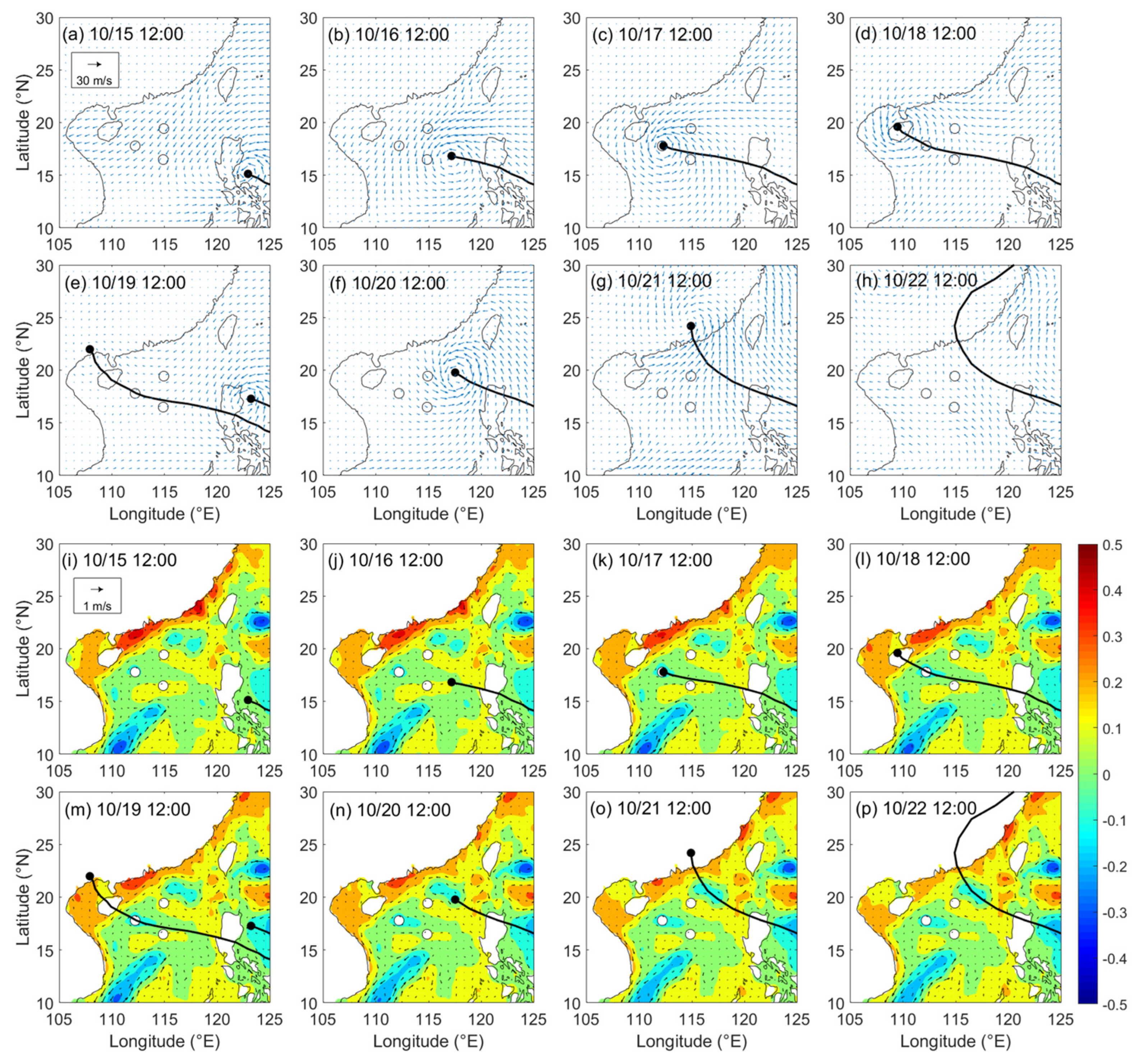
Figure 4.
(a–h) Wind data obtained by CCMP at 12:00 UTC between October 15 and 22 and (i–p) CMEMS sea surface height (color) and geostrophic current (vector) anomalies. CCMP: cross-calibrated multi-platform. CMEMS: Copernicus Marine and Environment Monitoring Service.
Figure 4.
(a–h) Wind data obtained by CCMP at 12:00 UTC between October 15 and 22 and (i–p) CMEMS sea surface height (color) and geostrophic current (vector) anomalies. CCMP: cross-calibrated multi-platform. CMEMS: Copernicus Marine and Environment Monitoring Service.
Figure 5.
(a–h) Microwave optimally interpolated (OI) sea surface temperature, and (i–p) soil moisture active passive (SMAP) sea surface salinity at 12:00 UTC between October 15 and 22.
Figure 5.
(a–h) Microwave optimally interpolated (OI) sea surface temperature, and (i–p) soil moisture active passive (SMAP) sea surface salinity at 12:00 UTC between October 15 and 22.
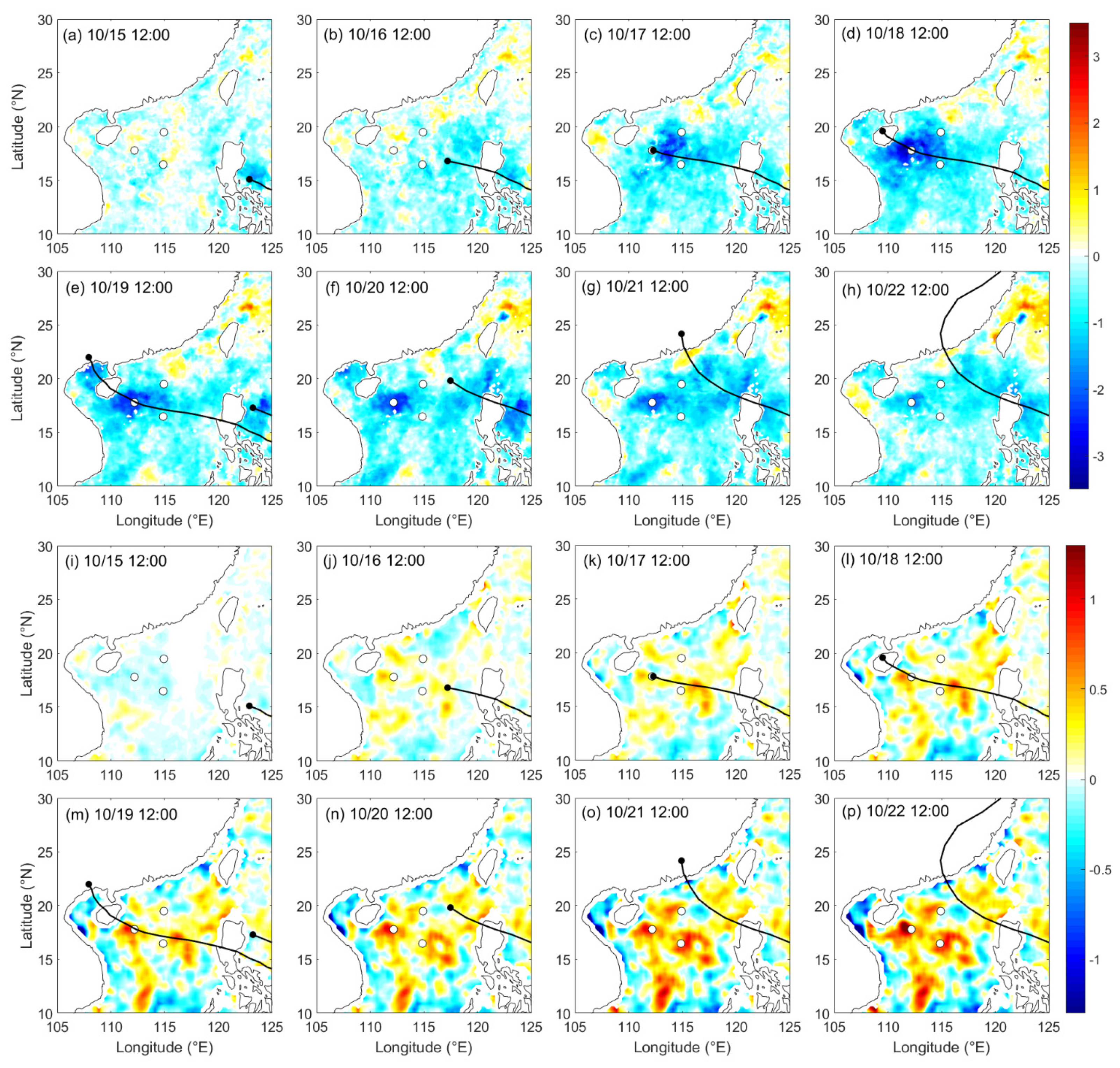
Figure 6.
(a–h) Sea surface temperature and (i–p) sea surface salinity anomalies at 12:00 UTC between October 15 and 22. The anomalies are relative to the conditions at 12:00 UTC on October 14.
Figure 6.
(a–h) Sea surface temperature and (i–p) sea surface salinity anomalies at 12:00 UTC between October 15 and 22. The anomalies are relative to the conditions at 12:00 UTC on October 14.
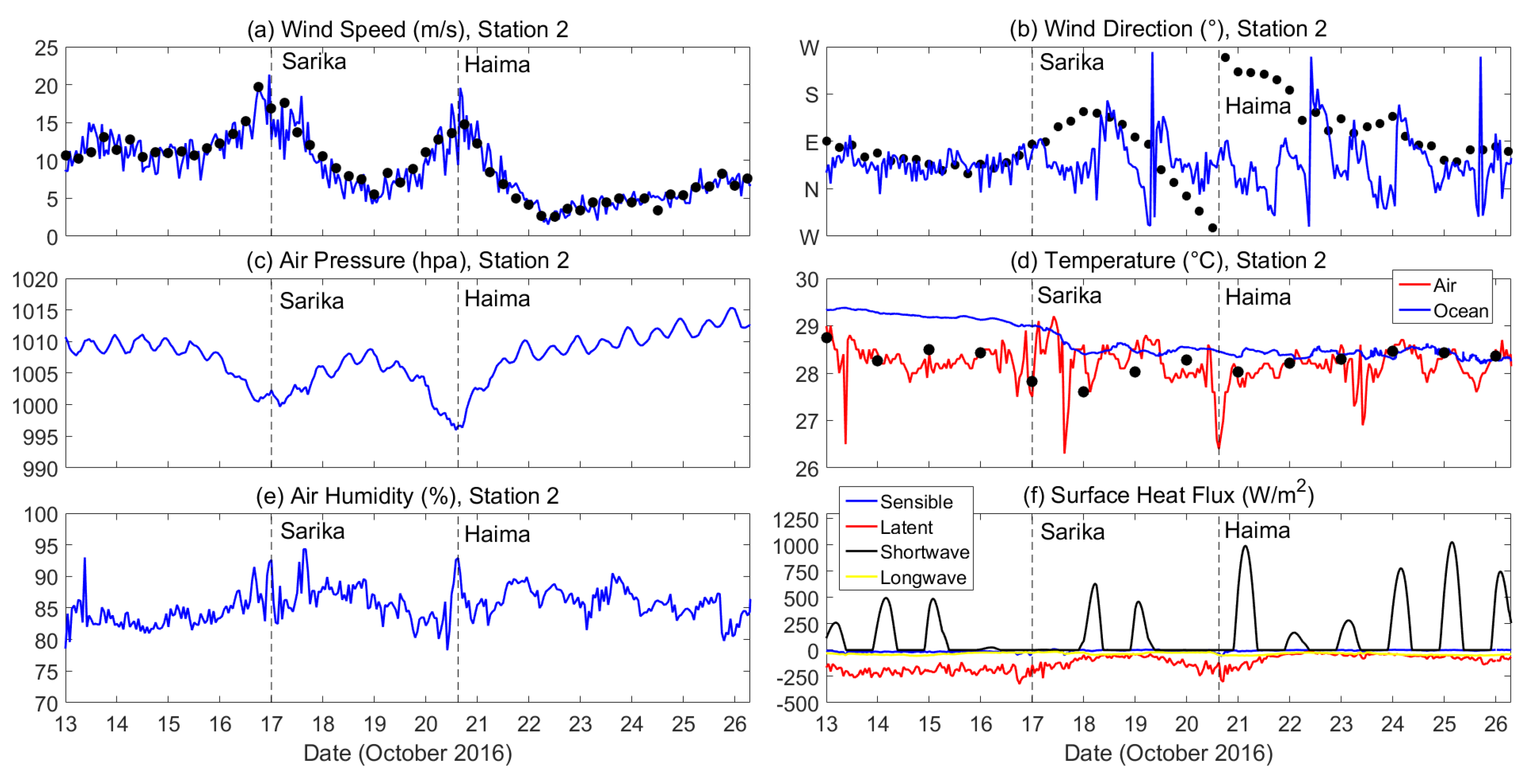
Figure 7.
Time series of the (a) sustained surface wind speed, (b) wind direction, (c) air pressure, (d, red) surface air temperature, (d, blue) sea surface temperature, (e) air humidity, surface fluxes of the (f, blue) sensible heat, (f, red) latent heat, (f, black) short wave radiation, and (f, orange) long wave radiation at Station 2 during Sarika and Haima. Regarding the wind directions, N, W, S, and E indicate the approach directions of the winds, namely, north, west, south, and east, respectively. The vertical black dashed lines represent the times when Sarika and Haima were closest to Station 2. Black dots in (a,b,d) were the remote sensingsatelliate data of cross-calibrated multi-platform (CCMP) wind and Microwave optimally interpolated sea surface temperature (OI SST).
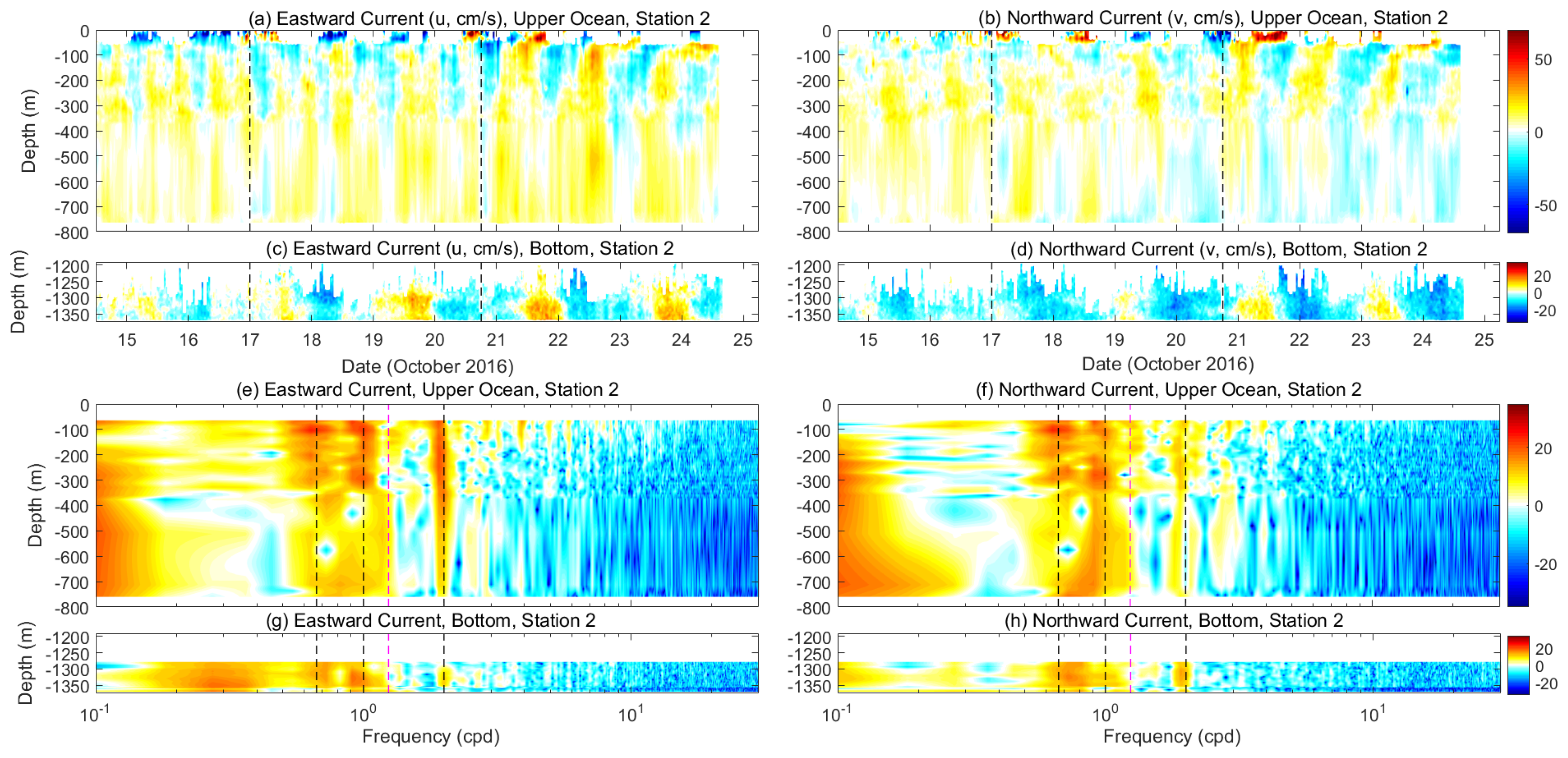
Figure 8.
Eastward and northward current (a–d) at Station 2, and their spectra between October 13 and 24 (e–h). The vertical black dashed lines indicate the inertial, diurnal, and semidiurnal frequencies. The vertical violet dashed lines indicate twice the inertial frequency.
Figure 8.
Eastward and northward current (a–d) at Station 2, and their spectra between October 13 and 24 (e–h). The vertical black dashed lines indicate the inertial, diurnal, and semidiurnal frequencies. The vertical violet dashed lines indicate twice the inertial frequency.
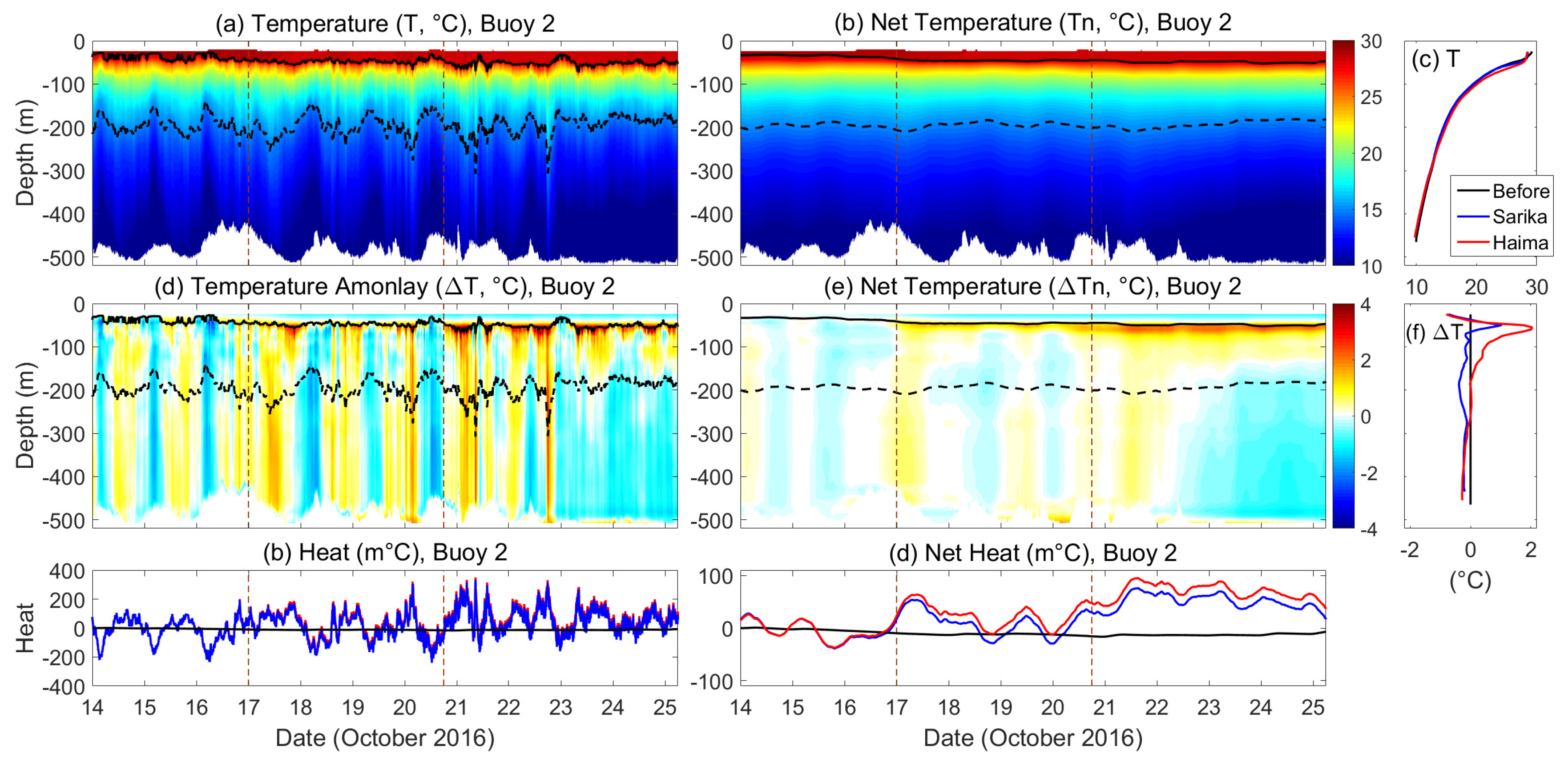
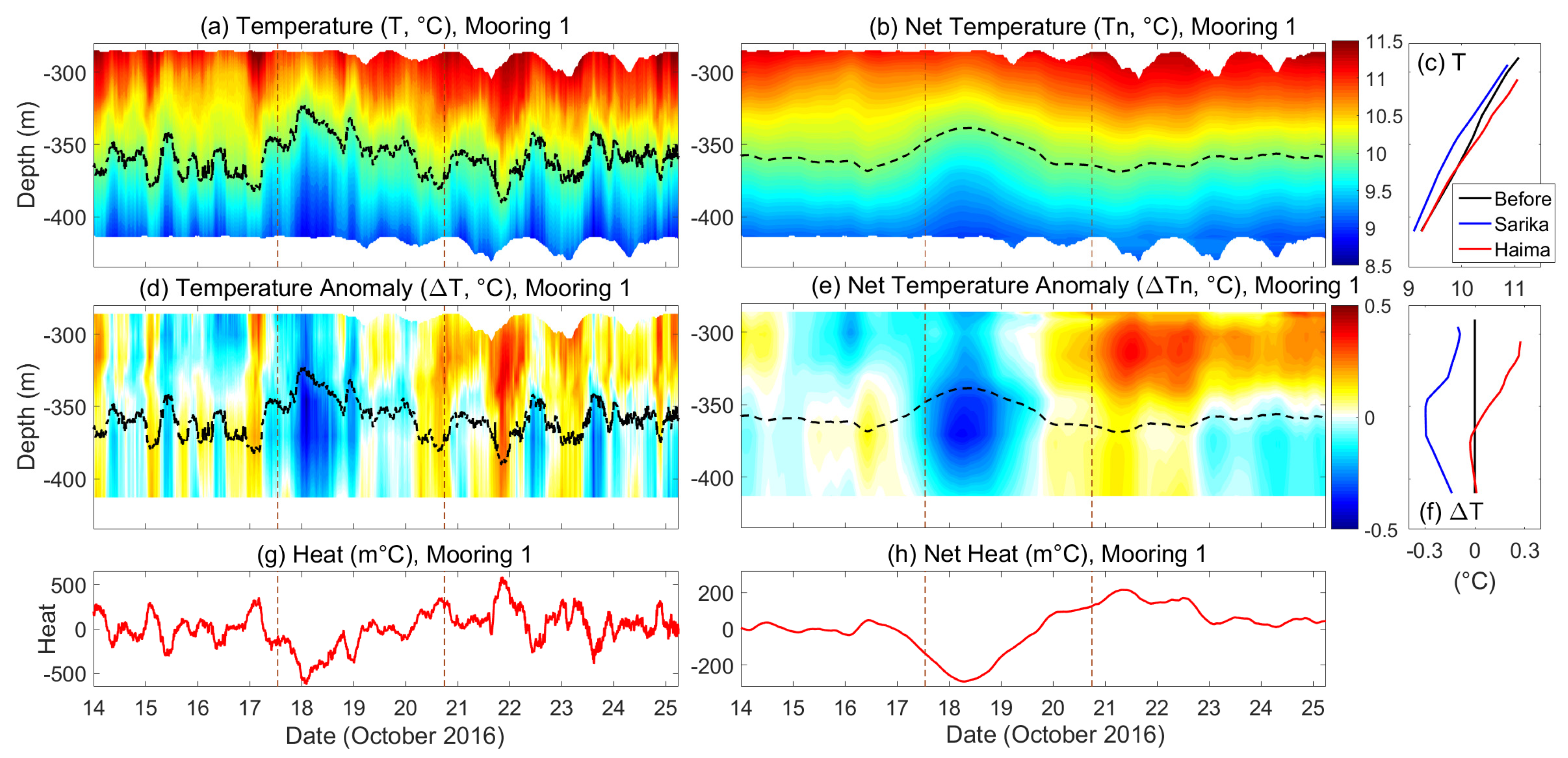
Figure 9.
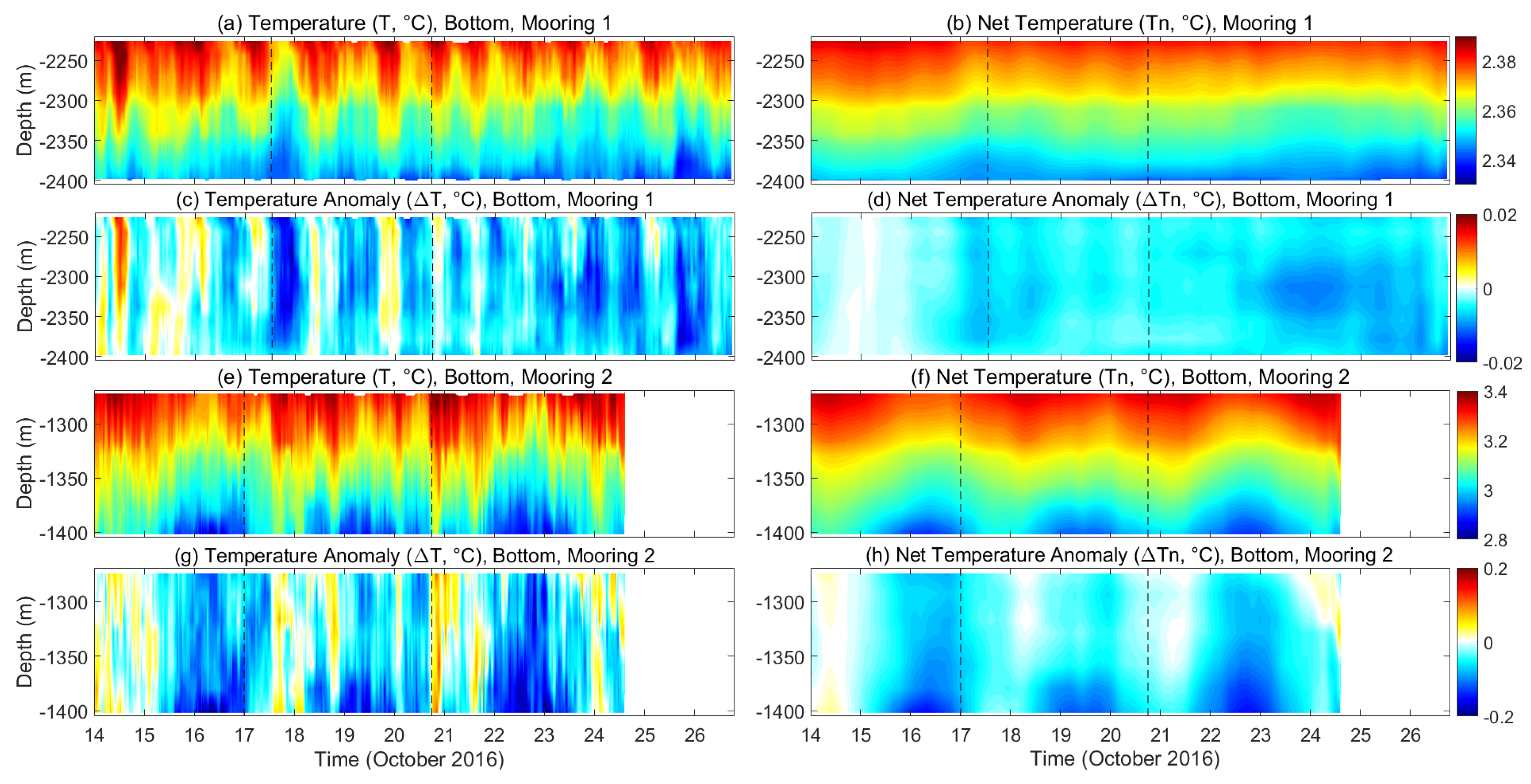
Temperature (a), temperature anomaly (d) and their net values (b,e) during Sarika and Haima at Buoy 2. Average temperature (c) and temperature anomaly (f) profiles before the two typhoons (black; averaged between 14 and 16 October), after Sarika (blue; averaged over one inertial period after 18 October), and after Haima (red; averaged over one inertial period after 22 October). The black solid lines in (a,b,d,e) indicate the mixed layer depth, which is the depth at which the temperature is 0.5 °C lower than the surface layer temperature. The black dashed lines indicate the 15 °C isotherm. (g,h) Accumulated surface heat flux (black lines), heat anomaly from 0 to 160 m (red lines), and their sum (blue lines) at Buoy 2. The vertical brown dashed lines represent the times when Sarika and Haima were closest to Station 2. The temperature observed by the sensor near the surface (at a depth of 22 m) was used for the heat content calculations for shallower depths.
Figure 9.
Temperature (a), temperature anomaly (d) and their net values (b,e) during Sarika and Haima at Buoy 2. Average temperature (c) and temperature anomaly (f) profiles before the two typhoons (black; averaged between 14 and 16 October), after Sarika (blue; averaged over one inertial period after 18 October), and after Haima (red; averaged over one inertial period after 22 October). The black solid lines in (a,b,d,e) indicate the mixed layer depth, which is the depth at which the temperature is 0.5 °C lower than the surface layer temperature. The black dashed lines indicate the 15 °C isotherm. (g,h) Accumulated surface heat flux (black lines), heat anomaly from 0 to 160 m (red lines), and their sum (blue lines) at Buoy 2. The vertical brown dashed lines represent the times when Sarika and Haima were closest to Station 2. The temperature observed by the sensor near the surface (at a depth of 22 m) was used for the heat content calculations for shallower depths.
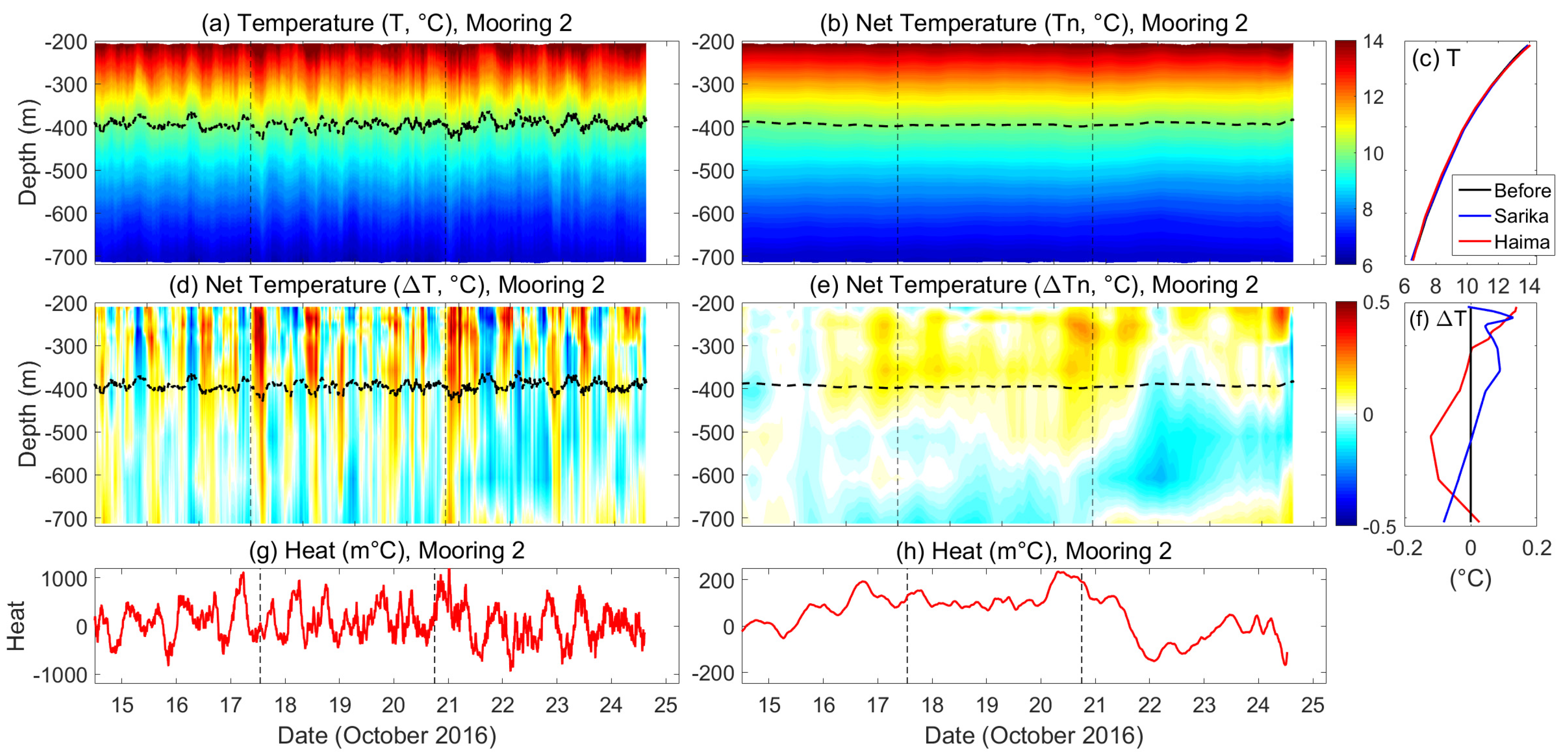
Figure 10.
Mooring 2 parameters corresponding to those in
Figure 9. The heat content anomaly and net heat content anomaly in (
g–
h) are between 210 m to 500 m in the observation (red lines).
Figure 10.
Mooring 2 parameters corresponding to those in
Figure 9. The heat content anomaly and net heat content anomaly in (
g–
h) are between 210 m to 500 m in the observation (red lines).
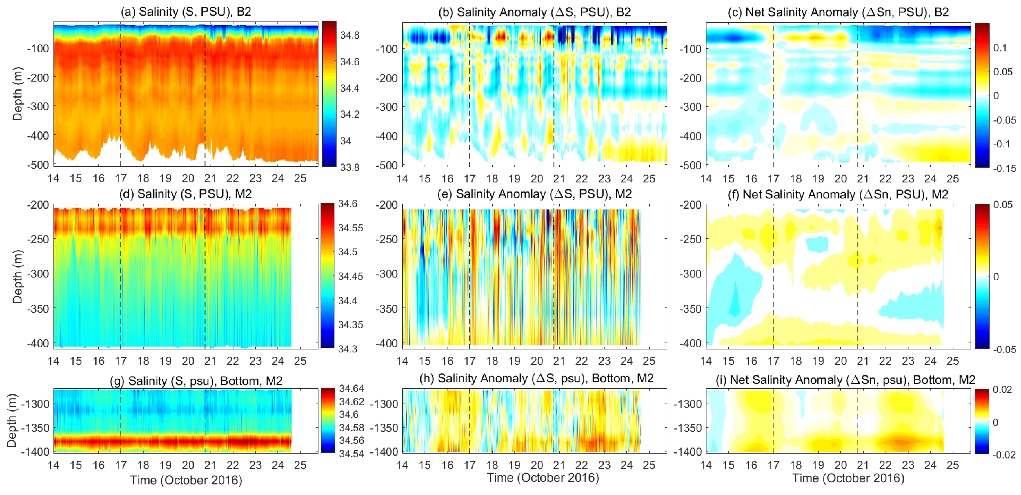
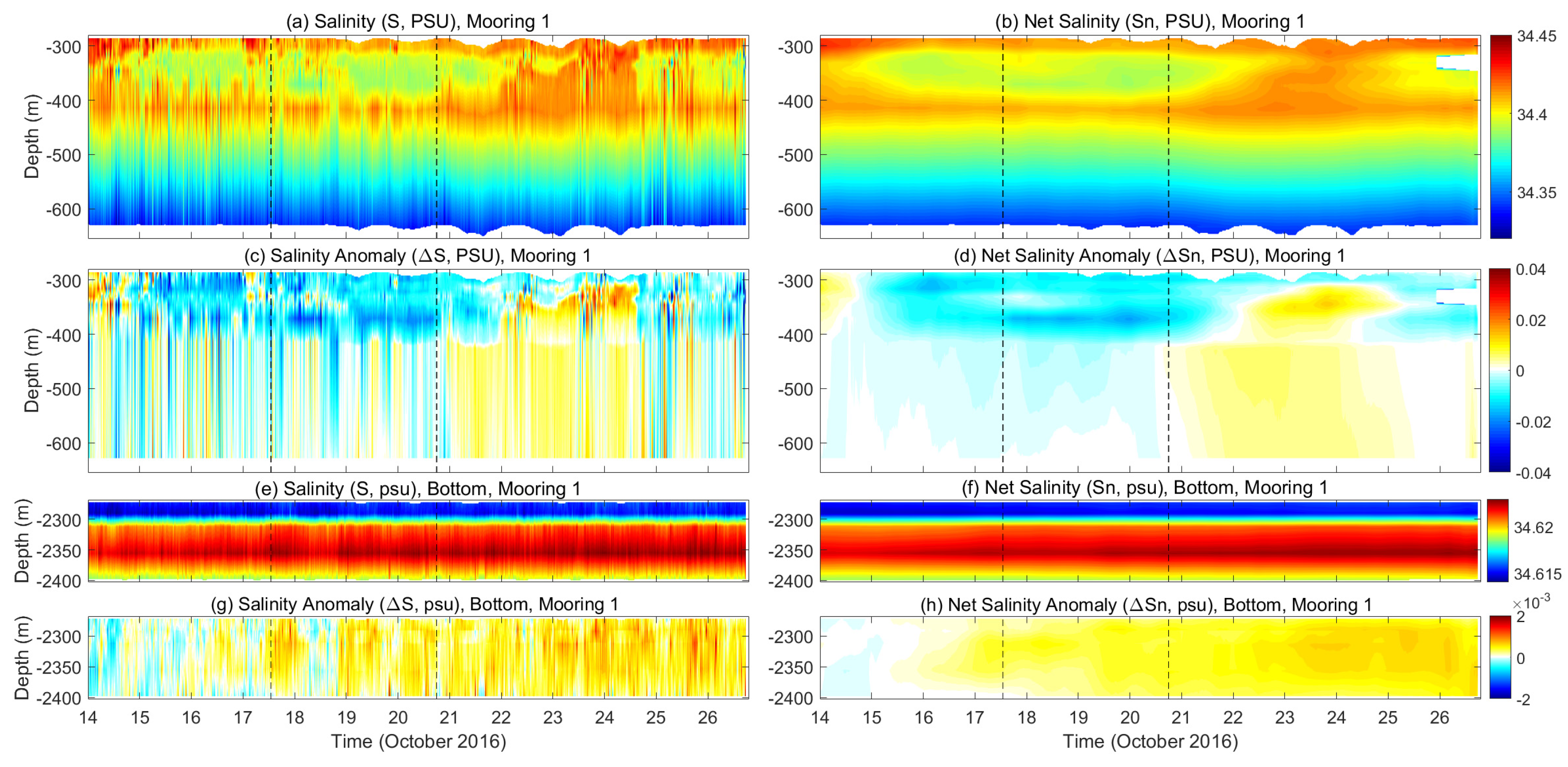
Figure 11.
Salinity, salinity anomaly, and net salinity anomaly during Sarika and Haima at Buoy 2 (a–c) and Mooring 2 (d–i). Net salinity anomaly is the one inertial period running mean of the salinity anomaly. The salinity anomaly was calculated as the salinity minus the average salinity over the period UTC 00:00 on 14 October to UTC 00:00 on 16 October. Dashed lines represent the time that Sarika and Haima were closest to the stations.
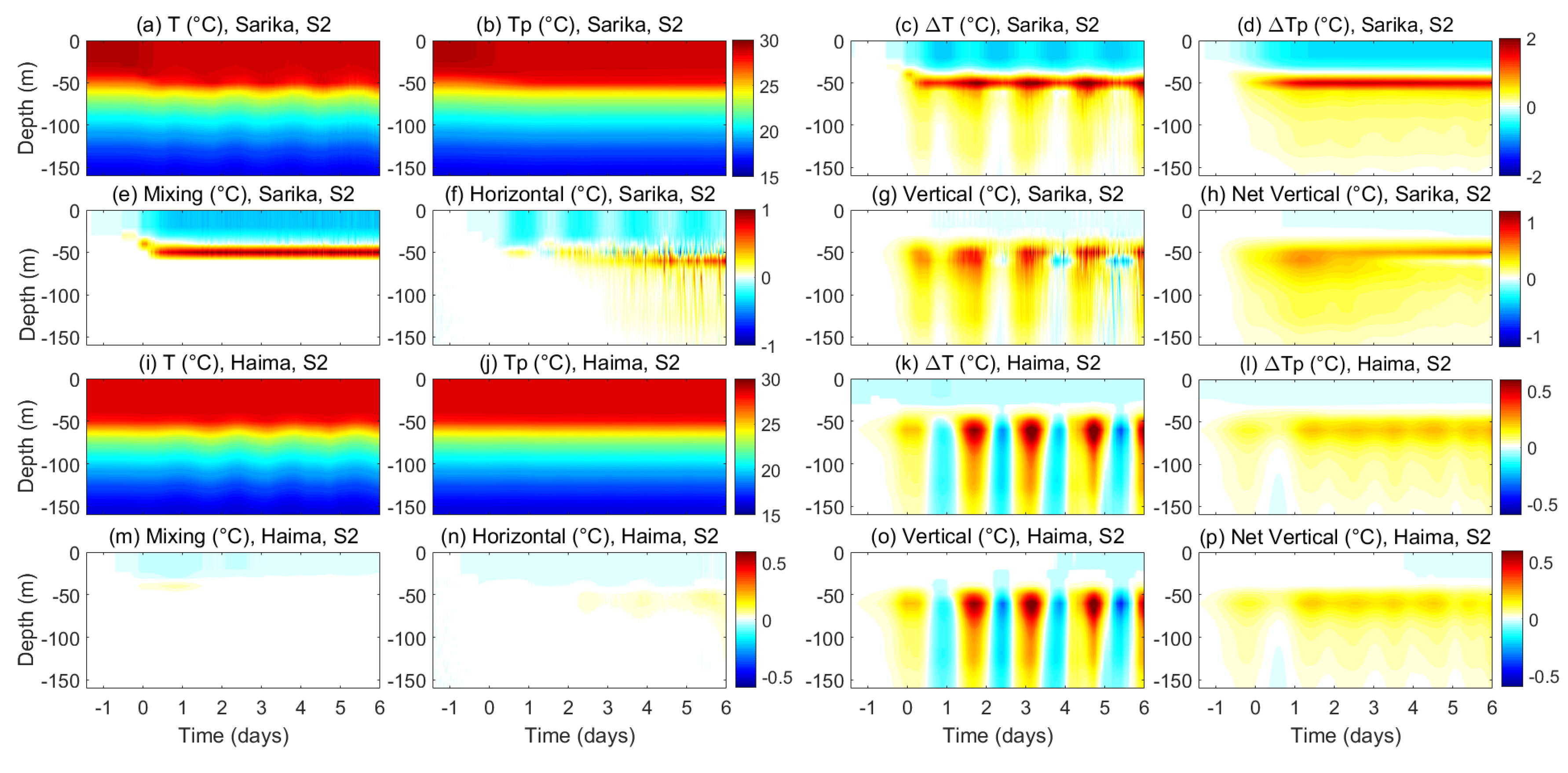
Figure 12.
Change of temperature (T), net temperature (Tp), temperature anomaly (ΔT), net temperature anomaly (ΔTp), and temperature change caused by mixing, horizontal advection, vertical advection and net vertical advection simulated by 3DPWP model during Sarika (a–h) and Haima (i–p).
Figure 12.
Change of temperature (T), net temperature (Tp), temperature anomaly (ΔT), net temperature anomaly (ΔTp), and temperature change caused by mixing, horizontal advection, vertical advection and net vertical advection simulated by 3DPWP model during Sarika (a–h) and Haima (i–p).
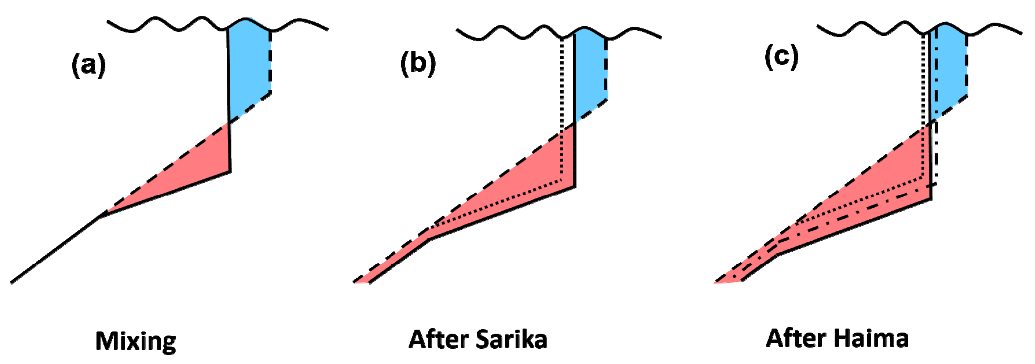
Figure 13.
Sketch of the vertical temperature profiles at Station 2 before (dashed lines) and after (solid lines) (a) only mixing, (b) Sarika, and (c) Haima. The dotted lines in (b) and (c) indicate the temperature profiles caused by only mixing, while the dot-dashed line in (c) indicates that caused by Sarika. The red shading indicates the warming anomaly, and the blue shading the cooling anomaly.
Table 1.
Sources of Data *.
Table 1.
Sources of Data *.
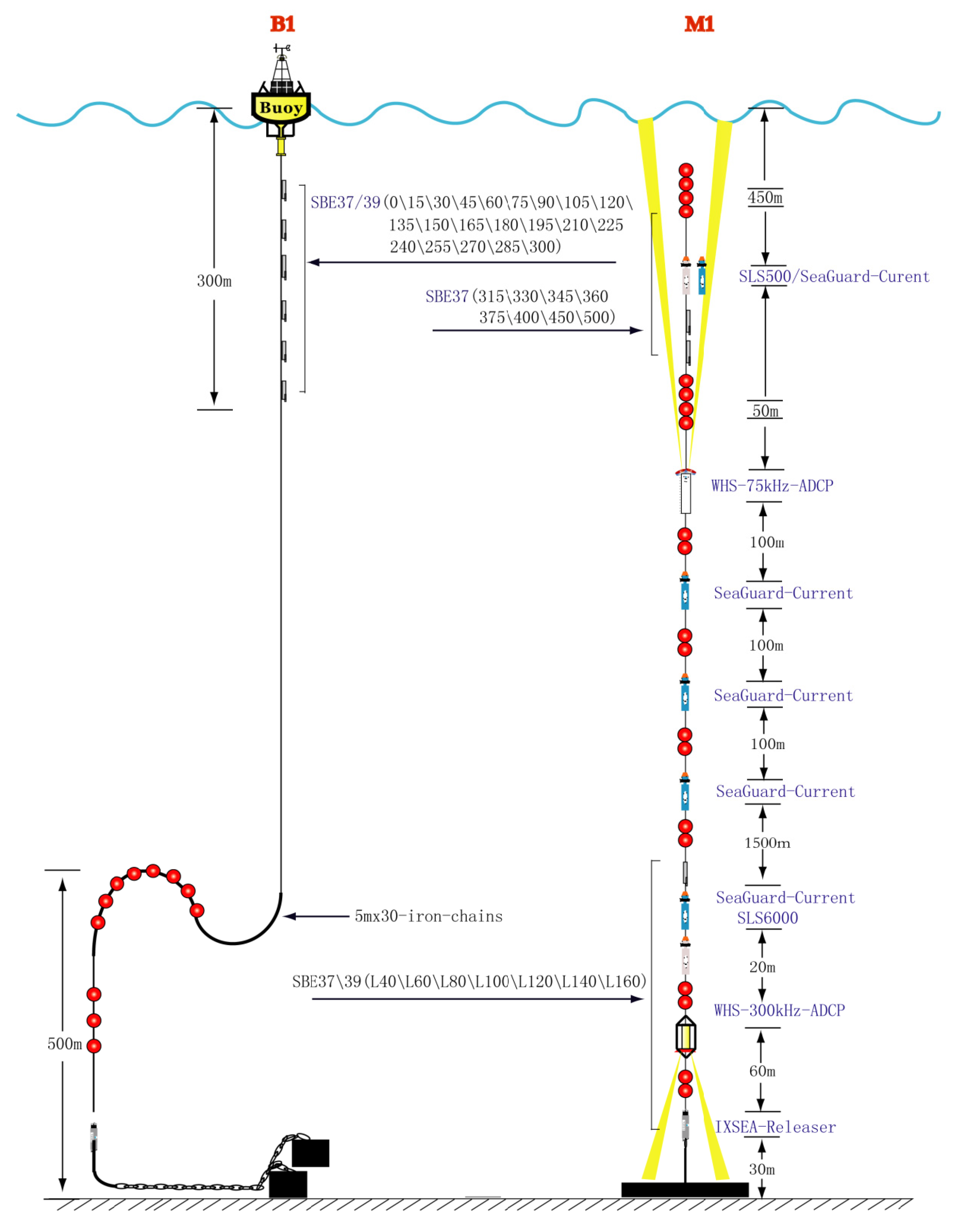
Table 2.
Observation instruments and measured elements at Buoy 2 *.
Table 2.
Observation instruments and measured elements at Buoy 2 *.
| Instruments | Measured Elements | Designed Depth (m) | Resolution (s) |
|---|
| Gill-MetPak | Meteorology | 4 m above from sea surface | 1 (3600) |
| JFE-A7CT | T, S | 12\22\52\68.5\90.5\111\131\142\162\182\202\242\282\322\362\402\442\482 | 300 |
| ONT7000 | T | 17\27.5\44\49.5\63\74\85\96\106\147\157\302\342\382\422\462\502 | 1 |
| SBE-56 | T | 33\38.5\57.5\79.5\101\116\121\126\121\126\137\152\172\192\222\262 | 1 |
| RDI 75K-ADCP | U, V | location: 133 m, uplooking; first bin: 24.74 m; last bin: 136.74 m; bin size: 16 m | 300 |
| RDI 300K-ADCP | U, V | location: 1385 m, uplooking; first bin: 15.69 m; last bin: 255.69; bin size: 8 m | 600 |
Table 3.
Observation instruments and measured elements at Mooring 2 *.
Table 3.
Observation instruments and measured elements at Mooring 2 *.
| Instrument | Measured Element | Design Installation Depth (m) | Resolution (s) |
|---|
| SBE-37 | T, S, P | 300/315/330/345/360/375/400/450/500/L160/L140/L120/L100/L80/L60/L40 | 120 |
| SBE-39 | T, P | 600/700/800 | 120 |
| Seaguard | U, V | 600/700/800/L80 | 600 |
| RDI 75K-ADCP | U, V | Location: 500 m, uplooking; first bin: 24.45 m; last bin: 600.45 m; bin size: 16 m | 600 |
| RDI 75K-ADCP | U, V | Location: L80 m, downlooking; first bin: 6.15 m; last bin: 110.15 m; bin size: 4 m | 600 |
Table 4.
Details of Typhoons Sarika and Haima when closest to Stations 1 and 2 *.
Table 4.
Details of Typhoons Sarika and Haima when closest to Stations 1 and 2 *.
| | Sarika-S1 | Sarika-S2 | Haima-S1 | Haima-S2 |
|---|
| Longitude (°E) | 112.168 | 114.907 | 112.168 | 114.907 |
| Latitude (°N) | 18.036 | 19.469 | 18.036 | 19.469 |
| Ocean Depth (m) | ~2400 | ~1450 | ~2400 | ~1450 |
| Distance to tropical cyclone track (km) | 15.77 | 254.49 | -535.57 | -208.44 |
| Closest time | 10/17, 13:00 | 10/17, 00:00 | 10/20, 18:00 | 10/20, 18:00 |
Table 5.
Parameters of Typhoons Sarika and Haima *.
Table 5.
Parameters of Typhoons Sarika and Haima *.
| | Sarika | Haima |
|---|
| Maximum wind speed (, m/s) | 38.00 | 42.00 |
| Translational speed (, m/s) | 6.53 | 7.18 |
| Radius of fastest wind (, km) | 120.0 (37.04) | 150.0 (46.3) |
| Mixed layer depth (, m) | 45 | 50 |
| Nondimensional translational speed, () | 1.161 (3.760) | 1.021 (3.308) |
| Rossby number of mixed layer current, | 0.253 | 0.257 |

 ,
, 


