Benefits of a Closely-Spaced Satellite Constellation of Atmospheric Polarimetric Radio Occultation Measurements

Abstract

The climate and weather forecast predictive capability for precipitation intensity is limited by gaps in the understanding of basic cloud-convective processes. Currently, a better understanding of the cloud-convective process lacks observational constraints, due to the difficulty in obtaining accurate, vertically resolved pressure, temperature, and water vapor structure inside and near convective clouds. This manuscript describes the potential advantages of collecting sequential radio occultation (RO) observations from a constellation of closely spaced low Earth-orbiting satellites. In this configuration, the RO tangent points tend to cluster together, such that successive RO ray paths are sampling independent air mass quantities as the ray paths lie “parallel” to one another. When the RO train orbits near a region of precipitation, there is a probability that one or more of the RO ray paths will intersect the region of heavy precipitation, and one or more would lie outside. The presence of heavy precipitation can be discerned by the use of the polarimetric RO (PRO) technique recently demonstrated by the Radio Occultations through Heavy Precipitation (ROHP) receiver onboard the Spanish PAZ spacecraft. This sampling strategy provides unique, near-simultaneous observations of the water vapor profile inside and in the environment surrounding heavy precipitation, which are not possible from current RO data.

1. Introduction

The climate and weather forecast predictive capability for precipitation intensity is limited by gaps in the understanding of basic cloud-convective processes [1]. Convection is a process by which rapidly rising buoyant air carries moisture (water vapor) from near the Earth’s surface upward, where it condenses. These convective processes are dependent on the environment, the water vapor and temperature vertical and horizontal structures in the surrounding region. Much of the water vapor resides in the 2 km nearest the Earth, the approximate top of the boundary layer, which is the layer where air motions are directly influenced by contact with the Earth’s surface. However, increasing evidence points to the control of deep convection by the relatively smaller and more variable amount of moisture above the boundary layer, known as the free troposphere. When abundant, free tropospheric moisture can strengthen convection by making the atmosphere more unstable. Horizontal transport and the mixing of nearby dry air (through a process known as entrainment) can weaken the convection, by decreasing the buoyancy [2,3]. Free-tropospheric moisture thus appears to exert significant control on the development of deep convection, producing heavy precipitation [4,5,6,7,8,9,10,11].

Currently, a better understanding of the cloud-convective process lacks observational constraints, due to the difficulty in obtaining accurate, vertically resolved pressure, temperature, and water vapor (denoted by p, T, and q, respectively) structure in and near convection. Infrared sensors, such as the Atmospheric Infrared Sounder (AIRS), provide water vapor structure outside of clouds and precipitation, but cannot estimate the water vapor inside clouds. Passive microwave (MW) sounding radiometers, such as the Advanced Technology Microwave Sounder (ATMS), operate in millimeter-wave (183 GHz) water vapor bands, which under heavy precipitation, are sensitive to the cloud top ice region [12], limiting their use in studies that require vertically resolved water vapor inside clouds. Passive MW radiometer satellite observations that operate in a longer wavelength water vapor band (near 22 GHz), such as the Tropical Rainfall Measuring Mission (TRMM), Microwave Imager (TMI) and similar passive MW sensors, provide a long record of total column water vapor data [13]. Global radiosonde data provides insitu measurements of the vertical (p, T and q) profile but are generally confined to over-land locations and collected near synoptic times. Ground-based Global Navigation Satellite System (GNSS) stations provide total column water vapor [14]—mostly over land—but do not measure the vertical water vapor profile.

In this manuscript, the radio occultation (RO) measurement concept is proposed to address these observational shortcomings [15,16]. An RO occurs when a receiver in low-Earth orbit (LEO) views a GNSS satellite (e.g., the US Global Positioning System, GPS) as it sets or rises behind the Earth’s atmosphere. The measured signal phase and amplitude are analyzed to derive atmospheric refractivity, from which profiles of atmospheric state variables (p, q and T) are derived [17]. A unique aspect of the RO is that the L-band (near 1.4 GHz) GNSS signals suffer minimal attenuation when propagating through even the most severe precipitation events. Owing to the orbital and observation geometry, these measurements represent integrated quantities along each ~150 km propagation ray-path, which is considerably coarser than the spatial scales associated with clouds. Traditionally, RO measurements are collected from GNSS receivers onboard disparate operational and research-based LEO satellites to assimilate into global numerical weather prediction (NWP) models at each update cycle. In order to maximize and homogenize the global sampling density, no particular preference is given to one location or type of weather being observed. Using common metrics such as geopotential height anomaly correlation scores, assimilation of these RO data into NWP models has been demonstrated to lead to an improved overall forecast predictive skill [18,19]. However, the ability of these same RO observations to capture dense vertically resolved (p, T and q) profiles in and near regions of heavy precipitation may provide insight to reveal the role of free tropospheric water vapor influencing underlying cloud-convective processes [20,21].

The idea of using RO for examining the thermodynamic makeup of convective clouds is not new [22,23] and has recently been summarized [24]. In this manuscript, we describe the potential advantages of collecting time-sequential RO from a constellation (or “train”) of closely spaced low Earth-orbiting satellites tracking the same transmitting GNSS satellite. This strategy is driven by the fact that in the acrossray direction, the horizontal resolution of an RO measurement is of a much finer scale than its orthogonal alongray scale, which is essentially limited only by the effective Fresnel zone of ~1 km. A ~2minute spacecraft separation between up to five small LEO satellites would enable each RO receiver to observe the same GNSS transmitter, such that successive RO ray paths are offset from the previous and lie “parallel” to one another. When the RO train orbits near a region of heavy precipitation, there is a possibility that one or more of the RO ray paths will intersect the region of heavy precipitation, whereas others would lie outside of heavy precipitation (Figure 1).

The presence of heavy precipitation can be discerned by the use of the polarimetric RO (PRO) technique, recently demonstrated by the Radio Occultations through Heavy Precipitation (ROHP) receiver onboard the Spanish PAZ spacecraft [25], which is further detailed below. This sampling strategy provides unique, near-simultaneous observations of the water vapor profile inside and in the environment surrounding heavy precipitation, which is not possible from current RO data.

Section 2 and Section 3 describe the RO measurement requirements and a proposed PRO instrument suitable for small satellite investigations, respectively. Section 4 examines several possible orbital strategies for implementing such a closely spaced RO constellation. To estimate how frequently RO measurements onboard a constellation “train” of orbiting satellites will encounter heavy precipitation in nature, orbital simulation experiments were carried out where the RO ray paths from a four-satellite constellation were superimposed on actual 30minute precipitation fields from the Global Precipitation Measurement (GPM) [26] Integrated Multi-satellitE Retrievals for GPM (IMERG) precipitation product [27].

2. RO Measurement Requirements

During an RO, the transmitted GNSS signal undergoes refractive bending, causing a phase shift in the signal due to variations of the atmospheric refractive index. Atmospheric refractivity is directly related to the density of the atmosphere (temperature and pressure) and its water vapor content. Typically, an RO receiver tracks two GNSS carrier frequencies (denoted L1 and L2) to separate the dispersive ionospheric delay from the non-dispersive atmospheric delay (refractive index-based delay induced by the tropospheric constituents). For GPS, L1 = 1.57542 GHz and L2 = 1.22760 GHz.

The key measurement required from a GNSS-RO instrument is a time series of phase delays relative to an initial arbitrary phase. Knowing the precise positions and clock drifts of the transmitter and receiver, the receiver phase delays are converted to excess phase delay due to the atmosphere as the ray paths cut through successive atmospheric layers [17]. The atmospheric refractive index is obtained successively from each layer from top to bottom, like peeling an onion [16]. The theoretical vertical resolution of the retrieval is limited by diffraction within the atmosphere and estimated to be ~60 m [24]. In practice, measurement noise limits the obtainable vertical resolution to ~200 m in the lower troposphere [28,29], providing a horizontal resolution in the range of ~100 km, sufficient for the synoptic scale structures addressed in Section 1. In the low to middle troposphere (below ~10 km altitude in the tropics), the relevant altitude range for the free troposphere, retrieval of water vapor profile requires a priori information on temperature [16,30]. Given the reasonable estimates of the temperature and refractivity uncertainties, tropospheric specific humidity can be determined to within 0.5 g/kg per profile [31,32,33].

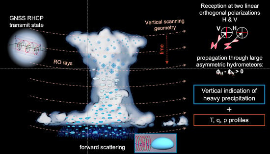
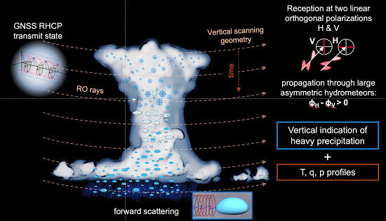
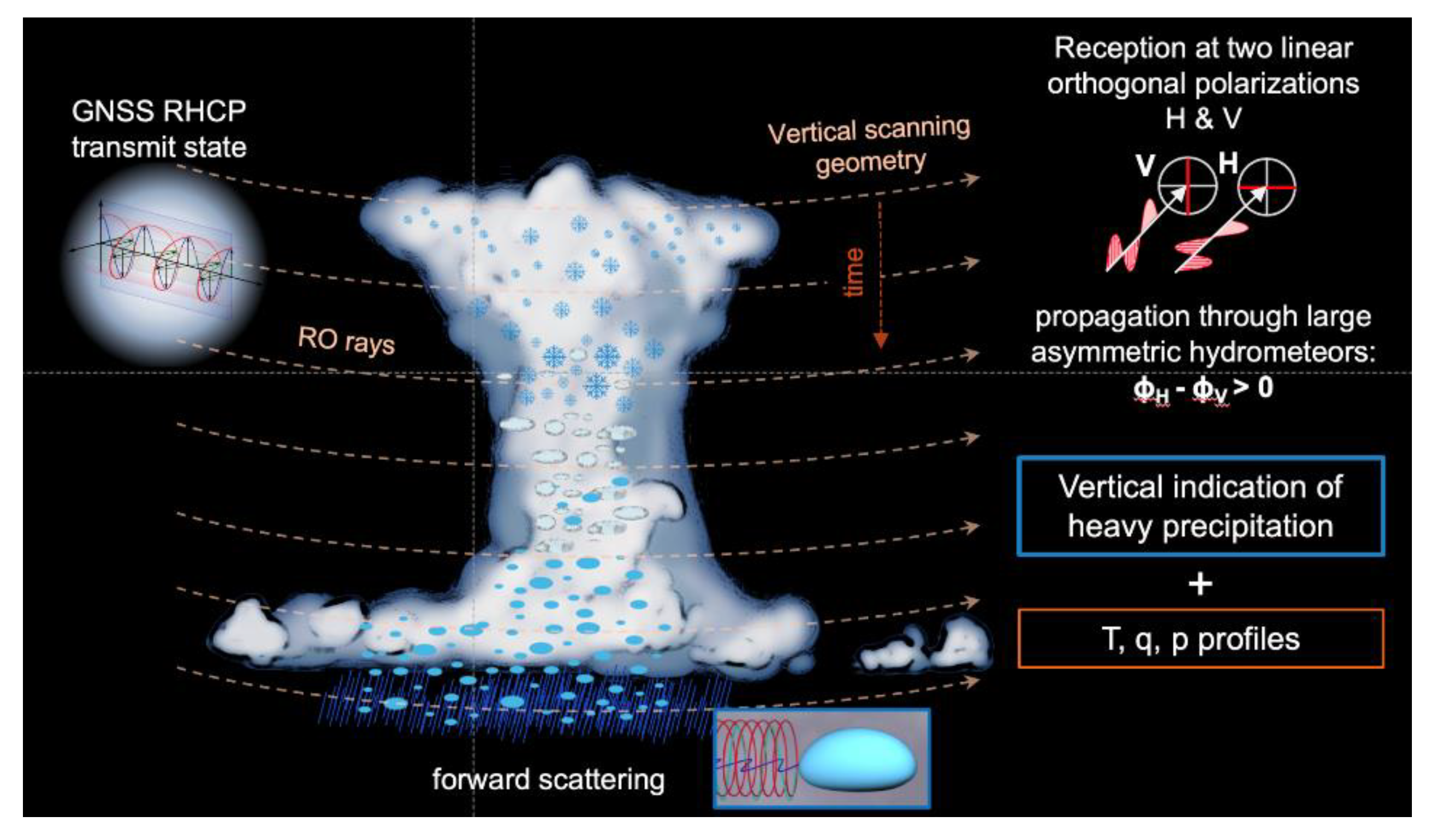
2.1. Polarimetric RO Concept

However, conventional RO provides no unique capability for distinguishing the presence or absence of precipitation along each RO ray path. A large collection of close-time coincidences of RO-based soundings with Tropical Rainfall Measuring Mission (TRMM) Precipitation Radar (PR) and CloudSat radar observations was examined by [34] to differentiate the vertical distribution of atmospheric layers stable to convection during precipitating events. In this manuscript, a combination of such RO soundings with the polarimetric RO (PRO) concept is proposed for directly distinguishing RO profiles whose propagation ray paths traverse regions of heavy precipitation (Figure 2), characterized by increasingly larger numbers and sizes of aspherical (oblate-shaped) hydrometeors as the rainfall rate increases.

PRO enhances standard RO by observing the GNSS signals in two orthogonal polarizations [35]. The co- and cross-polarized radio signals propagating through heavy precipitation media will experience different phase delays (phase delay is denoted by $\varphi$), measurable by the receiver’s polarimetric antenna. Realistic scattering simulations performed using collocated COSMIC RO and TRMM precipitation retrievals have shown that the phase difference between the horizontally (H) and vertically (V) polarized signals (defined as ${\Delta }\varphi$) is large enough to detect a path-averaged rain rate exceeding 2 mm h⁻¹ with over 70% probability [35]. The PRO concept has recently been proven by the ROHP instrument onboard the Spanish PAZ satellite launched in February 2018, a proof-of-concept experiment [25,36]. Further calibration and validation accounting for the antenna pattern, Faraday effects and other factors is detailed in [37].

As an example of ROHP data in the presence and absence of heavy precipitation, Figure 3 shows five ROHP observations (labeled A through E) on 23 May 2018 near tropical cyclone Mekunu. Large ${\Delta }\varphi$ exceeding 25 mm were obtained up to 10 km in height in regions associated with heavy precipitation surrounding the eyewall near 55E/10N (label A), whereas regions of no precipitation (labels B, C and D) exhibit no significant ${\Delta }\varphi$ anywhere in the profile. ${\Delta }\varphi$ near 10 mm (label E), associated with thin cold clouds, suggests that ROHP may also be sensitive to frozen crystalline ice shapes, similar to the differential phase observed by the ground-based polarimetric radars [38].

The locations of strong convection and associated heavy precipitation have implications for the orbital design strategy outlined in Section 3. ROHP is currently (late 2019) providing about 200 observations per day. To show geographically where the strongest observed ${\Delta }\varphi$ occur and how this correlates with known precipitation climatologies, Figure 4 shows the locations of the upper percentile (upper 2%) of ROHP observations that results after ${\Delta }\varphi$ is averaged from the RO rays whose tangent point intercepts three different vertical regions (0–5, 5–10 and 10–15 km height). The top panel includes only data from June–July–August (JJA), and the lower panel from December–January–February (DJF). The color background map depicts the average rain rate during these months derived from the GPM IMERG precipitation product. During JJA, there is a good agreement of <Δϕ> in the 10–15 km region (red symbols) with known areas of convection, notably the Maritime continent, the Pacific Intertropical Convergence Zone (ITCZ) and the African Sahel. During DJF, the maximum shifts to the Amazon and the Western Pacific Ocean. The strong precipitation in the 0–5 km layers (black colors) is not restricted to the tropics, but also captures heavy but shallow oceanic rain events below 40S latitude, and cold season precipitation poleward of 50 degree latitude (RO events poleward of 60 degrees latitude are not shown since their location lies outside the range of the IMERG product).

2.2. The Cion RO Receiver

Early RO-based satellites such as the FORMOSAT-3/COSMIC RO constellation carried the IGOR (Integrated GPS Occultation Receiver) GNSS receiver, which is based on the BlackJack receiver designed at JPL, and flown on such missions as PAZ, CHAMP, SAC-C, and GRACE. The recently deployed (June 2019) six-satellite COSMIC-2 constellation [39] carries the TriG GNSS receiver (the name implies the first letter of each of three common GNSS systems, namely GPS, Galileo and GLONASS), the follow-on to BlackJack [40]. However, IGOR or TriG are much too large to be flown on small satellites, such as a 6U cubesat.

Recently, a low-cost, low-power, and low-mass GNSS receiver (Cion) was developed at JPL [41]. The Cion receiver was designed for two commercial firms, Tyvak and GeoOptics, for use in the GeoOptics CICERO (Community Initiative for Continuing Earth Radio Occultation) constellation [42]. Cion uses a commercial off-the-shelf (COTS) computer along with existing space-qualified RF downconverters, software, and firmware to produce the precise timing needed to generate RO profiles (Figure 5). The Cion is capable of recording both setting and rising occultations, and the processing uses the open-loop (OL) tracking implemented in the receivers for COSMIC and COSMIC-2 for extended water vapor profiling through the moist lower troposphere [43]. A JPL version of the Cion receiver suitable for NASA small satellite missions has been designed and is currently being built for the SigNals of Opportunity P-band Investigation (SNOOPI) In-Space Validation of Earth Science Technologies (InVEST) mission and for the Navigation Technology Satellite (NTS-3), a technology demonstration for the next-generation GNSS transmitter. It has also been proposed for numerous other missions, primarily in conjunction with other observations that require precise time tags at the level of a few picoseconds. A follow-on NASA Instrument Incubator Program (IIP) called Genesis is building on this design to enable a next-generation GNSS reflections receiver for small satellites as well.

3. Results

To estimate how frequently RO measurements from a constellation of low Earth-orbiting satellites will encounter heavy precipitation in nature, orbital simulation experiments were carried out where the RO ray paths were superimposed on the nearest 30minute GPM IMERG precipitation product [27]. A number of different orbit scenarios were examined, varying the number of satellites, orbital altitudes and inclinations, and the relative time separation between satellites in the constellation configuration. For brevity, one such configuration (three satellites) is described in Section 3.1, with summaries of findings for other orbit scenarios described in Section 3.2.

3.1. Three-Satellite Constellation

This simulation consists of an LEO constellation of three satellites orbiting in a 45-degree inclination plane at an elevation of 500 km. The three satellites are separated by two minutes. Each satellite carries a polarimetric-capable RO receiver with a receiving antenna capable of collecting GNSS telemetry data within a 45° antenna azimuth range (relative to boresight), capable of tracking both rising and setting occultations from the GPS and GLONASS satellites. Each RO is characterized by the location of the tangent point when the straight line between the transmitter and the receiver is 100 km below the surface, corresponding roughly to a ray grazing the surface. For the purpose of this study, the choice of straight-line tangent height is unimportant since the locations of simulated RO do not depend sensitively on the height.

The RO captured by these three satellites have been simulated for 30 consecutive days and then repeated to complete a full year. A precession of −3 deg/day is included in the simulations of the satellite’s orbits to obtain a realistic sampling over the Earth. With this configuration, around 1.2E6 occultations are obtained over the course of one year. Note that this quantity stands for possible occultations, but no spacecraft duty cycle nor processing losses are taken into account. An RO event is defined as a clustered group of near-simultaneous occultations, which happen when the different satellites obtain an RO from the same GNSS transmitter. Such events can be complete (the three satellites capture an RO from the same transmitter within a few minutes), or non-complete (one or two of the three satellites miss or truncate an RO tracking opportunity). This latter condition typically happens when the transmitted GNSS ray path is oriented in such a way that it is received near the edge of the antenna pattern (e.g., >45° antenna azimuth), and the occultation falls outside the azimuth cutoff threshold, as implemented in the occultation scheduler. Considering events instead of individual ROs, over one year, 400,000 events are captured, and 97% of these are complete events (i.e., all three satellites capture an RO from the same GNSS transmitter).

A sample of where these clusters of RO appear when projected onto the Earth is shown in Figure 6, where only those RO events that have crossed the extreme precipitation are shown. Heavy and extreme precipitation is defined when the cumulative differential phase shift (defined as ${\Delta }\varphi$) exceeds 2 mm and 6 mm, respectively (discussed further in Section 3.1.1). In this one-day scenario, 1173 (about 0.1% of the total) events are shown. Note that the RO locations from this train of satellites tend to clump together, increasing the likelihood that one or more observations fall inside and outside the regions of heavy precipitation.

Further analysis of Figure 6 shows that this configuration yields events with different RO orientation geometries. Depending on the location of the transmitter and the azimuth at which the signal arrives to the receiver, the separation distance between the three RO tangent points can change, as well as the time difference separating each of the ROs. This condition can be exploited to achieve sampling of convection and its environment over a range of separations. The distribution of these separations is further explored in Figure 7. Figure 7a shows the frequency distribution (histograms) of the distance between the RO tangent points obtained by two different combinations of satellites in the train (first versus second and first versus third), and Figure 7b shows the histogram of the corresponding time difference. It can be seen how the most frequent distance separation between the first and the third RO lies around 100 km for the consecutive satellites, and around 200 km for the furthest ones, although these separations are distributed over a wide range of distances.

A similar situation happens with the time separation. Notice that although the time separation between the satellites is two minutes, the time difference between the corresponding acquired RO is not necessarily two (or four for the ones in the edges) minutes, due to the relative motion between the GNSS and the receiving satellites. The most frequent time difference between the first and the second is around 140 s, while between the first and the third RO is around 280 s.

3.1.1. Representation of Precipitation at RO Observation Times

Superimposing the RO events simulated above on actual coincident precipitation data allows for a physically realistic characterization of the number of cloud structures associated with heavy precipitation that will be sampled per year, such that the constellation will be able to provide RO soundings inside and nearby heavy precipitation almost simultaneously. Following the detectability threshold proposed by Cardellach et. al. [35], a precipitation detection threshold of ${\Delta }\varphi$ > 1.5 mm is set. This detection threshold has been confirmed with ROHP data as a conservative threshold for rays with a tangent point height of ~2 km [25,37]. In Padullés et. al. [37], detectability was defined as vertical averages of ${\Delta }\varphi$, but since IMERG is providing only surface precipitation, for the purpose of this study, a single ray close to the surface is assumed to represent the precipitation conditions at the time of the RO.

In the following discussion, the definition of “outside precipitation” is better expressed as “undetected precipitation” (i.e., when ${\Delta }\varphi$ < 1.5 mm) for the purposes of this study. This is because one is not able to completely rule out the possibility that there is precipitation present when the ${\Delta }\varphi$ that is induced is below the instrument detectability threshold [37].

For the computation of the full end-to-end contributions to ${\Delta }\varphi$ along each ray path, [36] carried out scattering computations using the T-matrix approach for liquid- and solid-phase precipitation. Since IMERG only provides surface precipitation, to calculate the precipitation-induced ΔΦ in a computationally efficient fashion, a simplified power-law equation that relates the rain rate (R) to the specific differential phase shift ($K_{DP}$) at the GNSS L-band frequency (1.575 GHz) was derived [44] and is as follows:

$$K_{DP}=c{R}^b$$

(1)

where c = 0.00868 and b = 1.218, R is in mm hr⁻¹ and $K_{DP}$ is in units of deg km⁻¹. The rain rates provided by IMERG are interpolated into the representative RO ray, which is simulated by a straight line of 300 km (i.e., 150 km on either side of the tangent point in the azimuthal direction between the GNSS satellite and the RO receiver). K_DP is integrated along the ray path to obtain ${\Delta }\varphi$.

To use a single straight-line ray is a simplification of the actual ray paths that result as the receiving and transmitting satellites occult each other. In reality, the set of RO rays do not create a perfect vertical plane while descending deeper into the atmosphere, but rather a slant collection of rays that follow the geometry created by the relative motion of the receiver with respect to the transmitter. In Figure 8, an RO event captured by three satellites is shown in Figure 8a, where two of the observations intersect precipitation, while the third is sounding outside of the precipitation structure.

A realistic representation of the RO ray projection onto the Earth surface is shown in Figure 8a (colored collection of rays), in addition to the simplified 300 km ray for each RO (black dashed line). The realistic rays are generated using actual ray-tracing from the retrievals of a real RO observation that occurred in a different location and time, and have been transported here for illustration purposes. Only the portion of these rays that lie below 6 km are shown, which are the portions that are more likely to be affected by precipitation. Therefore, the shortest colored rays (in this case, the ones closer to the N-W corner of Figure 8) represent the highest rays (shorter portions of them are below 6 km), while the longest represent the rays closer to the surface (Figure 9).

Another quantity to take into consideration is the angle between the projection on the surface of the along-ray direction and the line joining the different satellite tangent points (α). In the right panels of Figure 8, this angle α is defined as the angle between any of the dashed lines and the gray line. The top and bottom right panels in Figure 8 (Figure 8a,b) highlight the importance of such an angle: in the top panel, α is around 90° and the distance between the rays remains similar to the distance between tangent points, while in the bottom panel, where α < 10°, the effective distance between rays is significantly reduced. Such effective distance is defined as the distance between rays following a perpendicular line:

$$d_{eff}=d\cos \left(90-\alpha \right)$$

(2)

where d is the distance between tangent points.

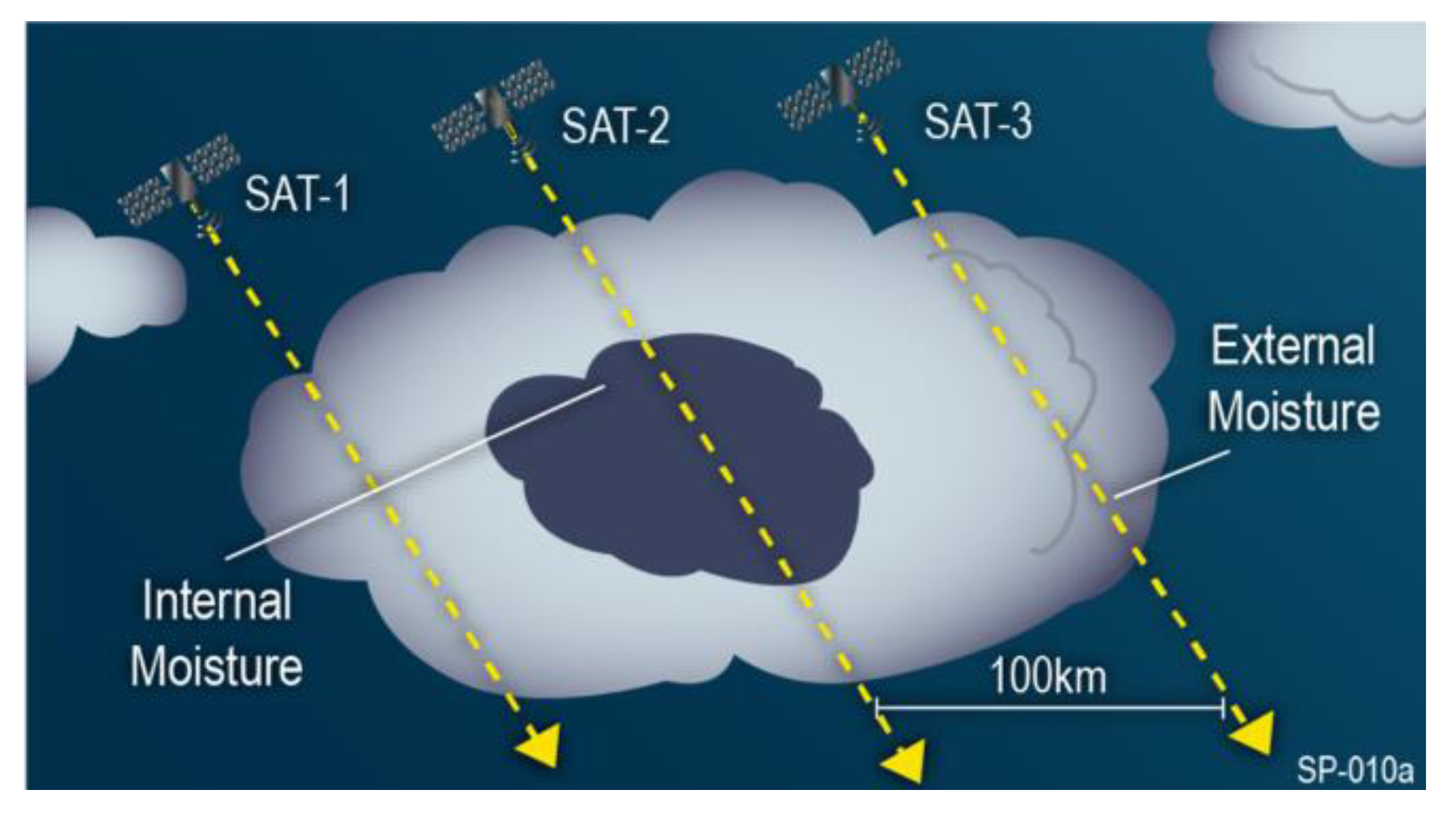
3.1.2. Near-Simultaneous RO Inside and Outside of Heavy Precipitation

The example presented in Figure 8 highlights the case where there is (at least) one RO sounding inside heavy precipitation and (at least) one sounding outside, the occurrences of which permit the analysis of relationships between soundings inside heavy precipitation and in its immediate environment. For assessing the probability of this condition across a one-year period, there are 21,500 events where at least one of the observations crosses detectable precipitation, and 15,500 that have at least one observation crossing detectable precipitation and one crossing undetectable precipitation. While scientific inferences regarding the vertical moisture structure can be gathered from the events where all soundings are inside precipitation, for this study, we are primarily focused on the events with (at least) one RO sounding inside heavy precipitation and (at least) one sounding outside. The distribution of the distances between the observations with these desired observing conditions is shown in Figure 10.

The joint distribution in Figure 10a exhibits a bimodal shape, arising from the fact that the constellation consists of three satellites. Therefore, the occurrences of sounding inside and outside precipitation can come from two consecutive satellites (e.g., RO-1 and RO-2), or the leading and trailing satellites (RO-1 and RO-3). Along with the histogram of the distance separation in Figure 10b, the histogram for α is plotted in Figure 10c. For this orbit configuration, most of the observations are confined within 20° < α < 160°.

3.2. Other Orbit Constellation Scenarios

In the discussion in Section 3.1, the 3-satellite orbit simulation was done for a non-sun-synchronous orbit with a 45° inclination plane. In this section, simulations are carried out with a 98° (sun-synchronous) orbit inclination and a 45° non-sun-synchronous orbit, each with four receiving satellites, each separated from its neighbor by two minutes. For both cases, the corresponding precession is included. These four satellites have their own location, identified as 1, 2, 3 and 4. To examine the quantity of events that will be obtained meeting the “at least one RO inside and at least one RO outside” criteria defined above, different configurations of the four satellites are considered. For example, the configuration whereby all four satellites are considered is identified as “1-2-3-4” and the separation distance is always two minutes. If only the first and third satellites are considered, the configuration is denoted by “1-3” and the separation distance is 2 + 2 = 4 min, etc.,

Table 1. Six different orbital scenarios summarized in Figure 11. Each row in the table corresponds to the same row in Figure 11.

Name	Satellite Configuration	Orbital Depiction	Separation (min)
1	1-2	⚫ ⚫ ◯ ◯	2
2	1-3	⚫ ◯ ⚫ ◯	4
3	1-4	⚫ ◯ ◯ ⚫	6
4	1-2-3	⚫ ⚫ ⚫ ◯	2, 2
5	1-2-4	⚫ ⚫ ◯ ⚫	2, 4
6	1-2-3-4	⚫ ⚫ ⚫ ⚫	2, 2, 2

lists the six scenarios.

The total number of cases that have at least one observation crossing detectable precipitation and one crossing undetectable precipitation and the distance between the tangent points d, is computed for six prescribed configurations. These results are depicted in Figure 11 (d in grey box and d_eff as a blue line). The left and right columns refer to the 45- and 98-degree inclination scenarios, respectively, and each of the six rows corresponds to the row in Table 1.

The first thing to notice is that the total number of cases increases with the number of satellites, but also with the maximum time separation between these satellites. This is a direct consequence of having more chances of hitting precipitation by increasing the number of satellites (i.e., number of observations) and increasing the likelihood of observing simultaneously inside and outside the precipitation structures by increasing the nominal separation. In general, there are more cases of simultaneous inside and outside precipitation observations with the 98° orbit configuration, since the separation between the observations is larger.

It is also noticeable how the distribution of effective distances changes with respect to the distances between the tangent points. However, the cases where d_eff > 25 km is more than the 85% of the total cases for all configurations. The d_eff is remarkably similar to the distance between tangent points for the cases with an orbital plane of 98°. The reason is that for this configuration, α is closer to 90°. This is a consequence of the orbit inclination, and the relative inclination between the GNSS satellites and the receiving satellites. For such a configuration, most of the occultations are collected at the edges of the receiving antenna beam pattern (i.e., away from the velocity or anti-velocity direction of the receiving satellite), while for the 45° inclination orbit, the observations are more likely to be collected with the central part of the antenna beam pattern (RO geometry more aligned with the velocity or anti-velocity direction of the receiving satellite). Besides the changes in d_eff, this also means that the observations collected with the 98° orbit configuration can suffer from a larger tangent point drift and its derived uncertainties [45].

4. Discussion

For these orbit simulations, two different orbital planes were considered. The study first examined the RO sampling conditions from a 3-satellite LEO constellation orbiting in non-sun-synchronous 45° inclination plane, where each satellite is separated by 2 min. To assess how the RO sampling from this low inclination differs from the sampling conditions of the more common polar (98° inclination, sun-synchronous) orbit, a 4-satellite LEO constellation was simulated for both inclinations, all other aspects being the same. These simulations showed that:

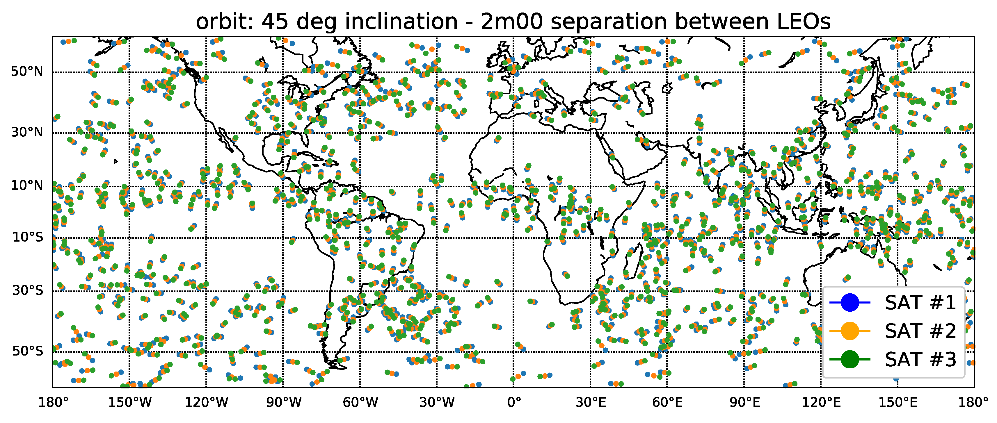
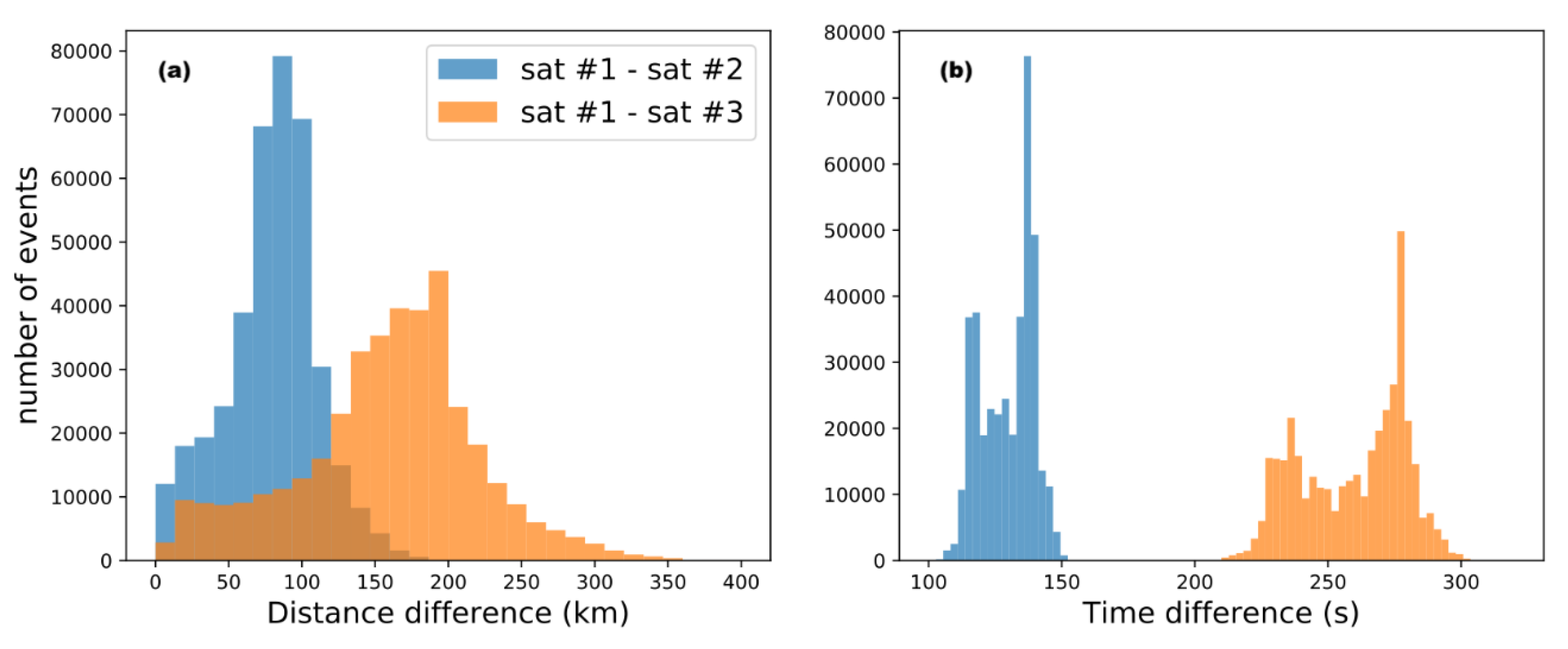
• Over one year, a 3-satellite constellation 45° inclination plane will collect 400,000 events and 97% of these are complete events (i.e., all three satellites capture a RO from the same GNSS transmitter).
• Of these complete events, the superposition of GPM IMERG data reveals that 15,500 will have at least one observation crossing detectable precipitation and one crossing un-detectable precipitation.
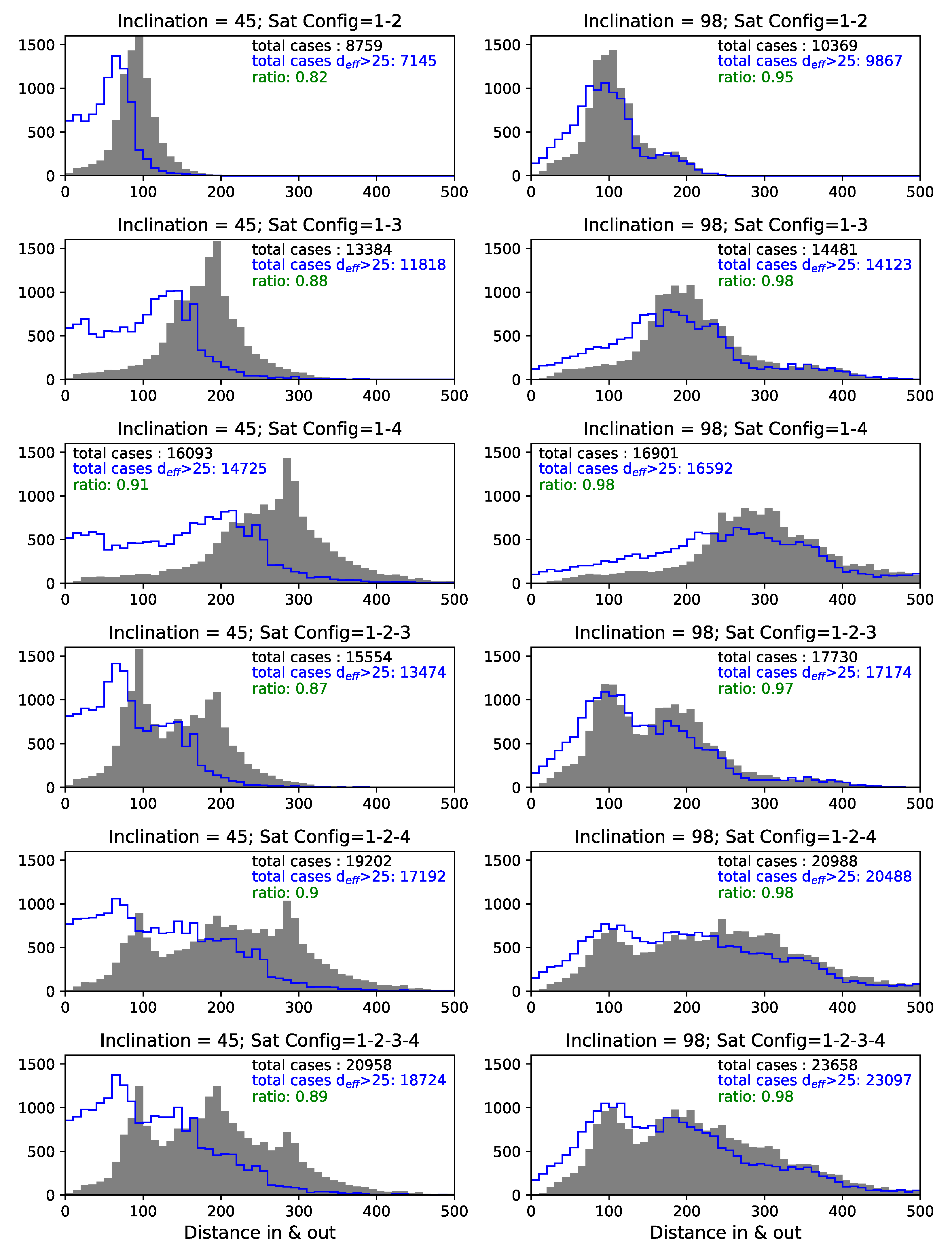
• The 98° orbit resulted in more events meeting the criteria in (2) above than the 45° inclination orbit, because there is more distance separation between the RO observations. However, the relative inclination with the GPS and GLONASS satellites also makes these observations more likely to have α ~90° deg, and hence smaller d_eff distances. From a scientific standpoint, it is better to have smaller distances to be able to characterize the convection inside and in the nearby environment (too far apart is less desirable). With this rationale, the 98° orbit is less optimal for the study of the immediate surrounding of precipitation.
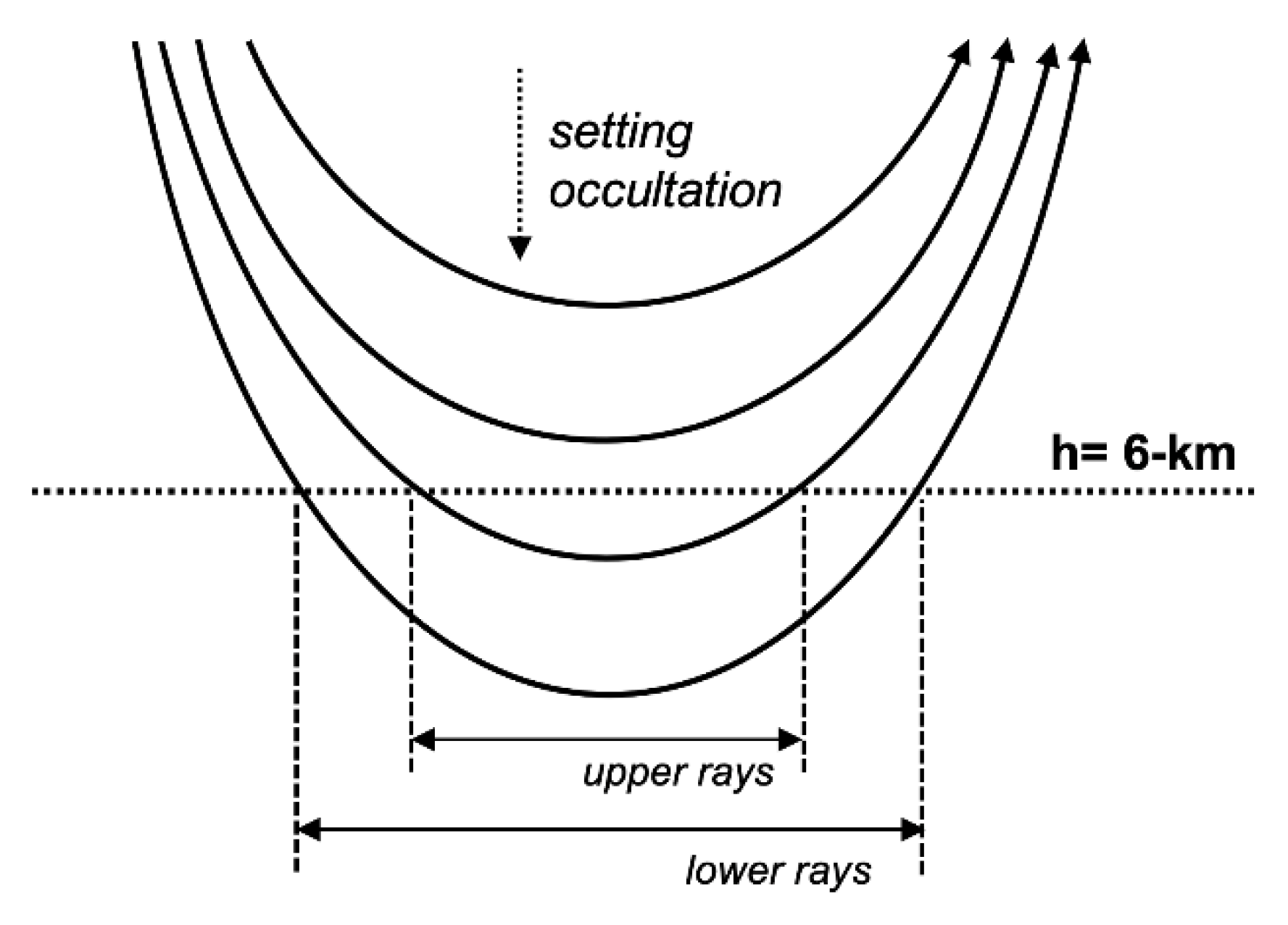
• Collections of RO observations with α closer to 90° are more perpendicular to each other, but also suffer a larger tangent point drift. In other words, even though d_eff is small in general for the 45° case, the tangent point drift will be smaller. Therefore, there is less likelihood of a ray path overlap between adjacent RO soundings.

Over one year, these event sampling numbers are sufficient for comparing convective transition statistics amongst climate models over tropical oceans, such as comparing the sharp pickup in precipitation as column water vapor exceeds a critical threshold [10], as well as sensitivity to the free-tropospheric moisture [11].

5. Conclusions

To address fundamental open questions in the cloud-convective process, a sequence of polarimetric RO measurements collected from a closely spaced LEO satellite constellation is proposed. Currently, this process lacks observational constraints, due to the difficulty in obtaining accurate, vertically resolved pressure, temperature and water vapor structure inside and near convective clouds with global coverage over land and oceans. The recent launch of the COSMIC-2 (6-satellite, 24° inclination plane) RO constellation in mid-2019 may provide RO sampling internal and external to many convective systems, but relatively few close-time events at the short time scales of moisture transport in and near convective cloud processes. From the technology aspect, the polarimetric RO concept has been proven from space with the data collected from the modified IGOR receiver (ROHP) flying onboard the Spanish PAZ satellite since early 2018. An RO receiver (Cion) suitable in size and power requirements for small 6U-sized cubesats has been successfully flown and operated.

The unique sampling offered by closely-spaced (p, q and T) profiles obtained from RO is complementary to other small satellite-based observations of the cloud structure as obtained from space-based radar, such as the RainCube Ka-band radar currently (mid-2019) being tested from space [46]. RO obtained by compact, low-power Cion-sized instruments could orbit together with small high-frequency (e.g., 183 GHz water vapor complex) passive MW sounders on the same platform, or separately in formation flying. Depending upon the orientation of the RO antenna on the receiving satellite, the RO tangent point locations can be tailored to lie outside of the MW sounder swath (effectively expanding the total coverage area), or more internal to the swath. In the latter case, the coarse along-ray but high-vertical-resolution RO data are complementary to the finer horizontal scale, but the coarse vertical-resolution-passive MW data enables the potential tomographic reconstruction of 3-D water vapor structure [47].

In addition, knowledge of the moist thermodynamic profile within heavy precipitation is useful towards the improvement and evaluation of the microphysical parameterizations used in NWP forecast models, and advancement of the state of rain-affected data assimilation [48]. The use of PRO for NWP data assimilation will require a forward observation operator that can simulate all contributions to ΔΦ along realistic RO propagation paths [37]. In addition, other applications can benefit from such a constellation (e.g., inferring horizontal wavelengths of gravity waves from multiple RO temperature profiles) [49].

References

1. Stephens, G.L.; L’Ecuyer, T.; Forbes, R.; Gettlemen, A.; Golaz, J.-C.-C.; Bodas-Salcedo, A.; Suzuki, K.; Gabriel, P.; Haynes, J. Dreary state of precipitation in global models. J. Geophys. Res. 2010, 115, D24211. [Google Scholar] [CrossRef]
2. Brown, R.G.; Zhang, C. Variability of mid-tropospheric moisture and its effect on cloud-top height distribution during TOGA COARE. J. Atmos. Sci. 1997, 54, 2760–2774. [Google Scholar] [CrossRef]
3. Holloway, C.E.; Neelin, J.D. Moisture vertical structure, column water vapor, and tropical deep convection. J. Atmos. Sci. 2009, 66, 1665–1683. [Google Scholar] [CrossRef]
4. Sherwood, S.C.; Wahrlich, R. Observed evolution of tropical deep convective events and their environment. Mon. Weather Rev. 1999, 127, 1777–1795. [Google Scholar] [CrossRef]
5. Parsons, D.B.; Redelsperger, J.-L.; Yoneyama, K. The evolution of the tropical Western Pacific atmosphere-ocean system following the arrival of a dry intrusion. Q. J. R. Meteorol. Soc. 2000, 126, 517–548. [Google Scholar] [CrossRef]
6. Tompkins, A.M. Organization of Tropical Convection in Low Vertical Wind Shears: The Role of Cold Pools. J. Atmos. Sci. 2001, 58, 1650–1672. [Google Scholar] [CrossRef]
7. Redelsperger, J.L.; Parsons, D.B.; Guichard, F. Recovery processes and factors limiting cloud-top height following the arrival of a dry intrusion observed during TOGA-COARE. J. Atmos. Sci. 2002, 59, 2438–2457. [Google Scholar] [CrossRef]
8. Derbyshire, S.H.; Beau, I.; Bechtold, P.; Grandpeix, J.Y.; Piriou, J.M.; Redelsperger, J.L.; Soares, P.M.M. Sensitivity of moist convection to environmental humidity. Q. J. R. Meteorol. Soc. 2004, 130, 3055–3079. [Google Scholar] [CrossRef]
9. Sahany, S.; Neelin, J.D.; Hales, K.; Neale, R.B. Temperature-moisture dependence of the deep convective transition as a constraint on entrainment in climate models. J. Atmos. Sci. 2012, 69, 1340–1358. [Google Scholar] [CrossRef]
10. Kuo, Y.-H.; Neelin, J.D.; Mechoso, C.R. Tropical Convective Transition Statistics and Causality in the Water Vapor-Precipitation Relation. J. Atmos. Sci. 2017, 74, 915–931. [Google Scholar] [CrossRef]
11. Schiro, K.A.; Neelin, J.D. Deep Convective Organization, Moisture Vertical Structure, and Convective Transition Using Deep-Inflow Mixing. J. Atmos. Sci. 2019, 76, 965–987. [Google Scholar] [CrossRef]
12. Haddad, Z.S.; Sawaya, R.C.; Kacimi, S.; Sy, O.O.; Turk, F.J.; Steward, J. Interpreting millimeter-wave radiances over tropical convective clouds. J. Geophys. Res. Atmos. 2017, 122, 1650–1664. [Google Scholar] [CrossRef]
13. Wentz, F.J. A 17-Yr Climate Record of Environmental Parameters Derived from the Tropical Rainfall Measuring Mission (TRMM) Microwave Imager. J. Clim. 2015, 28, 6882–6902. [Google Scholar] [CrossRef]
14. Adams, D.K.; Fernandes, R.M.; Holub, K.L.; Gutman, S.I.; Barbosa, H.M.; Machado, L.A.; Calheiros, A.J.; Bennett, R.A.; Kursinski, E.R.; Sapucci, L.F. The Amazon Dense GNSS Meteorological Network: A New Approach for Examining Water Vapor and Deep Convection Interactions in the Tropics. Bull. Am. Meteorol. Soc. 2015, 96, 2151–2165. [Google Scholar] [CrossRef]
15. Ware, R.; Rocken, C.; Solheim, F.; Feng, D.; Herman, B.; Gorbunov, M.; Businger, S. GPS sounding of the atmosphere from low earth orbit: Preliminary results. Bull. Am. Meteorol. Soc. 1996, 77, 19–40. [Google Scholar] [CrossRef]
16. Kursinski, E.R.; Hajj, G.A.; Schofield, J.T.; Linfield, R.P.; Hardy, K.R. Observing Earth’s atmosphere with radio occultation measurements using the Global Positioning System. J. Geophys. Res. Atmos. 1997, 102, 23429–23465. [Google Scholar] [CrossRef]
17. Hajj, G.A.; Kursinski, E.R.; Romans, L.J.; Bertiger, W.I.; Leroy, S.S. A technical description of atmospheric sounding by GPS occultation. J. Atmos. Sol.-Terr. Phys. 2002, 64, 451–469. [Google Scholar] [CrossRef]
18. Bauer, P.; Radnóti, G.; Healy, S.; Cardinali, C. GNSS Radio Occultation Constellation Observing System Experiments. Mon. Weather Rev. 2013, 142, 555–572. [Google Scholar] [CrossRef]
19. Cucurull, L.; Atlas, R.; Li, R.; Mueller, M.J.; Hoffman, R.N. An Observing System Simulation Experiment with a Constellation of Radio Occultation Satellites. Mon. Weather Rev. 2018, 146, 4247–4259. [Google Scholar] [CrossRef]
20. Kuo, Y.-H.; Schiro, K.A.; Neelin, J.D. Convective Transition Statistics over Tropical Oceans for Climate Model Diagnostics: Observational Baseline. J. Atmos. Sci. 2018, 75, 1553–1570. [Google Scholar] [CrossRef]
21. Padullés, R.; Cardellach, E.; Wang, K.-N.; Ao, C.O.; Turk, F.J.; Torre-Juárez, M.D.L. Assessment of global navigation satellite system (GNSS) radio occultation refractivity under heavy precipitation. Atmos. Chem. Phys. 2018, 18, 11697–11708. [Google Scholar] [CrossRef] [Green Version]
22. Biondi, R.; Randel, W.J.; Ho, S.-P.; Neubert, T.; Syndergaard, S. Thermal structure of intense convective clouds derived from GPS radio occultations. Atmos. Chem. Phys. Discuss. 2011, 11, 29093–29116. [Google Scholar] [CrossRef]
23. Murphy, M.J.; Haase, J.S.; Padullés, R.; Chen, S.-H.; Morris, M.A. The Potential for Discriminating Microphysical Processes in Numerical Weather Forecasts Using Airborne Polarimetric Radio Occultations. Remote Sens. 2019, 11, 2268. [Google Scholar] [CrossRef]
24. Bonafoni, S.; Biondi, R.; Brenot, H.; Anthes, R. Radio occultation and ground-based GNSS products for observing, understanding and predicting extreme events: A review. Atmos. Res. 2019, 230, 104624. [Google Scholar] [CrossRef]
25. Cardellach, E.; Oliveras, S.; Rius, A.; Tomás, S.; Ao, C.O.; Franklin, G.W.; Iijima, B.A.; Kuang, D.; Meehan, T.K.; Padullés, R.; et al. Sensing Heavy Precipitation with GNSS Polarimetric Radio Occultations. Geophys. Res. Lett. 2019, 46, 1024–1031. [Google Scholar] [CrossRef]
26. Skofronick-Jackson, G.; Kirschbaum, D.; Petersen, W.; Huffman, G.; Kidd, C.; Stocker, E.; Kakar, R. The Global Precipitation Measurement (GPM) mission’s scientific achievements and societal contributions: Reviewing four years of advanced rain and snow observations. Q. J. R. Meteorol. Soc. 2018, 144, 27–48. [Google Scholar] [CrossRef]
27. Huffman, G.J.; Bolvin, D.T.; Braithwaite, D.; Hsu, K.; Joyce, R.; Kidd, C.; Nelkin, E.J.; Xie, P. NASA Global Precipitation Measurement (GPM) Integrated Multi-satellitE Retrievals for GPM (IMERG); Algorithm Theoretical Basis Document, version 4.5; NASA Precipitation Measuring Missions, Goddard Space Flight Center: Greenbelt, MD, USA, 2015. Available online: http://pmm.nasa.gov/sites/default/files/document_files/IMERG_ATBD_V4.5.pdf (accessed on 11 October 2019).
28. Gorbunov, M.E.; Lauritsen, K.B. Analysis of wave fields by Fourier integral operators and their application for radio occultations. Radio Sci. 2004, 39, RS4010. [Google Scholar] [CrossRef]
29. Zeng, Z.; Sokolovskiy, S.; Schreiner, W.S.; Hunt, D. Representation of Vertical Atmospheric Structures by Radio Occultation Observations in the Upper Troposphere and Lower Stratosphere: Comparison to High-Resolution Radiosonde Profiles. J. Atmos. Ocean. Technol. 2019, 36, 655–670. [Google Scholar] [CrossRef]
30. Healy, S.B.; Eyre, J.R. Retrieving temperature, water vapour and surface pressure information from refractive-index profiles derived by radio occultation: A simulation study. Q. J. R. Meteorol. Soc. 2000, 126, 1661–1683. [Google Scholar] [CrossRef]
31. Kursinski, E.R.; Hajj, G.A. A comparison of water vapor derived from GPS occultations and global weather analyses. J. Geophys. Res. Atmos. 2001, 106, 1113–1138. [Google Scholar] [CrossRef]
32. Kursinski, E.R.; Gebhardt, T. A Method to Deconvolve Errors in GPS RO-Derived Water Vapor Histograms. J. Atmos. Ocean. Technol. 2014, 31, 2606–2628. [Google Scholar] [CrossRef]
33. Vergados, P.; Mannucci, A.J.; Ao, C.O. Assessing the performance of GPS radio occultation measurements in retrieving tropospheric humidity in cloudiness: A comparison study with radiosondes, ERA-Interim, and AIRS data sets. J. Geophys. Res. Atmos. 2014, 119, 7718–7731. [Google Scholar] [CrossRef]
34. Juárez, M.D.L.T.; Padullés, R.; Turk, F.J.; Cardellach, E. Signatures of Heavy Precipitation on the Thermodynamics of Clouds Seen from Satellite: Changes Observed in Temperature Lapse Rates and Missed by Weather Analyses. J. Geophys. Res. Atmos. 2018, 123, 13033–13045. [Google Scholar]
35. Cardellach, E.; Tomás, S.; Oliveras, S.; Padullés, R.; Rius, A.; Juárez, M.; Turk, F.J.; Ao, C.O.; Kursinki, E.R.; Schreiner, R.; et al. Sensitivity of PAZ LEO Polarimetric GNSS Radio-Occultation Experiment to Precipitation Events. IEEE Trans. Geosci. Remote Sens. 2015, 53, 190–206. [Google Scholar] [CrossRef]
36. Cardellach, E.; Padullés, R.; Tomás, S.; Turk, F.J.; Ao, C.O.; Torre-Juárez, M.D.L. Probability of intense precipitation from polarimetric GNSS radio occultation observations. Q. J. R. Meteorol. Soc. 2018, 144, 206–220. [Google Scholar] [CrossRef] [PubMed]
37. Padullés, R.; Ao, C.O.; Turk, F.J.; de la Torre-Juárez, M.; Wang, K.-N.; Iijima, B.; Cardellach, E. Calibration and Validation of the Polarimetric Radio Occultation and Heavy Precipitation experiment Aboard the PAZ Satellite. Atmos. Meas. Tech. Discuss. 2019. [Google Scholar] [CrossRef]
38. Andrić, J.; Kumjian, M.R.; Zrnić, D.S.; Straka, J.M.; Melnikov, V.M. Polarimetric Signatures above the Melting Layer in Winter Storms: An Observational and Modeling Study. J. Appl. Meteor. Climatol. 2013, 52, 682–700. [Google Scholar] [CrossRef]
39. Anthes, R.; Schreiner, W. Six new satellites watch the atmosphere over Earth’s equator. Eos 2019, 100. [Google Scholar] [CrossRef]
40. Esterhuizen, S.; Franklin, G.; Hurst, K.; Mannucci, A.; Meehan, T.; Webb, F.; Young, L. TriG—A GNSS Precise Orbit and Radio Occultation Space Receiver. In Proceedings of the 22nd International Technical Meeting of the Satellite Division of The Institute of Navigation (ION GNSS 2009), Savannah, GA, USA, 22–25 September 2009; pp. 1442–1446. [Google Scholar]
41. Franklin, G.; Esterhuizen, S.; Galley, C.; Iijima, B.; Larsen, K.; Lee, M.; Liu, J.; Meehan, T.; Young, L. A GNSS receiver for small satellites enabling precision POD, radio occultations, and reflections. In CubeSats and NanoSats for Remote Sensing II; International Society for Optics and Photonics: Bellingham, WA, USA, 2018; p. 1076905. [Google Scholar]
42. Jasper, L.; Nuding, D.; Barlow, E.; Hogan, E.; O’Keefe, S.; Withnell, P.; Yunck, T. CICERO: A Distributed Small Satellite Radio Occultation Pathfinder Mission. In Proceedings of the 27th AIAA/USU Conference, Small Satellite Constellations, Logan, UT, USA, 10–15 August 2013; Paper SSC13-IV-5. Available online: http://digitalcommons.usu.edu/cgi/viewcontent.cgi?article=2936&context=smallsat (accessed on 11 October 2019).
43. Ao, C.O.; Hajj, G.A.; Meehan, T.K.; Dong, D.; Iijima, B.A.; Mannucci, A.J.; Kursinski, E.R. Rising and setting GPS occultations by use of open-loop tracking. J. Geophys. Res. Atmos. 2009, 114, D04101. [Google Scholar] [CrossRef]
44. Bringi, V.N.; Chandrasekar, V. Polarimetric Weather Radar: Principles and Applications; Cambridge University Press: New York, NY, USA, 2001. [Google Scholar]
45. Foelsche, U.; Syndergaard, S.; Fritzer, J.; Kirchengast, G. Errors in GNSS radio occultation data: Relevance of the measurement geometry and obliquity of profiles. Atmos. Meas. Tech. 2011, 4, 189–199. [Google Scholar] [CrossRef]
46. Peral, E.; Im, E.; Wye, L.; Lee, S.; Tanelli, S.; Rahmat-Samii, Y.; Horst, S.; Hoffman, J.; Yun, S.; Imken, T.; et al. Radar Technologies for Earth Remote Sensing from CubeSat Platforms. Proc. IEEE 2018, 106, 404–418. [Google Scholar] [CrossRef]
47. Möller, G.; Landskron, D. Atmospheric bending effects in GNSS tomography. Atmos. Meas. Tech. 2019, 12, 23–34. [Google Scholar] [CrossRef] [Green Version]
48. Geer, A.J.; Baordo, F.; Bormann, N.; Chambon, P.; English, S.J.; Kazumori, M.; Lawrence, H.; Lean, P.; Lonitz, K.; Lupu, C. The growing impact of satellite observations sensitive to humidity, cloud and precipitation. Q. J. R. Meteorol. Soc. 2017, 143, 3189–3206. [Google Scholar] [CrossRef]
49. Faber, A.; Llamedo, P.; Schmidt, T.; De La Torre, A.; Wickert, J. On the determination of gravity wave momentum flux from GPS radio occultation data. Atmos. Meas. Tech. 2013, 6, 3169–3180. [Google Scholar] [CrossRef] [Green Version]
Figure 1. A graphical depiction of the closely spaced radio occultation (RO) observation strategy. In this depiction, three polarimetric RO-receiving capable satellites orbit in formation with a time separation near two minutes. The short time separation increases the likelihood that all three satellites observe the same occulting GNSS satellite, and one or more ray path profiles transects through the atmosphere containing a region of heavy precipitation (dark grey) and the nearby environment outside of heavy precipitation (light grey).
Remotesensing 11 02399 g001
Figure 2. A depiction of the polarimetric RO measurement concept. As the right-hand circularly (RHC) polarized transmitted GNSS signal propagates through a region of heavy precipitation characterized by aspherical hydrometeors, an orthogonal (i.e., cross-polarized) left-hand circularly (LHC) polarized component is induced. The co- and cross-polarized signals are measured by a GNSS receiver at two linear (horizontal and vertical, denoted H and V) orthogonal polarizations.
Remotesensing 11 02399 g002
Figure 3. ROHP observations on May 23, 2018 in the presence of tropical cyclone Mekunu (Category 3). The tangent point location and ray orientation of five ROHP observations are represented by the circle symbol and the thick blue line. The five insets, corresponding to each Radio Occultations through Heavy Precipitation (ROHP) observation, show the measured H-V differential phase shift in mm as a function of height (green), alongside the profile of temperature (orange) and water vapor partial pressure (blue) obtained from PAZ at the same time. Large polarimetric phase differences were obtained up to a 10 km height from the ROHP observations in regions associated with heavy precipitation surrounding the eyewall near 55E/10N. Regions of no precipitation near 40E/3S show no significant signal. The background color represents the observed geostationary satellite infrared brightness temperature (Kelvin), which is shown as a proxy for cloud top height and associated convective precipitation intensity.
Remotesensing 11 02399 g003
Figure 4. The geographical distribution of the upper percentile (top 2%) of the measured Δ ϕ   from all ROHP observations between 60S and 60N latitudes. Each color denotes a vertical region where the Δ ϕ from all rays were averaged. Black, orange and red symbols represent cases where the average Δ ϕ   was obtained by averaging all RO rays whose tangent point lies between 0–5, 5–10 and 10–15 km height, respectively. The top panel includes all data for June–July–August (JJA); the lower panel for December–January–February (DJF). The color background map depicts the average rain rate during these months derived from the GPM IMERG precipitation product.
Remotesensing 11 02399 g004
Figure 5. A picture of the Cion RO receiver instrument flying onboard the CICERO 6U-sized cubesats (right), shown alongside the size of the larger TriG receiver (left) flying onboard each of the six satellites in the COSMIC-2 constellation.
Remotesensing 11 02399 g005
Figure 6. The location of the RO tangent points for the events where the intersected precipitation induced a propagation cumulative differential phase shift (ΔΦ) >6 mm. The different colors indicate each low earth-orbiting (LEO) satellite, where LEO = 1 (blue) and LEO = 3 (green) are the leading and trailing satellite in the constellation, respectively.
Remotesensing 11 02399 g006
Figure 7. (a) Histogram of the distance (km) between the tangent point locations of the RO acquired with the first and second satellite of the train constellation (blue), and with the first and third satellites (orange). (b) Same as left panel, but for the time difference (seconds) between the RO tangent point locations.
Remotesensing 11 02399 g007
Figure 8. A simulated three-satellite RO orbit scenario, superimposed upon nearest 30 min IMERG precipitation pattern. (a) Representation of an event where two of the RO observations (RO-1 and RO-2; green and orange, respectively) provide profiles that intersect precipitation, while a third (RO-3; blue) profiles the environment outside of the precipitating structure. The colored rays represent a realistic representation of RO rays generated with a ray-tracer and are positioned here for illustration purposes. Only the portion of the rays below 6 km is shown. For each RO, the associated “X” symbol depicts the location of the tangent point. The black dashed line shows a single simplified 300 km ray used to characterize each RO. (b) The same RO event as (a), depicting the difference that the relative angle (α) between the azimuth on the surface and the along-track occultations has from the geometry of the observations. In this event, the angle is almost 90°, with an across-RO separation (denoted by d) of about 100 km. (c) The same as (b), but a different RO event where the relative angle (α) is around 10°. The effective distance deff between the rays is reduced to near 20 km, even though the separation between the tangent points d remain nearly the same as event (b).
Remotesensing 11 02399 g008
Figure 9. A depiction of the horizontal extent of the rays corresponding to RO ray paths whose bending falls below a fixed height (shown here at 6 km). The lower rays project a longer horizontal distance relative to upper rays.
Remotesensing 11 02399 g009
Figure 10. (a) A 2-dimensional (2-D) histogram of the relative angle (α) between the along-ray direction and the line joining the tangent points, as a function of the associated tangent point separation difference d (see Figure 8). Only those RO events that had at least one observation that detected precipitation (i.e., ΔΦ > 1.5 mm, denoted as “inside precipitation”) and at least one observation that did not detect precipitation (i.e., ΔΦ < 1.5 mm, denoted as “outside precipitation”) are considered. (b) An associated 1-D histogram of the tangent point separation difference d. (c) An associated 1-D histogram of the distribution of angles between the along-ray direction and the line joining the tangent points.
Remotesensing 11 02399 g010
Figure 11. A summary of the distribution of distances for the cases with inside and outside precipitation observations (gray box histogram), and the effective distances deff between rays accounting for the angle α (blue line histogram) for the different orbit configurations. (Left panels) The results for a 45° orbit inclination. (Right panels) The results for a 98° orbit inclination. In each of the left and right sides, from top to bottom, the results are shown for the number and positions of RO-capable receiving satellites indicated in Table 1. The labels embedded within each panel provide the absolute numbers corresponding to each histogram, and the ratio between the cases with deff > 25 km with respect to the total cases (green font).
Remotesensing 11 02399 g011