Article

Spatial-Spectral Multiple Manifold Discriminant Analysis for Dimensionality Reduction of Hyperspectral Imagery

Key Laboratory on Opto-Electronic Technique and Systems, Ministry of Education, Chongqing University, Chongqing 400044, China
*
Author to whom correspondence should be addressed.
Remote Sens. 2019, 11(20), 2414; https://0-doi-org.brum.beds.ac.uk/10.3390/rs11202414
Submission received: 14 September 2019 / Revised: 13 October 2019 / Accepted: 15 October 2019 / Published: 18 October 2019
(This article belongs to the Special Issue Advanced Techniques for Spaceborne Hyperspectral Remote Sensing)

Abstract

:
Hyperspectral images (HSI) possess abundant spectral bands and rich spatial information, which can be utilized to discriminate different types of land cover. However, the high dimensional characteristics of spatial-spectral information commonly cause the Hughes phenomena. Traditional feature learning methods can reduce the dimensionality of HSI data and preserve the useful intrinsic information but they ignore the multi-manifold structure in hyperspectral image. In this paper, a novel dimensionality reduction (DR) method called spatial-spectral multiple manifold discriminant analysis (SSMMDA) was proposed for HSI classification. At first, several subsets are obtained from HSI data according to the prior label information. Then, a spectral-domain intramanifold graph is constructed for each submanifold to preserve the local neighborhood structure, a spatial-domain intramanifold scatter matrix and a spatial-domain intermanifold scatter matrix are constructed for each sub-manifold to characterize the within-manifold compactness and the between-manifold separability, respectively. Finally, a spatial-spectral combined objective function is designed for each submanifold to obtain an optimal projection and the discriminative features on different submanifolds are fused to improve the classification performance of HSI data. SSMMDA can explore spatial-spectral combined information and reveal the intrinsic multi-manifold structure in HSI. Experiments on three public HSI data sets demonstrate that the proposed SSMMDA method can achieve better classification accuracies in comparison with many state-of-the-art methods.

Graphical Abstract

1. Introduction

Hyperspectral image (HSI) is acquired by different imaging spectrometer sensors (e.g., EO-1 Hyperion, HyMap and AVIRIS), which possesses abundant spectral information about ground objects in hundreds of spectral bands [1,2,3]. Due to the advancement of imaging spectrometer technology, the spectral resolution of hyperspectral sensors has been improved significantly, which can provide richer spectral information to differentiate different ground objects [4,5]. However, the sensors with higher resolution produce a very large volume of data, it will render the traditional image processing algorithms designed for multispectral imagery ineffective [6,7]. In particular, the high dimensionality of HSI data brings about the “curse of dimensionality” problem, that is, under a fixed, small number of training samples, the classification accuracy of HSI data decreases when the dimensionality of HSI data increases [8,9,10]. Besides, the spectral bands are highly correlated and some spectral bands may not carry discriminant information in a specific application. The reason is that the sample point in HSI often exhibits similar characteristics to electromagnetic waves in adjacent bands, which will produce a lot of useless information and restrict the classification performance of HSI. Therefore, to achieve an excellent classification performance, it is an urgent task to perform dimensionality reduction (DR) for HSI data while preserving the intrinsic valuable information.
Serving as a good tool for data mining, manifold learning has been the main focus of DR [11,12,13]. Recently, many manifold learning algorithms have been introduced to discover the intrinsic structure in high-dimensional data, such methods include local linear embedding (LLE) [14], Laplacian eigenmaps (LE) [15] and isometric feature mapping (ISOMAP) [16]. LLE assumes that the data is linear over a small locality, it preserves the local linear structure of data in low-dimensional space [17]. LE builds a graph incorporating neighborhood information of data and computes a low-dimensional representation by optimally preserving local neighborhood information [18]. ISOMAP characterizes the data distribution by geodesic distances instead of Euclidean distances, it seeks a lower-dimensional embedding which maintains geodesic distances between all points [19]. However, due to their nonlinear characteristic, they suffer from the problem of out-of-sample and cannot process the unknown samples [20,21,22]. To address this issue, many linear manifold learning methods were designed to obtain explicit feature mappings, which can map unknown samples into low-dimensional space [23,24]. The representative methods include neighborhood preserving embedding (NPE) [25], locality preserving projection (LPP) [26] and local scaling cut (LSC) [27]. NPE aims at preserving the local manifold structure which is constructed by the k-nearest neighbors [28]. LPP seeks an optimal linear projection while preserving the local geometry structure in original data [29]. LSC uses the spectral information to explore the intrinsic manifold structure of HSI data by constructing a pairwise dissimilarity matrix [30]. Although the motivations of the methods are different, their common objective is to derive a lower-dimensional representation and facilitate the subsequent classification task. In order to unify these methods, a graph embedding (GE) framework was proposed to describe many existing DR techniques [31]. Based on this framework, local geometric structure Fisher analysis(LGSFA) was proposed by compacting the homogeneous data while separating the heterogeneous data [32]. However, the above manifold learning methods assume that the observed data is located on a single manifold and they cannot discover the multi-manifold structure embedded in HSI. Therefore, the single manifold methods have a limited discriminating power to distinguish different land covers and their classification performance will be reduced rapidly when applied to more complex scenes.
In practical applications, the observed data can be divided into many different subsets and each subset resides on a low-dimensional submanifold [33]. To reveal the multi-manifold structure in high-dimensional data, some multiple manifold learning methods were explored for feature learning. Hettiarachchi et al. [34] proposed a multiple manifold locally linear embedding (MM-LLE) algorithm which adopts a supervised LLE form of neighborhood selection in learning individual manifolds and it uses a manifold-manifold distance (MMD) as a measure to find the optimum embedded dimension. Jiang et al. [35] proposed a coupled discriminant multi-manifold analysis (CDMMA) algorithm which explores the neighborhood information as well as local geometric structure of the multi-manifold space spanned by samples and it exploits the discriminant information by minimizing the intramanifold distance and maximizing the intermanifold distance simultaneously. Chu et al. [36] proposed a multi-feature multi-manifold learning (M 3 L) method, which learns multiple discriminative feature subspaces by maximizing the multi-feature manifold margins of different classes and it recognizes the probe subjects with a multi-feature manifold-manifold distance. Shi et al. [37] proposed a supervised multi-manifold learning (SMML) algorithm, which extracts multi-manifold features through maximizing the between-class Laplacian graph and projects samples from different classes into respective submanifolds. Although the multiple manifold learning methods can enhance the classification performance of high-dimensional data, they ignore the spatial consistency property of HSI and do not utilize the abundant spatial information.
Spatial information has been proven to be useful for improving the classification performance of HSI [38,39]. Recently, many DR methods have been proposed based on the spatial distribution of hyperspectral data and they can be divided into two main types: spatial filtering methods and spatial DR methods [40,41,42]. Spatial filtering methods focus on how to utilize spatial homogeneous regions to smooth the pixel-wise classification map, while spatial DR methods incorporate spatial information into the process of DR by modeling the spatial neighboring correlations [43,44]. Although spatial filtering techniques can improve the classification accuracy of HSI data, they are often used as the pre-processing techniques to process the whole image [45]. In view of this, spatial DR methods have been widely studied for HSI classification [46,47]. Zhou et al. [48] proposed a spatial-domain local pixel NPE (LPNPE) method, which seeks a linear projection by minimizing the local pixel neighborhood preserving scatter and maximizing the total scatter of data. Feng et al. [49] developed a discriminate spectral-spatial margins (DSSM) method, which reveals the local neighborhood information of HSI data and explores the global structure of labeled and unlabeled data via low rank representation. Ramanarayan et al. [50] designed a neighboring pixel local scaling cut (NPLSC) method, which combines the unlabeled spectral weight with the local graph cut-based segmentation strategy on the homogeneous HSI data to maintain the label consistency in the spatial domain. The spatial-spectral combined DR methods have improved the classification performance significantly but they do not consider the multi-manifold structure of HSI data to further enhance the classification performance.
To explore the multiple manifold structure and spatial information in HSI, we proposed a novel spatial-spectral multi-manifold DR method, called spatial-spectral multiple manifold discriminant analysis (SSMMDA) for HSI classification. Differently from the methods of spatial filtering, SSMMDA incorporates spatial information into the DR process for feature learning. The main contributions of SSMMDA can be summarized as following. (1) According to the prior label information of training samples, we divide the samples data into several different subsets, each subset is treated as a submanifold. (2) Based on the graph embedding theory, an intramanifold graph is constructed for each submanifold to preserve the local neighborhood structure in spectral domain and an intramanifold scatter matrix and an intermanifold scatter matrix are constructed for each submanifold to characterize the within-manifold compactness and the between-manifold separability in spatial domain. (3) A spatial-spectral combined objective function is designed for each submanifold and each submanifold can obtain a discriminant projection matrix by maximizing the spatial-spectral intermanifold scatter matrix and minimizing the spatial-spectral intramanifold scatter matrix simultaneously. (4) Embedding features for each submanifold can be obtained via the corresponding projection matrix and then different embedding features are fused to enhance the classification performance.
The remainder of the paper is structured as follows. Section II briefly reviews some related works including GE and LSC. Section III details our proposed SSMMDA method. Section IV reports the experimental results. Section V presents some analysis and discussion on the experiments. Finally, Section VI provides our concluding remarks and gives recommendations for future work.

2. Related Works

Suppose that a HSI data set X contains n samples with D bands, i-th pixel can be represented as x i R D . Denote the class label of x i as l i { 1 , 2 , , c } , where c is the number of land-cover types. For linear manifold learning methods, the goal is to seek a projection matrix V R D × d , which can map X R D × n into a d-dimension embedding space, where dD. With the projection matrix V , we can compute low-dimensional embedding features Y R d × n as Y = V T X .

2.1. Graph Embedding

The graph embedding (GE) framework embeds a graph into a vector space where the inherent properties of the graph can be preserved. In GE, an intrinsic graph G = { X , W } and a penalty graph G P = X , W P are constructed based on the statistical or geometric properties of data, where X is the vertex set, W R n × n and W P R n × n are the similarity matrices of G and G P , respectively. Intrinsic graph G is used to describe desirable statistical or geometrical properties of data, while penalty graph G P is adopted to characterize dissimilarity relationship between the vertex pairs.
The purpose of GE is to represent each sample as a low-dimensional vector in graphs which can preserve similarity relationship of vertex pairs. The optimal low-dimensional embedding can be given by the graph preserving criterion as Equation (1):
min tr Y T B Y = h 1 2 i j y i y j 2 w i j = min tr Y T B Y = h tr Y T L Y
where h is a constant, B is a constraint matrix which is defined to avoid the trivial solution of Equation (1). For scale normalization, B is typically set as a diagonal matrix or the Laplacian matrix of G P . Then, the Laplacian matrices L and L P in graphs G and G P can be defined as Equations (2) and (3):
L = D W , D = diag j = 1 n w 1 j , j = 1 n w 2 j , , j = 1 n w n j , W = w i j i , j = 1 n
L P = D P W P , D P = diag j = 1 n w 1 j P , j = 1 n w 2 j P , , j = 1 n w n j P , W P = w i j P i , j = 1 n

2.2. Local Scaling Cut

Local scaling cut (LSC) is proposed based on GE framework, it compacts the data which come from the same class and separates the data which come from different classes. LSC seeks a linear projection matrix such that the between-class dissimilarity matrix is maximized, whereas the total-class dissimilarity matrix is minimized in the projected space.
To exploit the intrinsic geometry and local manifold structure of the data, LSC constructs a localized k-nearest neighbor graph to characterize the similarity relationship between the neighboring pixels. Suppose N b x i represents the k b -nearest neighbors of x i from different classes and  N w x i represents the k w -nearest neighbors of x i from the same class, then the local between-class dissimilarity matrix S b and the local within-class dissimilarity matrix S w can be given in Equations (4) and (5) as:
S b = s = 1 c x i U s x j N b x i H i j b x i x j x i x j T
S w = s = 1 c x i U s x j N w x i H i j w x i x j x i x j T
where U s denotes all the samples in s-th class, H i j b and H i j w are the weights of x i and x j in N b x i and N w x i , respectively. The weights H i j b and H i j w are defined in Equations (6) and (7) as:
H i j b = 1 / ( n s k b ) x j N b x i 0 otherwise
H i j w = 1 / ( n s k w ) x j N w x i 0 otherwise
in which n s is the total number of elements in the s-th class. Then the local scaling cut criterion is formulated as Equation (8):
S c u t s ( V ) = max V tr V T S b V tr V T S b + S w V = max V tr V T S b V tr V T T V

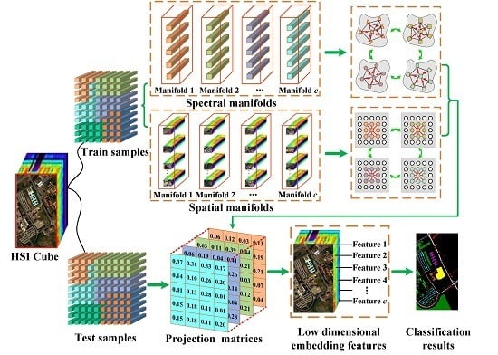
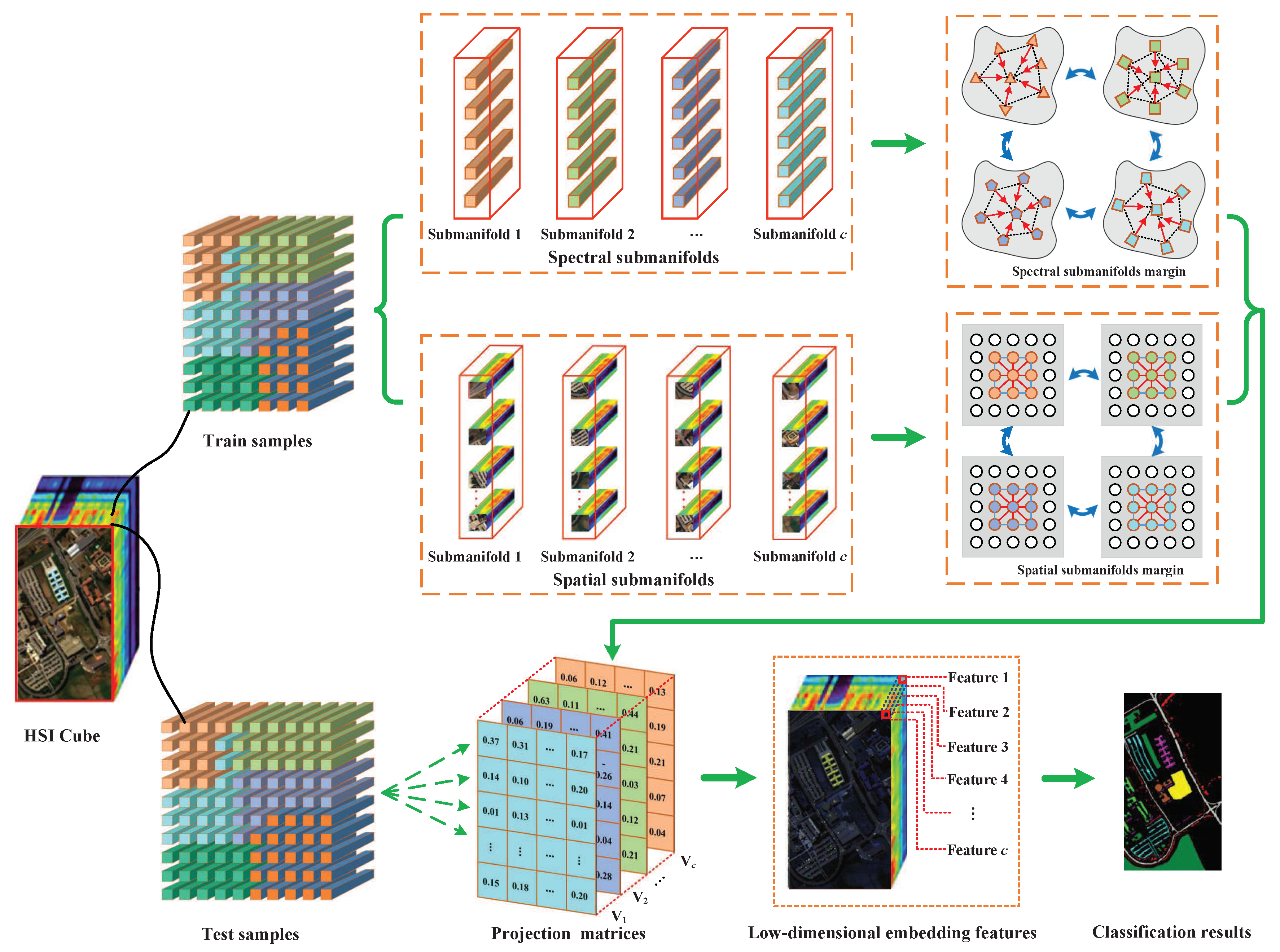
3. Spatial-Spectral Multi-Manifold Discriminant Analysis

To effectively reveal the intrinsic multi-manifold structure of HSI data, a spatial-spectral multi-manifold discriminant analysis (SSMMDA) method was proposed for DR. SSMMDA divides samples into different subsets based on their label information, each subset is treated as a submanifold. Then, for each submanifold, it selects spectral neighbors to construct a spectral-domain intramanifold graph to preserve the local neighborhood structure of HSI and it constructs two weighted scatter matrices in spatial domain to characterize the within-manifold compactness and the between-manifold separability. After that, a spatial-spectral combined objective function is designed for each submanifold and we can seek a discriminant projection matrix for each submanifold by maximizing the spatial-spectral intermanifold scatter matrix and minimizing the spatial-spectral intramanifold scatter matrix simultaneously. Finally, low-dimensional embedding for each submanifold can be obtained by corresponding projection matrix and embedding features of each submanifold are fused for classification. SSMMDA improves both the intramanifold compactness and intermanifold separability of HSI data, it possesses a better discriminative power to improve classification performance. The process of the SSMMDA method is shown in Figure 1.

3.1. Spectral-Domain Multi-Manifold Analysis Model

In some situations, high-dimensional data do not lies on a single manifold, samples from different classes lie on different submanifolds [33,34]. Existing manifold learning algorithms usually characterize the similarity relationships of high-dimensional data in the same manifold space and they can not discover the multi-manifold structure of data. Therefore, it is a crucial issue to preserve the local structure of different submanifolds by performing multiple manifold learning. In the proposed SSMMDA method, a multi-manifold learning model in spectral domain is designed to reveal the multi-manifold structure of HSI. At first, according to the label information of training samples, HSI data is divided into different subsets. Then, several intramanifold graphs are constructed in spectral domain for different subsets, which can effectively characterize the similarity relationship between samples belonging to the same submanifold.
For HSI data, each class can be treated as a submanifold. Therefore, a HSI data set with D bands can be represented as X = M 1 , M 2 , , M c R D × c , where c is the number of land-cover types. Denote the i-th point in the r-th submanifold as M r i , then the r-th submanifold can be given as M r = M r 1 , M r 2 , M r 3 , , M r n r , where n r is the number of samples in M r .
To characterize the discriminative manifold structure of M r , a spectral domain intramanifold graph G r M r , W r can be constructed, where M r is the vertex set of the graph and W r is the weight matrix. In graph G r , an edge is put between nodes i and j if M r i and M r j are neighbors, otherwise they will not be connected and the weight between M r i and M r j can be defined as Equation (9):
w r i j = exp M r i M r j 2 2 t r i 2 , M r j N i k M r i or M r i N j k M r j 0 , otherwise
where N i k M r i is the neighbor set of M r i , k is the number of intramanifold neighbors for graph G r and t r i = 1 k j = 1 k M r i M r j is a heat kernel parameter.
To enhance the aggregation of data points which possess similar spectral characteristics in low-dimensional space, the objective function can be given in Equation (10):
min V 1 , V 2 , , V c J V 1 , V 2 , , V c = min V 1 , V 2 , , V c ψ V 1 + ψ V 2 + + ψ V c = min V 1 , V 2 , , V c [ 1 2 i = 1 n 1 j = 1 k y 1 i y 1 j 2 w 1 i j + 1 2 i = 1 n 2 j = 1 k y 2 i y 2 j 2 w 2 i j + , , + 1 2 j = 1 n c j = 1 k y c i y c j 2 w c i j ] = r = 1 c min V r ( 1 2 i = 1 n r j = 1 k y r i y r j 2 w r i j )
in which y r i and y r j are the low-dimensional representations of M r i and M r j for submanifold M r , respectively.
According to Equation (10), c different projection matrices can be obtained. For the r-th submanifold in spectral domain, the optimization problem of submanifold M r can be transformed as Equation (11):
min V r ( 1 2 i = 1 n r j = 1 k y r i y r j 2 w r i j ) = min V r ( 1 2 i = 1 n r j = 1 k V r T M r i V r T M r j 2 w r i j ) = min V r ( tr ( V r T 1 2 i = 1 n r j = 1 k M r i w r i j M r i T 2 M r i w r i j M r j T + M r j w r i j M r j T V r ) ) = min V r ( tr ( V r T M r D r W r M r T V r ) ) = min V r ( tr ( V r T M r B r M r T V r ) )
where the affinity matrix W r is used to generate the intramanifold graph Laplacian matrix B r = D r W r and D r is a diagonal matrix whose entries are column sums of W r .
To eliminate the impact of scale factor, a constraint Y r D r Y r T = V r T M r D r M r T V r = I is added for Equation (11), where I = diag [ 1 , , 1 ] . Therefore, the optimal function of Equation (11) equals to the following optimization problem of Equation (12):
min V r V r T M r B r M r T V r s.t. V r T M r D r M r T V r = I
With the Lagrange multiplier method, the optimization problem in Equation (12) can be transformed into the following generalized eigenvalue problem of Equation (13):
M r B r M r T V r = λ r M r D r M r T V r
where λ r is the eigenvalue.

3.2. Spatial-Domain Multi-Manifold Analysis Model

According to the spatial distribution consistency of HSI, the pixels are generally distributed in blocks, such as Soil, Water, Building and Woods [51]. Therefore, the neighboring pixels in a spatial window are more likely belonging to the same class and they lie on the same manifold [52]. To utilize the spatial information in HSI, a spatial-domain weighted intramanifold scatter matrix is designed to characterize the similarity relationship for each submanifold and a spatial-domain weighted intermanifold scatter matrix is defined to represent the dissimilarity relationship between different submanifolds.
Suppose a pixel x i in HSI lies on the r-th spectral submanifold, then it can be represented as M r i . Since the pixels in the local spatial patch of x i commonly lie on the same submanifold as x i , so the neighboring pixels can be given as M r i 1 , M r i 2 , M r i 3 , …, M r i w 2 , where the odd number w is the size of spatial window.
From the viewpoint of classification, we aim to minimize the distances of intramanifold points and maximize the distances between different submanifolds in low-dimensional space so that the submanifold margins can be maximized for DR. Denoting y r i and y r i j as the low-dimensional representations of i-th sample and its j-th spatial neighbor in the r-th manifold space, the optimization problem can be formulated as Equation (14):
min V 1 , V 2 , , V c J V 1 , V 2 , , V c = min V 1 , V 2 , , V c ψ V 1 + ψ V 2 + + ψ V c = min V 1 , V 2 , , V c i = 1 n 1 j = 1 w 2 y 1 i y 1 i j 2 s 1 i j i = 1 n y i 1 y ¯ 1 2 s 1 i + i = 1 n 2 j = 1 w 2 y 2 i y 2 i j 2 s 2 i j i = 1 n y i 2 y ¯ 2 2 s 2 i + , , + i = 1 n c j = 1 w 2 y c i y c i j 2 s c i j i = 1 n y i c y ¯ c 2 s c i = r = 1 c min V r i = 1 n r j = 1 w 2 y r i y r i j 2 s r i j i = 1 n y i r y ¯ r 2 s r i
where y i r is the low-dimensional representation of i-th sample in the r-th manifold space, y ¯ r is the mean of all training data after they are mapped to submanifold M r , s r i j = exp y r i y r i j 2 / 2 ( t i j ) 2 is the similarity weight between y r i and y r i j , s r i = exp y i r y ¯ r 2 / 2 ( t i j ) 2 is the similarity weight between y i r and y ¯ r and t i j = 1 k j = 1 k y r i y r i j is a heat kernel parameter.
Considering that the c projection matrices are independent of each other, we can divide Equation (14) into different parts and solve them separately. As for the submanifold M r , the optimization problem can be written as Equation (15):
min V r i = 1 n r j = 1 w 2 y r i y r i j 2 s r i j i = 1 n y i r y ¯ r 2 s r i = min V r tr i = 1 n r t = 1 w 2 V r M r i V r M r i j 2 s r i j i = 1 n V r M r i V r M ¯ 2 s r i = min V r tr V r T i = 1 n r j = 1 w 2 M r i M r i j 2 s r i j V r V r T i = 1 n V r M r i V r M ¯ 2 s r i V r = min V r tr V r T H r V r V r T S r V r
in which M ¯ is the mean of all samples in HSI data, H r and S r are the intramanifold scatter matrix and the intermanifold scatter matrix for the submanifold M r and they can be defined as Equations (16) and (17):
H r = i = 1 n r j = 1 w 2 M r i M r i j 2 s r i j = i = 1 n r j = 1 w 2 M r i M r i j M r i M r i j T s r i j
S r = i = 1 n M r i M ¯ 2 s r i
After that, an optimal projection matrix V r = v r 1 , v r 2 , , v r d can be obtained by solving the generalized eigenvalue problem of Equations (18):
H r V r = λ r S r V r
in which λ r is the eigenvalue of Equation (18).

3.3. Spatial-Spectral Multi-Manifold Analysis Model

In HSI, spectral information and spatial structure are complementary to each other, spectral information characterizes the spectrum reflection characteristics of land covers, while spatial information reflects the spatial relationship of objects. To learn discriminant projections, the spectral and spatial information can be combined for feature learning. Therefore, we propose a spatial-spectral multiple manifold-based DR method for HSI classification, which extracts the feature information of HSI from both spatial and spectral domains and it can effectively reveal the multi-manifold structure in HSI.
By combining the spatial information and spectral information, we can obtain a spatial-spectral intramanifold scatter matrix and a spatial-spectral intermanifold scatter matrix for submanifold M r as Equations (19) and (20):
Z r i n t r a = M r B r M r T + α H r
Z r i n t e r = M r D r M r T + β S r
in which α and β are the tradeoff parameters which are used to balance the contribution of spatial and spectral information in the process of DR.
With the Lagrange multiplier method, the optimization problem for submanifold M r can be transformed into the following form of Equation (21):
( M r B r M r T + α H r ) V r = λ r ( M r D r M r T + β S r ) V r
in which λ r is the eigenvalue of Equation (21). After obtaining the eigenvectors v r 1 , v r 2 , v r 3 , , v r d corresponding to the d smallest eigenvalues, the optimal projection matrix can be given by Equation (22):
V r = v r 1 , v r 2 , , v r d D × d
With the same operations, different projection matrices V 1 , V 2 , , V c can be obtained as Equation (22), which correspond to different submanifolds embedded in HSI data. Denote the feature representations of X in each low-dimensional space as Y 1 = V 1 T X , Y 2 = V 2 T X , , Y c = V c T X , then the embedding features can be fused to enhance the classification performance of HSI and the fused features of X are expressed as Y = Y 1 , Y 2 , , Y c . The detailed steps of SSMMDA are shown in Algorithm 1.
Algorithm 1 SSMMDA
Input: 
HSI data set X = x 1 , x 2 , x 3 , , x n and the class label l i { 1 , 2 , 3 , , c } , spatial window size w, neighbor number k, tradeoff parameters α and β and embedding dimension d (dD).
1:
Divide the HSI data into c different submanifolds of M 1 , M 2 , M 3 , …, M c ,
2:
for r = 1 to c do
3:
     Find the spectral-domain intramanifold neighbors set N i k M r i of M r i .
4:
     Calculate intramanifold graph weight by Equation (9).
5:
     Compute intramanifold graph scatter matrix M r B r M r T and constraint matrix M r D r M r T .
6:
     Find the spatial-domain neighboring pixels set of M r i .
7:
     Compute the intramanifold scatter matrix H r and the intermanifold scatter matrix S r in spatial domain.
8:
  Compute the spatial-spectral intramanifold scatter matrix Z r intra and the spatial-spectral intermanifold scatter matrix Z r inter .
9:
     Solve the generalized eigenvalue problem of Equation (21).
10:
     Obtain the projection matrix V r for submanifold M r : V r = v r 1 v r 2 v r d R D × d
11:
end for
12:
Obtain c different projection matrices as V 1 , V 2 , , V c .
13:
Calculate the low dimensional features of X in each submanifold as Y 1 , Y 2 , …, Y c , where Y 1 = V 1 T X , Y 2 = V 2 T X , …, Y c = V c T X
Output: 
The low-dimensional features are represented as Y = Y 1 , Y 2 , , Y c

4. Experimental Results

In this section, three public HSI data sets are adopted to evaluate the effectiveness of SSMMDA by comparing it with some state-of-art DR algorithms. Experiments on these HSI data sets demonstrate that the proposed SSMMDA method can explore spatial-spectral combined information and reveal the intrinsic multi-manifold structure in HSI, which can significantly improve the classification performance of HSI.

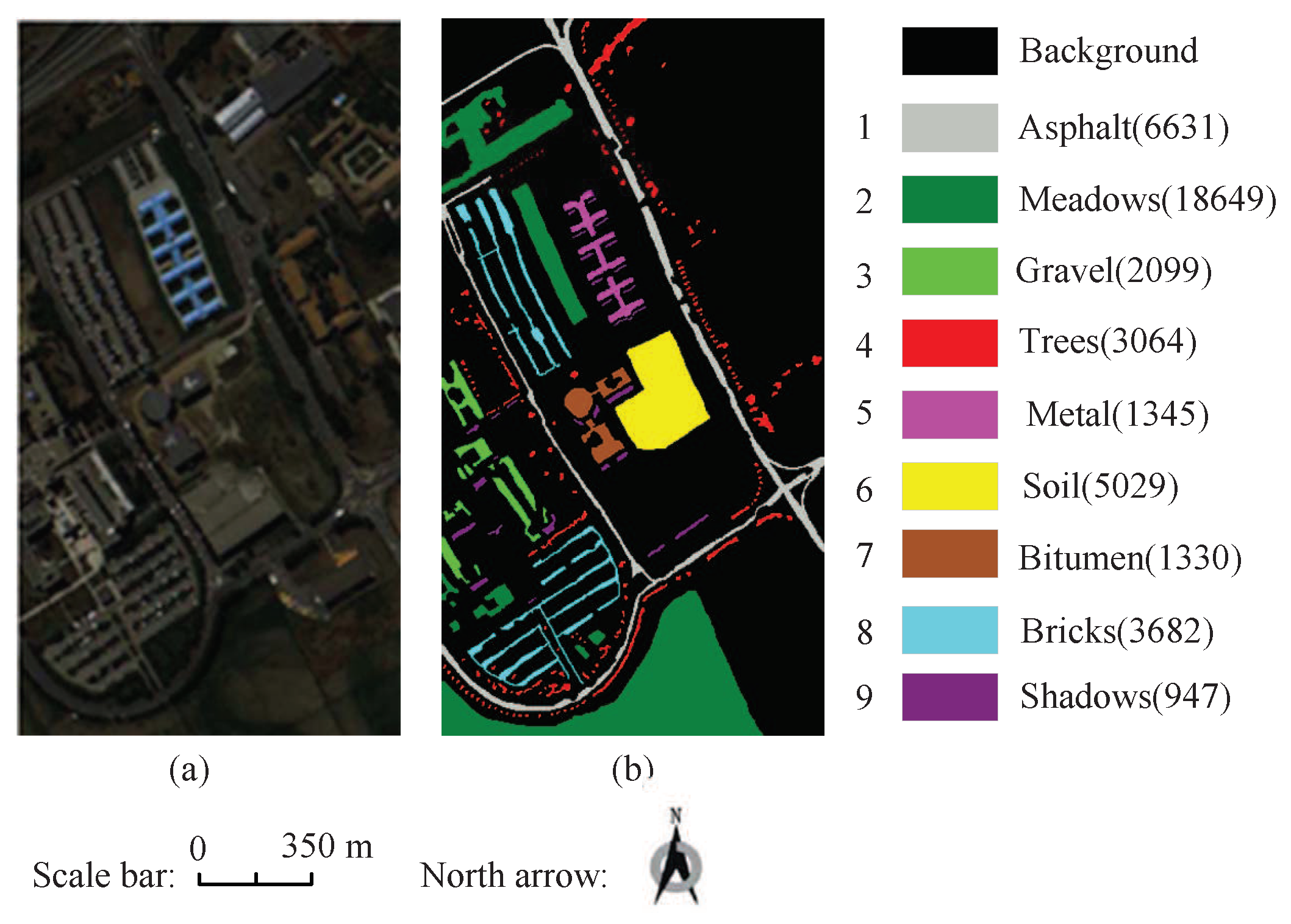
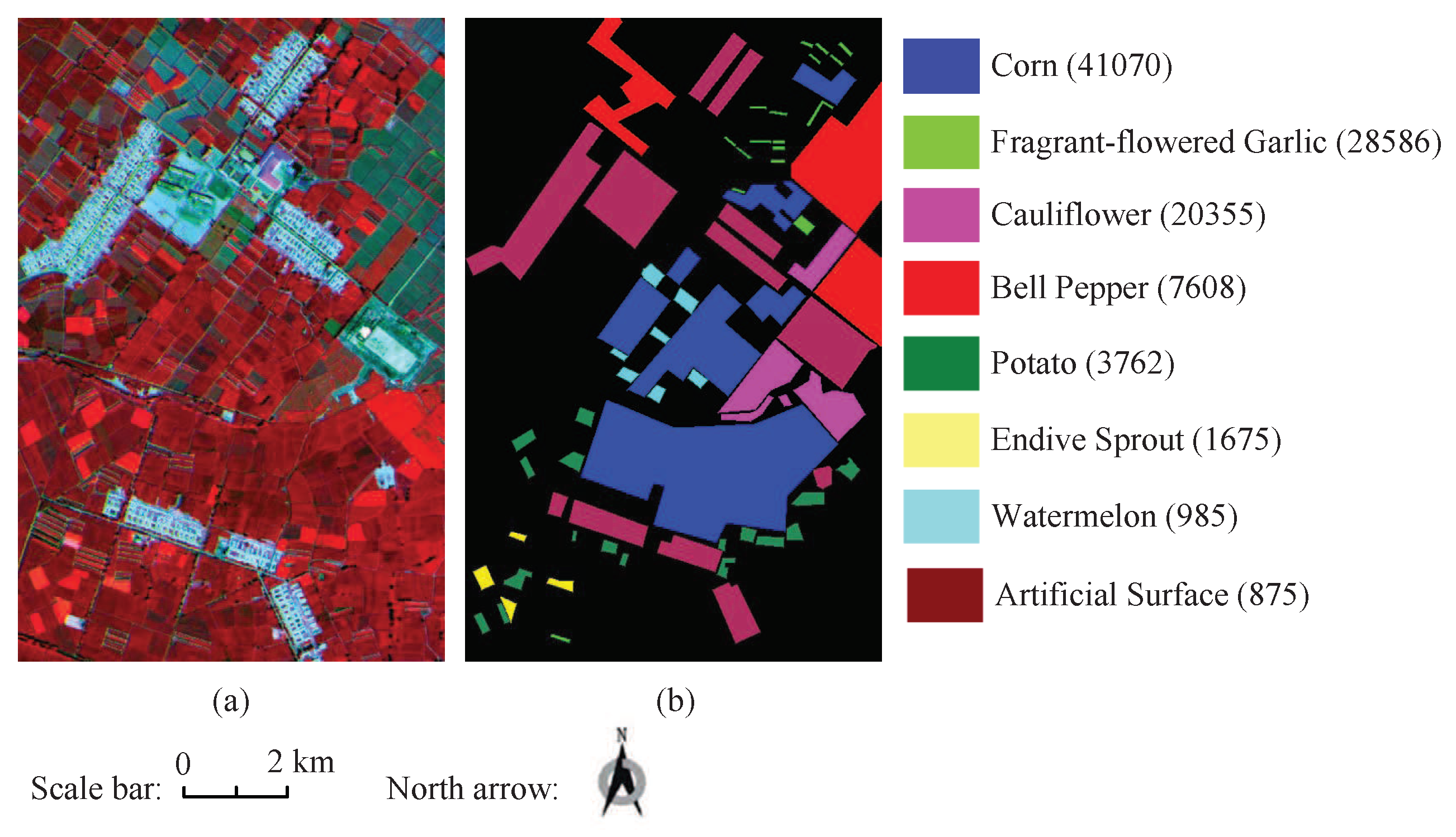
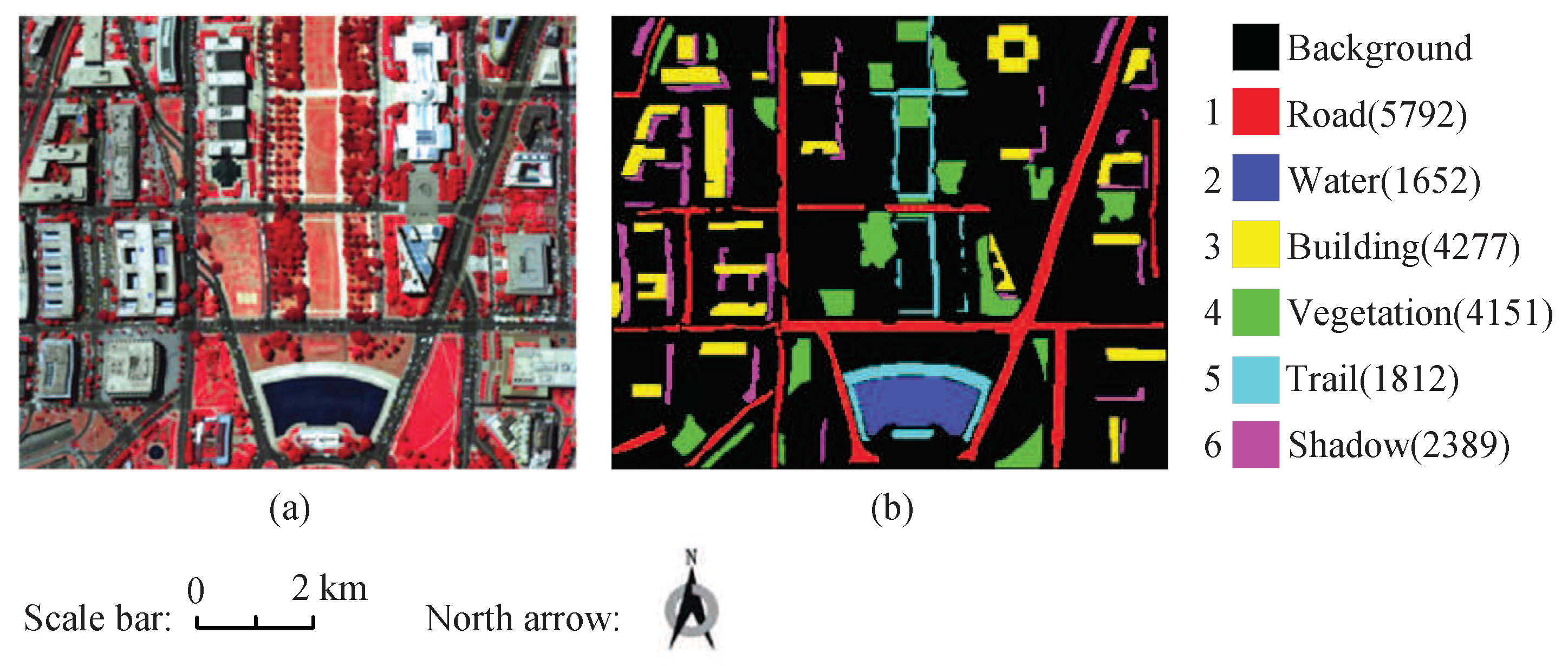
4.1. Experiment Data Set

PaviaU data set: This data set was captured on the city of Pavia, Italy by the ROSIS-03 (Reflective Optics Spectrographic Imaging System) airborne instrument. The ROSIS-03 sensor comprises 115 data channels with a spectral coverage ranging from 0.43 to 0.86 μ m. After removing water absorption bands, we adopted the remaining 103 bands for experiments. This data set was originally 610 × 340 pixels with a spatial resolution of 1.3 m. There are nine classes considered in the data set, that is, asphalt, meadows, gravel, trees, metal sheets, soil, bitumen, bricks and shadows. Figure 2 shows its false color scene and the corresponding ground truth.
Heihe data set [53,54]: This data set is captured by CASI/SASI sensors in Zhangye basin, Gansu Province, China. It is provided by Heihe Plan Science Data Center which is sponsored by the integrated research on the eco-hydrological process of the Heihe River Basin of the National Natural Science Foundation of China. The data set possesses a spatial size of 684 × 453 pixels with a geometric resolution of 2.4 m. Considering that 14 bands are easily absorbed by water absorption, the remaining 135 spectral bands are used for experiments. The data set contains 9 different land cover types. The scene in false color and its ground truth are shown in Figure 3.
Washington DC Mall data set: This data set is acquired by the airborne HYDICE from the mall in Washington DC. The spatial size of this data set is 250 × 307 pixels and the spatial resolution equals to 3 m per pixel. This data set covers a 0.4 μ m to 2.4 μ m spectral range with 210 bands. There are six different land cover types in the data set such as Road, Building, Trail and Vegetation. This scene in false color and its corresponding ground truth are shown in Figure 4.

4.2. Experimental Setup

In each experiment, we randomly divided the HSI data into training and test sets. Training set is used to construct a DR model and a test set is adopted to verify the effectiveness of the DR model. Then, the nearest neighbor classifier (NN) [55] was used for classification. After that, the classification accuracy of each class (CA), overall classification accuracy (OA), average classification accuracy (AA) and kappa coeffcient (KC) were adopted to evaluate the performance of different DR methods [47,52]. Among them, CA is the classification accuracy on each class of land covers, AA is a measure of the mean value of the classification accuracies of all classes, OA refers to the number of correctly classified instances divided by the total number of test samples, KC is a statistical measurement of consistency between the ground truth map and the final classification map. Suppose N i j is the number of samples in the j-th class that are classified into the i-th class, then the classification accuracy of i-th class (CA i ), AA, OA and KC can be defined as Equations (23)–(26):
CA i = N i i j = 1 c N j i
AA = 1 c i = 1 c CA i = 1 c i = 1 c N i i j = 1 c N j i
OA = 1 n i = 1 c N i i
KC = n i = 1 c N i i i = 1 c j = 1 c N j i × j = 1 c N i j n 2 i = 1 c j = 1 c N j i × j = 1 c N i j
in which c is the number of land cover types of HSI data and n is the total number of HSI pixels.
To evaluate the classification performance of the proposed SSMMDA algorithm, some state-of-art DR methods were selected for comparison, such methods include principal component analysis (PCA) [56], NPE [28], LPP [29], linear discriminant analysis (LDA) [57], maximum margin criterion (MMC) [58], MFA [31], nonparametric weighted feature extraction (NWFE) [59], sparsity preserving projections (SPP) [29], sparse discriminant embedding (SDE) [60], sparse manifold embedding (SME) [61], SMML [37], MMDA [33], DSSM [49], LPNPE [48] and weighted spatial-spectral and global-local discriminant analysis (WSSGLDA) [62]. RAW indicates that samples are classified without dimensionality reduction. The former twelve methods are spectral-based DR methods, they only consider the spectral information in HSI. The later three algorithms are spatial-spectral combined DR methods, which simultaneously consider the spectral information and spatial structure of HSI data. Among all the spectral-based DR algorithms, PCA, NPE, LPP, LDA, MMC and MFA are single manifold learning methods, while SMML and MMDA assume that the high dimensional HSI data lies on a multi-manifold structure.
In the experiments, we optimized the parameters to achieve good results for each method. For NPE, LPP, SMML and MMDA, we set the number of neighbors to 5. For MFA and DSSM, the number of intraclass and interclass neighbors were set to 7. For DSSM, LPNPE and WSSGLDA, the window size was set to 15 for PaviaU and Heihe data sets and 5 for the Washington DC data set. To reduce noise in the HSI, the HSI was pre-processed with a 5 × 5 spatial filter. For robustness, all the experiments were repeated for 10 times in each condition.

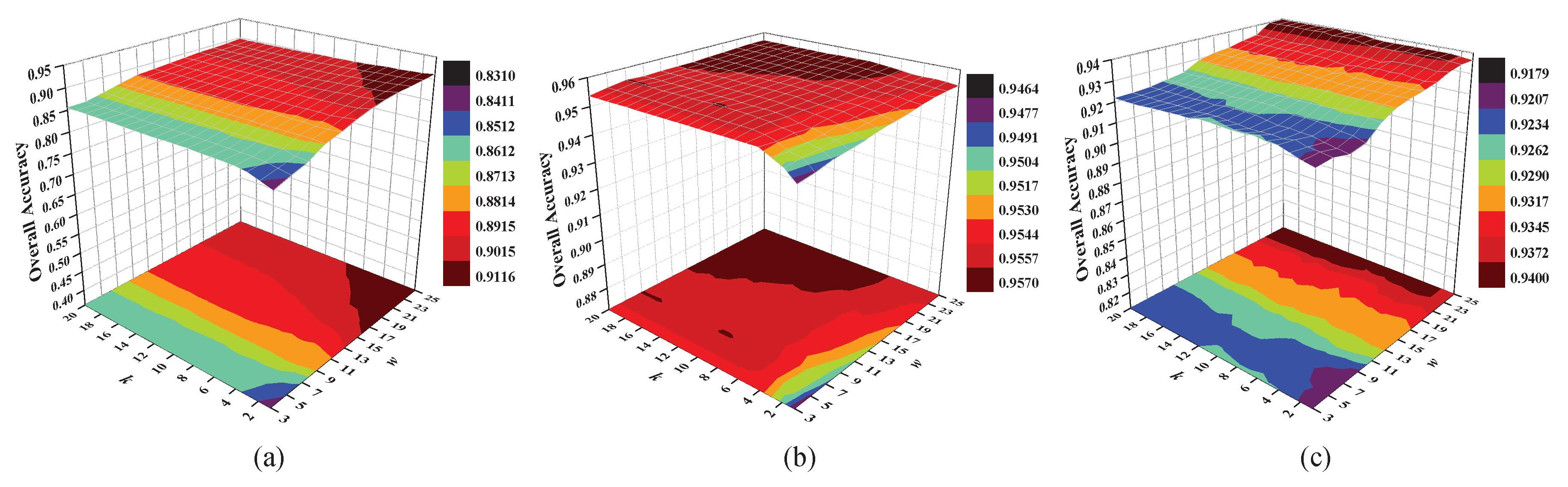
4.3. Analysis of Window Size w and Neighbor Number k
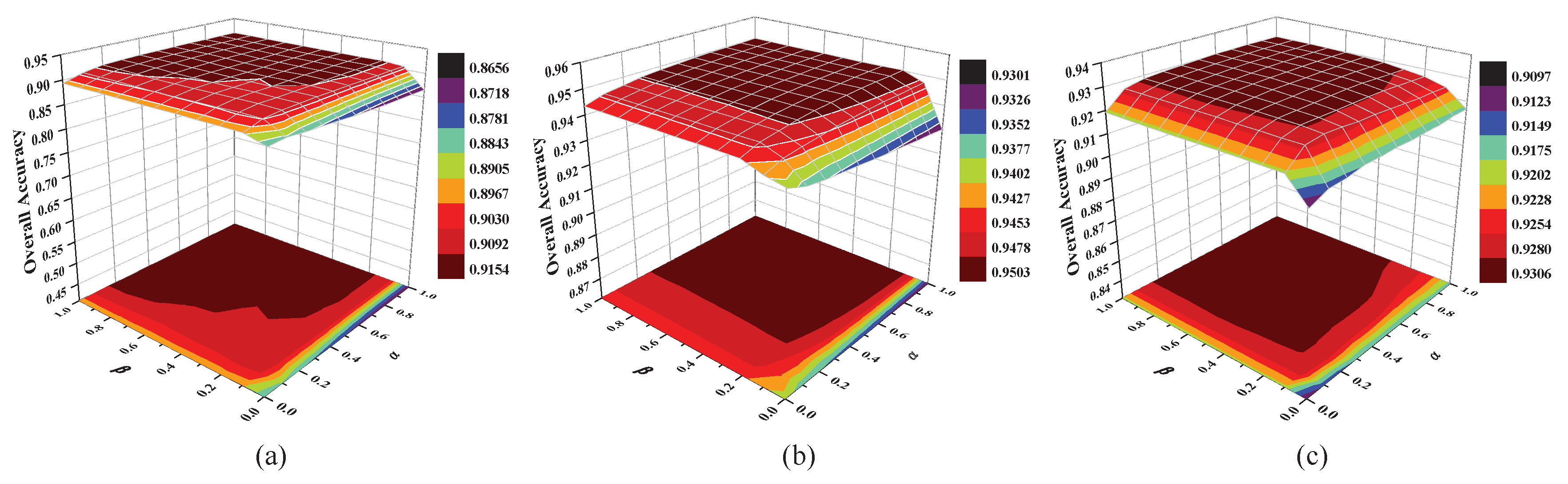
To investigate the classification performance of SSMMDA with different window size w and neighbor number k, 20 samples were randomly selected from each class as training set, and the remaining were used as test set. In the experiment, parameters w and k were chosen within a set of {3, 5, 7, …, 25} and a set of {1, 2, 3, …, 20}, respectively and the NN classifier were used to classify the test samples. Figure 5 shows the OAs versus different values of w and k.
As shown in Figure 5, as the window size w increases, the OAs first improve and then maintain a stable value. The reason is that a larger spatial window possesses more spatial neighbors, the neighbors can be utilized to construct a more effective DR model. However, if w is too large, the spatial information in neighbors will be redundant for DR of HSI. Therefore, the classification accuracies of SSMMDA will tend to remain stable. Besides, the classification accuracies improve with the increase of k and then slightly fluctuate. Because a small number of neighbor points cannot effectively reveal the multi-manifold structure of HSI in spectral domain, while a large k will produce too much useless information for adjacency graph construction. To balance running time and classification performance, we set w = 15, k = 5 for PaviaU data set, w = 15 and k = 8 for Heihe data set, and w = 17 and k = 8 for Washington DC Mall data set in the following experiments.

4.4. Analysis of Tradeoff Parameters α and β

SSMMDA has two tradeoff parameters α and β that are used to balance the contribution between the spectral information and spatial structure of HSI. To verify the classification performance of different values of α and β , we randomly selected 20 samples from each type of land covers for training and the rest were for testing. Parameters α and β were both tuned with a set of {0, 0.1, 0.2, 0.3, …, 0.9, 1}. After that, the NN classifier was used for classification. Figure 6 shows the average OAs with different α and β .
As can be seen from Figure 6, an increasing α causes a subtle change in terms of classification accuracy, because both spectral-domain intramanifold graph and spatial-domain intramanifold scatter matrix can enhance the intramanifold compactness and a suitable α can balance the contribution of spectral information and spatial structure in HSI. For parameter β , the OAs improve with the increase of β and then reach to a stable peak value, which indicates that the intermanifold scatter matrix can effectively enhance the intermanifold separability. To achieve better classification performance, we set α and β to 0.8 and 0.6 for the PaviaU data set, 0.9 and 0.6 for the Heihe and Washington DC Mall data sets in the experiments.

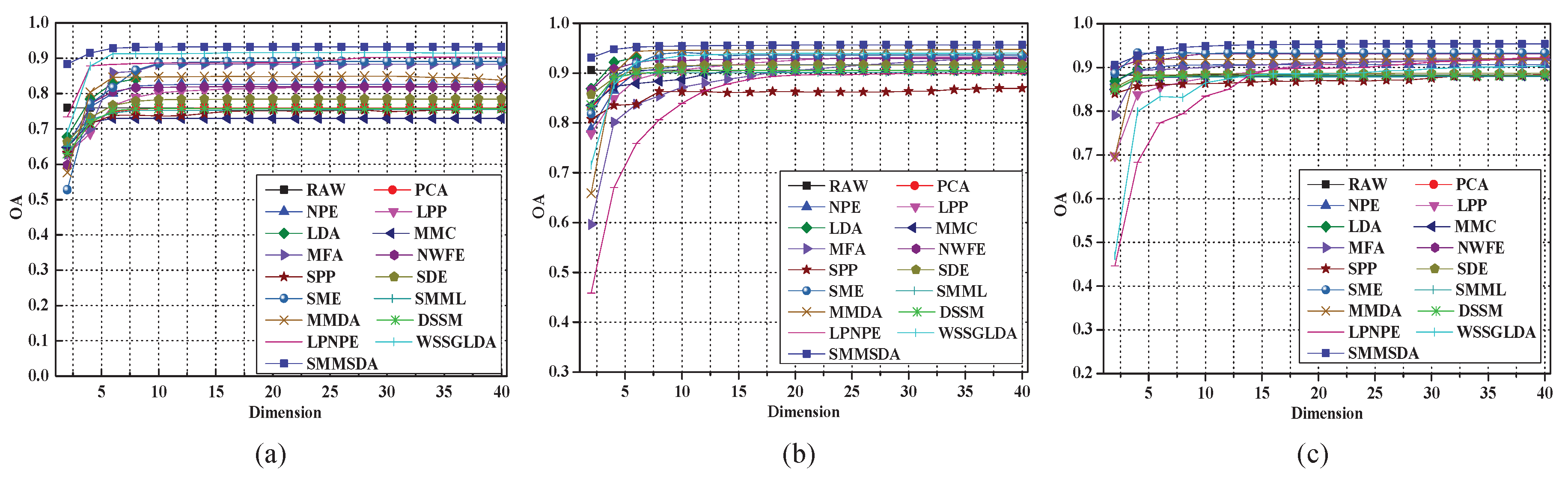
4.5. Investigation of Embedding Dimension d

The proposed SSMMDA method belongs to a dimensionality reduction method, thus we analyze the classification accuracy with different embedding dimensions d. To evaluate the influence of different embedding dimensions on classification performance, 30 samples per class were randomly chosen as training samples, the remaining were used as test samples. Figure 7 shows the classification results of different algorithms under different embedding dimensions.
In Figure 7, some similar conclusions can be obtained on the PaviaU, Heihe and Washington DC Mall data sets. When the value of d is lower than 15, the OAs of the DR algorithms increase significantly as the dimension increases. The reason is that a larger d means more discriminant features are utilized in the classification process, which is helpful to distinguish the land covers with similar spectrum. When d is larger than 15, the feature information contained in embedding space is close to saturation, an increasing d will not lead to the increase of the OAs. Besides, most DR methods can obtain better classification performance than RAW, which indicates that these algorithms can effectively reduce the useless information in HSI. To achieve better classification results for all algorithms, we set d = 30 for all DR methods on these three data sets and the dimension of LDA is c-1, c is the number of land cover types in each data set.

5. Analysis and Discussion

5.1. Analysis of Training Sample Size

To investigate the classification performance of the algorithms under different number of training samples, n i (n i = 10, 20, 30, 40, 50, 60) samples were randomly selected from each class for training, and the rest of the samples were used for testing. For robustness, all the experiments were repeated for 10 times in each condition. Table 1, Table 2 and Table 3 report the classification results of different DR methods with different number of training samples on the PaviaU, Heihe and Washington DC Mall data sets.
According to Table 1, Table 2 and Table 3, the OAs of the above algorithms are significantly improved as n i increases. The reason is that a large number of training samples contain more abundant feature information, which is conducive to the feature learning of HSI data. For single manifold algorithms with spectral information, supervised methods of LDA, SME and MFA, are superior to unsupervised ones such as PCA, NPE, LPP and SPP, it indicates that the priori label information of HSI is helpful to improve the classification performance of HSI. For the single manifold-based DR algorithms, most spatial-spectral combined methods achieve higher classification accuracies than the spectral DR methods. Because the HSI possesses the spatial consistency property and pixels from the same class are commonly distributed in blocks. Therefore, the spatial information is of great significance to improve the feature representation and classification performance of HSI. For the multiple manifold-based DR algorithms, the proposed SSMMDA method achieves better classification results than SMML and MMDA in most conditions, this is because SMML and MMDA only consider the spectral information of HSI and they do not utilize the spatial structure to further enhance the classification performance. For all the DR methods, SSMMDA has the better OAs and KCs than the other algorithms, because it simultaneously considers the multi-manifold structure and the spatial-spectral combined information in HSI.

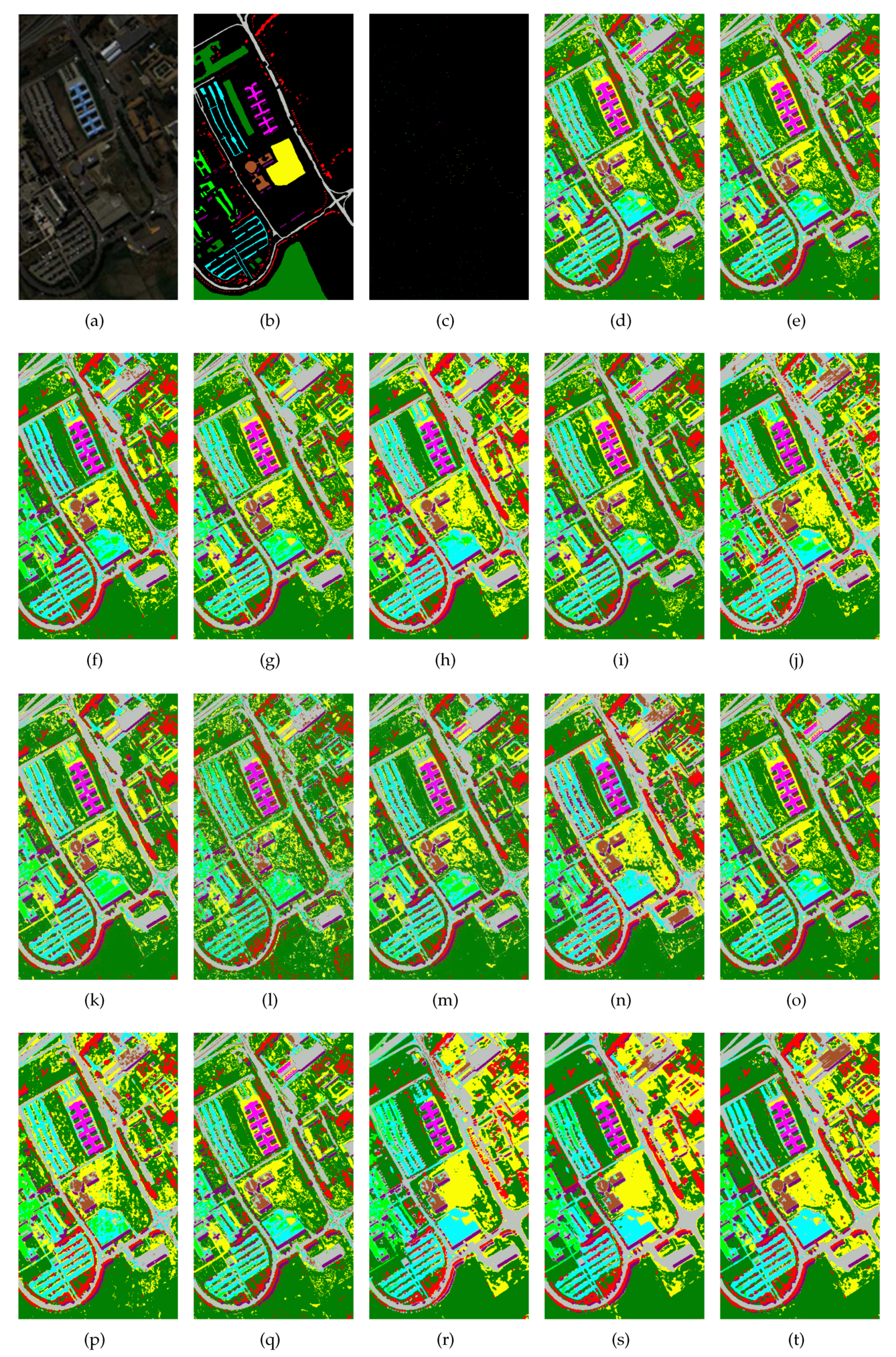
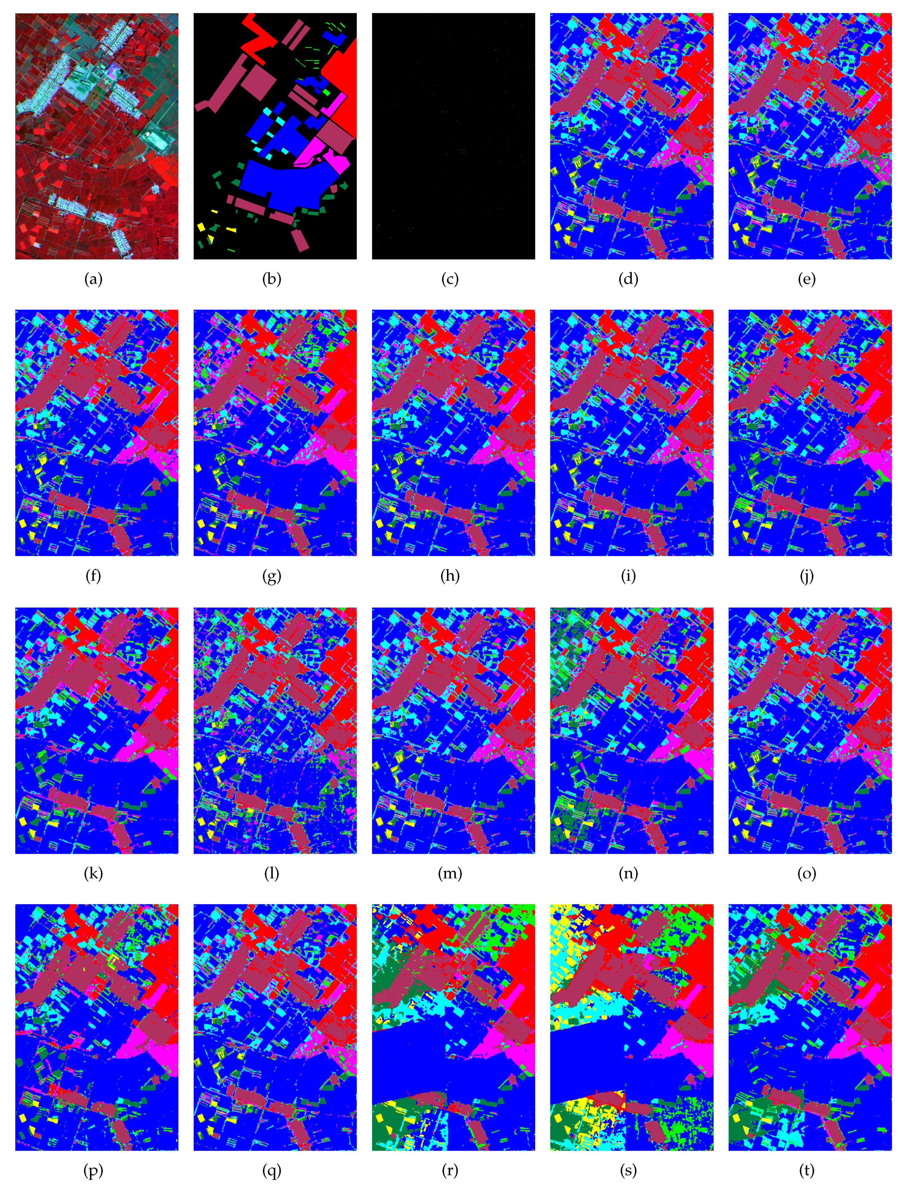
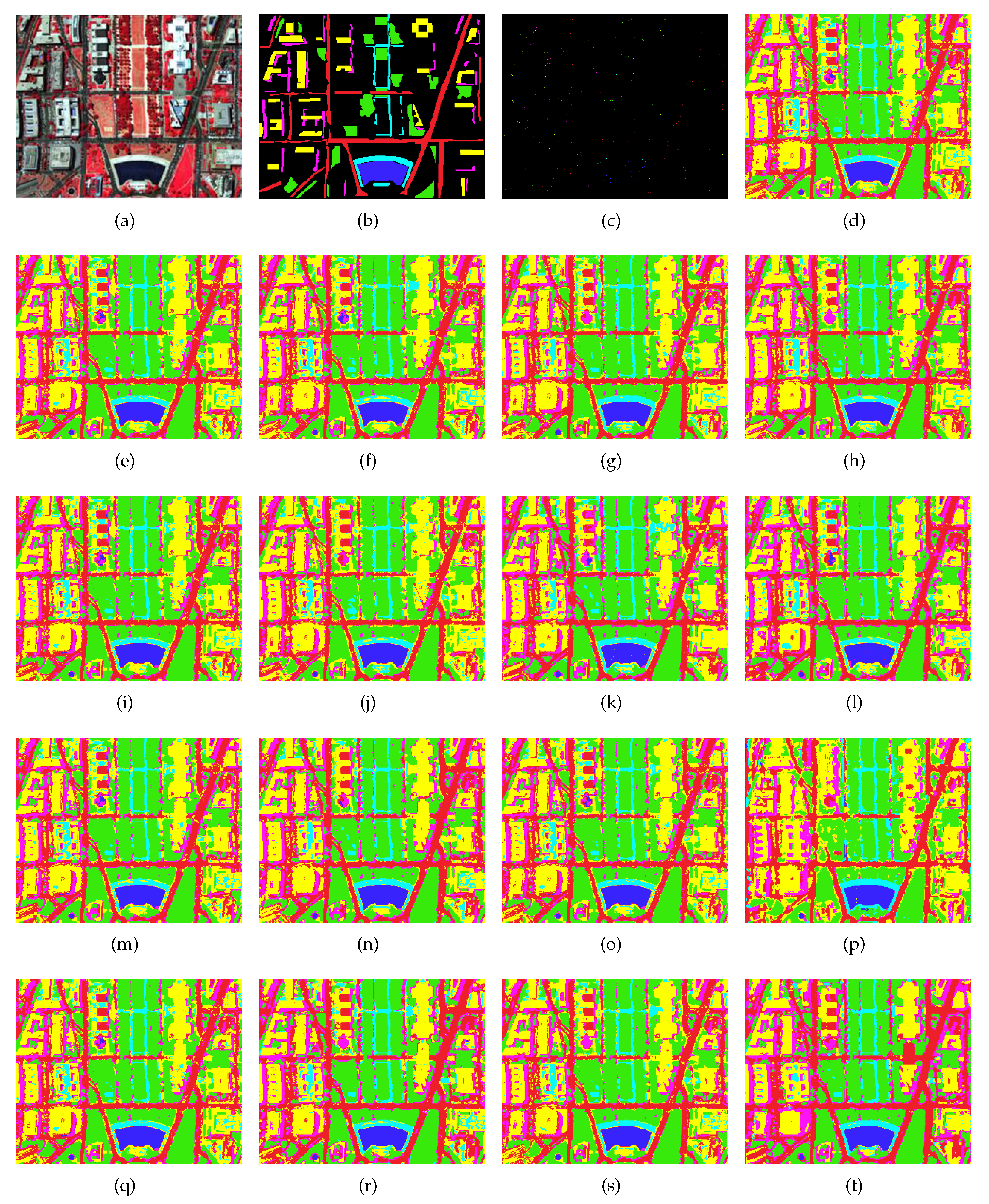
5.2. Analysis of Classification Results

To explore the classification performance of SSMMDA on each class, we randomly selected a percentage of samples per class as training set and the remaining samples were used as a test set. The training set is used to construct a DR model and the test set is adopted to verify the effectiveness of the DR model. In the experiments, we set the percentage to 0.5% for the PaviaU data set, 0.1% for the Heihe data set and 1% for the Washington DC Mall data set. The CAs, OAs, AAs and KCs of different methods on the PaviaU, Heihe, Washington DC Mall data sets are detailed in Table 4, Table 5 and Table 6, respectively, and Figure 8, Figure 9 and Figure 10 show the corresponding classification maps of different algorithms on these three data sets.
As shown in Table 4, Table 5 and Table 6, SSMMDA achieved better classification results than other algorithms in most classes and it possessed the best OA, AA and KC on the three HSI datasets. This indicates that the proposed SSMMDA method has a stronger ability to characterize the geometric relations between samples and extract more effective spatial-spectral combined information for classification. Besides, the classification maps of SSMMDA in Figure 8, Figure 9 and Figure 10 produced more homogenous regions than the other methods, especially in the classes of Asphalt, Bitumen and Bricks for the PaviaU data set, Corn, Watermelon and Artificial Surface for the Heihe data set and Road, Water, Building and Shadow for the Washington DC Mall data set. The reason is that SSMMDA not only explores the multiple manifold structure of HSI data but also utilizes the spatial-spectral combined information to extract the discriminant features, which is conducive to the classification of HSI data.

5.3. Analysis of Computational Efficiency

To quantitatively compare the computational efficiency of each algorithm, we show the computational time of each algorithm in Table 7, where 30 labeled samples per class were selected for training, and the remaining samples were for testing. All the results in Table 7 were obtained on a personal computer, which has the i3-7100 CPU and 12-G memory. Besides, the version of Windows system and MATLAB are 64-bit Windows 10 and 2017a, respectively.
As shown in Table 7, the proposed SSMMDA method requires more time in the classification process of HSI. The reason is that SSMMDA simultaneously considers the spatial and spectral information and it needs to build two models in both the spatial domain and the spectral domain. Besides, Since SSMMDA has c different mapping matrices, it needs to project the samples into c low-dimensional spaces when calculating the embedding features of samples, so the computational complexity of SSMMDA is slightly increased. However, the slight increase in computational complexity is acceptable relative to the improvement for classification performance.

6. Conclusions

High-dimensional data can be divided into different subsets; each subset is located on a particular submanifold. Traditional feature learning methods can not effectively discover the multi-manifold structure in hyperspectral image, which restricts their classification performance of HSI. In this paper, we proposed a new DR method termed spatial-spectral multiple manifold discriminant analysis (SSMMDA) for the classification on HSI data. SSMMDA first divides the HSI data into several different subsets according to the label information of training samples. Then, it constructs an intramanifold graph for each submanifold to characterize the within-manifold similarity in spectral domain and designs an intramanifold scatter matrix and an intermanifold scatter matrix for each submanifold to characterize the within-manifold similarity and the between-manifold dissimilarity in the spatial domain. After that, a new spatial-spectral combined DR model is built for each submanifold to obtain an optimal projection, and the discriminative features on different submanifolds are fused to enhance the classification performance. Experiments on PaviaU, Heihe and Washington DC Mall hyperspectral data sets demonstrate that the proposed SSMMDA method can obtain effective discriminative features and significantly improve the classification performance of HSI. In our future work, we will focus on how to obtain the optimum embedding dimension for each submanifold to further improve the classification performance of HSI.

Author Contributions

G.S. carried out the experiments and finished the first version of this manuscript. H.H. and J.L. was primarily responsible for mathematical modeling and experimental design. Z.L. and L.W. provided important suggestions to improve the paper.

Funding

This work was supported by the Basic and Frontier Research Programmes of Chongqing under Grant cstc2018jcyjAX0093, the Fundamental Research Funds for the Central Universities under Grant 2019CDYGYB008, and the graduate research and innovation foundation of Chongqing under Grants CYB19039 and CYS18035.

Acknowledgments

The authors would like to thank the anonymous reviewers and associate editor for their valuable comments and suggestions to improve the quality of the paper.

Conflicts of Interest

The authors declare no conflict of interest.

References

  1. Li, S.T.; Hao, Q.B.; Kang, X.; Benediktsson, J.A. Gaussian Pyramid Based Multiscale Feature Fusion for Hyperspectral Image Classification. IEEE J. Sel. Top. Appl. Earth Obs. Remote Sens. 2018, 11, 3312–3324. [Google Scholar] [CrossRef]
  2. Zhai, H.; Zhang, H.Y.; Zhang, L.P.; Li, P.X. Laplacian-Regularized Low-Rank Subspace Clustering for Hyperspectral Image Band Selection. IEEE Trans. Geosci. Remote Sens. 2018, 57, 1723–1740. [Google Scholar] [CrossRef]
  3. Luo, F.L.; Zhang, L.P.; Zhou, X.C.; Guo, T.; Cheng, Y.X.; Yin, T.L. Sparse-Adaptive Hypergraph Discriminant Analysis for Hyperspectral Image Classification. IEEE Geosci. Remote Sens. Lett. 2019, 99, 1–5. [Google Scholar] [CrossRef]
  4. Peng, J.T.; Du, Q. Robust joint sparse representation based on maximum correntropy criterion for hyperspectral image classification. IEEE Trans. Geosci. Remote Sens. 2017, 55, 7152–7164. [Google Scholar] [CrossRef]
  5. Li, W.; Wu, G.D.; Du, Q. Transferred Deep Learning for Anomaly Detection in Hyperspectral Imagery. IEEE Trans. Geosci. Remote Sens. 2017, 14, 597–601. [Google Scholar] [CrossRef]
  6. Hu, F.; Xia, G.S.; Wang, Z.F.; Huang, X.; Zhang, L.P.; Sun, H. Unsupervised feature learning via spectral clustering of patches for remotely sensed scene classification. IEEE J. Sel. Top. Appl. Earth Obs. Remote Sens. 2015, 8, 2015–2030. [Google Scholar] [CrossRef]
  7. Song, W.W.; Li, S.T.; Fang, L.Y.; Lu, T. Hyperspectral Image Classification with Deep Feature Fusion Network. IEEE Trans. Geosci. Remote Sens. 2016, 54, 4544–4554. [Google Scholar] [CrossRef]
  8. Zhai, H.; Zhang, H.Y.; Zhang, L.P.; Li, P.X. Total Variation Regularized Collaborative Representation Clustering with a Locally Adaptive Dictionary for Hyperspectral Imagery. IEEE Trans. Geosci. Remote Sens. 2018, 57, 166–180. [Google Scholar] [CrossRef]
  9. Yuan, Y.; Zheng, X.T.; Lu, X.Q. Discovering diverse subset for unsupervised hyperspectral band selection. IEEE Trans. Image Process. 2017, 26, 51–64. [Google Scholar] [CrossRef]
  10. Jia, S.; Tang, G.H.; Zhu, J.S.; Li, Q.Q. A Novel Ranking-Based Clustering Approach for Hyperspectral Band Selection. IEEE Trans. Geosci. Remote Sens. 2016, 54, 88–102. [Google Scholar] [CrossRef]
  11. Dong, Y.N.; Du, B.; Zhang, L.P.; Zhang, L.F. Dimensionality reduction and classification of hyperspectral images using ensemble discriminative local metric learning. IEEE Trans. Geosci. Remote Sens. 2017, 55, 2509–2524. [Google Scholar] [CrossRef]
  12. Luo, Y.; Wen, Y.G.; Tao, D.C.; Gui, J.; Xu, C. Large Margin Multi-Modal Multi-Task Feature Extraction for Image Classification. IEEE Trans. Image Process. 2016, 25, 414–427. [Google Scholar] [CrossRef]
  13. Hang, R.L.; Liu, Q.S.; Sun, Y.B.; Yuan, X.T.; Pei, H.C.; Plaza, J.; Plaza, A. Robust matrix discriminative analysis for feature extraction from hyperspectral images. IEEE J. Sel. Top. Appl. Earth Obs. Remote Sens. 2017, 10, 2002–2011. [Google Scholar] [CrossRef]
  14. Li, Q.; Ji, H.B. Multimodality image registration using local linear embedding and hybrid entropy. Neurocomputing 2013, 111, 34–42. [Google Scholar] [CrossRef]
  15. Tu, S.T.; Chen, J.Y.; Yang, W.; Sun, H. Laplacian Eigenmaps-Based Polarimetric Dimensionality Reduction for SAR Image Classification. IEEE Trans. Geosci. Remote Sens. 2012, 50, 170–179. [Google Scholar] [CrossRef]
  16. Li, W.; Zhang, L.P.; Zhang, L.F.; Du, B. GPU Parallel Implementation of Isometric Mapping for Hyperspectral Classification. IEEE Geosci. Remote Sens. Lett. 2017, 14, 1532–1536. [Google Scholar] [CrossRef]
  17. Chen, J.; Liu, Y. Locally linear embedding: A survey. Artif. Intell. Rev. 2011, 36, 29–48. [Google Scholar] [CrossRef]
  18. Belkin, M.; Niyogi, P. Laplacian Eigenmaps for Dimensionality Reduction and Data Representation. Neural Comput. 2003, 15, 1373–1396. [Google Scholar] [CrossRef] [Green Version]
  19. Feilhauer, H.; Faude, U.; Schmidtlein, S. Combining Isomap ordination and imaging spectroscopy to map continuous floristic gradients in a heterogeneous landscape. Remote Sens. Environ. 2011, 115, 2513–2524. [Google Scholar] [CrossRef]
  20. Sun, W.W.; Yang, G.; Du, B.; Zhang, L.F.; Zhang, L.P. A sparse and low-rank near-isometric linear embedding method for feature extraction in hyperspectral imagery classification. IEEE Trans. Geosci. Remote Sens. 2017, 55, 4032–4046. [Google Scholar] [CrossRef]
  21. Huang, H.; Li, Z.Y.; Pan, Y.S. Multi-Feature Manifold Discriminant Analysis for Hyperspectral Image Classification. Remote Sens. 2019, 11, 651. [Google Scholar] [CrossRef]
  22. Fang, L.Y.; Wang, C.; Li, S.T.; Beneditsson, J.A. Hyperspectral image classification via multiple-feature- based adaptive sparse representation. IEEE Trans. Instrum. Meas. 2017, 7, 1646–1657. [Google Scholar] [CrossRef]
  23. Wang, Q.; Wan, J.; Yuan, Y. Locality Constraint Distance Metric Learning for Traffic Congestion Detection. Pattern Recognit. 2018, 9, 272–281. [Google Scholar] [CrossRef]
  24. Feng, F.B.; Li, W.; Du, Q.; Zhang, B. Dimensionality reduction of hyperspectral image with graph-based discriminant analysis considering spectral similarity. Remote Sens. 2017, 9, 323. [Google Scholar] [CrossRef]
  25. Gui, J.; Sun, Z.N.; Jia, W.; Hu, R.X.; Lei, Y.K.; Ji, S.W. Discriminant sparse neighborhood preserving embedding for face recognition. Pattern Recognit. 2012, 45, 2884–2893. [Google Scholar] [CrossRef]
  26. Wong, W.K.; Zhao, H.T. Supervised optimal locality preserving projection. Pattern Recognit. 2012, 45, 186–197. [Google Scholar] [CrossRef]
  27. Zhang, X.R.; He, Y.D.; Zhou, N.; Zheng, Y.G. Semisupervised Dimensionality Reduction of Hyperspectral Images via Local Scaling Cut Criterion. IEEE Geosci. Remote Sens. Lett. 2013, 10, 1547–1551. [Google Scholar] [CrossRef]
  28. Lu, G.F.; Jin, Z.; Zou, J. Face recognition using discriminant sparsity neighborhood preserving embedding. Knowl.-Based Syst. 2012, 31, 119–127. [Google Scholar] [CrossRef]
  29. Qiao, L.S.; Chen, S.C.; Tan, X.Y. Sparsity preserving projections with applications to face recognition. Pattern Recognit. 2010, 43, 331–341. [Google Scholar] [CrossRef] [Green Version]
  30. Mohanty, R.; Happy, S.L.; Routray, A. A Semisupervised Spatial Spectral Regularized Manifold Local Scaling Cut With HGF for Dimensionality Reduction of Hyperspectral Images. IEEE Trans. Geosci. Remote Sens. 2019, 57, 3423–3435. [Google Scholar] [CrossRef] [Green Version]
  31. Pang, Y.W.; Ji, Z.; Jing, P.G.; Li, X.L. Ranking Graph Embedding for Learning to Rerank. IEEE Trans. Neural Netw. Learn. Syst. 2013, 24, 1292–1303. [Google Scholar] [CrossRef] [PubMed]
  32. Luo, F.L.; Huang, H.; Duan, Y.L.; Liu, J.M.; Liao, Y.H. Local Geometric Structure Feature for Dimensionality Reduction of Hyperspectral Imagery. Remote Sens. 2017, 9, 790. [Google Scholar] [CrossRef]
  33. Yang, W.K.; Sun, C.Y.; Zhang, L. A multi-manifold discriminant analysis method for image feature extraction. Pattern Recognit. 2011, 44, 1649–1657. [Google Scholar] [CrossRef] [Green Version]
  34. Hettiarachchi, R.; Peters, J.F. Multi-manifold LLE learning in pattern recognition. Pattern Recognit. 2015, 48, 2947–2960. [Google Scholar] [CrossRef]
  35. Jiang, J.J.; Hu, R.M.; Wang, Z.Y.; Cai, Z.H. CDMMA: Coupled discriminant multi-manifold analysis for matching low-resolution face images. Signal Process. 2016, 124, 162–172. [Google Scholar] [CrossRef]
  36. Chu, Y.J.; Zhao, L.D.; Ahmad, T. Multiple feature subspaces analysis for single sample per person face recognition. Vis. Comput. 2019, 35, 239–256. [Google Scholar] [CrossRef]
  37. Shi, L.K.; Hao, J.S.; Zhang, X. Image recognition method based on supervised multi-manifold learning. J. Intell. Fuzzy Syst. 2017, 32, 2221–2232. [Google Scholar] [CrossRef]
  38. Jiang, J.J.; Ma, J.Y.; Chen, C.; Wang, Z.Y.; Cai, Z.H.; Wang, L.Z. SuperPCA: A Superpixelwise PCA Approach for Unsupervised Feature Extraction of Hyperspectral Imagery. IEEE Trans. Geosci. Remote Sens. 2018, 56, 4581–4593. [Google Scholar] [CrossRef] [Green Version]
  39. Tu, B.; Zhang, X.F.; Kang, X.D.; Wang, J.P.; Benediktsson, J.A. Spatial Density Peak Clustering for Hyperspectral Image Classification with Noisy Labels. IEEE Trans. Geosci. Remote Sens. 2019, 57, 5085–5097. [Google Scholar] [CrossRef]
  40. Fang, L.Y.; Zhuo, H.J.; Li, S.T. Super-resolution of hyperspectral image via superpixel-based sparse representation. Neurocomputing 2018, 273, 171–177. [Google Scholar] [CrossRef]
  41. Zhao, W.Z.; Du, S.H. Spectral-Spatial Feature Extraction for Hyperspectral Image Classification: A Dimension Reduction and Deep Learning Approach. IEEE Trans. Geosci. Remote Sens. 2016, 54, 4544–4554. [Google Scholar] [CrossRef]
  42. He, L.; Li, J.; Liu, C.Y.; Li, S.T. Recent advances on spectral-spatial hyperspectral image classification: An overview and new guidelines. IEEE Trans. Geosci. Remote Sens. 2018, 56, 1579–1597. [Google Scholar] [CrossRef]
  43. Zhang, L.F.; Zhang, Q.; Du, B.; Huang, X.; Tang, Y.Y.; Tao, D.C. Simultaneous Spectral-Spatial Feature Selection and Extraction for Hyperspectral Images. IEEE Trans. Cybern. 2018, 48, 16–28. [Google Scholar] [CrossRef] [PubMed]
  44. Liao, W.Z.; Mura, M.D.; Chanussot, J.; Pizurica, A. Fusion of spectral and spatial information for classification of hyperspectral remote sensed imagery by local graph. IEEE J. Sel. Top. Appl. Earth Obs. Remote Sens. 2018, 9, 583–594. [Google Scholar] [CrossRef]
  45. Kang, X.D.; Li, S.T.; Benediktsson, J.A. Feature extraction of hyperspectral images with image fusion and recursive filtering. IEEE Geosci. Remote Sens. Lett. 2014, 52, 3742–3752. [Google Scholar] [CrossRef]
  46. Huang, H.; Shi, G.Y.; He, H.B.; Duan, Y.L.; Luo, F.L. Dimensionality Reduction of Hyperspectral Imagery Based on Spatial-spectral Manifold Learning. IEEE Trans. Cybern. 2019, 1–14. [Google Scholar] [CrossRef]
  47. Luo, F.L.; Du, B.; Zhang, L.P.; Zhang, L.F.; Tao, D.C. Feature Learning Using Spatial-Spectral Hypergraph Discriminant Analysis for Hyperspectral Image. IEEE Trans. Cybern. 2019, 49, 2406–2419. [Google Scholar] [CrossRef]
  48. Zhou, Y.C.; Peng, J.T.; Chen, C.L.P. Dimension reduction using spatial and spectral regularized local discriminant embedding for hyperspectral image classification. IEEE Trans. Geosci. Remote Sens. 2015, 53, 1082–1095. [Google Scholar] [CrossRef]
  49. Feng, Z.X.; Yang, S.Y.; Wang, S.G.; Jiao, L.C. Discriminative Spectral-Spatial Margin-Based Semisupervised Dimensionality Reduction of Hyperspectral Data. IEEE Geosci. Remote Sens. Lett. 2015, 12, 224–228. [Google Scholar] [CrossRef]
  50. Mohanty, R.; Happy, S.L.; Routray, A. Spatial-Spectral Regularized Local Scaling Cut for Dimensionality Reduction in Hyperspectral Image Classification. IEEE Geosci. Remote Sens. Lett. 2019, 16, 932–936. [Google Scholar] [CrossRef]
  51. Sellami, A.; Farah, I.R. High-level hyperspectral image classification based on spectro-spatial dimensionality reduction. Spat. Stat. 2016, 16, 103–117. [Google Scholar] [CrossRef]
  52. Huang, H.; Chen, M.L.; Duan, Y.L. Dimensionality Reduction of Hyperspectral Image Using Spatial-Spectral Regularized Sparse Hypergraph Embedding. Remote Sens. 2019, 11, 1039. [Google Scholar] [CrossRef]
  53. Xiao, Q.; Wen, J.G. HiWATER: Thermal-Infrared Hyperspectral Radiometer (4th, July, 2012). Heihe Plan Sci. Data Center 2013. [Google Scholar] [CrossRef]
  54. Xue, Z.H.; Su, H.J.; Du, P.J. Sparse graph regularization for robust crop mapping using hyperspectral remotely sensed imagery: A case study in Heihe Zhangye oasis. In Proceedings of the 2016 IEEE International Geoscience and Remote Sensing Symposium (IGARSS), Beijing, China, 10–15 July 2016; pp. 779–782. [Google Scholar] [CrossRef]
  55. Li, W.; Du, Q.; Zhang, F.; Hu, W. Collaborative-representation-based nearest neighbor classifier for hyperspectral imagery. IEEE Geosci. Remote Sens. Lett. 2015, 12, 389–393. [Google Scholar] [CrossRef]
  56. Datta, A.; Ghosh, S.; Ghosh, A. Unsupervised band extraction for hyperspectral images using clustering and kernel principal component analysis. Int. J. Remote Sens. 2017, 38, 850–873. [Google Scholar] [CrossRef]
  57. Liao, W.Z.; Pizurica, A.; Scheunders, P.; Philips, W.; Pi, Y.G. Semisupervised Local Discriminant Analysis for Feature Extraction in Hyperspectral Images. IEEE Trans. Geosci. Remote Sens. 2013, 51, 184–198. [Google Scholar] [CrossRef]
  58. Li, H.F.; Jiang, T.; Zhang, K.S. Efficient and robust feature extraction by maximum margin criterion. IEEE Trans. Neural Netw. 2006, 17, 157–165. [Google Scholar] [CrossRef]
  59. Kuo, B.C.; Landgrebe, D.A. Nonparametric weighted feature extraction for classification. IEEE Trans. Geosci. Remote Sens. 2004, 42, 1096–1105. [Google Scholar] [CrossRef]
  60. Huang, H. Classification of hyperspectral remote-sensing images based on sparse manifold learning. J. Appl. Remote Sens. 2013, 7, 073464. [Google Scholar] [CrossRef]
  61. Huang, H.; Luo, F.L.; Liu, J.M.; Yang, Y.Q. Dimensionality reduction of hyperspectral images based on sparse discriminant manifold embedding. ISPRS-J. Photogramm. Remote Sens. 2015, 106, 42–54. [Google Scholar] [CrossRef]
  62. Zeng, S.; Wang, Z.Y.; Gao, C.J.; Kang, Z.; Feng, D.G. Hyperspectral Image Classification With Global-Local Discriminant Analysis and Spatial-Spectral Context. IEEE J. Sel. Top. Appl. Earth Obs. Remote Sens. 2018, 11, 5005–5018. [Google Scholar] [CrossRef]
Figure 1. The flowchart of the proposed spatial-spectral multi-manifold discriminant analysis (SSMMDA) method.
Remotesensing 11 02414 g001
Figure 2. PaviaU hyperspectral image (HSI). (a) HSI in false-color; (b) Ground-truth map.
Remotesensing 11 02414 g002
Figure 3. Heihe hyperspectral image. (a) HSI in false-color; (b) Ground-truth map.
Remotesensing 11 02414 g003
Figure 4. Washington DC Mall hyperspectral image. (a) HSI in false-color; (b) Ground-truth map.
Remotesensing 11 02414 g004
Figure 5. Overall classification accuracies (OAs) with different window sizes w and neighbor number k. (a) PaviaU. (b) Heihe. (c) Washington DC Mall.
Remotesensing 11 02414 g005
Figure 6. OAs with different tradeoff parameters α and β . (a) PaviaU. (b) Heihe. (c) Washington DC Mall.
Remotesensing 11 02414 g006
Figure 7. OAs with different embedding dimensions d. (a) PaviaU. (b) Heihe. (c) Washington DC Mall.
Remotesensing 11 02414 g007
Figure 8. Classification maps of different methods on the PaviaU data set. (a) False color image; (b) Ground truth; (c) Training samples; (d) RAW; (e) PCA; (f) NPE; (g) LPP; (h) LDA; (i) MMC; (j) MFA; (k) NWFE; (l) SPP; (m) SDE; (n) SME; (o) SMML; (p) MMDA; (q) DSSM; (r) LPNPE; (s) WSSGLDA; (t) SSMMDA.
Remotesensing 11 02414 g008
Figure 9. Classification maps of different methods on the Heihe data set. (a) False color image; (b) Ground truth; (c) Training samples; (d) RAW; (e) PCA; (f) NPE; (g) LPP; (h) LDA; (i) MMC; (j) MFA; (k) NWFE; (l) SPP; (m) SDE; (n) SME; (o) SMML; (p) MMDA; (q) DSSM; (r) LPNPE; (s) WSSGLDA; (t) SSMMDA.
Remotesensing 11 02414 g009
Figure 10. Classification maps of different methods on the Washington DC Mall data set. (a) False color image; (b) Ground truth; (c) Training samples; (d) RAW; (e) PCA; (f) NPE; (g) LPP; (h) LDA; (i) MMC; (j) MFA; (k) NWFE; (l) SPP; (m) SDE; (n) SME; (o) SMML; (p) MMDA; (q) DSSM; (r) LPNPE; (s) WSSGLDA; (t) SSMMDA.
Remotesensing 11 02414 g010
Table 1. Classification results with different values of n i on the PaviaU dataset with nearest neighbor (NN) classifier. Each method has two rows, where the first row is the OA ± STD (%) and the second row is the Kappa coefficient (KC).
Algorithm102030405060
RAW67.71 + 3.44
(0.601)
73.53 + 2.51
(0.669)
76.49 + 1.62
(0.703)
78.41 + 1.42
(0.726)
79.72 ± 1.56
(0.742)
82.25 ± 1.26
(0.772)
PCA [56]67.71 ± 3.44
(0.601)
73.53 ± 2.51
(0.669)
76.49 ± 1.61
(0.703)
78.40 ± 1.42
(0.726)
79.71 ± 1.57
(0.742)
82.24 ± 1.26
(0.772)
NPE [28]73.62 ± 3.84
(0.670)
80.15 ± 2.73
(0.748)
84.30 ± 1.75
(0.798)
86.34 ± 2.13
(0.824)
88.37 ± 2.05
(0.850)
90.36 ± 1.82
(0.874)
LPP [29]75.88 ± 2.25
(0.698)
82.96 ± 1.43
(0.782)
85.27 ± 0.67
(0.810)
86.47 ± 1.66
(0.826)
87.37 ± 1.56
(0.837)
89.32 ± 1.83
(0.861)
LDA [57]75.59 ± 3.51
(0.696)
80.60 ± 1.66
(0.754)
86.66 ± 1.75
(0.827)
88.32 ± 1.57
(0.848)
90.43 ± 1.69
(0.875)
91.68 ± 1.25
(0.891)
MMC [58]67.03 ± 3.18
(0.593)
70.94 ± 2.79
(0.638)
73.10 ± 1.73
(0.662)
74.95 ± 1.34
(0.684)
75.94 ± 1.66
(0.697)
78.14 ± 1.50
(0.722)
MFA [31]79.67 ± 3.54
(0.742)
86.40 ± 1.95
(0.824)
88.63 ± 1.68
(0.852)
89.31 ± 1.52
(0.861)
90.53 ± 2.11
(0.876)
92.46 ± 1.44
(0.901)
NWFE [59]73.07 ± 3.79
(0.664)
78.89 ± 1.92
(0.733)
82.89 ± 1.85
(0.78)
83.15 ± 1.78
(0.784)
84.61 ± 1.87
(0.802)
85.35 ± 1.45
(0.811)
SPP [29]60.83 ± 3.74
(0.519)
66.62 ± 1.91
(0.586)
74.66 ± 1.84
(0.679)
76.87 ± 2.54
(0.707)
78.29 ± 1.90
(0.725)
78.68 ± 1.60
(0.730)
SDE [60]67.42 ± 3.29
(0.597)
73.73 ± 1.55
(0.671)
78.85 ± 1.50
(0.730)
79.94 ± 2.37
(0.744)
81.00 ± 1.74
(0.758)
83.54 ± 1.35
(0.789)
SME [61]77.43 ± 5.10
(0.717)
84.31 ± 2.65
(0.799)
89.05 ± 1.69
(0.857)
90.14 ± 1.04
(0.872)
90.26 ± 1.50
(0.873)
91.87 ± 0.89
(0.894)
SMML [37]67.43 ± 3.34
(0.598)
73.09 ± 2.39
(0.663)
75.90 ± 1.55
(0.696)
77.78 ± 1.34
(0.718)
79.02 ± 1.43
(0.734)
81.34 ± 1.19
(0.761)
MMDA [33]73.00 ± 3.94
(0.659)
81.00 ± 2.89
(0.758)
85.83 ± 1.82
(0.818)
88.04 ± 1.56
(0.845)
88.28 ± 1.42
(0.849)
90.76 ± 1.20
(0.879)
DSSM [49]67.60 ± 3.44
(0.600)
73.19 ± 3.10
(0.665)
76.39 ± 1.61
(0.702)
78.34 ± 1.42
(0.725)
79.47 ± 1.52
(0.739)
82.16 ± 1.28
(0.771)
LPNPE [48]82.17 ± 4.12
(0.773)
86.79 ± 2.59
(0.830)
90.17 ± 1.83
(0.873)
92.41 ± 0.89
(0.901)
92.48 ± 1.07
(0.902)
93.71 ± 1.04
(0.917)
WSSGLDA [62]82.12 ± 2.75
(0.772)
88.30 ± 2.53
(0.849)
91.40 ± 1.77
(0.888)
92.79 ± 1.15
(0.906)
93.19 ± 1.06
(0.911)
94.48 ± 1.05
(0.927)
SSMMFL85.86 ± 4.34
(0.820)
91.00 ± 2.35
(0.884)
93.27 ± 1.74
(0.912)
94.06 ± 0.80
(0.922)
94.39 ± 0.95
(0.927)
95.76 ± 1.06
(0.944)
Table 2. Classification results with different values of n i on the Heihe dataset with NN classifier. Each method has two rows, where the first row is the OA ± STD (%) and the second row is the KC.
Algorithm102030405060
RAW87.60 + 1.15
(0.833)
89.72 + 1.60
(0.862)
91.02 + 0.70
(0.879)
91.49 + 1.00
(0.885)
91.86 ± 0.69
(0.890)
92.08 ± 1.35
(0.893)
PCA [56]87.60 ± 1.15
(0.833)
89.71 ± 1.60
(0.862)
91.02 ± 0.70
(0.879)
91.48 ± 1.00
(0.885)
91.86 ± 0.69
(0.890)
92.07 ± 1.35
(0.893)
NPE [28]87.36 ± 2.37
(0.831)
90.41 ± 1.44
(0.871)
91.39 ± 1.26
(0.884)
92.06 ± 1.08
(0.893)
92.78 ± 0.96
(0.903)
93.31 ± 1.09
(0.910)
LPP [29]90.30 ± 1.95
(0.869)
93.42 ± 1.14
(0.911)
93.90 ± 1.01
(0.917)
94.22 ± 0.97
(0.922)
94.68 ± 0.95
(0.928)
94.91 ± 0.84
(0.931)
LDA [57]89.37 ± 1.18
(0.857)
92.44 ± 1.76
(0.898)
93.65 ± 0.63
(0.914)
93.74 ± 0.90
(0.915)
94.49 ± 0.30
(0.925)
94.50 ± 1.03
(0.925)
MMC [58]86.56 ± 1.13
(0.820)
89.27 ± 1.83
(0.856)
90.66 ± 0.75
(0.874)
91.10 ± 1.09
(0.880)
91.48 ± 0.84
(0.885)
91.73 ± 1.44
(0.889)
MFA [31]88.99 ± 3.04
(0.854)
90.65 ± 4.56
(0.876)
92.35 ± 1.01
(0.897)
92.86 ± 1.48
(0.904)
93.50 ± 1.85
(0.912)
93.71 ± 1.68
(0.915)
NWFE [59]90.33 ± 2.29
(0.871)
92.75 ± 2.49
(0.903)
93.42 ± 1.55
(0.911)
94.08 ± 1.01
(0.920)
94.13 ± 0.53
(0.921)
94.74 ± 0.20
(0.929)
SPP [29]64.53 ± 5.61
(0.555)
80.89 ± 2.35
(0.749)
85.00 ± 2.47
(0.802)
86.54 ± 1.24
(0.821)
87.72 ± 3.28
(0.837)
90.40 ± 0.95
(0.871)
SDE [60]85.84 ± 2.59
(0.812)
88.96 ± 1.59
(0.852)
91.15 ± 1.44
(0.881)
91.77 ± 0.71
(0.889)
91.93 ± 1.22
(0.891)
92.48 ± 0.11
(0.898)
SME [61]89.32 ± 3.24
(0.858)
92.52 ± 2.05
(0.899)
94.12 ± 1.01
(0.921)
94.85 ± 0.82
(0.930)
94.92 ± 0.82
(0.931)
95.56 ± 0.42
(0.940)
SMML [37]87.46 ± 1.13
(0.832)
89.29 ± 1.93
(0.856)
90.70 ± 0.65
(0.875)
91.17 ± 1.15
(0.881)
91.56 ± 0.85
(0.886)
91.72 ± 1.49
(0.888)
MMDA [33]90.63 ± 1.64
(0.875)
93.72 ± 1.23
(0.915)
94.10 ± 0.44
(0.923)
94.55 ± 1.12
(0.930)
95.57 ± 0.25
(0.941)
96.47 ± 0.92
(0.952)
DSSM [49]87.64 ± 1.15
(0.834)
89.70 ± 1.63
(0.862)
91.02 ± 0.70
(0.879)
91.49 ± 1.00
(0.885)
91.87 ± 0.69
(0.890)
92.08 ± 1.35
(0.893)
LPNPE [48]86.04 ± 2.41
(0.817)
92.23 ± 2.10
(0.896)
93.07 ± 1.30
(0.907)
93.51 ± 0.91
(0.913)
95.14 ± 0.85
(0.934)
95.34 ± 0.52
(0.937)
WSSGLDA [62]87.33 ± 2.93
(0.834)
93.24 ± 1.37
(0.907)
94.09 ± 1.38
(0.921)
94.54 ± 1.26
(0.926)
95.45 ± 1.30
(0.938)
95.92 ± 0.60
(0.945)
SSMMFL92.79 ± 2.10
(0.903)
94.95 ± 1.32
(0.932)
95.47 ± 0.94
(0.939)
95.71 ± 1.02
(0.942)
96.60 ± 0.65
(0.954)
97.30 ± 0.89
(0.959)
Table 3. Classification results with different values of n i on the Washington DC Mall dataset with NN classifier. Each method has two rows, where the first row is the OA ± STD (%) and the second row is the KC.
Algorithm102030405060
RAW84.70 ± 2.86
(0.810)
87.28 ± 1.45
(0.842)
88.05 ± 1.47
(0.851)
89.39 ± 1.02
(0.868)
90.40 ± 0.60
(0.880)
90.57 ± 0.86
(0.882)
PCA [56]84.70 ± 2.86
(0.810)
87.28 ± 1.44
(0.842)
88.05 ± 1.46
(0.851)
89.37 ± 1.03
(0.868)
90.39 ± 0.59
(0.880)
90.55 ± 0.87
(0.882)
NPE [28]86.84 ± 2.68
(0.836)
89.49 ± 1.69
(0.869)
90.57 ± 1.30
(0.883)
91.07 ± 1.33
(0.889)
91.81 ± 0.91
(0.898)
92.28 ± 0.99
(0.903)
LPP [29]88.69 ± 2.46
(0.859)
90.21 ± 1.79
(0.878)
91.50 ± 1.19
(0.894)
92.03 ± 0.96
(0.901)
93.34 ± 0.91
(0.917)
93.83 ± 0.62
(0.923)
LDA [57]85.67 ± 3.13
(0.822)
89.44 ± 1.32
(0.868)
89.44 ± 2.84
(0.868)
90.64 ± 0.97
(0.883)
91.63 ± 0.85
(0.896)
92.06 ± 0.69
(0.901)
MMC [58]83.88 ± 3.50
(0.800)
87.12 ± 1.40
(0.840)
87.86 ± 1.43
(0.849)
89.19 ± 1.02
(0.865)
90.19 ± 0.61
(0.878)
90.23 ± 0.93
(0.878)
MFA [31]88.18 ± 2.54
(0.853)
90.48 ± 1.62
(0.881)
90.54 ± 1.03
(0.882)
91.40 ± 0.98
(0.893)
92.58 ± 1.39
(0.907)
92.95 ± 1.04
(0.912)
NWFE [59]87.98 ± 1.88
(0.850)
91.22 ± 2.28
(0.891)
91.48 ± 1.63
(0.894)
92.38 ± 1.79
(0.905)
92.68 ± 1.28
(0.908)
92.99 ± 1.37
(0.912)
SPP [29]83.33 ± 2.67
(0.793)
83.53 ± 1.94
(0.796)
86.19 ± 2.06
(0.828)
88.99 ± 1.27
(0.863)
90.29 ± 1.12
(0.879)
91.57 ± 0.58
(0.895)
SDE [60]85.17 ± 1.87
(0.815)
87.21 ± 2.53
(0.841)
88.10 ± 1.52
(0.852)
89.81 ± 1.02
(0.873)
90.06 ± 0.87
(0.876)
91.56 ± 0.39
(0.894)
SME [61]86.84 ± 2.67
(0.836)
91.29 ± 2.19
(0.891)
92.18 ± 1.34
(0.902)
93.76 ± 0.64
(0.922)
94.29 ± 0.80
(0.929)
94.47 ± 0.34
(0.931)
SMML [37]84.42 ± 3.09
(0.807)
87.13 ± 1.32
(0.840)
87.77 ± 1.39
(0.848)
89.04 ± 1.07
(0.863)
90.07 ± 0.56
(0.876)
90.23 ± 0.93
(0.878)
MMDA [33]86.53 ± 3.91
(0.833)
89.77 ± 2.07
(0.873)
92.17 ± 0.97
(0.902)
93.91 ± 1.01
(0.924)
94.39 ± 0.75
(0.930)
95.30 ± 0.53
(0.941)
DSSM [49]85.68 ± 3.32
(0.822)
87.29 ± 1.43
(0.842)
88.06 ± 1.45
(0.851)
89.35 ± 1.06
(0.867)
90.38 ± 0.59
(0.880)
90.58 ± 0.86
(0.882)
LPNPE [48]86.99 ± 2.62
(0.838)
89.39 ± 1.01
(0.868)
90.17 ± 1.38
(0.878)
91.42 ± 0.80
(0.893)
92.09 ± 1.24
(0.901)
93.61 ± 0.96
(0.921)
WSSGLDA [62]88.22 ± 1.96
(0.853)
90.14 ± 1.08
(0.877)
90.63 ± 1.99
(0.883)
91.43 ± 1.17
(0.893)
92.72 ± 1.30
(0.909)
93.98 ± 0.89
(0.925)
SSMMFL90.93 ± 1.42
(0.887)
93.44 ± 1.38
(0.918)
94.66 ± 1.17
(0.933)
95.72 ± 0.89
(0.947)
96.33 ± 0.79
(0.954)
96.79 ± 0.65
(0.960)
Table 4. Classification results (%) of each class (t = 0.5%) with NN classifier on the PaviaU data set.
Class123456789AAOAKC
RAW89.2194.0541.3170.4299.4855.7679.0974.2699.7978.1582.640.765
PCA [56]89.2194.0441.3170.4299.4855.7679.0274.2499.7978.1482.630.765
NPE [28]90.0997.3565.5383.1199.6370.3891.5292.9699.7987.8490.040.866
LPP [29]91.9796.8963.6278.3999.5576.7494.9280.7699.8986.9789.500.859
LDA [57]89.5493.0567.8881.9999.0381.3570.1578.0397.4484.2787.380.833
MMC [58]88.8589.3037.8769.1499.4848.0476.5273.6199.7975.8479.210.719
MFA [31]93.2498.5174.2583.8398.2883.9194.8587.2399.8990.4492.670.902
NWFE [59]93.9495.3862.0975.1499.6365.1184.4788.1899.8984.8887.790.835
SPP [29]82.5486.5045.3867.0799.7841.9959.4762.8399.4771.6675.070.659
SDE [60]90.7196.5051.2774.0699.5559.4385.9177.4899.7981.6385.620.805
SME [61]91.6398.3872.4783.1499.3383.3194.8586.3099.4789.8792.100.894
SMML [37]89.2893.1641.1769.9299.4854.0478.6474.4899.7977.7782.030.757
MMDA [33]94.1595.3471.3383.67100.0070.3085.6888.0799.6887.5889.510.860
DSSM [49]89.0094.0141.6070.6899.4855.5479.1774.4599.7978.1982.620.764
LPNPE [48]92.5199.5960.8978.4297.6898.2480.3081.7499.8987.7092.730.903
WSSGLDA [62]95.6899.0462.4284.5999.8597.8291.6778.9699.8989.9993.630.915
SSMMDA97.8399.4363.5285.1899.9394.3297.8093.5399.8992.3895.260.937
Table 5. Classification results (%) of each class (t = 0.1%) with NN classifier on the Heihe data set.
Class12345678AAOAKC
RAW94.8588.7388.5173.9974.1589.4380.3190.2985.0389.440.857
PCA [56]94.8588.7388.5173.9974.1589.4380.3190.2985.0389.440.857
NPE [28]94.8690.9288.3982.7874.3186.5575.1891.2185.5390.570.872
LPP [29]94.9090.9291.7287.3565.5181.5084.8290.6485.9291.260.882
LDA [57]93.8889.3987.6254.4170.4278.2067.5987.2878.6087.190.827
MMC [58]94.7688.5588.4371.8573.7788.7178.7790.2984.3989.140.853
MFA [31]94.4692.9591.7882.1793.1089.9789.4491.1090.6292.440.897
NWFE [59]94.7695.2690.7584.6096.1991.4181.9593.7691.2093.520.912
SPP [29]87.3289.6085.2435.9654.3763.6655.3875.9568.4381.870.756
SDE [60]95.0691.1087.9275.0171.8389.7378.1589.4884.7890.020.864
SME [61]94.9790.9489.7285.2990.3093.9984.7293.4190.4191.860.889
SMML [37]94.8388.3188.4273.7373.7789.5579.5989.7184.7489.260.855
MMDA [33]95.6494.5492.8997.4395.6666.1376.7295.4989.3194.290.922
DSSM [49]94.8388.7588.4873.9174.2389.4979.6990.6485.0089.420.857
LPNPE [48]94.4590.6697.9896.0970.1076.8289.8597.8089.2293.050.905
WSSGLDA [62]92.9193.6498.8997.5368.4475.8086.6798.1589.0093.440.911
SSMMDA97.3895.3994.3095.7272.8975.3891.1896.6591.7694.830.929
Table 6. Classification results (%) of each class (t = 1%) with NN classifier on the Washington DC Mall data set.
Class123456AAOAKC
RAW92.8596.0987.0197.1379.1578.0188.3789.750.872
PCA [56]92.7696.0987.0397.1379.1578.1088.3889.740.872
NPE [28]92.0396.2787.5396.8179.2683.5589.2490.250.878
LPP [29]94.1498.7891.5997.7689.8088.7593.4793.690.921
LDA [57]73.9895.2959.1284.9455.5766.2672.5372.250.656
MMC [58]92.7696.0986.7597.1078.0478.0588.1389.570.869
MFA [31]93.5596.7689.6895.2185.7979.8390.1391.000.887
NWFE [59]93.9196.8893.8197.1389.6984.9992.7393.360.916
SPP [29]92.5294.3784.8898.5280.0483.2688.9390.060.875
SDE [60]92.4095.7287.4197.2577.2081.3188.5489.920.873
SME [61]93.7498.1091.0097.4491.5887.9993.3193.400.917
SMML [37]92.6896.0986.6697.1078.0478.0188.1089.520.869
MMDA [33]95.6298.9687.1596.8493.7088.5893.4893.330.917
DSSM [49]92.9096.0986.8497.1379.2677.8488.3489.720.871
LPNPE [48]95.4898.5388.8095.8994.5979.1192.0792.370.905
WSSGLDA [62]92.2096.7689.4996.8883.8483.6890.4891.200.890
SSMMDA96.1399.2796.9896.8892.3689.9895.2795.650.946
Table 7. Computational time (in seconds) of different algorithms on PaviaU, Heihe and Washington DC Mall data sets.
Data SetRAWPCA [56]NPE [28]LPP [29]LDA [57]MMC [58]MFA [31]NWFE [59]SPP [29]
PaviaU0.6970.6410.6650.6540.6190.7020.6590.7090.962
Heihe1.6621.3661.3931.3481.3142.1331.3561.0211.191
Washington DC Mall0.2410.1980.2370.2150.2270.6760.2020.4000.560
Data SetSDE [60]SME [61]SMML [37]MMDA [33]DSSM [49]LPNPE [48]WSSGLDA [62]SSMMDA
PaviaU0.6613.9880.6620.8671.2831.4982.1643.723
Heihe0.9653.3461.3681.7072.2533.3593.6265.429
Washington DC Mall0.4433.1460.2310.7340.5521.5872.7743.541

