Article

Detecting Building Changes between Airborne Laser Scanning and Photogrammetric Data

1
Department of Earth Observation Science, Faculty ITC, University of Twente, 7514AE Enschede, The Netherlands
2
Institute of Geodesy and Photogrammetry, Technische Universität Braunschweig, DE-38106 Braunschweig, Germany
3
Laboratory of Geo-Information Science and Remote Sensing, Wageningen University, 6700AA Wageningen, The Netherlands
*
Author to whom correspondence should be addressed.
Remote Sens. 2019, 11(20), 2417; https://0-doi-org.brum.beds.ac.uk/10.3390/rs11202417
Submission received: 26 September 2019 / Revised: 12 October 2019 / Accepted: 16 October 2019 / Published: 18 October 2019
(This article belongs to the Special Issue Deep Learning Approaches for Urban Sensing Data Analytics)

Abstract

:
Detecting topographic changes in an urban environment and keeping city-level point clouds up-to-date are important tasks for urban planning and monitoring. In practice, remote sensing data are often available only in different modalities for two epochs. Change detection between airborne laser scanning data and photogrammetric data is challenging due to the multi-modality of the input data and dense matching errors. This paper proposes a method to detect building changes between multimodal acquisitions. The multimodal inputs are converted and fed into a light-weighted pseudo-Siamese convolutional neural network (PSI-CNN) for change detection. Different network configurations and fusion strategies are compared. Our experiments on a large urban data set demonstrate the effectiveness of the proposed method. Our change map achieves a recall rate of 86.17%, a precision rate of 68.16%, and an F1-score of 76.13%. The comparison between Siamese architecture and feed-forward architecture brings many interesting findings and suggestions to the design of networks for multimodal data processing.

Graphical Abstract

1. Introduction

Detecting topographic changes and keeping topographic databases up-to-date in large-scale urban scenes are fundamental tasks in urban planning and environmental monitoring [1,2]. Nowadays, remote sensing data over urban scenes can be acquired through satellite or airborne imaging, airborne laser scanning (ALS), synthetic aperture radar (SAR), etc. In practice, the remote sensing data available at different epochs over a same region are often acquired with different modalities (i.e., with different platforms and sensor characteristics). Such heterogeneity makes the detection of changes between such multimodal remote sensing data very challenging.
This paper aims to detect building changes between ALS data and airborne photogrammetric data. This is applicable to the situation of several mapping agencies, where laser scanning data are already available as archive data, while aerial images are routinely acquired every one or two years for updates. On the one hand, since acquiring the aerial images is much cheaper than acquiring the laser points [3], aerial photogrammetry is widely used for topographic data acquisition. On the other hand, since the ALS data are generally more accurate and contain less noise compared to dense image matching (DIM) data [4], the fine ALS data can be used as the base data and be updated using dense matching points in the changed areas.
A traditional photogrammetric pipeline takes two-dimensional (2D) multi-view images as inputs and outputs 3D dense matching point clouds with true colors, 2.5D digital surface models (DSMs), and 2D orthoimages. Quantitative comparisons of the point clouds from ALS and dense matching are found in [5,6,7,8]. Point clouds from laser scanning and dense matching differ in geometric accuracy, precision (i.e., noise level), density, the amount and size of data gaps, and available attributes.
Figure 1 illustrates the data differences between laser scanning points and dense matching points. Some differences are related to data accuracy such as (1) vertical deviation in which Zhang et al. [4] reported that the vertical accuracy of ALS points is better than ±5 cm, while the vertical accuracy of dense matching points produced by state-of-the-art dense matching algorithms can be better than one ground sampling distance (GSD), which is usually 10–20 cm for airborne platforms. The dense matching errors from semi-global matching [9,10] in a whole block show a normal distribution. Therefore, it is hard to find a global threshold for the vertical deviation in change detection. (2) Horizontal deviations between two data sets cause elongated areas with false changes along the building edges in the DSM differencing map. Therefore, again, it is difficult to set a global threshold to distinguish changed and unchanged points using DSM differencing.
Other differences include (3) noise level which on smooth terrain and roof surfaces, dense matching points usually contain much more noise than the laser scanning points. Dense matching is problematic when the image contrast is poor (e.g., along narrow alleys and in shadow areas), whereas low contrast or illumination is not a problem for laser data acquisition. (4) Data gaps exist in both data types. The data gaps in laser points mainly occur due to occlusion or pulse absorption by the surface material (e.g., water [11]), while data gaps occur in dense matching points mainly due to poor contrast. (5) Point distribution on trees requires comparing the point clouds distributed on trees, where the laser points are distributed over the canopy, branches, and the ground below, while for dense matching, usually only points on the canopy are generated. Specifically, the point density on the trees from dense matching is largely affected by image quality, seasonal effects, and leaf density.
Apart from the aforementioned data problems, object-based change detection becomes more challenging due to the complexity of the scene. First, false positives may appear if the shape of a changed object is similar to a building, for example, changes of scaffolds, trucks, containers, or even terrain height changes in construction sites. Second, changes on a connected object might be mixed; for instance, one part of a building could be heightened while another part lowered. This paper presents a robust method for multimodal change detection. The contributions are as follows:
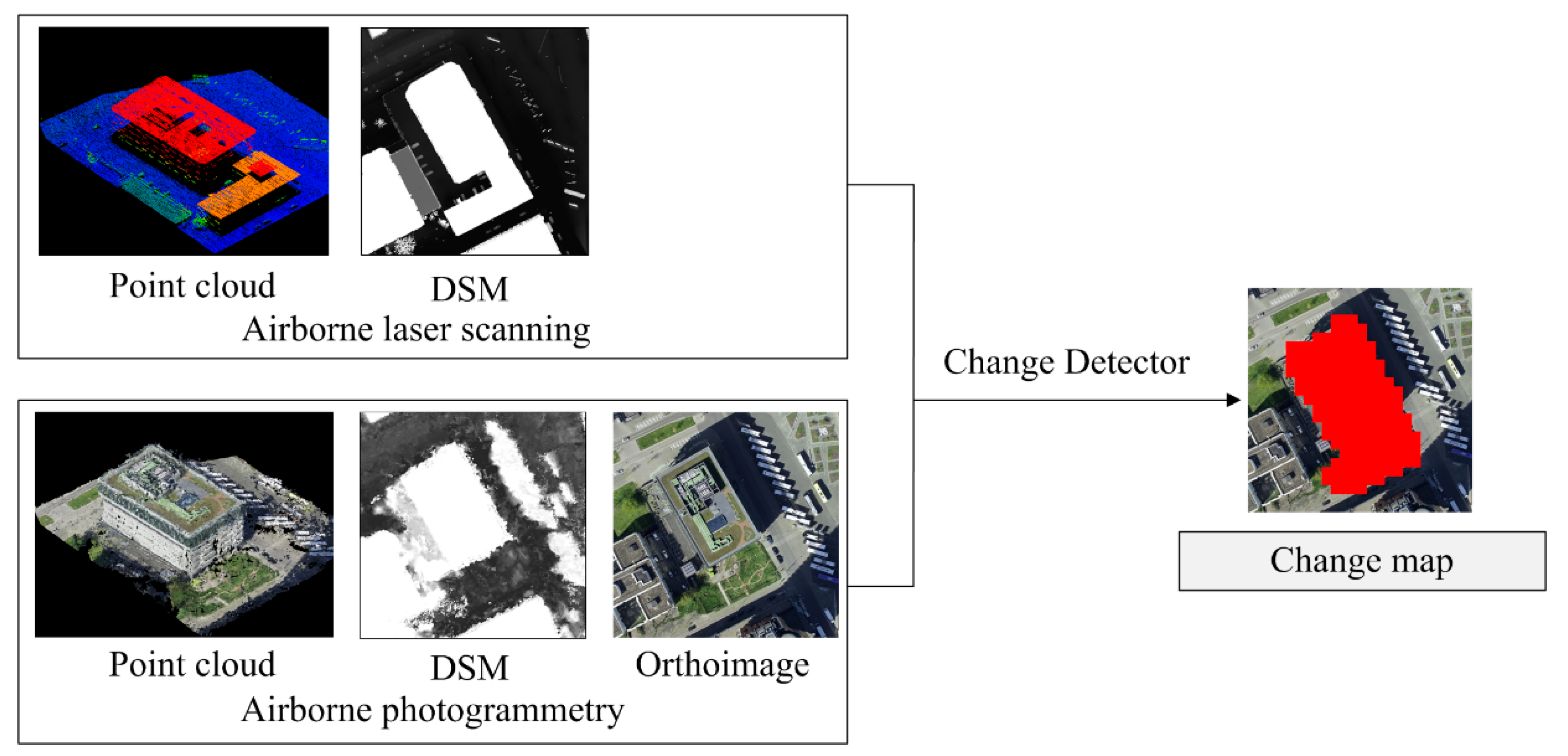
  • We propose a method to detect building changes between ALS data and photogrammetric data. First, we provide an effective solution to convert and normalize multimodal point clouds to 2D image patches. The converted image patches are fed into a lightweight pseudo-Siamese convolutional neural network (PSI-CNN) to quickly detect change locations.
  • The proposed PSI-CNN is compared to five other CNN variants with different inputs and configurations. In particular, the performance of the pseudo-Siamese architecture and feed-forward architecture are compared quantitatively and qualitatively. Different configurations of multimodal inputs are compared.
This paper is organized as follows: Section 2 reviews the related work. Section 3 presents the methods. Section 4 provides details on the study area and experimental settings. Section 5 presents the results and analyses. Section 6 concludes the paper.

2. Related Work

2.1. Multimodal Change Detection

Change detection is the process of identifying differences in an object by analyzing it at different epochs [12]. The input data of two epochs can be either raw remote sensing data or object information from an existing database. Change detection can be performed either between 3D data or by comparing 3D data of a single epoch to a bi-dimensional map [13]. Zhan et al. [14] classified the change detection methods into two categories based on the workflow: Post-classification comparison (e.g., [15,16]) and change vector analysis (e.g., [17,18,19]).
In post-classification comparison, independent classification maps are required for both epochs. Change detection is then performed by comparing the response at the same location between the two epochs. When the data of two epochs are of different modalities, both training and testing have to be performed at each epoch separately, thus requiring a large computational effort. Moreover, errors tend to be multiplied along object borders due to misclassification errors in the single classification maps [20]. Vosselman et al., [13] proposed a method to update 2D topographical maps with laser scanning data. The ALS data were first segmented and classified. The building segments were then matched against the building objects of the maps to detect the building changes. Malpica et al. [21] detected building changes in a vector geospatial database. The building objects were extracted from satellite imagery and laser data using a support vector machine (SVM).
In contrast, change vector analysis relies on extracting comparative change vectors between the two epochs and fuses the change indicators in the final stage [22,23]. Compared with post-classification comparison, change vector analysis directly makes a comparison between the data of both epochs. However, traditional change vector analysis is sensitive to data problems and usually causes many false detections, especially when the data of two epochs are in different modalities. The most widely-used change vector analysis between 3D data sets is DSM surface differencing, followed by point-to-point or point-to-mesh comparison [5,8]. To reduce the number of false positives, direct comparison methods are often followed by post-processing methods or are combined with other change detection frameworks.
Considering detecting changes between multimodal 3D data, Basgall et al. [24] compared laser points and dense matching points with the CloudCompare software. Their study area was small and only one changed building was studied. Also, the method proposed was not automatic, since the changed building was detected through visual inspection. Qin and Gruen [3] detected changes between mobile laser points and terrestrial images at street level. Image-derived point clouds were projected to each image by a weighted window-based Z-buffering method. Then over-segmentation-based graph cut optimization was carried out to compute the changed area in the image space. Evaluation results showed that 81.6% changed pixels were correctly detected. Du et al. [25] detected building changes in outdated dense matching point clouds using new laser points, which is the reverse setup compared with our work. Height difference and gray-scale dissimilarity were used with contextual information to detect changes in the point cloud space. Finally, the preliminary changes were refined based on handcrafted features. The limitation of the approach raised by the authors was that the boundary of changed buildings could not be determined accurately. Additionally, the method required human intervention and prior knowledge in multiple steps. By contrast, our method aims at a method for multimodal change detection, which requires minimal human intervention and generates reliable change locations.

2.2. Deep Learning for Multimodal Data Processing

Recently, deep CNNs have demonstrated their superior performance in extracting representative features for various computer vision tasks (e.g., image classification, semantic segmentation, and object detection [26,27,28]). As a specific CNN architecture, Siamese networks (SI-CNN) perform well in applications which compute similarity or to detect changes between two inputs. Outputs from SI-CNNs can be patch-based single-valued or dense pixel-by-pixel maps, depending on the specific architecture. In patch-based prediction, SI-CNN has been widely used in handwritten digit verification [29], face verification [30,31], character recognition [32], patch-based matching [33], and RGB-D object recognition [34]. In the case of dense predictions, the SI-CNN was used in wide-baseline stereo matching [35,36].
In the remote sensing domain, deep learning has also been used to process two sets of input in change detection and image matching. He et al. [37] used a SI-CNN to find corresponding satellite images with complex background variations. The coordinates of the matching points were searched using a Harris operator followed by a quadratic polynomial constraint to remove false matches. Similarly, Lefèvre et al. [38] used a SI-CNN to detect changes between aerial images and street level panoramas reprojected on an aerial perspective. AlexNet [39] was used in the two branches for feature extraction and the Euclidean distance was used to determine the similarity between the two views. Mou et al. [40] identified corresponding patches between SAR images and optical images using a pseudo SI-CNN (pseudo indicates that the weights in the two branches are unshared). The weights in the two branches are unshared so that different parameters are applied to extract features from multimodal inputs. The feature maps from the two Siamese branches were concatenated, which worked as a patch comparison unit. Although SAR images and aerial images involved heterogeneous properties, they achieved an overall accuracy of 97.48%.
Some recent studies obtained dense per-pixel change maps by using a Siamese fully convolutional neural network (FCN). Zhan et al. [14] maintained the original input size in each convolutional layer in the two branches followed by a weighted contrastive loss function. The pixels with a distance measure higher than a given threshold were regarded as changed. The acquired change maps were then post-processed by the K-nearest neighbor approach. Daudt et al. [41] adopted a different architecture combined with convolutional blocks and transpose convolution blocks to output full change maps between satellite images. Mou et al. [16] proposed to learn spectral-spatial-temporal features using a recurrent neural network (RNN) for change detection in multispectral images. This end-to-end architecture can adaptively learn the temporal dependence between multi-temporal images. In our work, we also propose a light-weighted SI-CNN for change detection.

3. Materials and Methods

A building is defined as changed in two situations: (1) it is a building in one epoch but not in the other epoch (i.e., the building is newly-built or demolished); (2) a building exists in two epochs but has changed in height or extent. In both situations, our method aims at detecting the change locations using a light-weighted SI-CNN. First, the multimodal input data are converted and normalized to the same range [ 0 ,   1 ] ; Then the normalized data are fed into an SI-CNN for change detection. The inputs and output of our method are shown in Figure 2. The old epoch contains an ALS point cloud and the derived DSM; the new epoch contains a DIM point cloud, DSM, and orthoimage. The output is the change map which indicates the change locations.

3.1. Preprocessing: Registration, Conversion, and Normalization

First, the point clouds from two epochs and orthoimages from the second epoch are converted to the same resolution and the same coordinate system. The products from the photogrammetric workflow are geo-referenced to the world coordinate systems using ground control points (GCPs) during bundle adjustment. The accuracy of the dense matching points, DSMs, and orthoimages are affected by the accuracy of the interior and exterior orientation elements. The coordinates of the airborne laser points are already provided in the same world coordinate system.
Second, the laser points are converted to DSMs (ALS-DSM) using LAStools. The photogrammetric DSMs (DIM-DSMs) and orthoimages are generated from a photogrammetric workflow. The ALS-DSM and DIM-DSM are resampled so that their grid coordinates are strictly alighted with the pixels on the orthoimage.
Next, the heights of ALS-DSM and DIM-DSM are normalized to the same height range. The two DSMs range in [ H m i n ,   H m a x ] where H m i n and H m a x are the minimum and maximum DSM height of the whole study area, respectively. We normalize the height values ( H 0 ) of the ALS-DSM and DIM-DSM using the same H m i n and H m a x as shown in Equation (1). In this way, the two DSMs are converted to the range of [ 0 ,   1 ] . This representation approach maintains all the height details in the DSM.
H = ( H 0 H m i n ) / ( H m a x H m i n )
In addition, the three channels R, G, and B of the orthoimages from dense matching are also normalized to [ 0 ,   1 ] by simply dividing each pixel value by 255. Hence, all the five channels ALS-DSM, DIM-DSM, R, G and B are normalized within the [ 0 , 1 ] range. Image patches are then cropped in the overlapping raster images for the pseudo-Siamese network.

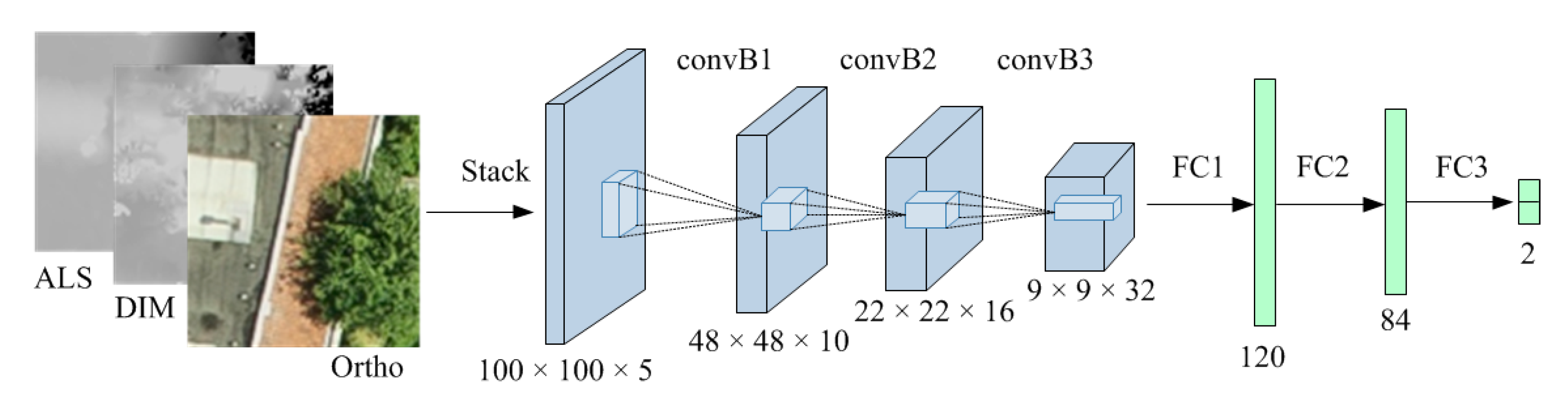
3.2. Network Architecture

The registered three patches (ALS-DSM, DIM-DSM, and orthoimage) including five channels (ALS-DSM, DIM-DSM and R, G, B) are fed into the SI-CNN for change detection. The proposed SI-CNN model is called PSI-DC (i.e., pseudo-Siamese-DiffDSM-Color) (see Figure 3). DiffDSM refers to the height difference between the ALS-DSM and DIM-DSM. The input for this branch is one channel. For the other branch, the R, G, B channels from the orthoimage patch are provided. Our preliminary tests show that a Siamese CNN has difficulties converging when the data modalities in a given branch are heterogeneous. Thus, we do not present the architecture with the ALS-DSM as the first branch and DIM-DSM and R, G, B as the other, as a traditional Siamese network is designed. Instead, we pass a different DSM in the first branch and the color information from the R, G, B bands from the orthoimages in the other.
In Figure 3, the inputs are processed by three convolutional blocks (convB) consecutively. The extracted feature maps are concatenated and further processed by one convB and three fully connected (FC) layers. Each convolutional block contains a convolution operation followed by a rectified linear unit (ReLU) as the activation function. Further, convB1, convB2, and convB4 also contain a max-pooling layer which adds translation invariance to the model and decreases the number of parameters to learn [42]. The size of the convolution kernels is 5 × 5 in our network, with a padding size of 0 and slide of 1, which is verified to be an effective compromise between the feature extraction depth and contextual extent in our task.
Our network is conceptually similar to the change detection network proposed by [40], which has eight convolutional blocks for feature extraction and two blocks after concatenation. In their work, the two patches to be compared are not only from different sensors (SAR and optical), but also involve translation, rotation, and scale changes. Our case is simpler since our compared patches are strictly registered and normalized to the same scale. Therefore, we use fewer convolution blocks to extract features from multimodal data.
Fully connected layers are used in the final stages of the network for high-level reasoning. PSI-DC contains three FC layers. The first two FC layers are followed by ReLU operations. The last FC layer outputs a 2 × 1 vector, which indicates the probability for changed and unchanged, respectively. In this way, we convert a change detection task into a binary classification task. Suppose that ( x 1 , x 2 ) is the 2 × 1 vector predicted from the last FC layer, the loss is computed between ( x 1 , x 2 ) and the ground truth (1 for changed and 0 for unchanged). First, the vector is normalized to ( 0 ,   1 ) by a Softmax function:
p i = exp ( x i ) exp ( x 1 ) + exp ( x 2 )   ,   i = 1 , 2
where p 1 + p 2 = 1 . Then, a weighted binary cross entropy loss is calculated:
L o s s = ( w 1 y log ( p 1 ) + w 2 ( 1 y ) log ( p 2 )
where y is the reference label and p i is the predicted logit from the Softmax function. The ratio of w 1 to w 2 is set based on the number of negative training samples and positive samples. In urban scenes, the number of negative samples (unchanged) is usually several times the number of positive samples (changed). By assigning weights to the loss function, we provide a larger penalization to a false positive than to a false negative to suppress false positives.

4. Experiments

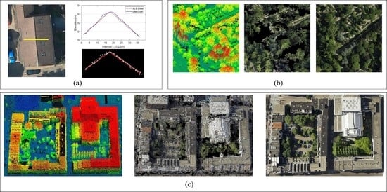
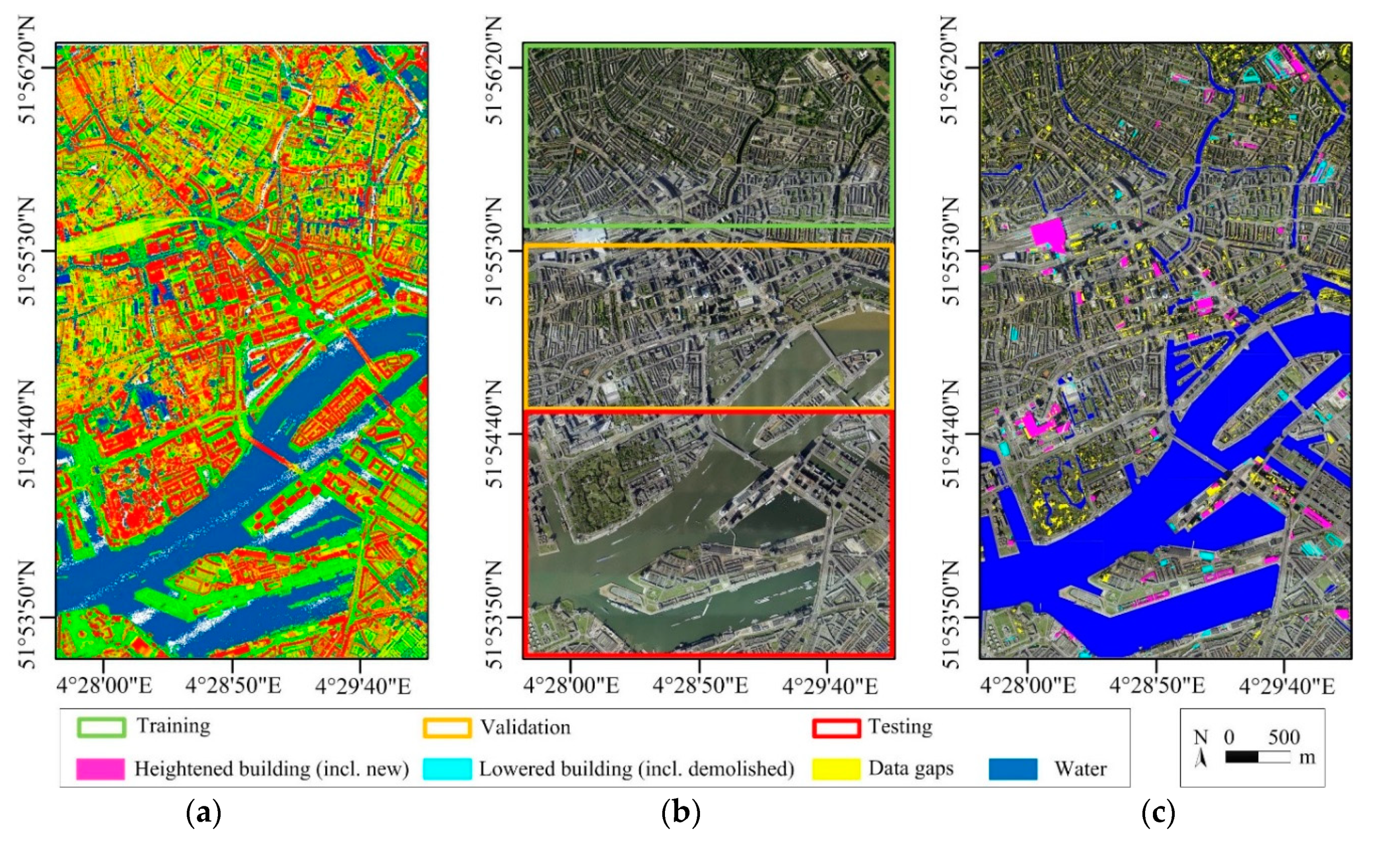
4.1. Descriptions of Experimental Data

The study area is located in Rotterdam, The Netherlands, which is a densely built port city mainly covered by residential buildings, skyscrapers, vegetation, roads, and waters. The study area is 14.5 km2 as shown in Figure 4. Figure 4a shows the ALS point cloud obtained in 2007 with a density of approximately 25 points/m2. The point cloud contains approximately 226 million points.
A total of 2160 aerial images were obtained by CycloMedia [43] from five perspectives in 2016. The flying altitude was approximately 450 m. The tilt angle of the oblique view was approximately 45°. The image size was 7360 × 4912 pixels. The GSD of nadir images equaled 0.1 m. The bundle adjustment and dense image matching were performed in Pix4Dmapper. The vertical RMSE (Root Mean Square Error) of 48 GCPs was ±0.021 m and the vertical RMSE of 20 check points was ±0.058 m. The overlap of nadir images was approximately 80% along the track and 40% across the track. Even though the overlap rate from five views is high, dense matching still cannot perform well in the narrow alleys between tall buildings due to occlusion, poor illumination, and image contrast. The DIM point cloud contains approximately 281 million points. DSMs and orthoimages were also generated at the same resolution of 0.1 m. Figure 4b shows the generated orthoimage. The training, validation, and testing area make up 28%, 25%, and 42% of the study area, respectively. Note that 5% of the block (between training and validation area) is not used since this area contains the newly-built Rotterdam railway station with homogeneous building change; the samples extracted from this area will reduce the sample diversity and may lead to under-fitted CNN models. Figure 4c shows the orthoimage overlaid with four types of labels: Heightened building, lowered building, water, and data gaps.

4.2. Experimental Setup
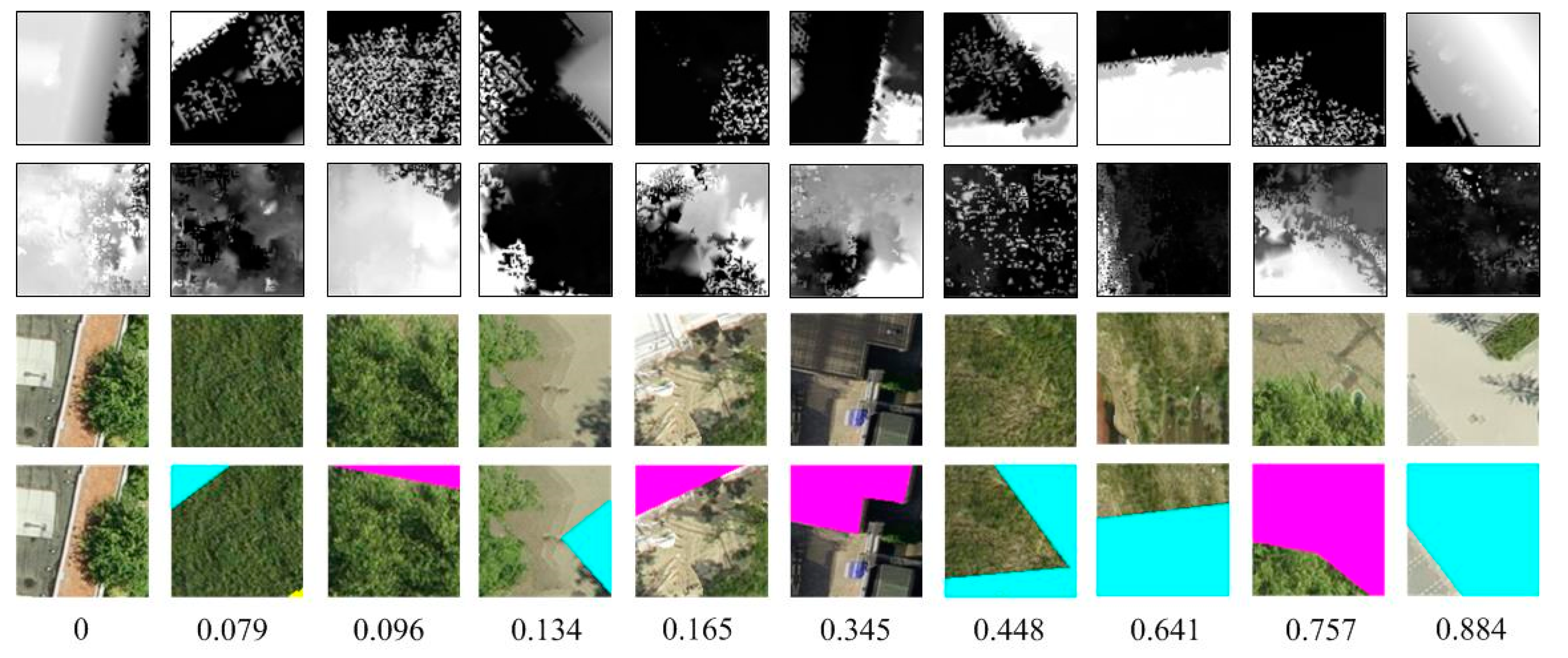
After data pre-processing, the grid coordinates of the ALS-DSM and DIM-DSM are registered with the pixels in orthoimages at a GSD of 0.1 m. When extracting samples for PSI-DC, each sample contains one ALS-DSM patch, one DIM-DSM patch, and one orthoimage patch. The patch size is 100 × 100 pixels, which corresponds to 10 m × 10 m on the ground.
Before extracting patches from the normalized ALS-DSM, DIM-DSM, and orthoimage, the ground truth for building changes should be prepared. The building changes are manually labeled on the orthoimage with guidance of the ALS point, DIM points, and DSM differencing map. Concretely, when a building is newly-built or heightened on the DIM data, the boundary is delineated from the DIM point clouds; when a building is demolished or lowered, its boundary is delineated from the outdated ALS point cloud. In addition, data gaps and water are marked on the ground truth map, but they are not considered for change detection. Data gaps may appear in ALS points and/or DIM points. If there is no data in either epoch, we simply cannot make any inference whether it is changed or not; thus, we label the ground truth map as “data gap”. We also ignore water height changes caused by tides. Finally, each pixel on the ground truth map is labeled as changed building, data gap, water, or other. Specifically, the changed building class includes heightened (including newly-built) and lowered (including demolished) buildings. The other class includes all the irrelevant changes and unchanged areas.
Then small square patches are cropped from the raster images densely with a given overlap. A critical question is how to define a changed patch and an unchanged patch. Some previous patch-based classification work assigned the label of the central pixel of a patch to the whole patch [44,45]. However, this definition method is sensitive to slight displacements of the patch location. In this paper, we label the patch as changed if the ratio of changed pixels in this patch is larger than a threshold. The rules used for patch labeling are as follows:
(1)
If the ratio of pixels for water and data gaps is larger than T P S 1 then eliminate this patch.
(2)
If the ratio of changed pixels is larger than T P S 2 this patch is labeled as changed; otherwise it is unchanged.
The settings and descriptions of parameters are listed in Table 1. Among them, T H d and T l e n g t h are set according to the DIM data quality. T P S 1 and T P S 2 are set based on trial experiments.
Since the training area contains far fewer changed (positive) samples than unchanged (negative) samples, two strategies were adopted when preparing changed training samples: (1) half-overlap sampling involves electing positive patches with a stride of half-patch size (i.e., 5 m) which makes complete sampling of the changed areas as shown in Figure 5; (2) data augmentation requires that each positive sample, including three patches, is horizontally and vertically flipped and also rotated by 90°, 180°, and 270° [14]. When preparing negative training samples, validation samples, and testing samples, half-overlap sampling is adopted but data augmentation is not.
The number of training, validation, and testing samples is shown in Table 2. Since variable amounts of building construction work has happened in different areas, the ratios of changed-to-unchanged samples in the training, validation, and testing areas are quite different. The ratio w 1 : w 2 in Equation (3) is set to the reciprocal of this changed-to-unchanged ratio in the training set.
Figure 6 shows three negative and seven positive training samples. The ratio of changed pixels varies from low to high from left to right. Note that the first sample in Figure 6 contains a new tree in the DIM data. Our CNN model should be trained to distinguish a relevant building change from an irrelevant tree change. In addition, our definition of a changed patch is based on the ratio of changed pixels rather than the label of the central pixel. The center of the seventh sample in Figure 6 is unchanged, but we define it as changed since 44.8% of pixels are changed. This rule for defining changed patches is more inclusive of the ensemble of the content of the patch than labeling a patch according to the central pixel, which is supposed to be easier for a CNN to learn.
When training networks, weights are randomly initialized, and all networks are trained from scratch. The weights in the two Siamese branches were not shared, since the inputs involved heterogeneous properties. The batch size was 128. The optimization algorithm was a stochastic gradient descent (SGD) with momentum [42]. The learning rate started from 0.008 and decreased by 0.003 after every 30 epochs. We trained the network for 80 epochs with a momentum of 0.90. The training process was run on a single NVIDIA GeForce GTX Titan GPU with 11G memory. The CNN architectures were implemented in PyTorch [46].

4.3. Contrast Experiments

For the CNN architecture, apart from the proposed PSI-DC architecture, five other architectures were implemented as our baseline methods to compare the performance of different CNN configurations: PSI-HHC (height–height–color), PSI-HH (height–height), feed-forward (FF)-HHC, FF-DC, FF-HH. In addition, a simple DSM differencing method was also implemented as a baseline method. The details of these methods are listed below:
  • PSI-HHC: The proposed PSI-DC directly took the difference between the two DSMs in the beginning. We also implemented an architecture which uses the ALS-DSM and DIM-DSM together as one branch (two channels) and takes R, G, B as the other branch (three channels). This architecture called PSI-HHC works as a late fusion of the two DSMs, compared with PSI-DC.
  • PSI-HH: In this SI-CNN architecture, one branch is the ALS-DSM and the other is the DIM-DSM. Color channels are not applied.
  • FF-HHC: It is interesting to compare the performance of feed-forward architecture and pseudo-Siamese architecture for our task. A feed-forward CNN (FF-HHC) is adopted as shown in Figure 7. The five channels are stacked in the beginning and then fed into convolutional blocks and fully connected layers for feature extraction. HHC (height–height–color) indicates that two DSM patches and one orthoimage patch are taken as input. For more details, the readers are referred to [47].
  • FF-DC: This feed-forward architecture takes four channels as input: DiffDSM, R, G, and B.
  • FF-HH: This feed-forward architecture takes the ALS-DSM and DIM-DSM as input. Color channels are not applied.
  • DSM-Diff: Given two DSM patches from ALS data and DIM data over the sample area, a simple DSM differencing produces differential-DSM. The height difference averaged over each pixel on the patch will bring the average height difference (AHD) between the two patches. Intuitively, the two patches are more likely to be changed if the AHD is high, and vice versa. The optimal AHD threshold can be obtained with Otsu’s thresholding algorithm [48]. This method can classify the patches into changed or unchanged in an unsupervised way.

4.4. Evaluation Metrics

Our change detection results are evaluated at the patch-level. Recall, precision and F1-score are applied to evaluate this strongly-imbalanced binary classification problem. Recall indicates the ability of a model to detect all the real changes. Precision indicates the ratio of true changes among all the detected changes. The F1-score is a metric to combine recall and precision using their harmonic mean.
R e c a l l = T P / ( T P + F N )
P r e c i s i o n = T P / ( T P + F P )
F 1 = 2 × ( R e c a l l × P r e c i s i o n ) / ( R e c a l l + P r e c i s i o n )
True positive (TP) is the number of correctly detected changes. True negative (TN) is the number of unchanged samples detected as unchanged. False positive (FP) is the number of changes detected by the algorithm, which are not changes in the real scene. False negative (FN) is the number of undetected changes.

5. Results and Discussion
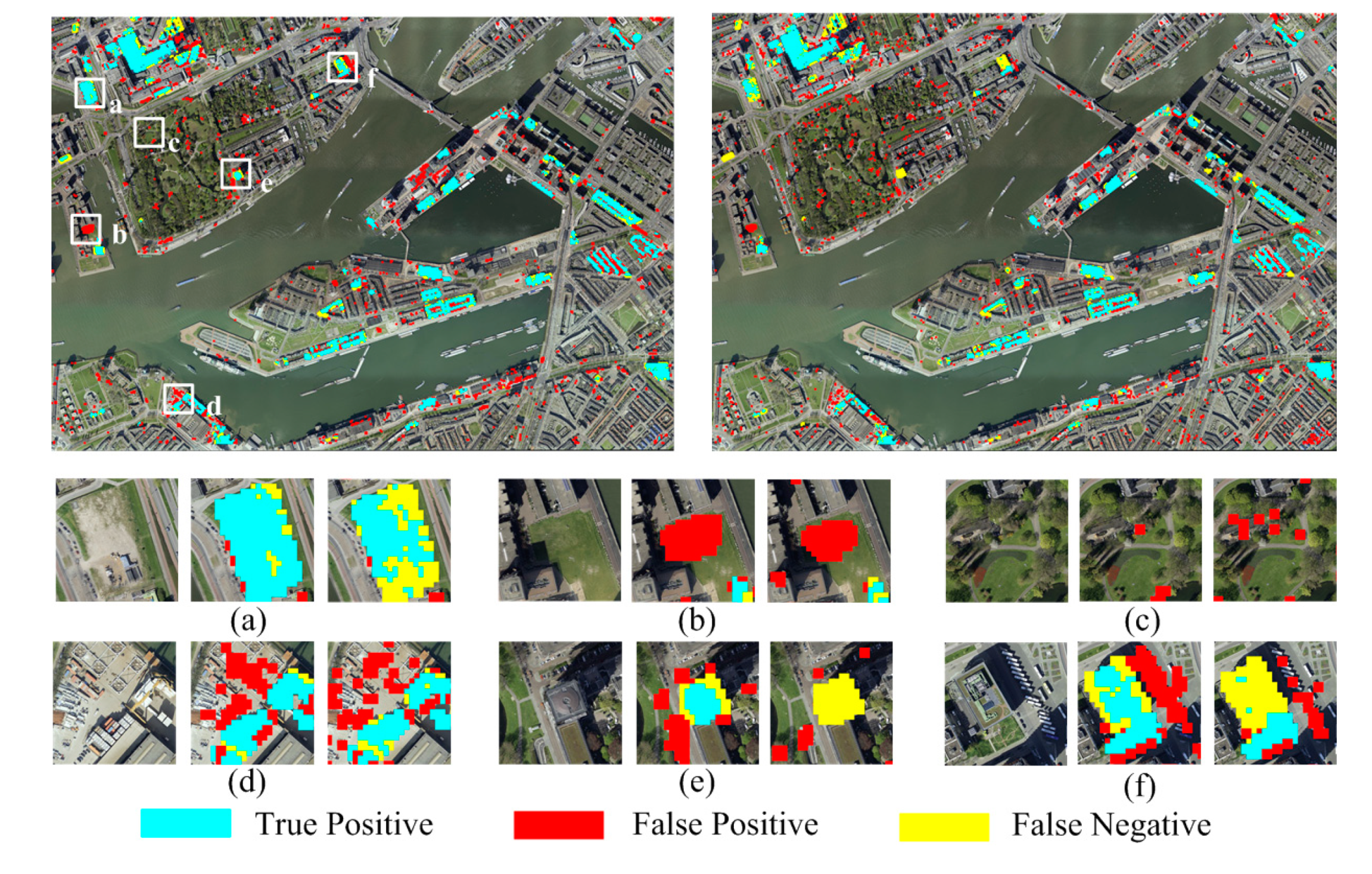
5.1. Results

During training, the CNN model was evaluated on the validation set after every three epochs to check its performance and ensure that there was no overfitting. Towards the end of training, the model with the highest F1-score was selected as the final trained model. The validation results of the proposed PSI-DC are as follows: TP was 2362; TN was 101,636; FP was 2475; FN was 563. Recall equaled 80.75%; precision equaled 48.83%; F1-score equaled 60.86%. That is, 80.75% of positive samples were correctly inferred as positive and 97.62% of negative samples were correctly inferred as negative. The patch-level change detection results on the test set from the three CNN architectures are shown in Table 3.
Table 3 shows that the proposed PSI-DC model outperforms the other six methods in precision and F1-score. The recall of PSI-DC ranks the second among the seven methods and is better than the other five CNN-based methods. The F1-score of FF-HHC ranks second among the seven. The recall of FF-HHC is lower than PSI-DC by 4%, and its precision is lower than the latter by 0.99%, which results into a F1-score of 73.92%. The lowest F1-score is obtained by DSM-Diff, which is lower than the second lowest F1-score by a large margin (17.37%). The recall of DSM-Diff (89.12%) is the highest among the seven, while its precision is merely 37.61% (i.e., DSM-Diff misclassifies many unchanged patches into changed, which results into many false positives). The poor result of DSM-Diff indicates that the AHD threshold (3.82 m) found by Otsu’s method cannot distinguish between unchanged and changed patches effectively. The reason is that many unchanged patches also present a high AHD value (e.g., patches on the vegetated land or under shadow). A single AHD threshold cannot make a correct distinction.
Comparing Siamese architecture and feed-forward architecture, the results of FF-HH and PSI-HH show a margin in F1-score of only 0.54%, which indicates that the performance of feed-forward and Siamese architectures differ very slightly when the input contains only the ALS-DSM and DIM-DSM. However, the F1-score of FF-HHC is higher than that of PSI-HHC by 3%. In this case, the feed-forwards architecture performs better than the Siamese model. This can be explained by the fact that PSI-HHC contains two branches and FF-HHC contains only one branch. PSI-HHC is more complicated and contains more parameters, which might be harder to train.
Concerning the impact of color channels, FF-HHC outperforms FF-HH and PSI-HHC outperforms PSI-HH. This clearly demonstrates that color channels from orthoimage contribute to the correct classification of unchanged and changed patches. The spectral and textural features derived from orthoimage is supplementary to the geometric features derived from two DSMs.
Comparing different input configurations (DC vs. HHC), PSI-DC performs better than PSI-HHC by a large margin of 5.21% in the F1-score. This large margin indicates that the input configuration to the CNN models has a significant impact on the change detection results. The PSI-DC and PSI-HHC networks are all the same except that one branch in PSI-DC is Diff-DSM while the same branch is replaced by raw ALS-DSM and DIM-DSM patches in PSI-HHC. This is because PSI-DC takes advanced features (height difference of two DSMs) as input, while PSI-HHC takes two raw DSMs as input. PSI-HHC has more parameters and requires the CNN model to learn deeper. However, in the feed-forward model, FF-DC performs slightly worse than FF-HHC by 1.22%, which is against our finding in comparison between PSI-HHC and PSI-DC. A sound explanation is that there are much less parameters in the feed-forward model than in the Siamese model. When the two raw DSMs are taken as inputs in the FF-HHC, FF-HHC can learn more geometric features from the two raw DSMs other than differential DSM features, which results in a better classification result.
The change maps generated from PSI-DC and FF-HHC (i.e., two optimal models) are visualized in Figure 8. For other qualitative results from feed-forward models, the readers can refer to [47]. Figure 8 shows that most changed objects are correctly detected in the patch-level results even though some false detections occur. Although the patch-level change masks show a zigzag effect, the results still reflect coarse locations of the change boundaries. The six examples in the lower part of Figure 8 visualize some details of the change maps. Figure 8a shows a demolished factory. The patch-based change map from PSI-DC can represent the boundary much better than FF-HHC since many false negatives (i.e., omission errors) appear in the latter. Figure 8b shows that a deep pit in a construction site is misclassified into a changed building by both models. Figure 8c shows that more false positives appear in the vegetation area from the model FF-HHC than in the prediction of PSI-DC. This area is located in a park covered with grassland, trees, rivers, and dirt roads. The point cloud from dense matching contains much noise in this area. PSI-DC can better classify this area into non-changes than FF-HHC. Figure 8d shows another construction site at the port. Tall tower cranes, containers, and trucks are misclassified into building-related changes because their heights and surface attributes are similar to a real building. Figure 8e shows that a heightened square building is omitted by FF-HHC while it is detected by PSI-DC. Figure 8f shows that FF-HHC makes more false negatives than PSI-DC, even though FF-HHC causes less false positives than PSI-DC.

5.2. Visualization of Feature Maps

In order to understand what the CNN learns, the feature maps from the last convB in PSI-DC are visualized in Figure 9. The outputs of PSI-DC are 64 7 × 7 feature maps. Only the strongest half of the feature maps are shown. Two samples are visualized including a new building and a demolished building. The activation is dispersed in multiple feature maps. In some of the feature maps, the direction and shape of the activation reflect the shape of the change (e.g., the 25th feature map in Figure 9a and the 8th, 9th, 16th, and 32nd feature maps in Figure 9b, which are highlighted in red frames. The activations from the last convB are then flattened and summed up in the fully connected layers, which matches with our definition of changed patches. Namely, whether a patch is changed or not depends on the ratio of changed pixels, rather than merely the central pixel.

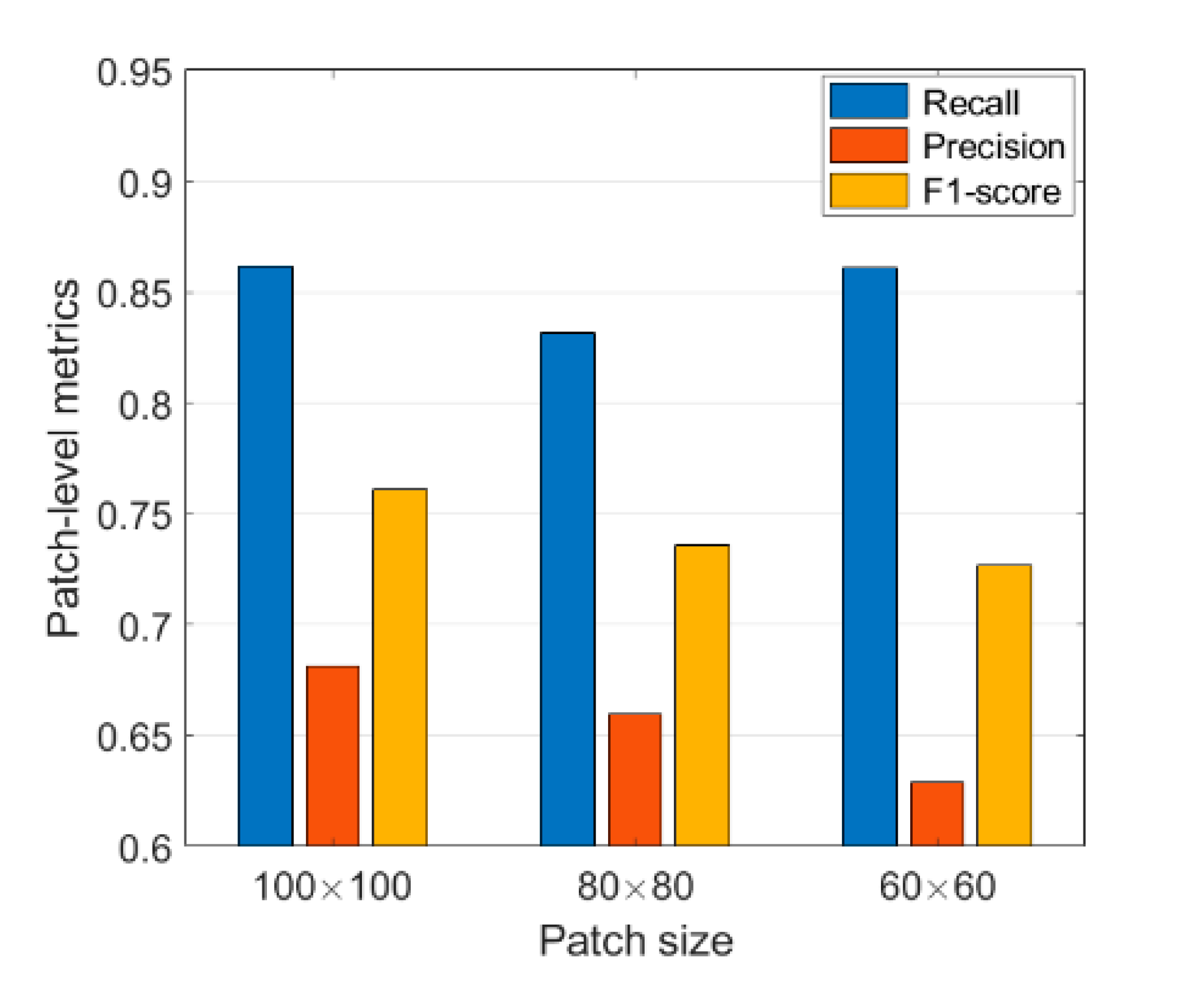
5.3. Impact of Patch Size

Patch size is a critical hyper-parameter in our framework. It should be large enough to incorporate much contextual information for patch-based change detection. It should be small enough to guarantee a relatively detailed and accurate localization of changed buildings. We make comparative studies by selecting samples with sizes of 80 × 80 and 60 × 60 from the converted DSMs and orthoimages, and then run the whole workflow from scratch. To make the comparison meaningful, we maintain the original PSI-DC architecture but up-sample the three patches (ALS-DSM, DIM-DSM, and orthoimage) to 100 × 100 to fit the CNN inputs. In addition, the numbers of positive and negative training samples in 80 × 80 and 60 × 60 tests are all the same with those in the 100 × 100 test. When extracting samples from the testing area, the number of samples for 80 × 80 and 60 × 60 tests is 1.6 times and 2.9 times of the number in the 100 × 100 test, respectively.
Figure 10 shows the impact of patch size on the patch-level change maps. Both the precision and F1-score show a clear decreasing trend when the patch size decreases, even though the recall shows some fluctuation. This can be explained by the fact that the precision decreases when less contextual information is contained in the smaller patches.

6. Conclusions

We propose a method to detect building changes between airborne laser scanning and photogrammetric data. This task is challenging owing to the multi-modality of input data and dense matching errors. The multimodal data are converted to the same scales and fed into a lightweight pseudo-Siamese CNN for change detection. Our results show that our change map achieves a recall rate of 86.17%, a precision rate of 68.16%, and an F1-score of 76.13%. Although the point cloud quality from dense matching is not as good as laser scanning points, the radiometric and textural information provided by the orthoimages serves as a supplement, which leads to relatively satisfactory change delineation results. The advantages with the design of our method are as follows: Firstly, the complicated multimodal change detection problem is transformed into a binary classification problem which is solved by one CNN, which requires less hyper-parameters and prior knowledge compared to previous methods (e.g., [11,25]). The PSI-DC model is lightweight but works satisfactorily for the problem at hand. Secondly, the change detection module based on a pseudo-Siamese CNN can quickly provide some initial change maps in emergency response.
This paper also compares the proposed PSI-DC model with five other CNN models and one naive change detection method based on surface differencing. The six CNN models present different input configurations or network architectures. We conclude that spectral and textural features provided by orthoimage contribute to the classification performance. Siamese architecture is preferred over the feed-forward model when the inputs are in different modalities. However, it should be noted that a Siamese CNN might contain more parameters and is harder to train.
In future work, the multimodal change detection work can be extended in three aspects. First, dense image matching takes a lot of effort. It would be more efficient if the aerial images were compared to the ALS point cloud directly for change detection. Second, fully convolutional networks may also be considered for per-pixel change detection, since they add more contextual features. It is worthy of researching end-to-end FCN-based change detection methods without using any post-processing [14]. Finally, end-to-end change detection between multi-epoch 3D point clouds without converting to 2D raster images may also be feasible, owing to the recent advances in 3D CNNs.

Author Contributions

Z.Z.; M.Y.Y.; and G.V. designed and implemented the experiments. M.G. contributed to processing of the data. C.P. and D.T. contributed to the analysis and interpretation of the results. The manuscript was written by Z.Z. with contributions from all the other co-authors.

Funding

This research was funded by the China Scholarship Council (CSC).

Acknowledgments

The data is provided by CycloMedia. The authors gratefully acknowledge the support. The authors also acknowledge NVIDIA Corporation for the donated GPUs.

Conflicts of Interest

The authors declare no conflicts of interest.

References

  1. Tran, T.H.G.; Ressl, C.; Pfeifer, N. Integrated change detection and classification in urban areas based on airborne laser scanning point clouds. Sensors 2018, 18, 448. [Google Scholar] [CrossRef] [PubMed]
  2. Matikainen, L.; Hyyppä, J.; Kaartinen, H. Automatic detection of changes from laser scanner and aerial image data for updating building maps. Int. Arch. Photogramm. Remote Sens. Spat. Inf. Sci. 2004, 35, 434–439. [Google Scholar]
  3. Qin, R.; Gruen, A. 3D change detection at street level using mobile laser scanning point clouds and terrestrial images. ISPRS J. Photogramm. Remote Sens. 2014, 90, 23–35. [Google Scholar] [CrossRef]
  4. Zhang, Z.; Gerke, M.; Vosselman, G.; Yang, M.Y. A patch-based method for the evaluation of dense image matching quality. Int. J. Appl. Earth Obs. Geoinf. 2018, 70, 25–34. [Google Scholar] [CrossRef]
  5. Remondino, F.; Spera, M.G.; Nocerino, E.; Menna, F.; Nex, F. State of the art in high density image matching. Photogramm. Rec. 2014, 29, 144–166. [Google Scholar] [CrossRef] [Green Version]
  6. Nex, F.; Gerke, M.; Remondino, F.; Przybilla, H.J.; Bäumker, M.; Zurhorst, A. ISPRS benchmark for multi-platform photogrammetry. ISPRS Ann. Photogramm. Remote Sens. Spat. Inf. Sci. 2015, 2, 135–142. [Google Scholar] [CrossRef]
  7. Ressl, C.; Brockmann, H.; Mandlburger, G.; Pfeifer, N. Dense image matching vs. airborne laser scanning–comparison of two methods for deriving terrain models. Photogramm. Fernerkund. Geoinf. 2016, 2, 57–73. [Google Scholar] [CrossRef]
  8. Mandlburger, G.; Wenzel, K.; Spitzer, A.; Haala, N.; Glira, P.; Pfeifer, N. Improved topographic models via concurrent airborne lidar and dense image matching. ISPRS Ann. Photogram. Remote Sens. Spat. Inf. Sci. 2017, IV-2/W4, 259–266. [Google Scholar] [CrossRef]
  9. Hirschmüller, H. Stereo processing by semi-global matching and mutual information. IEEE Trans. Pattern Anal. Mach. Intell. 2008, 30, 328–341. [Google Scholar] [CrossRef]
  10. Rothermel, M.; Wenzel, K.; Fritsch, D.; Haala, N. SURE: Photogrammetric surface reconstruction from imagery. In Proceedings of the LC3D Workshop, Berlin, Germany, December 2012; Volume 8, p. 2. [Google Scholar]
  11. Xu, S.; Vosselman, G.; Oude Elberink, S. Detection and classification of changes in buildings from airborne laser scanning data. Remote Sens. 2015, 7, 17051–17076. [Google Scholar] [CrossRef]
  12. Singh, A. Digital change detection techniques using remotely-sensed data. Int. J. Remote Sens. 1989, 10, 989–1003. [Google Scholar] [CrossRef]
  13. Vosselman, G.; Gorte, B.G.H.; Sithole, G. Change detection for updating medium scale maps using laser altimetry. Int. Arch. Photogramm. Remote Sens. Spat. Inf. Sci. 2004, 34, 207–212. [Google Scholar]
  14. Zhan, Y.; Fu, K.; Yan, M.; Sun, X.; Wang, H.; Qiu, X. Change detection based on deep Siamese Convolutional Network for optical aerial images. IEEE Geosci. Remote Sens. Lett. 2017, 14, 1845–1849. [Google Scholar] [CrossRef]
  15. Wu, C.; Du, B.; Cui, X.; Zhang, L. A post-classification change detection method based on iterative slow feature analysis and Bayesian soft fusion. Remote Sens. Environ. 2017, 199, 241–255. [Google Scholar] [CrossRef]
  16. Mou, L.; Bruzzone, L.; Zhu, X.X. Learning spectral-spatial-temporal features via a recurrent convolutional neural network for change detection in multispectral imagery. IEEE Trans. Geosci. Remote Sens. 2019, 57, 924–935. [Google Scholar] [CrossRef]
  17. Choi, K.; Lee, I.; Kim, S. A feature based approach to automatic change detection from LiDAR data in urban areas. Int. Arch. Photogramm. Remote Sens. Spat. Inf. Sci. 2009, 18, 259–264. [Google Scholar]
  18. Volpi, M.; Camps-Valls, G.; Tuia, D. Spectral alignment of multi-temporal cross-sensor images with automated kernel canonical correlation analysis. ISPRS J. Photogramm. Remote Sens. 2015, 107, 50–63. [Google Scholar] [CrossRef]
  19. Gong, M.; Zhan, T.; Zhang, P.; Miao, Q. Superpixel-based difference representation learning for change detection in multispectral remote sensing images. IEEE Trans. Geosci. Remote Sens. 2017, 55, 2658–2673. [Google Scholar] [CrossRef]
  20. Volpi, M.; Tuia, D.; Bovolo, F.; Kanevski, M.; Bruzzone, L. Supervised change detection in VHR images using contextual information and support vector machines. Int. J. Appl. Earth Obs. Geoinf. 2013, 20, 77–85. [Google Scholar] [CrossRef]
  21. Malpica, J.A.; Alonso, M.C.; Papí, F.; Arozarena, A.; Martínez De Agirre, A. Change detection of buildings from satellite imagery and lidar data. Int. J. Remote Sens. 2013, 34, 1652–1675. [Google Scholar] [CrossRef]
  22. Chen, L.C.; Lin, L.J. Detection of building changes from aerial images and light detection and ranging (LIDAR) data. J. Appl. Remote Sens. 2010, 4, 41870. [Google Scholar]
  23. Tian, J.; Cui, S.; Reinartz, P. Building change detection based on satellite stereo imagery and digital surface models. IEEE Trans. Geosci. Remote Sens. 2014, 52, 406–417. [Google Scholar] [CrossRef]
  24. Basgall, P.L.; Kruse, F.A.; Olsen, R.C. Comparison of LiDAR and stereo photogrammetric point clouds for change detection. In Laser Radar Technology and Applications XIX; and Atmospheric Propagation XI; International Society for Optics and Photonics: Bellingham WA, USA, 2014; Volume 9080, p. 90800R. [Google Scholar]
  25. Du, S.; Zhang, Y.; Qin, R.; Yang, Z.; Zou, Z.; Tang, Y.; Fan, C. Building change detection using old aerial images and new LiDAR data. Remote Sens. 2016, 8, 1030. [Google Scholar] [CrossRef]
  26. Long, J.; Shelhamer, E.; Darrell, T. Fully convolutional networks for semantic segmentation. In Proceedings of the IEEE Conference on Computer Vision and Pattern Recognition, Boston, MA, USA, 7–12 June 2015; pp. 3431–3440. [Google Scholar]
  27. Ren, S.; He, K.; Girshick, R.; Sun, J. Faster R-CNN: Towards real-time object detection with region proposal networks. Adv. Neural Inf. Process. Syst. 2015, 91–99. [Google Scholar] [CrossRef]
  28. Sherrah, J. Fully convolutional networks for dense semantic labelling of high-resolution aerial imagery. arXiv 2016, arXiv:1606.02585. [Google Scholar]
  29. Bromley, J.; Guyon, I.; LeCun, Y.; Säckinger, E.; Shah, R. Signature verification using a “Siamese” time delay Neural Network. Adv. Neural Inf. Process. Syst. 1994, 737–744. [Google Scholar]
  30. Chopra, S.; Hadsell, R.; LeCun, Y. Learning a similarity metric discriminatively, with application to face verification. In Proceedings of the IEEE Conference on Computer Vision and Pattern Recognition, Washington, DC, USA, 20–26 June 2005; Volume 1, pp. 539–546. [Google Scholar]
  31. Taigman, Y.; Yang, M.; Ranzato, M.A.; Wolf, L. Deepface: Closing the gap to human-level performance in face verification. In Proceedings of the IEEE Conference on Computer Vision and Pattern Recognition, Washington, DC, USA, 23–28 June 2014; pp. 1701–1708. [Google Scholar]
  32. Koch, G.; Zemel, R.; Salakhutdinov, R. Siamese Neural Networks for One-Shot Image Recognition. Master’s Thesis, University of Toronto, Toronto, ON, Canada, 2015. [Google Scholar]
  33. Zagoruyko, S.; Komodakis, N. Learning to compare image patches via convolutional neural networks. In Proceedings of the IEEE Conference on Computer Vision and Pattern Recognition, Las Vegas, NV, USA, 14 April 2015; pp. 4353–4361. [Google Scholar]
  34. Eitel, A.; Springenberg, J.T.; Spinello, L.; Riedmiller, M.; Burgard, W. Multimodal deep learning for robust rgb-d object recognition. In Proceedings of the 2015 IEEE/RSJ International Conference on Intelligent Robots and Systems (IROS), Hamburg, Germany, 28 September–2 October 2015; pp. 681–687. [Google Scholar]
  35. Zbontar, J.; LeCun, Y. Computing the stereo matching cost with a convolutional neural network. In Proceedings of the IEEE Conference on Computer Vision and Pattern Recognition, Boston, NA, USA, 7–12 June 2015; pp. 1592–1599. [Google Scholar]
  36. Luo, W.; Schwing, A.G.; Urtasun, R. Efficient deep learning for stereo matching. In Proceedings of the IEEE Conference on Computer Vision and Pattern Recognition, Las Vegas, NV, USA, 27–30 June 2016; pp. 5695–5703. [Google Scholar]
  37. He, H.; Chen, M.; Chen, T.; Li, D. Matching of remote Sensing Images with Complex Background Variations via Siamese Convolutional Neural Network. Remote Sens. 2018, 10, 355. [Google Scholar] [CrossRef]
  38. Lefèvre, S.; Tuia, D.; Wegner, J.D.; Produit, T.; Nassaar, A.S. Toward seamless multiview scene analysis from satellite to street level. Proc. IEEE 2017, 105, 1884–1899. [Google Scholar] [CrossRef]
  39. Krizhevsky, A.; Sutskever, I.; Hinton, G.E. ImageNet classification with deep convolutional neural networks. Adv. Neural Inf. Process. Syst. 2012, 1097–1105. [Google Scholar] [CrossRef]
  40. Mou, L.; Schmitt, M.; Wang, Y.; Zhu, X.X. A CNN for the identification of corresponding patches in SAR and optical imagery of urban scenes. In Proceedings of the Urban Remote Sensing Event (JURSE), Dubai, UAE, 6–8 March 2017; pp. 1–4. [Google Scholar]
  41. Daudt, R.C.; Le Saux, B.; Boulch, A. Fully convolutional siamese networks for change detection. In Proceedings of the 2018 25th IEEE International Conference on Image Processing (ICIP), Athens, Greece, 7–10 October 2018; pp. 4063–4067. [Google Scholar]
  42. Goodfellow, I.; Bengio, Y.; Courville, A.; Bengio, Y. Deep Learning; MIT Press: Cambridge, UK, 2016; Volume 1. [Google Scholar]
  43. Cyclomedia. Available online: https://www.cyclomedia.com (accessed on 11 October 2019).
  44. Daudt, R.C.; Le Saux, B.; Boulch, A.; Gousseau, Y. Urban change detection for multispectral earth observation using convolutional neural networks. In Proceedings of the International Geoscience and Remote Sensing Symposium (IGARSS), Valencia, Spain, 22–27 July 2018. [Google Scholar]
  45. Hu, X.; Yuan, Y. Deep-learning-based classification for DTM extraction from ALS point cloud. Remote Sens. 2016, 8, 730. [Google Scholar] [CrossRef]
  46. PyTorch. Available online: https://pytorch.org/ (accessed on 11 October 2019).
  47. Zhang, Z.; Vosselman, G.; Gerke, M.; Persello, C.; Tuia, D.; Yang, M.Y. Change detection between digital surface models from airborne laser scanning and dense image matching using convolutional neural networks. ISPRS Ann. Photogramm. Remote Sens. Spat. Inf. Sci. 2019, IV-2/W5, 453–460. [Google Scholar] [CrossRef]
  48. Otsu, N. A threshold selection method from gray-level histograms. IEEE Trans. Syst. Man Cybern. 1979, 9, 62–66. [Google Scholar] [CrossRef]
Figure 1. Comparison between point clouds from airborne laser scanning and dense image matching. All samples are from our study area. (a) Roof surface; the top right figure shows the airborne laser scanning digital surface model (ALS-DSM) and dense image matching (DIM)-DSM heights along the yellow profile on the left panel. The bottom right figure shows the ALS (red) and DIM (white) points; (b) vegetated land; (c) building with trees in the courtyards. From left to right in (b) and (c): ALS point cloud, DIM point cloud from bird-view, and the orthoimage. The color coding from blue to red in the ALS point cloud indicates increasing height.
Remotesensing 11 02417 g001
Figure 2. Overview of the proposed framework for change detection.
Remotesensing 11 02417 g002
Figure 3. The proposed convolutional neural network (CNN) architecture for multimodal change detection: Pseudo-Siamese-DiffDSM-Color (PSI-DC). ConvB indicates a convolutional block; fully connected (FC) indicates a fully connected operation. Conc indicates concatenating feature maps. The digits below each feature map are the size of the width × height × channel.
Remotesensing 11 02417 g003
Figure 4. Visualization of the data set for change detection. Top row from left to right: (a) ALS points colored according to height; (b) orthoimage marked with the training area, validation area, and testing area; (c) orthoimage overlaid with reference labels.
Remotesensing 11 02417 g004
Figure 5. Half-overlap sampling for patch selection.
Remotesensing 11 02417 g005
Figure 6. Ten examples for training samples. Columns 1–3: Negative samples; columns 4–10: Positive samples. From row 1 to row 5: ALS-DSM, DIM-DSM, orthoimage, change map, and ratio of changed pixels in this patch. Magenta indicates new or heightened buildings; cyan indicates demolished or lowered buildings; yellow indicates data gaps.
Remotesensing 11 02417 g006
Figure 7. A baseline network architecture: Feed-forward height–height–color (FF-HHC). ConvB indicates a convolutional block; FC indicates fully connected operation. The digits below each feature map are the size of the width × height × channel.
Remotesensing 11 02417 g007
Figure 8. Patch-based change maps generated from the model PSI-DC (top left) and FF-HHC (top right). The two rows below show six zoom-in examples from the change maps. In each example from left to right: Orthoimage for reference, change map from PSI-DC, and change map from FF-HHC. (a) A demolished building; (b) A deep pit in a construction site; (c) Vegetation area; (d) A construction site; (e) A heightened building; (f) A building which is partly heightened and partly lowered.
Remotesensing 11 02417 g008
Figure 9. Visualization of the feature maps from the last convolutional block in PSI-DC. A total of 32 of the strongest feature maps are shown. (a) Feature maps of a heightened building; (b) feature maps of a lowered building.
Remotesensing 11 02417 g009
Figure 10. Impact of the patch size on the generated change map.
Remotesensing 11 02417 g010
Table 1. Parameter settings and descriptions.
ThresholdValueDescription
T P S 1 0.1A sample is valid only if the ratio of water and data gaps is smaller than T P S 1 .
T P S 2 0.1A sample is changed if the ratio of changed pixels is larger than T P S 2 ; otherwise it is unchanged.
T H d 2 mThe minimum height change of a building we aim to detect.
T l e n g t h 10 mConsidering the data quality from dense image matching, we aim to detect building changes longer than 10 m.
Table 2. Number of training, validation, and testing samples.
Data SetChangedUnchangedTotal SamplesRatio
Training22,398116,061138,4591:5.18
Validation2925104,111107,0361:35.6
Testing6192129,026135,2181:20.8
Table 3. Change detection results (%) for seven comparative methods. FF: Feed-forward; HH: Height–height; HHC: Height–height–color. The highest score in each column is shown in bold.
NetworkRecallPrecisionF1-Score
DSM-Diff89.1237.6152.90
FF-HH81.4362.6570.81
FF-HHC82.1767.1773.92
FF-DC82.3365.0972.70
PSI-HH80.2662.4970.27
PSI-HHC84.6361.0370.92
PSI-DC86.1768.1676.13

