Sea Ice Extent Detection in the Bohai Sea Using Sentinel-3 OLCI Data


1
Key Laboratory of Spatial Data Mining and Information Sharing of Ministry of Education, National & Local Joint Engineering Research Centre of Satellite Geospatial Information Technology, Fuzhou University, Fuzhou 350108, China
2
State Key Laboratory of Organic Geochemistry, Guangzhou Institute of Geochemistry, Chinese Academy of Sciences, Guangzhou 510640, China
*
Author to whom correspondence should be addressed.
Remote Sens. 2019, 11(20), 2436; https://0-doi-org.brum.beds.ac.uk/10.3390/rs11202436
Submission received: 2 September 2019
/
Revised: 16 October 2019
/
Accepted: 17 October 2019
/
Published: 20 October 2019
(This article belongs to the Special Issue Applications of Remote Sensing in Coastal Areas)
Abstract
:Sea ice distribution is an important indicator of ice conditions and regional climate change in the Bohai Sea (China). In this study, we monitored the spatiotemporal distribution of the Bohai Sea ice in the winter of 2017–2018 by developing sea ice information indexes using 300 m resolution Sentinel-3 Ocean and Land Color Instrument (OLCI) images. We assessed and validated the index performance using Sentinel-2 MultiSpectral Instrument (MSI) images with higher spatial resolution. The results indicate that the proposed Normalized Difference Sea Ice Information Index (NDSIIIOLCI), which is based on OLCI Bands 20 and 21, can be used to rapidly and effectively detect sea ice but is somewhat affected by the turbidity of the seawater in the southern Bohai Sea. The novel Enhanced Normalized Difference Sea Ice Information Index (ENDSIIIOLCI), which builds on NDSIIIOLCI by also considering OLCI Bands 12 and 16, can monitor sea ice more accurately and effectively than NDSIIIOLCI and suffers less from interference from turbidity. The spatiotemporal evolution of the Bohai Sea ice in the winter of 2017–2018 was successfully monitored by ENDSIIIOLCI. The results show that this sea ice information index based on OLCI data can effectively extract sea ice extent for sediment-laden water and is well suited for monitoring the evolution of Bohai Sea ice in winter.

1. Introduction
The Bohai Sea is a semi-enclosed sea in China and is the southernmost area of the frozen sea in the Northern Hemisphere. Seasonal sea ice occurs there every winter from December to March and severely influences maritime activities and the marine economy of the surrounding areas when accumulated sea ice blockades ports and obstructs sea routes. In a particularly cold winter, sea ice can destroy marine facilities, coastal ports, and mariculture and lead to substantial property damage [1,2,3,4]. Therefore, monitoring the distribution and spatiotemporal pattern of sea ice is crucial for disaster prevention and maritime management [5]. The distribution of the sea ice is also a key climatic indicator as it can reflect regional climate change and is essential for studying long-term climatic changes in response to recent global warming.
Large-scale monitoring and evaluation of sea ice in high-latitude frozen zones have been carried out by means of remote-sensing technology, including microwave and optical remote sensing. Passive microwave and synthetic aperture radar (SAR) imagery are the main data sources for ice detection as they have all-day and almost all-weather imaging capability [6,7,8]. The operational sea ice concentration products, such as OSI-450, SICCI-25km, and so forth, were provided by passive microwave data, and can help us better understand the evolution of the Earth’s ice cover [9]. Ice extent is most commonly estimated on the basis of the sea ice concentration retrieved from passive microwave data. For example, the contour corresponding to an ice concentration of 15% is commonly used to define the ice extent [10]. However, owing to the coarse spatial resolution of ice concentration data derived from passive microwave imagery (5–25 km), the sea ice concentration is underestimated when the floe size is small or ice cover is sparse. Near coastlines, passive microwave datasets with a large footprint are subject to land contamination, resulting in a mixed land–sea signal being received. This land contamination can cause the extent of sea ice to be overestimated [11]. High-spatial-resolution space-borne SAR datasets such as Radarsat-2 and Sentinel-1A/B can be used to monitor sea ice more subtly. The sea ice concentration can be estimated from single-band SAR data either directly or via a classification scheme [7,12,13]. Space-borne SAR can provide all-weather observations with a much higher spatial resolution (5–100 m) than the passive microwave, but it is challenging to obtain because of the high cost and the long revisit period for most of them.
Optical remote-sensing data have also been widely used to estimate the extent and concentration of sea ice. Although the use of optical remote sensors is constrained by the weather conditions, they have the merits of finer spatial resolution, low cost, and a short revisit period (one day or less). Thus, optical remote sensors such as the Advanced Very High-Resolution Radiometer (AVHRR) [14], Moderate Resolution Imaging Spectroradiometer (MODIS) [15,16,17,18], Geostationary Ocean Color Imager (GOCI) [19,20,21], and FengYun-3 Medium Resolution Spectral Imager (MERSI) [22] have been effectively employed to extract sea ice distribution information via a variety of methods. For example, rapid and effective sea ice extraction has been achieved with a ratio-threshold segmentation method based on the red and infrared bands of MODIS images [2,23]. Sea ice detectability in coastal regions has been improved using texture features derived from MODIS images to accurately detect sea ice in sediment-laden water [24]. The identification of sea ice and the accuracy of image interpretation have also been improved by processing, respectively, optical and microwave images by hue–intensity–saturation (HIS) adjustment and wavelet transformation and further fusing these through principal component analysis (PCA) [5]. Different classifiers such as a decision tree and a support vector machine have been used to directly distinguish sea ice on the basis of multispectral remote-sensing imagery [25,26], in some cases combining multiple features like image texture and surface temperature to improve the accuracy of sea ice extent estimation [27,28].
Data are now available from a new-generation sensor called the Ocean and Land Color Instrument (OLCI), which is carried on the Sentinel-3 satellite. This sensor has relatively high spectral resolution and spatiotemporal resolution in the visible and near-infrared spectra and thus is well suited to the requirements of large-scale coastal environmental monitoring. OLCI data have already been used to monitor and evaluate water quality [29,30,31] but have as yet rarely been used to study sea ice. In this study, sea ice information indexes based on OLCI multispectral imagery are developed to detect the extent of sea ice and then employed to monitor the spatial and temporal variation of sea ice in the Bohai Sea in the winter of 2017–2018.
2. Study Area and Data
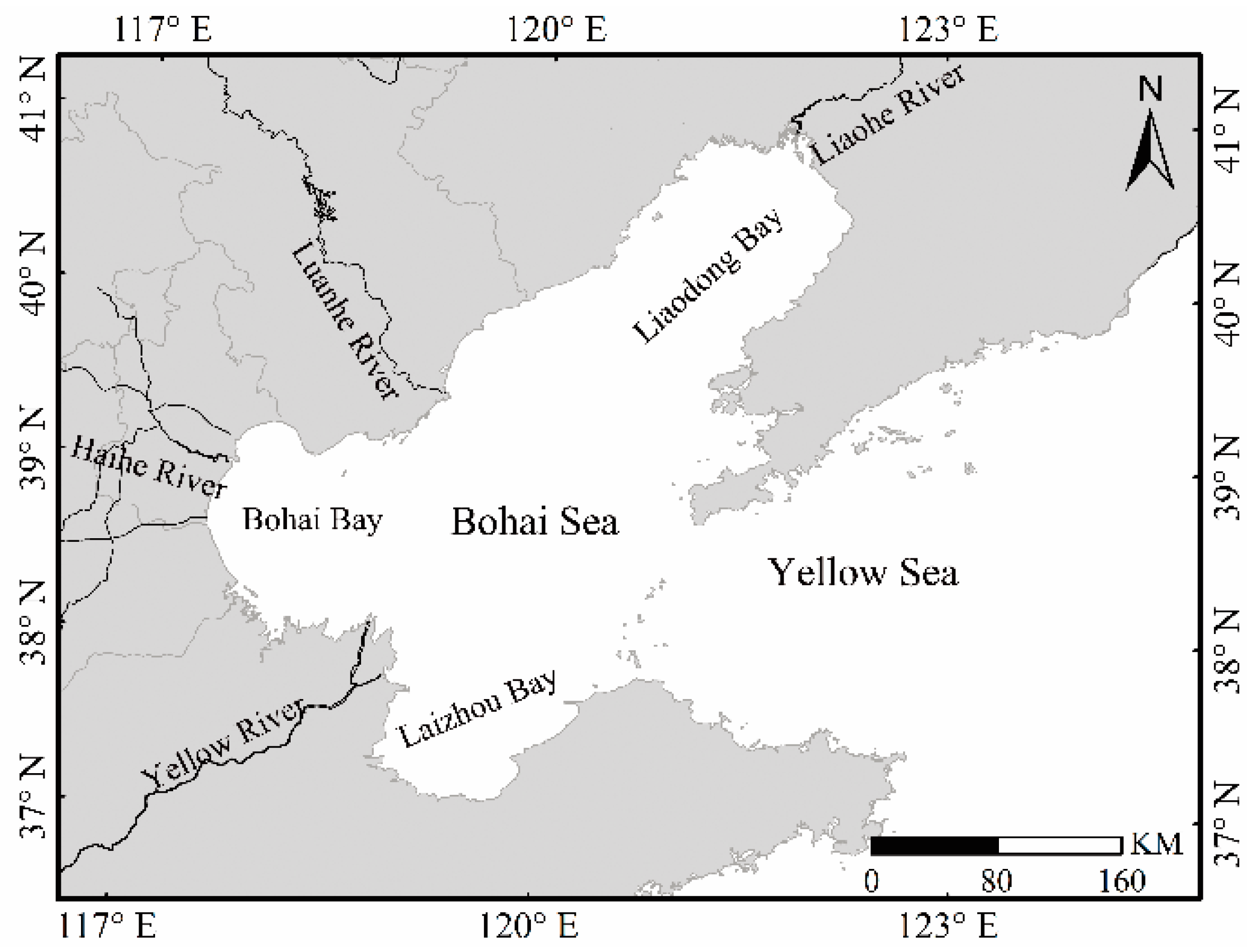
The Bohai Sea (37°07′–41°0′N, 117°35′–121°10′E), located on the northeast of China, borders three land areas and one sea (Figure 1). It covers a total area of 73,686 km2 and has an average depth of 18 m. It comprises three bays: the Liaodong Bay in the north, the Bohai Bay in the west, and the Laizhou Bay in the south. Over 40 tributaries flow into the sea, the largest four of which are the Yellow River, Haihe River, Luanhe River, and Liaohe River, which carry large quantities of freshwater and sediment into the sea from the land. The salinity of the seawater is only about 30 PSU, making it the least saline of China’s coastal waters. Seasonal sea ice usually first occurs at the coast in late December then accumulates along the shoreline and gradually expands into the central basin. Ice coverage finally comes to an end in March of the next year. The thickness of the ice can reach up to 40 cm in extremely cold winters [23], and it usually reaches its maximum extent at the midpoint of the sea ice evolutionary process in late January to early February.
The new-generation optical sensor OLCI is the successor of ENVISAT’s MERIS, having higher spectral resolution and more spectral channels. The OLCI dataset is composed of 21 distinctive spectral bands spanning the spectral range 400–1020 nm across the visible and near-infrared spectra. These multispectral data are very well suited to studying coastal sea ice. An overview of the OLCI bands is given in Table 1. Full-resolution (300 m) OLCI images (OLCI level 1b) acquired from the European Space Agency (ESA) data hub (https://scihub.copernicus.eu/) are employed for Bohai Sea ice detection in this study. Image preprocessing, including subsetting, reprojecting, and radiance-to-reflectance transformation, is conducted using the SNAP 6.0 toolbox (Sentinel Application Platform, http://step.esa.int/main/toolboxes/snap/), which was designed for processing and analyzing Sentinel satellite products.
The Sentinel-2 MultiSpectral Instrument (MSI) provides multispectral, high-resolution imagery in 13 spectral bands: four bands at 10 m, six bands at 20 m, and three bands at 60 m spatial resolution. The instrument’s imaging bands cover visible, near-infrared (NIR), and short-wave infrared (SWIR) spectra. In this study, six MSI images (MSI level 1C) acquired by Sentinel-2B over the Bohai Sea on February 1, 2018, were obtained from the ESA data hub (https://scihub.copernicus.eu/) and were processed as comparison and validation data. These images were first preprocessed by the atmospheric correction software [32] (Sen2Cor-02.05.05-win64, http://step.esa.int/main/third-party-plugins-2/sen2cor/sen2cor_v2-5-5/) and were resampled at 60 m resolution to obtain L2A products with all bands of imagery. In addition, MSI data were employed to derive the Normalized Difference Snow Index (NDSI), which was useful for sea ice detection [26,33], as a comparison.
3. Methods
3.1. Normalized Difference Sea Ice Information Index
A total of 10,570 pixels were manually selected as samples and classified as sea ice, seawater, turbid seawater, land, snow and cloud by visual interpretation. The samples were distributed across four different OLCI images in the Bohai Sea on 24 January, 28 January, 1 February, and 12 February, 2018. Descriptive statistics were computed for these samples for characteristic bands to obtain the mean and standard deviation of the top of the atmosphere (TOA) reflectance values.
The TOA reflectance of sea ice in Band 20 (930–950 nm) is higher than that in Band 21 (1000–1040 nm) in OLCI imagery; the opposite is true for all other objects, such as land and cloud cover (Figure 2a). Significant differences such as this in the spectral characteristics of land cover types are the basis for remote-sensing detection, and this particular characteristic is utilized to detect sea ice using the band ratio strategy. The Normalized Difference Sea Ice Information Index () is the normalization of this band ratio so that its value ranges between −1 and 1. The feature was extracted using the following equation:
where B20 and B21 are the TOA reflectances of Band 20 and Band 21 in OLCI images, respectively.
NDSIIIOLCI = (B20 − B21)/(B20 + B21),
The box plot in Figure 2b indicates that sea ice information is emphasized in the feature, and other cover types present in the OLCI images are de-emphasized. Sea ice has the most significant feature with the highest index value among all types of coverage. This enhancement of sea ice information and suppression of other surfaces can effectively reduce the interferences in sea ice information extraction in the Bohai Sea. Particularly, the values for sea ice are positive because its numerator is greater than zero, and the values of other cover types are negative (Figure 2b). This figure also indicates that over 75% percent of the ratio value of sea ice was greater than 0. Therefore, sea ice, which has the brightest pixels, can be directly segmented out from an feature image with a single threshold value of 0. According to the distribution of the box plot, turbid seawater is most likely to interfere with sea ice detection, as it might not be easy to separate from sea ice in .
3.2. Enhanced Normalized Difference Sea Ice Information Index
The complex water environment of the Bohai Sea makes it challenging to extract sea ice precisely using traditional remote-sensing technology. The main reason for the incomplete separation of seawater and sea ice in remote-sensing images is spectral confusion between sea ice and the suspended sediment in turbid seawater [24,27,28]. To distinguish them better, we have developed the Enhanced Normalized Difference Sea Ice Information Index () by adding consideration of Band 12 (750–757.5 nm) and Band 16 (771.25–786.25 nm) to the .
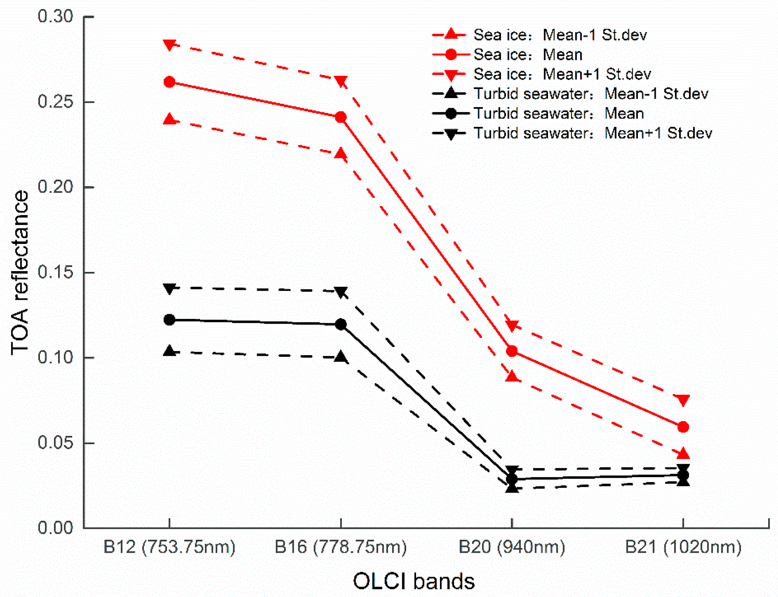
The TOA reflectance characteristics of sea ice and turbid seawater in Bands 12, 16, 20, and 21 in OLCI imagery are shown in Figure 3. It shows subtle differences in TOA reflectance between Band 12 and Band 16 and between Band 20 and Band 21 for turbid seawater but a more visible reduction in TOA reflectance between these bands for sea ice. These spectral characteristics indicate that sea ice and turbid seawater can be separated using a spectral feature that combines these band ratios. Therefore, the discriminant for identifying sea ice in turbid seawater is expressed as follows:
Linear summation was utilized to combine these two discriminants. The discrimination condition is expressed as follows:
The difference between sea ice and turbid seawater is further emphasized by summing the terms in the discrimination condition (3) to construct the Enhanced Normalized Difference Sea Ice Information Index () as follows:
where B12, B16, B20, and B21 correspond to the TOA reflectance values of Bands 12, 16, 20, and 21 in OLCI images, respectively.
B12 − B16 + B20 − B21 > 0
, which considers Band 12 and Band 16, is a further extension of . Sea ice can be distinguished from turbid seawater in by combining the two-criterion equations (2). After normalization, the index performed stably in sea ice detection from OLCI images.
3.3. Determinaton of Threshold Values
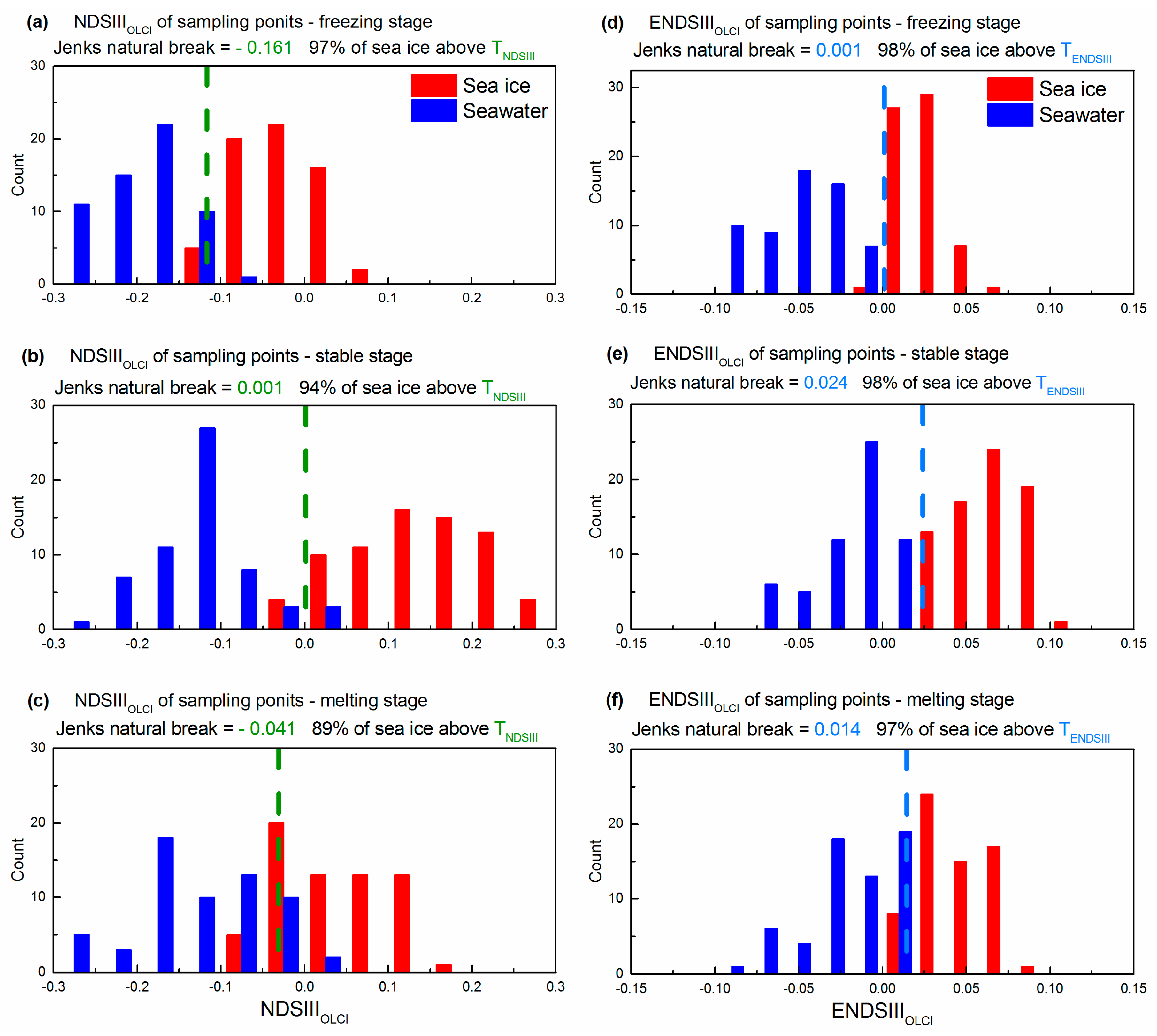
To obtain optimal threshold values for sea ice separation, the segmentation thresholds were identified through sampling of index values for and during the three main stages of the Bohai Sea ice: the freezing stage (early January), the stable stage (late January to early February), and the melting stage (late February to early March) in the winter of 2017–2018 (Figure 4). While the background coverage types, such as land, snow, and cloud, were significantly suppressed in our index and can be easily distinguished from sea ice, this was not the case for seawater, particularly turbid seawater. To address this, a total of 389 points were manually selected from nine images that included the freezing stage (1, 5 and 20 January 2018), the stable stage (28 and 31 January and 4 February 2018) and the melting stage (16 and 20 February and 21 March 2018), and classified as either sea ice or seawater by visual interpretation. Thresholds were determined from the sampling histogram using the Jenks natural break method [34], which maximizes interclass variance while minimizing intraclass variance by iteratively comparing clusters of data.
Figure 4 shows the threshold values, TNDSIII for and TENDSIII for , obtained from the sampling dataset for sea ice extraction. According to the sampling, the threshold values of and are not fixed and vary somewhat depending on the samples and ice stages. The thresholds obtained using the Jenks method performed fine in the freezing stage (Figure 4a,d), where 97% and 98% of sea ice values were above TNDSIII and TENDSIII respectively, and also acceptably performs in the stable stage (Figure 4b,e) and the melting stage (Figure 4c,f). Exceedance was still 94% and 98% of sea ice in the stable stage, and 89% and 97% of sea ice in the melting stage for the TNDSIII and TENDSIII thresholds, respectively. The sea ice can be extracted more completely using TENDSIII instead of TNDSIII.
The TNDSIII and TENDSIII were determined using the samples from the winter of 2017–2018. They were suitable for the ice detection during the 2017–2018 winter, but they may vary year by year depending on the ice conditions, such as ice developing stages, ice thickness and snow-covered situations. It is better to reset the threshold values when applying the indexes for sea ice detection in other years because the ice conditions vary with the years. The threshold values varied a little for sea ice detection in different ice stages in the 2017–2018 winter, however, the relatively stable values can provide a valuable reference for the threshold determinations of the ice extraction in other years.
3.4. Normalized Difference Snow Index
In polar and high-latitude regions, snow detection is intimately linked to sea ice detection, as the sea ice cover is mostly covered by snow. The Normalized Difference Snow Index (NDSI) has been used by many studies to detect the presence of sea ice in open water (Equation (5)) [35].
NDSI = (Green − SWIR)/(Green + SWIR)
The NDSI takes advantage of the contrasting spectral behaviors of snow and sea ice cover in the visible and short-wave infrared parts of the spectrum. Snow and sea ice will have a high NDSI value because they exhibit a large contrast in reflectance between the shot-wave infrared band (SWIR Band 11: 1.613 μm) and the visible band (Green Band 3: 0.56 μm). However, the OLCI instrument lacks the short-wave infrared bands required to derive NDSI. In this study, we used the MSI images (resampled from 60 to 300 m spatial resolution) to extract the NDSI feature, and we compared this with our efforts to detect sea ice in the Bohai Sea.
3.5. Support Vector Machine Classifier
The support vector machine (SVM) is a machine learning method based on statistical learning theory. Supervised classification using the SVM method has been widely used in image analysis to identify the class affiliated with each pixel. The basic idea of SVM classification is to use the kernel function to map linearly indivisible points in a low-dimensional space into linearly separable points in a high-dimensional space [36,37,38]. The goal of SVM classification is to find the optimal separating hyperplane that maximizes the margins between different classes. The output of SVM classification is a decision value of each pixel for each class, and it can extract good classification results from complex and noisy data.
We chose a radial basis function (RBF) to build the SVM classifier because it performs well in most cases [39]. The parameter of the Gamma (G) and penalty (C) in the kernel function were quantitatively analyzed and set to the following empirically optimized values: G = 1/feature number and C = 100 [27].
4. Results
4.1. Sea Ice Detection and Validation
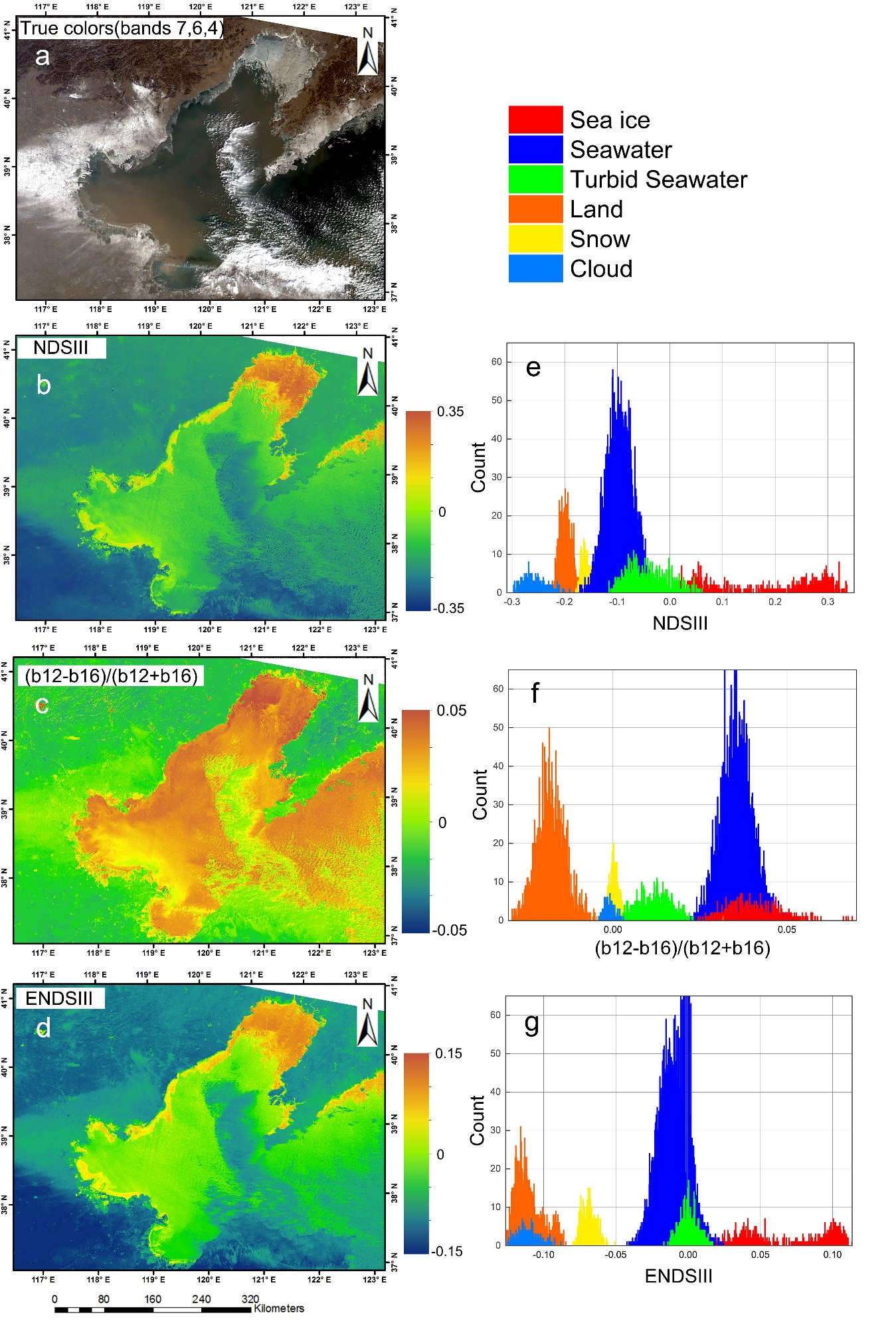
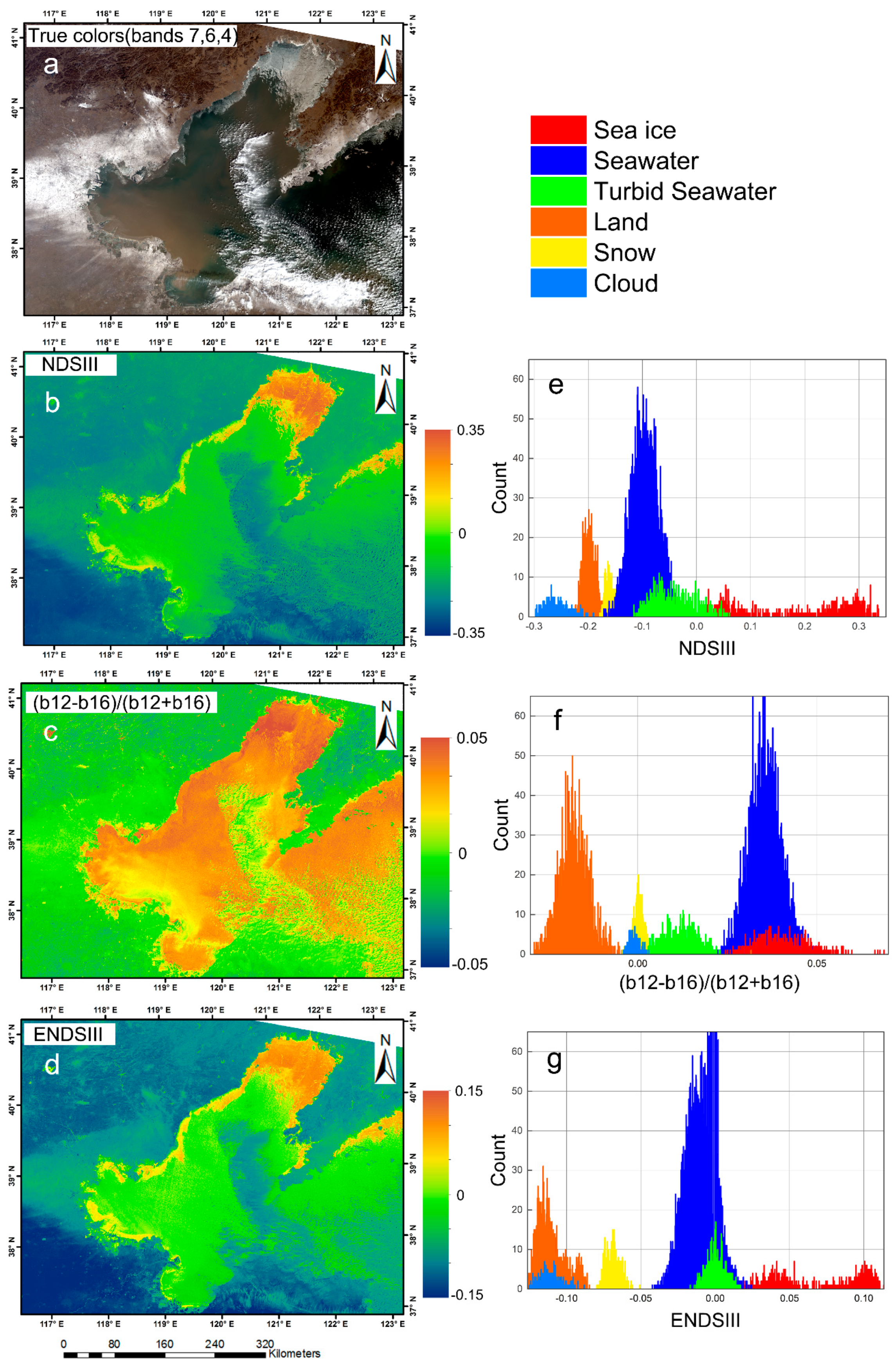
Finally, the feature images based on and were obtained from OLCI data, which significantly enhanced the sea ice information. We also added a feature image which considered the normalized ratio of Bands 12 and 16 as an important transition factor from to . Samples from the feature images were classified into the types of land cover as sea ice, seawater, turbid seawater, land, snow, and cloud through visual interpretation of OLCI true-color composite imagery. In Figure 5, sea ice is the brightest feature among the different types of land covers, suggesting its extent can be easily extracted from the feature images via threshold segmentation. The feature distribution histogram, which is a statistical representation of pixel values in feature images, was also considered for determining an appropriate threshold. In principle, sea ice information (shown in red) has the highest value of the two feature types in both normalized ratio histograms.
An additional feature of the normalized band ratio of B12 and B16 was given in response to the important role that Bands 12 and 16 play in the reduction of interference of sea ice detection in turbid seawater areas. Sea ice with bright pixels can be visually distinguished from turbid seawater with its darker pixels in the southern Bohai Sea (Figure 5c). The statistical histograms (Figure 5f) of sea ice (shown in red) and turbid seawater (shown in green) which were sampled from (B12−B16)/(B12+B16) feature image distribute separately with a boundary. This significant difference between sea ice and turbid seawater in the feature can enable us to separate them easily, but this feature could not be used to distinguish sea ice from seawater when they have approximated brightness in the feature image.
Land and cloud cover, which will be masked with great care when using other approaches, were not major sources of contamination error for sea ice identification using these OLCI imagery-based sea ice information indexes. The spectral characteristics of land and cloud enable them to be clearly identified from optical remote-sensing datasets containing rich spectral information. In the sea ice information indexes, their signals were attenuated by considering the normalized ratio of characteristic bands and were centered around −0.2 (land) and −0.3 (cloud) in and −0.125 (land and cloud) in (Figure 5b,d). The obvious visible separation between the normalized ratios of these two types of cover and that of sea ice meets the condition of sea ice extraction using optical images without masking by land or cloud.
Another cover type that will impact the accuracy of sea ice mapping with optical images is snow, which has high reflectance at visible and near-infrared wavelengths. Snow-covered ice will be confused with snow-covered land when using optical data to detect sea ice. Little snow-covered ice occurs in the Bohai Sea region in winter [40]. Furthermore, the region covered by snow on land has a low normalized ratio in the sea ice information index, generally well below the value for sea ice.
The most difficult step in sea ice extraction is to divide sea ice cover from turbid seawater. The high concentration of suspended sediment in turbid seawater leads to spectral confusion and affects sea ice identification. In the feature histogram of in Figure 5e, the normalized ratio of Band 20 to Band 21 for the area covered by sea ice is greater than 0, and those for seawater, land, snow, and cloud are less than TNDSIII which is 0.001 in the stable stage. It is noteworthy that the normalized ratio for some turbid seawater areas is also greater than TNDSIII, giving insufficient ability to distinguish sea ice from turbid seawater with a high sediment concentration. Seawater and turbid seawater may be extracted with sea ice in when a lower threshold value is used for segmentation. The misclassification caused by spectral confusion did not appear with , which also considers OLCI Bands 12 and 16. The normalized ratio for the area covered by sea ice is greater than TENDSIII which is 0.024 in the stable stage, and that of other land cover types is less than this value, including seawater and turbid seawater. Sea ice information can therefore be extracted accurately from sediment-laden water using threshold segmentation in feature images. On the basis of these results, regions with sea ice were extracted in this study by threshold segmentation of and feature images using certain thresholds.
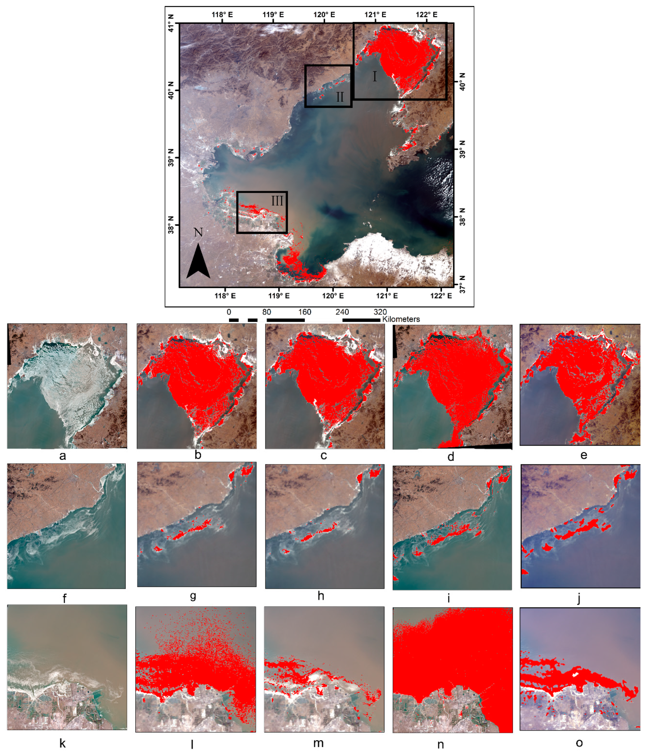
After sea ice extent extraction from OLCI imagery on the basis of threshold segmentation which was established using the Jenks natural break method from different stages of sea ice, the extraction results were compared with NDSI and SVM methods and validated using a simultaneously acquired high-resolution Sentinel-2 MSI image with a spatial resolution of 60 m after preprocessing (Figure 6).
Figure 6 shows a comparison among the different methods of sea ice extraction from satellite imagery in the Bohai Sea on February 1, 2018. Three representative scenes, including high concentration of ice (Figure 6a), low concentration of ice (Figure 6f), and sea ice in turbid water (Figure 6k), were selected from the MSI images for detection validation. The MSI image was also employed in sea ice detection via NDSI using threshold segmentation, so as to compensate for the deficiency in NDSI extraction from OLCI images (Figure 6d,i,n). Sea ice extent was also extracted from OLCI images using the SVM classification method as a comparison (Figure 6e,j,o).
Generally, the spectral-characteristic-based sea ice detection method was well capable of identifying the Bohai Sea ice in OLCI images and enabled the details of its extent, such as the ice edges and ice lanes, to be rapidly and precisely determined. The largest critical sea ice hazard, in Liaodong Bay (Figure 6a), was extracted from OLCI images using (Figure 6b), (Figure 6c), NDSI (Figure 6d), and SVM (Figure 6e), and the first three distribution maps give similar depictions of the sea ice, but omission of sea ice detection occurred when performing the SVM classifier. The three indexes had consistently good performance in critical regions with thick, extensive sea ice cover in the northern Bohai Sea. A comparison of the results shows that the sea ice area extracted by the (Figure 6l) and NDSI (Figure 6n) are larger than that extracted by the (Figure 6l) and SVM (Figure 6o). This is mainly attributed to the complex seawater environment and different sea ice features near the Yellow River estuary in Laizhou Bay (Figure 6k) where the concentration of suspended sediment reaches 100 mg l−1 in winter. The and NDSI are likely to overestimate the extent of sea ice in coastal waters where the sediment concentration is high. However, the results of the and SVM are not affected by turbid seawater contamination, and comparison with the reference images indicate that they can accurately depict the outer edge of sea ice in areas of turbid sea. In addition, omitted extraction in the extent of sea ice was observed in both indexes at the western coast of the Bohai Sea where the floe size is small or the ice cover is sparse (Figure 6f). Validation against the MSI image indicates that only thicker sea ice with higher brightness in the remote-sensing image was well identified using these approaches. Thus, thin ice was not effectually detected when extracting the Bohai Sea ice from OLCI imagery using the multispectral-bands ratio indexes employed in this study.
Comparison of the results confirms that land and cloud do not contribute to the sea ice signal. Threshold segmentation based on sea ice information indexes is efficiently capable of extracting sea ice extent without masking by land and cloud. Additionally, snow-covered land cannot influence the sea ice detection using our indexes, even though the snow was perceived to exist in the shore side region beside sea-ice-covered areas.
The validation results clearly show that the different methods achieved different sea ice detection accuracies. The accuracy of our was high, with an overall accuracy of 94.83% and a Kappa coefficient of 76.54%, close to the accuracy of SVM, and higher than or NDSI (Table 2). The results indicate that the main source of error was the mislabeling of turbid seawater as sea ice. Given the spectral confusion between sea ice and turbid seawater, the error was relatively significant in double-bands ratio methods, such as NDSI and . The SVM method reached high detection accuracy through image classification, but it needs sample training in the complex classifier, which is relatively time-consuming and inefficient. However, the has the advantage of rapid and effective detection of sea ice while outperforming the other methods. These results suggest that our method is well suited for sea ice monitoring in the Bohai Sea, even with its complex seawater environment during winter.
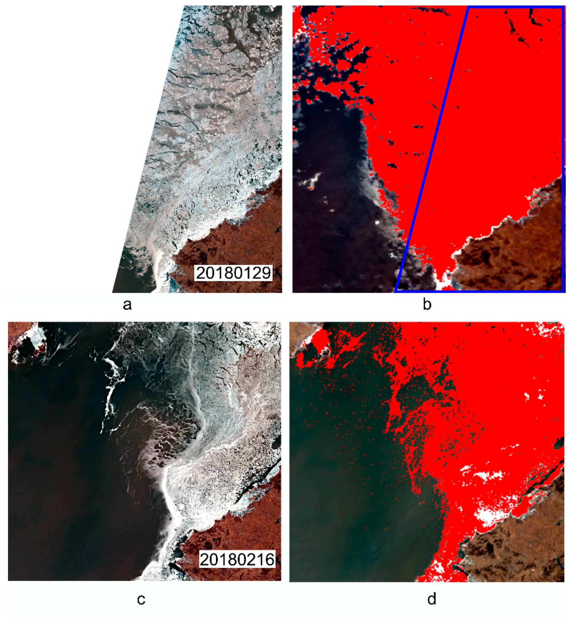
The sea ice extraction results via were also validated using another two simultaneous MSI images on different dates (29 January 2018 (Figure 7a) at ice stable stage and 16 February 2018 (Figure 7c) at ice melting stage) which are available. The sea ice extraction results from (Figure 7) show that the method can effectively extract sea ice extent at different ice stages. A few areas with high reflectance in the image were not extracted as sea ice, which may be caused by the snow cover. The snow cover area was small and had little effect on the sea ice extraction.
4.2. Spatiotemporal Evolution of the Bohai Sea Ice in the 2017–2018 Winter
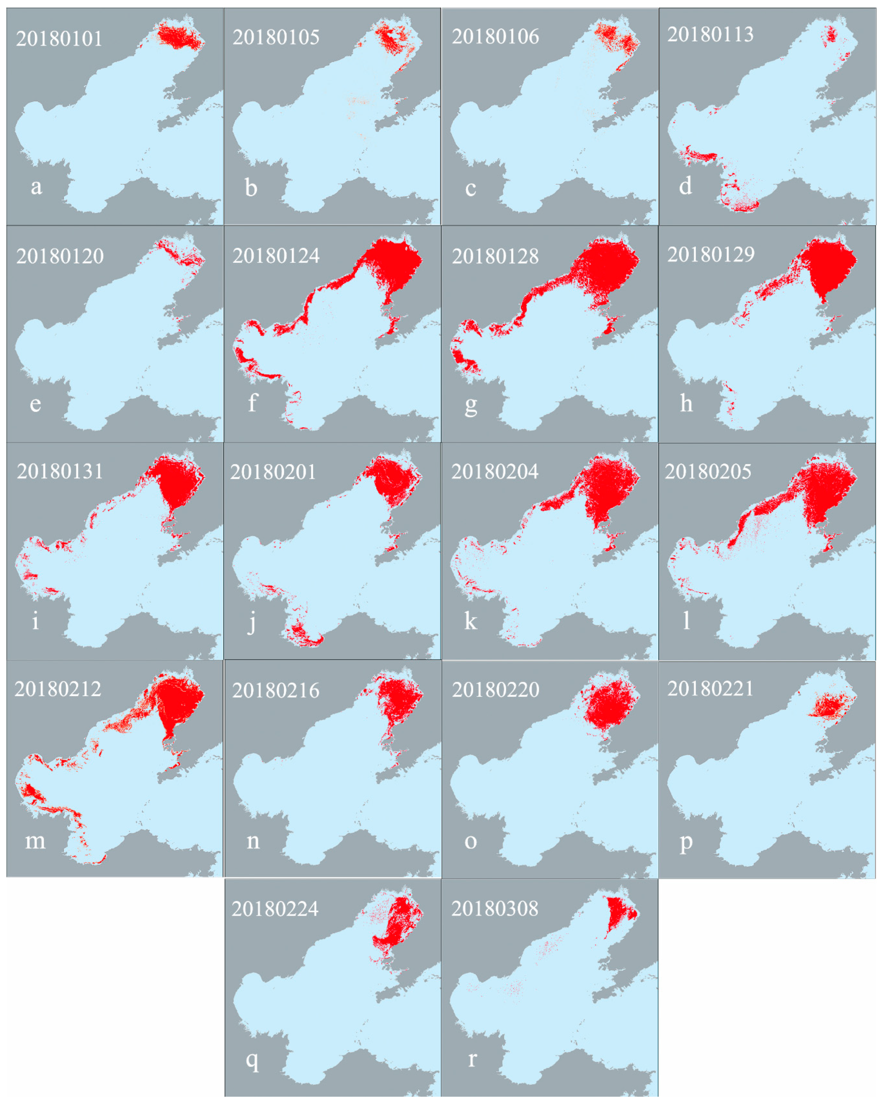
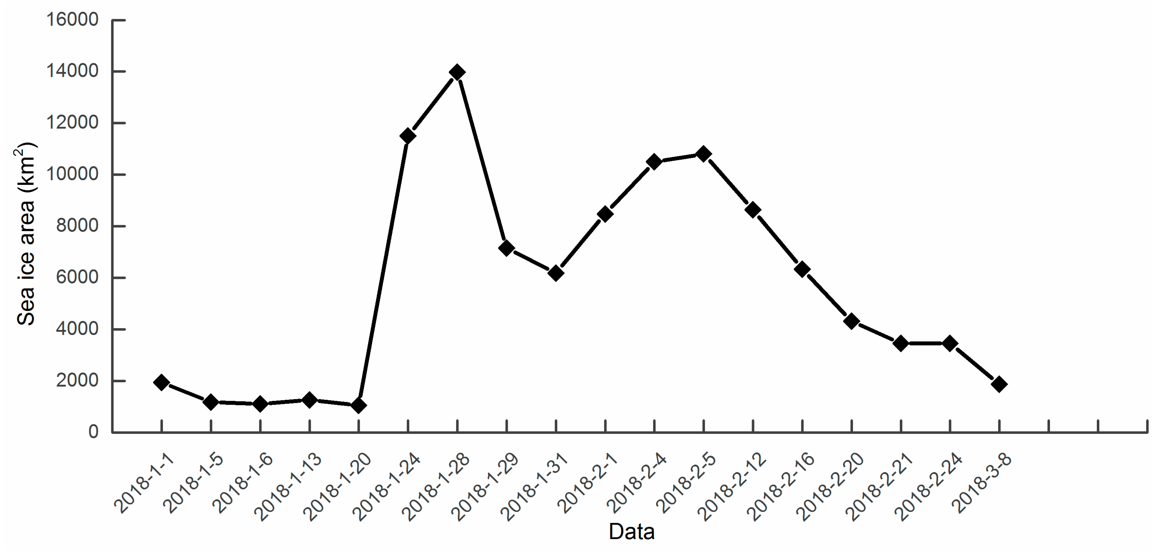
Sea ice coverage significantly expanded in the Bohai Sea from December 2017 to January 2018. The , which efficiently reduces the interference of turbid seawater in the southern Bohai Sea, was further applied to monitoring the variability in sea ice extent with 300 m spatial resolution in the Bohai Sea during the winter of 2017–2018. Owing to the limits of cloud coverage and the revisit cycle of the satellite, only 18 images were acquired by the Sentinel-3 OLCI instrument in the Bohai Sea region from 1 January 2018 to 8 March 2018. All of the images were utilized for sea ice extent extraction and determination of spatiotemporal change in sea ice coverage during the 2017–2018 winter season. Several clear-sky scenes were acquired by Sentinel-3 OLCI prior to January 1, 2018, in December 2017. At that time, only sporadic sea ice coverage could be identified near the coastal region in the Liaodong Bay (results not shown). In early January 2018, most of the sea ice was confined to the northern part of the Liaodong Bay region. The average sea ice coverage from January 1 to January 20 (Figure 8a–e) was less than 1,400 km2; because of cloud contamination over the sea ice area, there was some underestimation of the extent of sea ice on January 13 and 20.
A significant increase in sea ice coverage occurred in the Bohai Sea in mid-January 2018 (Figure 9), with a particularly pronounced expansion occurring between 20 January 2018 (Figure 8e) and 24 January 2018 (Figure 8f). In those four days, the sea ice expanded to cover a large offshore area in Liaodong Bay, as well as some areas in Bohai Bay and Laizhou Bay. On 24 January 2018, the total sea ice coverage was 10,827 km2 (Figure 8f). By 28 January 2018, it had further expanded to both northern and western Liaodong Bay, causing the total sea ice coverage in the Bohai Sea to jump to its peak value for the entire winter season, 13,060 km2 (Figure 8g). The sea ice began its first retreat in late January and early February. The sea ice coverages on January 29, January 31, and February 1 were 7,457 km2 (Figure 8h), 6,489 km2 (Figure 8i), and 5,963 km2 (Figure 8j), respectively.
The sea ice showed a notable resurgence in early February (Figure 9). Three days after the first retreat, on February 4, 2018, the sea ice had again covered half of Liaodong Bay and had reached a coverage of 10,497 km2 (Figure 8k). On 5 February 2018, the ice coverage was insistent, at 9,935 km2 (Figure 8l). After 12 February 2018, when the total coverage was 12,954 km2 (Figure 8m), into late February, the sea ice coverage rapidly reduced and became more fragmented. The sea ice melted from the south to the north, the opposite direction to its growth, with a gradual downward trend in the ice coverage from 16 February 2018 to 8 March 2018, during which period successive images showed coverages of 6,337, 4,820, 1,932, 3,063, and 1,470 km2 (Figure 8n–r, respectively). The remaining sea ice was mainly concentrated in the north of Liaodong Bay and had drifted to and accumulated in the east of Liaodong Bay under the action of external forces such as wind and waves. The sea ice had finally completely melted away in mid-March.
5. Conclusions
Two sea ice information indexes have been developed to quickly and accurately extract the extent of sea ice from OLCI remote-sensing data. Comparison of the extraction results with higher-resolution Sentinel-2 MSI imagery verifies that these indexes enable sea ice mapping with OLCI data in the Bohai Sea. The Normalized Difference Sea Ice Information Index (), which is the normalized ratio of Band 20 to Band 21 in OLCI TOA reflectance images, and the Enhanced Normalized Difference Sea Ice Information Index (), which is a modification of in which Bands 12 and 16 are also incorporated, can effectively detect sea ice information in the Bohai Sea and suppress most background information, such as coverage by land, cloud, and snow. Comparison between the results from our indexes, famous NDSI, and SVM methods indicates that sediment-laden water can interfere with sea ice extraction with the and NDSI but that the and SVM suffer from less such interference. However, these four methods have poorer performance in detecting thin sea ice in the western Bohai Sea than they do in detecting thick sea ice. The accuracy evaluation suggests that our index can rapidly and accurately detect and map the sea ice extent in the Bohai Sea during winter. The results also show our approach can extract most of the sea ice (including nilas ice, gray ice, and gray-white ice) in OLCI images, but the new ice which is small and thin is hard to interpret and detect from the medium-resolution OLCI images due to the limitation of the spatial resolution. Moreover, it would be better to reset the threshold values when employing our indexes to detect sea ice extent in other years because the ice conditions vary with the years.
The spatiotemporal evolution of the Bohai Sea ice in the winter of 2017–2018 was monitored by applying the to OLCI images. Two major increases were detected in the sea ice extent in mid-January and early February. The largest extent of the sea ice was 13,060 km2 on January 28. After reaching its peak in late January 2018, sea ice coverage remained high until early February, and the sea ice then gradually melted from south to north in mid-February. The whole period when there was ice coverage lasted for about four months, within which there was a significant expansion in mid-January and a final fading away in early March. Overall, our proposed method provides a convenient and effective technique for sea ice detection and evolution study in the Bohai Sea, which can help monitor the recent impacts of global warming.
Author Contributions
H.S. and B.J. conceived and designed the experiments; B.J. performed the experiments; H.S. and B.J. analyzed the results; H.S. and B.J. wrote the paper; H.S. and Y.W. revised the paper.
Funding
This research was funded by National Natural Science Foundation of China (41971384, 41601444, 41630963), Natural Science Foundation of Fujian Province, China (2017J01657), Outstanding Young Scientists Program in Universities of Fujian Province (KJ2017-17), and Central Guide Local Science and Technology Development Projects (2017L3012).
Acknowledgments
We thank the European Space Agency (ESA) data hub for the Sentinel-3 OLCI data and Sentinel-2 MSI imagery (https://scihub.copernicus.eu/), which are freely accessible to the public.
Conflicts of Interest
The authors declare no conflict of interest.
References
- Ning, L.; Xie, F.; Gu, W.; Xu, Y.; Huang, S.; Yuan, S.; Cui, W.; Levy, J. Using remote sensing to estimate sea ice thickness in the Bohai Sea, China based on ice type. Int. J. Remote Sens. 2009, 30, 4539–4552. [Google Scholar] [CrossRef]
- Su, H.; Wang, Y.; Yang, J. Monitoring the Spatiotemporal Evolution of Sea Ice in the Bohai Sea in the 2009–2010 Winter Combining MODIS and Meteorological Data. Estuaries Coasts 2012, 35, 281–291. [Google Scholar] [CrossRef]
- Shi, W.; Wang, M. Sea ice properties in the Bohai Sea measured by MODIS-Aqua: 1. Satellite algorithm development. J. Mar. Syst. 2012, 95, 32–40. [Google Scholar] [CrossRef]
- Ouyang, L.; Hui, F.; Zhu, L.; Cheng, X.; Cheng, B.; Shokr, M.; Zhao, J.; Ding, M.; Zeng, T. The spatiotemporal patterns of sea ice in the Bohai Sea during the winter seasons of 2000–2016. Int. J. Digit. Earth 2017, 1–17. [Google Scholar] [CrossRef]
- Liu, M.; Dai, Y.; Zhang, J.; Zhang, X.; Meng, J.; Xie, Q. PCA-based sea-ice image fusion of optical data by HIS transform and SAR data by wavelet transform. Acta Oceanol. Sin. 2015, 34, 59–67. [Google Scholar] [CrossRef]
- Teleti, P.R.; Luis, A.J. Sea ice observations in polar regions: Evolution of technologies in remote sensing. Int. J. Geosci. 2013, 4, 1031–1050. [Google Scholar] [CrossRef]
- Karvonen, J. Baltic sea ice concentration estimation based on C-band dual-polarized SAR data. IEEE Trans. Geosci. Remote Sens. 2014, 52, 5558–5566. [Google Scholar] [CrossRef]
- Ivanova, N.; Pedersen, L.; Tonboe, R.; Kern, S.; Heygster, G.; Lavergne, T.; Sørensen, A.; Saldo, R.; Dybkjær, G.; Brucker, L. Inter-comparison and evaluation of sea ice algorithms: Towards further identification of challenges and optimal approach using passive microwave observations. Cryosphere 2015, 9, 1797–1817. [Google Scholar] [CrossRef]
- Lavergne, T.; Macdonald Sørensen, A.; Kern, S.; Tonboe, R.; Notz, D.; Aaboe, S.; Bell, L.; Dybkjær, G.; Eastwood, S.; Gabarro, C.; et al. Version 2 of the EUMETSAT OSI SAF and ESA CCI sea-ice concentration climate data records. Cryosphere 2019, 13, 49–78. [Google Scholar] [CrossRef] [Green Version]
- Meier, W.N.; Fetterer, F.; Stewart, J.S.; Helfrich, S. How do sea-ice concentrations from operational data compare with passive microwave estimates? Implications for improved model evaluations and forecasting. Ann. Glaciol. 2015, 56, 332–340. [Google Scholar] [CrossRef] [Green Version]
- Agnew, T.; Howell, S. The use of operational ice charts for evaluating passive microwave ice concentration data. Atmosphere-Ocean 2003, 41, 317–331. [Google Scholar] [CrossRef]
- Berg, A.; Eriksson, L.E.B. SAR algorithm for sea ice concentration—Evaluation for the Baltic Sea. IEEE Geosci. Remote Sens. Lett. 2012, 9, 938–942. [Google Scholar] [CrossRef]
- Deng, H.; Clausi, D.A. Unsupervised segmentation of synthetic aperture radar sea ice imagery using a novel Markov random field model. IEEE Trans. Geosci. Remote Sens. 2005, 43, 528–538. [Google Scholar] [CrossRef]
- Huck, P.; Light, B.; Eicken, H.; Haller, M. Mapping sediment-laden sea ice in the Arctic using AVHRR remote-sensing data: Atmospheric correction and determination of reflectances as a function of ice type and sediment load. Remote Sens. Environ. 2007, 107, 484–495. [Google Scholar] [CrossRef]
- Shi, W.; Wang, M. Sea ice properties in the Bohai Sea measured by MODIS-Aqua: 2. Study of sea ice seasonal and interannual variability. J. Mar. Syst. 2012, 95, 41–49. [Google Scholar] [CrossRef]
- Yuan, S.; Liu, C.; Liu, X. Practical Model of Sea Ice Thickness of Bohai Sea Based on MODIS Data. Chin. Geogr. Sci. 2018, 28, 863–872. [Google Scholar] [CrossRef] [Green Version]
- Drüe, C.; Heinemann, G. High-resolution maps of the sea-ice concentration from MODIS satellite data. Geophys. Res. Lett. 2004, 31. [Google Scholar] [CrossRef]
- Zhang, D.; Ke, C.; Sun, B.; Lei, R.; Tang, X. Extraction of sea ice concentration based on spectral unmixing method. J. Appl. Remote Sens. 2011, 5, 053552. [Google Scholar] [CrossRef]
- Liu, W.; Sheng, H.; Zhang, X. Sea ice thickness estimation in the Bohai Sea using geostationary ocean color imager data. Acta Oceanol. Sin. 2016, 35, 105–112. [Google Scholar] [CrossRef]
- Lang, W.; Wu, Q.; Zhang, X.; Meng, J.; Wang, N.; Cao, Y. Sea ice drift tracking in the Bohai Sea using geostationary ocean color imagery. J. Appl. Remote Sens. 2014, 8, 083650. [Google Scholar] [CrossRef]
- Yan, Y.; Huang, K.; Shao, D.; Xu, Y.; Gu, W. Monitoring the Characteristics of the Bohai Sea Ice Using High-Resolution Geostationary Ocean Color Imager (GOCI) Data. Sustainability 2019, 11, 777. [Google Scholar] [CrossRef]
- Wang, X.; Wu, Z.; Wang, C.; Li, X.; Li, X.; Qiu, Y. Reducing the impact of thin clouds on Arctic Ocean sea ice concentration from FengYun-3 MERSI data single cavity. IEEE Access 2017, 5, 16341–16348. [Google Scholar] [CrossRef]
- Su, H.; Wang, Y. Using MODIS data to estimate sea ice thickness in the Bohai Sea (China) in the 2009–2010 winter. J. Geophys. Res. Oceans 2012, 117. [Google Scholar] [CrossRef]
- Su, H.; Wang, Y.; Xiao, J.; Li, L. Improving MODIS sea ice detectability using gray level co-occurrence matrix texture analysis method: A case study in the Bohai Sea. ISPRS J. Photogramm. Remote Sens. 2013, 85, 13–20. [Google Scholar] [CrossRef]
- Han, Y.; Li, J.; Zhang, Y.; Hong, Z.; Wang, J. Sea ice detection based on an improved similarity measurement method using hyperspectral data. Sensors 2017, 17, 1124. [Google Scholar] [CrossRef]
- Gignac, C.; Bernier, M.; Chokmani, K.; Poulin, J. IceMap250—Automatic 250 m sea ice extent mapping using MODIS data. Remote Sens. 2017, 9, 70. [Google Scholar] [CrossRef]
- Su, H.; Wang, Y.; Xiao, J.; Yan, X. Classification of MODIS images combining surface temperature and texture features using the Support Vector Machine method for estimation of the extent of sea ice in the frozen Bohai Bay, China. Int. J. Remote Sens. 2015, 36, 2734–2750. [Google Scholar] [CrossRef]
- Zhang, N.; Wu, Y.; Zhang, Q. Detection of sea ice in sediment laden water using MODIS in the Bohai Sea: A CART decision tree method. Int. J. Remote Sens. 2015, 36, 1661–1674. [Google Scholar] [CrossRef]
- Toming, K.; Kutser, T.; Uiboupin, R.; Arikas, A.; Vahter, K.; Paavel, B. Mapping water quality parameters with sentinel-3 ocean and land colour instrument imagery in the Baltic Sea. Remote Sens. 2017, 9, 1070. [Google Scholar] [CrossRef]
- Bi, S.; Li, Y.; Wang, Q.; Lyu, H.; Liu, G.; Zheng, Z.; Du, C.; Mu, M.; Xu, J.; Lei, S.; et al. Inland Water Atmospheric Correction Based on Turbidity Classification Using OLCI and SLSTR Synergistic Observations. Remote Sens. 2018, 10, 1002. [Google Scholar] [CrossRef]
- Lin, J.; Lyu, H.; Miao, S.; Pan, Y.; Wu, Z.; Li, Y.; Wang, Q. A two-step approach to mapping particulate organic carbon (POC) in inland water using OLCI images. Ecol. Indic. 2018, 90, 502–512. [Google Scholar] [CrossRef]
- Vuolo, F.; Zóltak, M.; Pipitone, C.; Zappa, L.; Wenng, H.; Immitzer, M.; Weiss, M.; Baret, F.; Atzberger, C. Data service platform for Sentinel-2 surface reflectance and value-added products: System use and examples. Remote Sens. 2016, 8, 938. [Google Scholar] [CrossRef]
- Riggs, G.A.; Hall, D.K.; Ackerman, S.A. Sea ice extent and classification mapping with the moderate resolution imaging spectroradiometer airborne simulator. Remote Sens. Environ. 1999, 68, 152–163. [Google Scholar] [CrossRef]
- Jenks, G.F. The data model concept in statistical mapping. Int. Yearb. Cartogr. 1967, 7, 186–190. [Google Scholar]
- Dozier, J. Spectral signature of alpine snow cover from the landsat thematic mapper. Remote Sens. Environ. 1989, 28, 9–22. [Google Scholar] [CrossRef]
- Burges, C.J.C. A tutorial on support vector machines for pattern recognition. Data Min. Knowl. Discov. 1998, 2, 121–167. [Google Scholar] [CrossRef]
- Vapnik, V.N. An overview of statistical learning theory. IEEE Trans. Neural Netw. 1999, 10, 988–999. [Google Scholar] [CrossRef]
- Weston, J.; Watkins, C. Support vector machines for multi-class pattern recognition. In Proceedings of the 7th European Symposium on Artificial Neural Networks (ESANN-99), Bruges, Belgium, 21–24 April 1999; Volume 99, pp. 219–224. [Google Scholar]
- Zhang, H.; Zhang, Y.; Lin, H. Compare different levels of fusion between optical and SAR data for impervious surfaces estimation. In Proceedings of the 2nd International Workshop on Earth Observation and Remote Sensing Applications, EORSA 2012, Shanghai, China, 8–11 June 2012; pp. 26–30. [Google Scholar] [CrossRef]
- Yuan, S.; Gu, W.; Liu, C.; Xie, F. Towards a semi-empirical model of the sea ice thickness based on hyperspectral remote sensing in the Bohai Sea. Acta Oceanol. Sin. 2017, 36, 80–89. [Google Scholar] [CrossRef]
Figure 1.
The study area of the Bohai Sea, including the Liaodong Bay, Bohai Bay, and Laizhou Bay.

Figure 2.
TOA reflectance values in OLCI all bands (a) and values (b) for sea ice, seawater, turbid seawater, land, snow, and cloud cover in the Bohai Sea. The whiskers in (a) depict the standard deviations of the TOA reflectance samples. The whiskers in (b) indicate the maximum and minimum ratio values of the sample. The box is determined by the 25th and 75th percentiles of the ratio values of the sample. The median value is marked as the line within the box.

Figure 3.
Sample TOA reflectance values for sea ice and turbid seawater in OLCI Bands 12, 16, 20, and 21 in the Bohai Sea.
Figure 3.
Sample TOA reflectance values for sea ice and turbid seawater in OLCI Bands 12, 16, 20, and 21 in the Bohai Sea.

Figure 4.
The histogram distributions of sampling points for the three sea ice development stages (freezing, stable and melting stages) with (a–c) and (d–f). The TNDSIII and TENDSIII threshold values (dashed vertical lines) were determined for sea ice separation by the Jenks natural break method.
Figure 4.
The histogram distributions of sampling points for the three sea ice development stages (freezing, stable and melting stages) with (a–c) and (d–f). The TNDSIII and TENDSIII threshold values (dashed vertical lines) were determined for sea ice separation by the Jenks natural break method.

Figure 5.
An example of true-color (a), (b), (b12−b16)/(b12+b16) (c), and (d) feature extraction from OLCI imagery on 24 January 2018. A statistical histogram of the main types of surface cover (sea ice, seawater, turbid seawater, land, snow, and cloud) in each image is displayed alongside the corresponding image (e–g).

Figure 6.
An image of sea ice extraction result for the entire Bohai Sea (top) on 1 February 2018 using threshold segmentation from . Three true-color images in the first column (a,f,k) are the enlarged MSI validation images indicated by boxes I, II, and III in the top image, respectively. The next four columns present the results of sea ice extent extraction using (b,g,l), (c,h,m), NDSI (d,i,n), and SVM (e,j,o).

Figure 7.
Sea ice extraction results based on from OLCI images with 300 m spatial resolution on 29 January 2018 (b) and February 16, 2018 (d). Two true-color images in the first column (a,c) are the MSI validation images with 60 m spatial resolution. The blue box in (b) represents the boundary of the validation image (a).

Figure 8.
Spatiotemporal evolution of the extent of Bohai Sea ice during the winter of 2017–2018 from OLCI images using the method (a–r). Red areas depict sea ice coverage.
Figure 8.
Spatiotemporal evolution of the extent of Bohai Sea ice during the winter of 2017–2018 from OLCI images using the method (a–r). Red areas depict sea ice coverage.

Figure 9.
The evolution of the Bohai Sea ice area extracted from OLCI images during the winter of 2017–2018.
Figure 9.
The evolution of the Bohai Sea ice area extracted from OLCI images during the winter of 2017–2018.


Table 1.
OLCI band characteristics.
| Band Number | Central Wavelength (nm) | Full Width at Half Maximum (nm) | Signal-to-Noise Ratio |
|---|---|---|---|
| Band 1 | 400 | 15 | 2188 |
| Band 2 | 412.5 | 10 | 2061 |
| Band 3 | 442.5 | 10 | 1811 |
| Band 4 | 490 | 10 | 1541 |
| Band 5 | 510 | 10 | 1488 |
| Band 6 | 560 | 10 | 1280 |
| Band 7 | 620 | 10 | 997 |
| Band 8 | 665 | 10 | 883 |
| Band 9 | 673.75 | 7.5 | 707 |
| Band 10 | 681.25 | 7.5 | 745 |
| Band 11 | 708.75 | 10 | 785 |
| Band 12 | 753.75 | 7.5 | 605 |
| Band 13 | 761.25 | 2.5 | 232 |
| Band 14 | 764.375 | 3.75 | 305 |
| Band 15 | 767.5 | 2.5 | 330 |
| Band 16 | 778.75 | 15 | 812 |
| Band 17 | 865 | 20 | 666 |
| Band 18 | 885 | 10 | 395 |
| Band 19 | 900 | 10 | 308 |
| Band 20 | 940 | 20 | 203 |
| Band 21 | 1020 | 40 | 152 |
Table 2.
Contingency table for accuracy validation of sea ice detection based on different methods on 1 February 2018.
Table 2.
Contingency table for accuracy validation of sea ice detection based on different methods on 1 February 2018.
| Ground Truth | ||||||
|---|---|---|---|---|---|---|
| Sea Ice | Other | Total | Commission Error | |||
| Map | Sea Ice | 89 | 11 | 100 | 11.00% | |
| Other | 35 | 754 | 789 | 4.44% | ||
| Total | 124 | 765 | 889 | |||
| Omission Error | 28.23% | 1.44% | Overall Accuracy | |||
| Kappa | 76.54% | 94.83% | ||||
| Map | Sea Ice | 94 | 35 | 129 | 27.13% | |
| Other | 30 | 730 | 760 | 3.95% | ||
| Total | 124 | 765 | 889 | |||
| Omission Error | 24.19% | 4.58% | Overall Accuracy | |||
| Kappa | 70.05% | 92.69% | ||||
| NDSI | Map | Sea Ice | 107 | 77 | 184 | 41.85% |
| Other | 18 | 798 | 816 | 2.21% | ||
| Total | 125 | 875 | 1000 | |||
| Omission Error | 14.40% | 8.80% | Overall Accuracy | |||
| Kappa | 63.88% | 90.50% | ||||
| SVM | Map | Sea Ice | 97 | 19 | 116 | 16.38% |
| Other | 28 | 762 | 790 | 3.54% | ||
| Total | 125 | 781 | 906 | |||
| Omission Error | 22.40% | 2.43% | Overall Accuracy | |||
| Kappa | 77.51% | 94.81% | ||||
© 2019 by the authors. Licensee MDPI, Basel, Switzerland. This article is an open access article distributed under the terms and conditions of the Creative Commons Attribution (CC BY) license (http://creativecommons.org/licenses/by/4.0/).
Share and Cite
MDPI and ACS Style
Su, H.; Ji, B.; Wang, Y. Sea Ice Extent Detection in the Bohai Sea Using Sentinel-3 OLCI Data. Remote Sens. 2019, 11, 2436. https://0-doi-org.brum.beds.ac.uk/10.3390/rs11202436
AMA Style
Su H, Ji B, Wang Y. Sea Ice Extent Detection in the Bohai Sea Using Sentinel-3 OLCI Data. Remote Sensing. 2019; 11(20):2436. https://0-doi-org.brum.beds.ac.uk/10.3390/rs11202436
Chicago/Turabian StyleSu, Hua, Bowen Ji, and Yunpeng Wang. 2019. "Sea Ice Extent Detection in the Bohai Sea Using Sentinel-3 OLCI Data" Remote Sensing 11, no. 20: 2436. https://0-doi-org.brum.beds.ac.uk/10.3390/rs11202436
Note that from the first issue of 2016, this journal uses article numbers instead of page numbers. See further details here.