A New Processing Chain for Real-Time Ground-Based SAR (RT-GBSAR) Deformation Monitoring


1
School of Engineering, Newcastle University, Newcastle upon Tyne NE1 7RU, UK
2
Ocean Geomatics Center, The First Institute of Oceanography, State Oceanic Administration in China, Qingdao 266061, China
3
School of Land Science and Technology, China Univ. of Geosciences, Xueyuan Rd. 29, Beijing 100083, China
4
Hunan Key Laboratory of Coal Resources Clean-utilization and Mine Environment Protection, Hunan University of Science and Technology, Xiangtan Hunan, 411201, China
*
Author to whom correspondence should be addressed.
Remote Sens. 2019, 11(20), 2437; https://0-doi-org.brum.beds.ac.uk/10.3390/rs11202437
Submission received: 12 September 2019
/
Revised: 15 October 2019
/
Accepted: 16 October 2019
/
Published: 20 October 2019
(This article belongs to the Special Issue Advances in Real Aperture and Synthetic Aperture Ground-Based Interferometry)
Abstract
:Due to the high temporal resolution (e.g., 10 s) required, and large data volumes (e.g., 360 images per hour) that result, there remain significant issues in processing continuous ground-based synthetic aperture radar (GBSAR) data. This includes the delay in creating displacement maps, the cost of computational memory, and the loss of temporal evolution in the simultaneous processing of all data together. In this paper, a new processing chain for real-time GBSAR (RT-GBSAR) is proposed on the basis of the interferometric SAR small baseline subset concept, whereby GBSAR images are processed unit by unit. The outstanding issues have been resolved by the proposed RT-GBSAR chain with three notable features: (i) low requirement of computational memory; (ii) insights into the temporal evolution of surface movements through temporarily-coherent pixels; and (iii) real-time capability of processing a theoretically infinite number of images. The feasibility of the proposed RT-GBSAR chain is demonstrated through its application to both a fast-changing sand dune and a coastal cliff with submillimeter precision.
1. Introduction
In comparison to spaceborne synthetic aperture radar (SAR), ground-based SAR (GBSAR) has an inherent flexibility of allowing adjustable temporal resolution in data acquisition. Depending on the rate of change in any particular case study, or the practical environment for instrument deployment, GBSAR data acquisition can be performed in either continuous or discontinuous mode [1,2,3,4]. According to Crosetto, et al. [1], the continuous mode of operation is the more commonly deployed technique. The continuous mode employs a zero-baseline geometry for all acquisitions, thus avoiding influences of hardware related technical issues and leading to better performance in terms of the density, precision, and reliability of deformation measurements [5,6]. This study therefore focuses only on continuous GBSAR deformation monitoring.
In the continuous mode, consecutive acquisitions with a high temporal resolution (up to several seconds) enable time series analysis of fast-changing scenarios that can provide insight into mechanisms and triggering factors of hazardous events, or even act as the basis for early warning systems. However, in practice, the processing of continuous GBSAR data has the following characteristics:
(1) A large number of image acquisitions are usually performed in a continuous campaign due to the requirement or desire for high temporal resolution GBSAR data. For instance, the current FastGBSAR system [7] can repeat an acquisition at the finest resolution every ten seconds, implying that up to 360 images can be acquired every hour. There are two significant challenges in processing such a large volume of consecutive GBSAR images: (a) the management of computational random-access memory (RAM) for such a large number of images, and (b) the inevitable presence of targets that are temporarily coherent for a certain length of time, but not for the entire observation period.
(2) Real-time processing of GBSAR imagery may be required in urgent situations, e.g., landslide early-warning systems, where the creation of displacement maps is required in as short a time frame as possible.
(3) Continuous data collection is performed by fixing the radar instrument in a stationary position. In this case, the spatial baseline is always zero and the topographic effect is absent in the interferometric phase [2,3]. Therefore, spatial baseline operations such as the co-registration of master and slave images, the removal of topographic phase contribution, and the estimation of orbital errors in spaceborne Interferometric SAR (InSAR) processing can be omitted in a continuous GBSAR interferometric processing chain.
(4) Atmospheric phase screen (APS) is usually considered spatially correlated and temporally uncorrelated for spaceborne SAR [8,9]. The estimation of APS in spaceborne SAR data is often performed through temporal high pass and spatial low pass filtering, which is not applicable in the GBSAR case due to the extremely short time intervals between SAR acquisitions [10].
Regarding data processing in continuous GBSAR, representative approaches are summarized. (i) Simultaneous processing of all data together in a typical InSAR time series procedure (e.g., [11,12]), which, however, leads to three issues: delay in production of displacement maps, extreme cost of computational memory, and the loss of temporal evolution. (ii) Temporal averaging of images [13], which can improve the signal-to-noise ratio (SNR) and reduce the volume of continuous GBSAR data at the expense of temporal resolution. This is not appropriate in fast-changing scenarios where large deformation occurring in a short period can lead to coherence losses and unreliable measurements. (iii) A real-time approach developed by Roedelsperger, et al. [14], which involves a two-step phase unwrapping strategy. In the approach, ordinary persistent scatterers (PSs) are distinguished from a subset of selected persistent scatterer candidates (PSCs). Unwrapping results are obtained by only selected PSCs and then expanded to all other ordinary PSs. Thus, the solutions for PSs are smoothed and dependent on the reliability of PSC results, which is a drawback of this approach. Additionally, sudden phase changes can occur on any single PSC pixel and probably cause regional unwrapping errors and propagate to the final cumulative deformation.
With consideration of these characteristics and unaddressed issues, a new processing chain has been developed for real-time continuous GBSAR deformation monitoring, termed real-time GBSAR (RT-GBSAR). This paper describes the main endeavors addressing RAM management, real-time capability, and the reliability of processing consecutive GBSAR data with high temporal resolution and large data volumes.
2. Materials and Methods
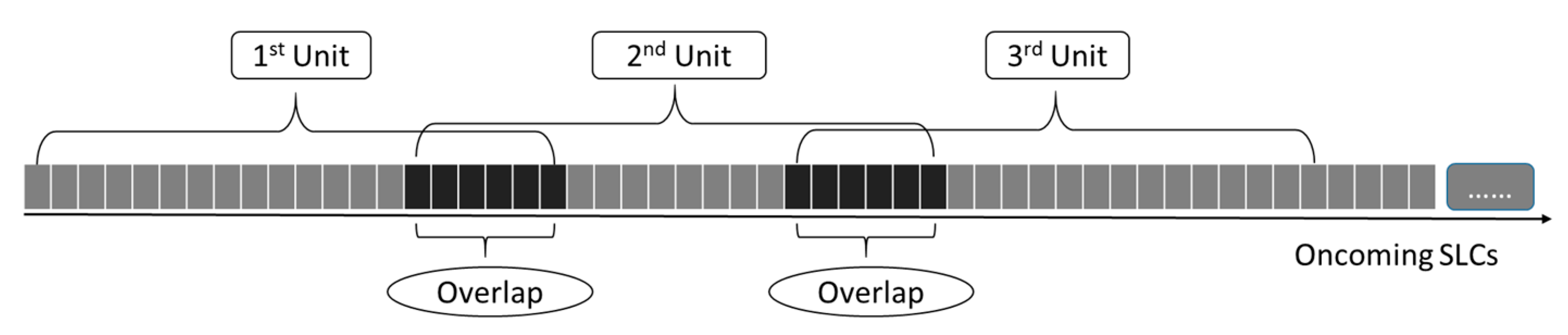
The proposed RT-GBSAR chain exploits the small baseline subset (SBAS) concept and processes consecutive GBSAR single-look complex (SLC) images on a unit by unit basis. SLC images within a temporal window form a basic unit in the chain. The flow is controlled by two parameters: the window size and the temporal baseline constraint. The window size represents the number of SLC images in a unit, and the temporal baseline constraint specifies the number of preceding images that are allowed to form interferograms with the current image. The overlap of two neighboring units is fixed as a twofold temporal baseline constraint. A schematic of the proposed strategy is illustrated in Figure 1. A complete time series analysis is performed within each unit and adjacent units are connected via the overlapping SLC images.
By adopting this strategy, the RT-GBSAR chain has several merits. Firstly, the RAM requirement is limited to only one unit of SLC images, and the chain can theoretically process an infinite number of oncoming images. Secondly, it affords the opportunity to investigate the evolution of surface movements since it preserves temporarily-coherent pixels, which are present in one or more units, but not in the entire observation period. Thirdly, this chain supports real-time processing of the oncoming data, and any latency in the creation of displacement maps can be minimized since there is no requirement to wait for the entire dataset before processing commences.
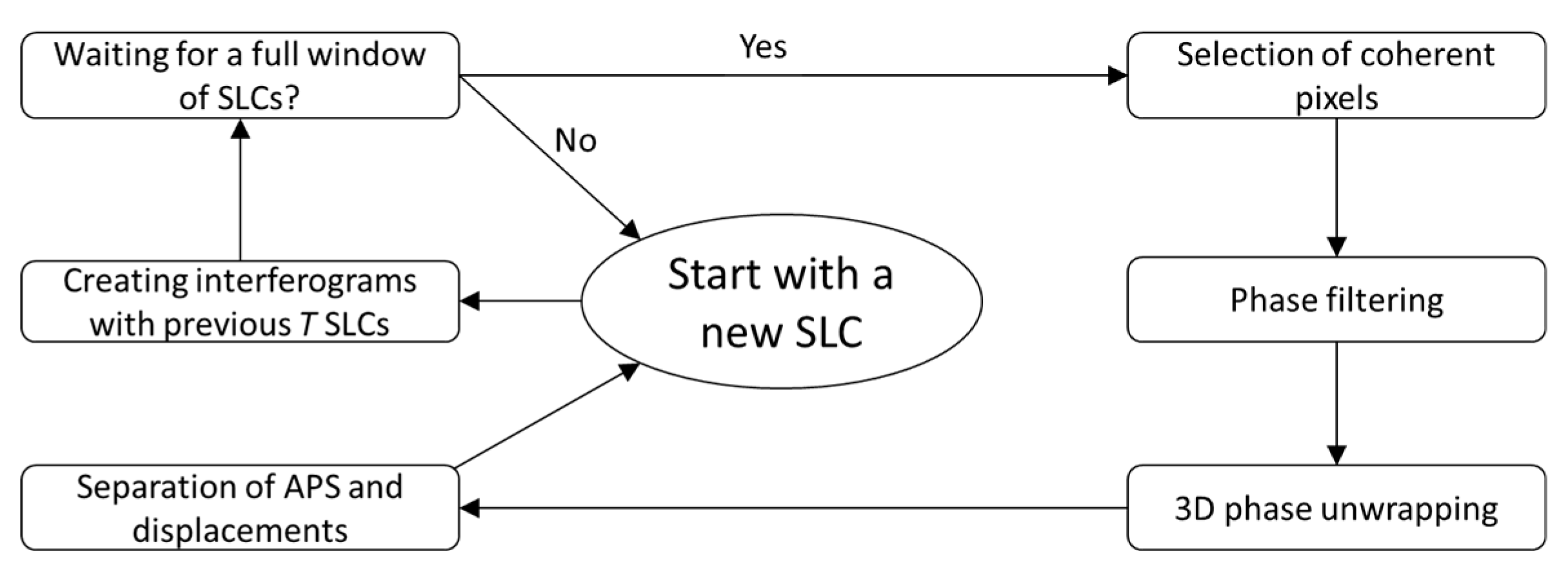
The SBAS concept in the proposed RT-GBSAR chain is illustrated in Figure 2. The procedure in each unit starts with a new SLC image. Once a new SLC image is received, interferograms can be generated using the new SLC and its previous SLC images (where denotes the temporal baseline constraint). In practice, the selection of the temporal baseline is made on the basis of both computational efficiency and the required accuracy [15]. A longer temporal baseline constraint results in a more redundant network of interferograms at the expense of computational efficiency. Additionally, the temporal baseline should be relatively short for rapidly changing scenarios as temporal decorrelations can be significant. In the process, the SBAS procedure will not begin until the number of available SLC images is sufficient (i.e., equivalent to a full time window).
To achieve reliable time series results, advanced InSAR algorithms are integrated into the proposed SBAS procedure. Specifically, a temporal baseline constraint is set to construct a redundant network of interferograms. The accurate coherence of each interferogram is calculated by the non-local “MIAS” method [16]. A set of coherent pixels are detected for further analysis via the full-rank criterion proposed in Wang, et al. [15]. The interferometric phase of the detected coherent pixels is firstly de-noised using the non-local “MIAS” filter [16] and then unwrapped using the “StaMPS” 3D unwrapping approach [17]. Thereafter, a least-squares solution for each pixel can be achieved in the time series estimation using only the coherent phase of this pixel [15]. Note that the solution at this stage is the superposition of APS and displacements. To obtain precise displacements, atmospheric artefacts should be compensated appropriately [18]. In this SBAS procedure, the APS for scenarios with flat topography is corrected by modelling it as a linear function of the radar-to-target range under the medium homogeneity hypothesis [19]. Otherwise, APS in cases with significant topographic variations can be considered using a range- and height-dependent model and compensated with the support of ground height information [20]. In practice, a subset of highly-coherent pixels is selected from stable areas to recover the APS models by means of linear regression. The stable areas can be identified through a priori knowledge and visual inspection of the superposition of APS and displacements [15,21].
The time series estimation produces a least-squares solution [15], which is the optimal solution within the individual unit. However, the solution for an individual unit is not necessarily globally optimal when deformation information spanning multiple consecutive units is required. To address this issue, adjacent units can be linked by their common coherent pixels in the proposed RT-GBSAR chain. The adjacent units are then merged into a longer unit and the optimal solution for the resultant merged unit can be achieved. For example, assume two units are defined with a window size of 30 and a temporal baseline constraint of 3 (i.e., overlap size of 6). The first unit runs from the 1st to the 30th image and the second unit from the 25th to the 54th image. These two units can be merged into a new contiguous unit running from the 1st to the 54th image. As time series analysis is performed within each unit independently, the selected coherent pixels in these two units (denoted as and , respectively) may be different. To pursue an optimal solution for the newly merged contiguous unit, the time series analysis may be performed again on the basis of the intersection of the two coherent pixel sets, i.e., .
3. Results
A FastGBSAR system [7] was used for data collection in this study. The radar system operates at Ku band and allows an adjustable temporal and spatial resolution in data acquisition. In the case of the finest spatial resolution (i.e., 0.5 m in range and 4.8 rad in azimuth), the upper limit of temporal resolution is 10 seconds. Experiments on two short-term but large-volume continuous FastGBSAR datasets were conducted to demonstrate the feasibility of the proposed RT-GBSAR chain for continuous deformation monitoring. The case studies include a sand dune and a coastal cliff.
The algorithms used in the experiments were introduced in Section 2. The key parameters for SBAS analysis comprised a typical set of MIAS parameters (similarity threshold: 0.85; non-local window size: 15 × 15 pixels; and a minimum of 10 siblings for a reliable coherence estimation and phase filtering), and a coherence threshold of 0.45 for the selection of temporarily-coherent pixels. Considering the moderate observing size and height variation of the two case studies, height-related APS was ignored. APS was thus corrected by regressing a linear range-dependent model (namely , where , are coefficients and is the slant range between the radar and the target) with 10% of the selected temporally-coherent pixels.
3.1. Sand Dune Case Study
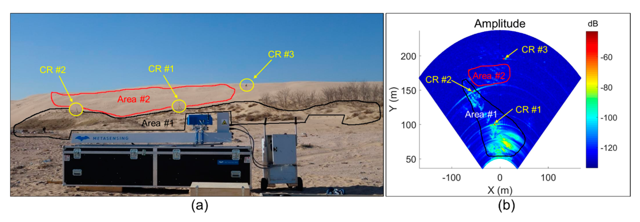
The first dataset was collected on 5 January 2015 and consisted of a sand dune area at Feicuidao on the Changli Gold Coast, Hebei Province, China. It was reported that this area experienced a fast-changing process during the period of 2006–2008 with a significant movement of up to 10.68 meters at the leeward slope bottom and up to 7.12 meters at the crest of the dune [22]. Movements were related to the regional wind regime, the morphological characteristics of the dune, and human activities. An overview of this site can be seen in Figure 3. The image size of the dataset was 371 × 306 pixels and the spatial resolution 0.5 m in the range direction and 5 mrad in the azimuth direction. The dataset consisted of 478 continuous SLC images with a temporal resolution of 10 seconds over an observation period of 1 hour 38 minutes. Somehow, a few images were occasionally not recorded by the system, probably due to the hardware insufficiency in data acquisition at such a high temporal and spatial resolution. The dataset was processed using the proposed RT-GBSAR chain with a temporal baseline constraint of five, implying that any one image can be allowed to generate interferograms with its five previous and five subsequent images. Overlap size was fixed as a twofold temporal baseline constraint, namely 10 images, in this experiment. The entire dataset of 478 images was processed in 10 units with a unit size of 60 images. Information about these units is summarized in Table 1.
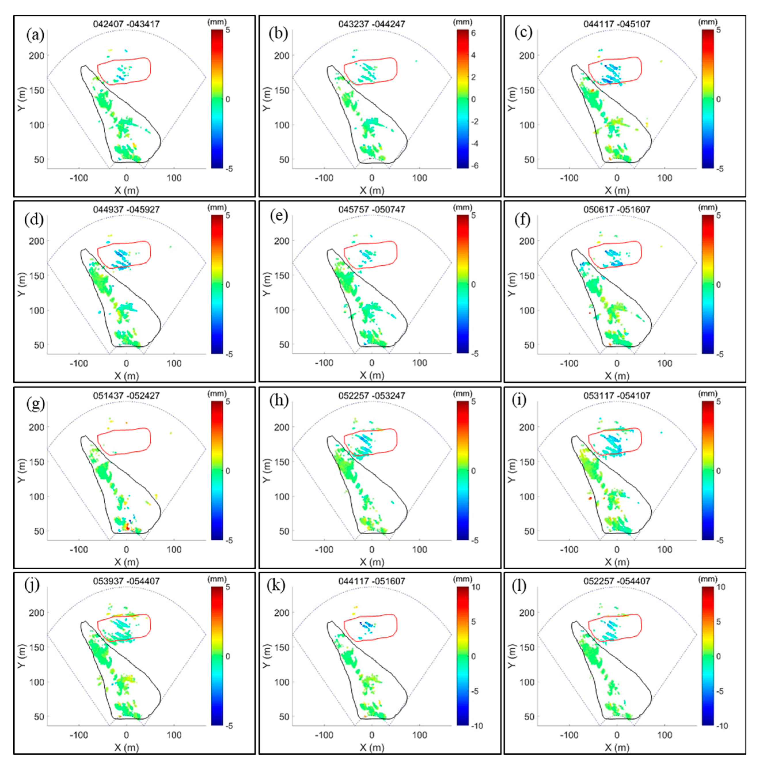
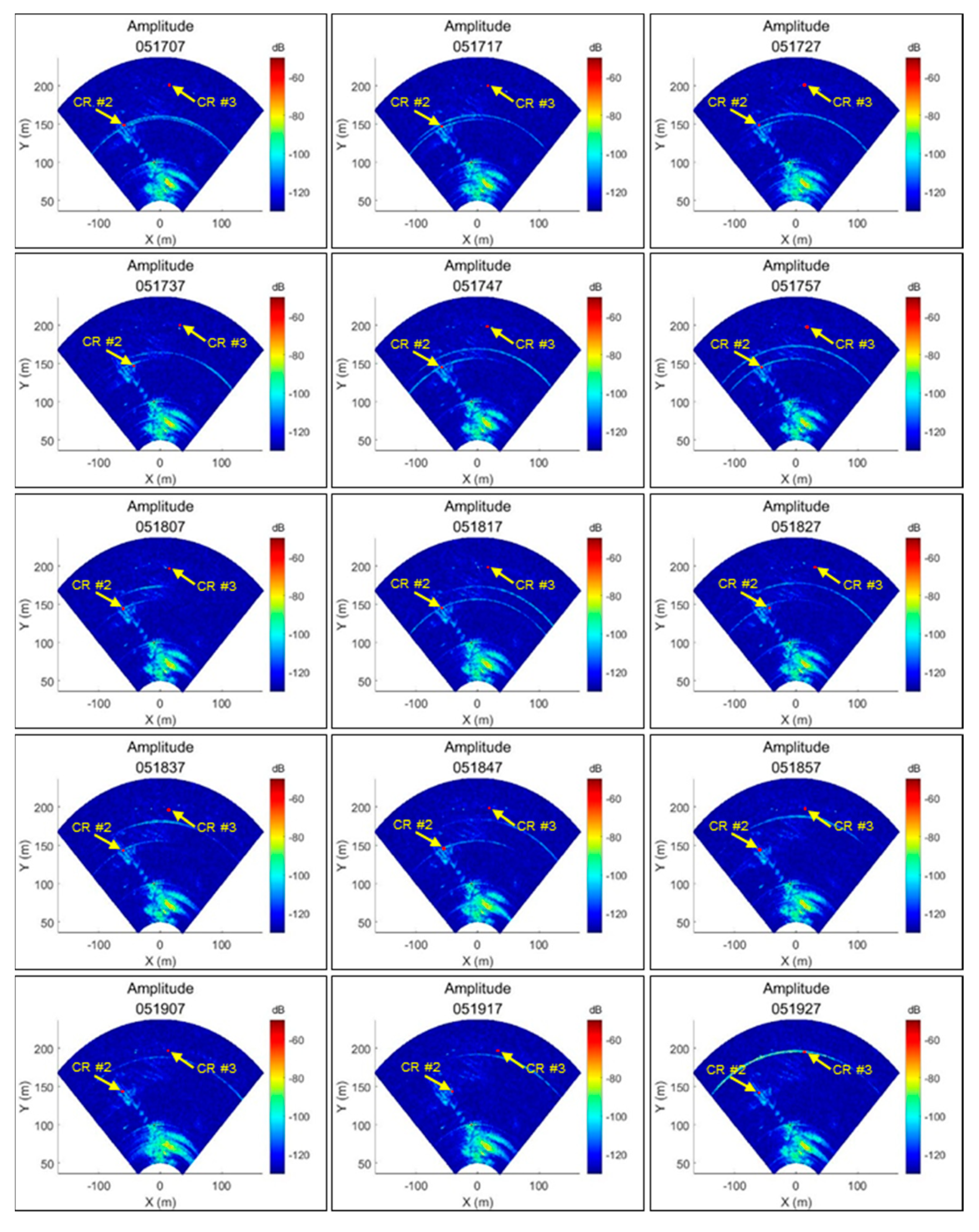
Displacement maps for all 10 units of the dune dataset are shown in Figure 4. It should be noted that coherent pixels in Area #2 disappeared in unit 7. This was because the corner reflector CR #2 was moved to the location of CR #3 during the period of data collection in unit 7. The process is illustrated by the sequential amplitude images shown in Figure 5. The moving corner reflector produced side-lobe patterns and contaminated Area #2. Therefore, very few coherent pixels were present in Area #2 of unit 7. Thus, two cumulative displacement maps (before and after unit 7) are also plotted in Figure 4. The displacement map of units 3–6 is shown in Figure 4k and that for units 8–10 in Figure 4l. It is apparent that Area #1 was generally stable over the entire observation period, with deformation primarily exhibited in Area #2. Here, a maximum cumulative displacement of up to 8 mm within a period of 35 minutes spanning units 3–6 can be seen in Figure 4k and 5 mm over another period of 22 minutes spanning units 8–10 in Figure 4l. Negative displacement values imply that targets moved closer to the radar system along the line-of-sight direction. Thus, the observed deformation most likely arose due to the process of sand sliding down the slope, which is consistent with the direction of the prevalent wind observed during fieldwork.
Area #1 was covered with sparse and shallow vegetation while Area #2 comprised only loose sand devoid of any vegetation. During the short period of data collection, the Beaufort wind force scale was recorded at the level of light air, approximately 1–2 miles per hour. In addition, both areas were occasionally intruded by humans over the observation period. Therefore, the sand motion can be attributed to three factors, namely natural slope instability of the dune, wind force, and human intrusion/activity. No matter what triggered the sand motion, the FastGBSAR results provide evidence that the presence of vegetation in coastal dunes plays an important role in helping stabilize the surface against sand motion.
3.2. Coastal Cliff Case Study
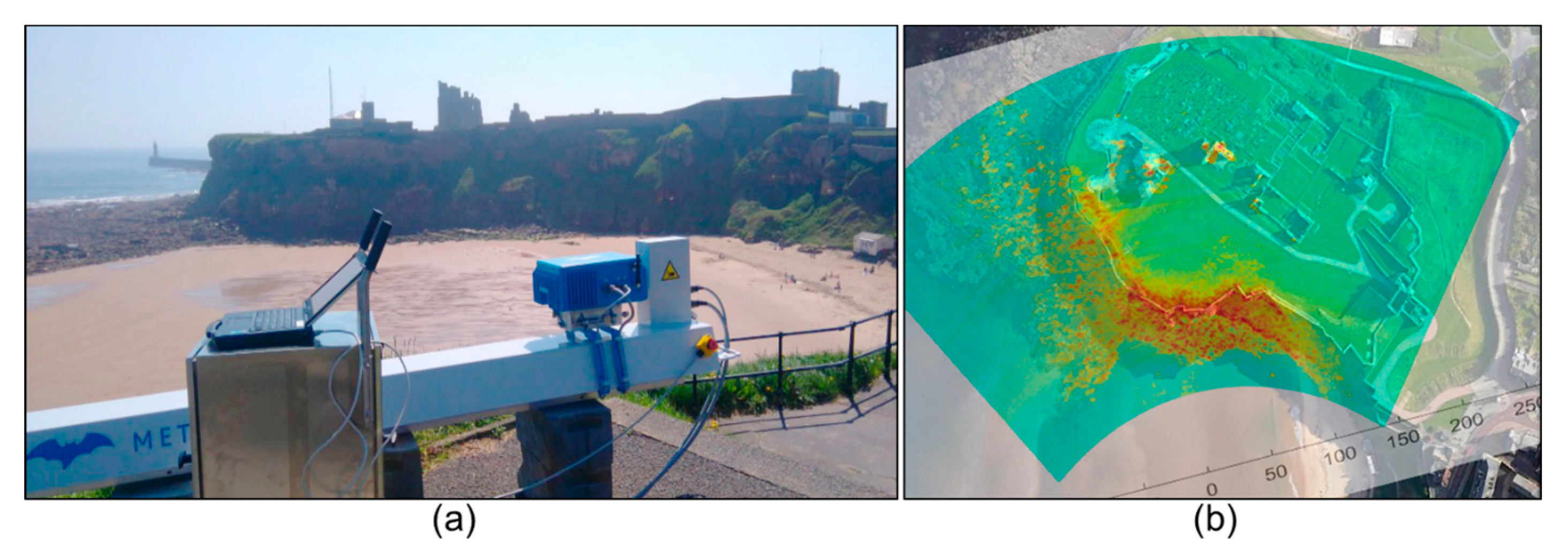
The second dataset was collected on 16 November 2016 by continuously observing the cliff on the north side of Tynemouth Priory and Castle, Tynemouth, UK. The FastGBSAR observation lasted two hours from 12:31:24 to 14:29:24 with a temporal resolution of 10 seconds and a spatial resolution of 0.75 m in range and 5 mrad in azimuth. A few acquisitions were not recorded by the system due to hardware related issues. The resultant dataset consisted of 696 continuous SLC images. An overview of the data collection is illustrated in Figure 6. It should be noted that GBSAR monitoring of this study site was previously reported in two papers [15,16]. However, the two studies processed the data over the entire observation period together and failed to extract the temporal evolution of the surface processes. This paper, on the other hand, presents the new and noteworthy findings from the RT-GBSAR processing of the large-volume data.
The dataset was processed using RT-GBSAR adopting the same parameters as the dune dataset, i.e., a unit size of 60 images and a temporal baseline constraint of five images. The entire dataset of 696 images was processed in 14 units. The information about each unit is given in Table 2.
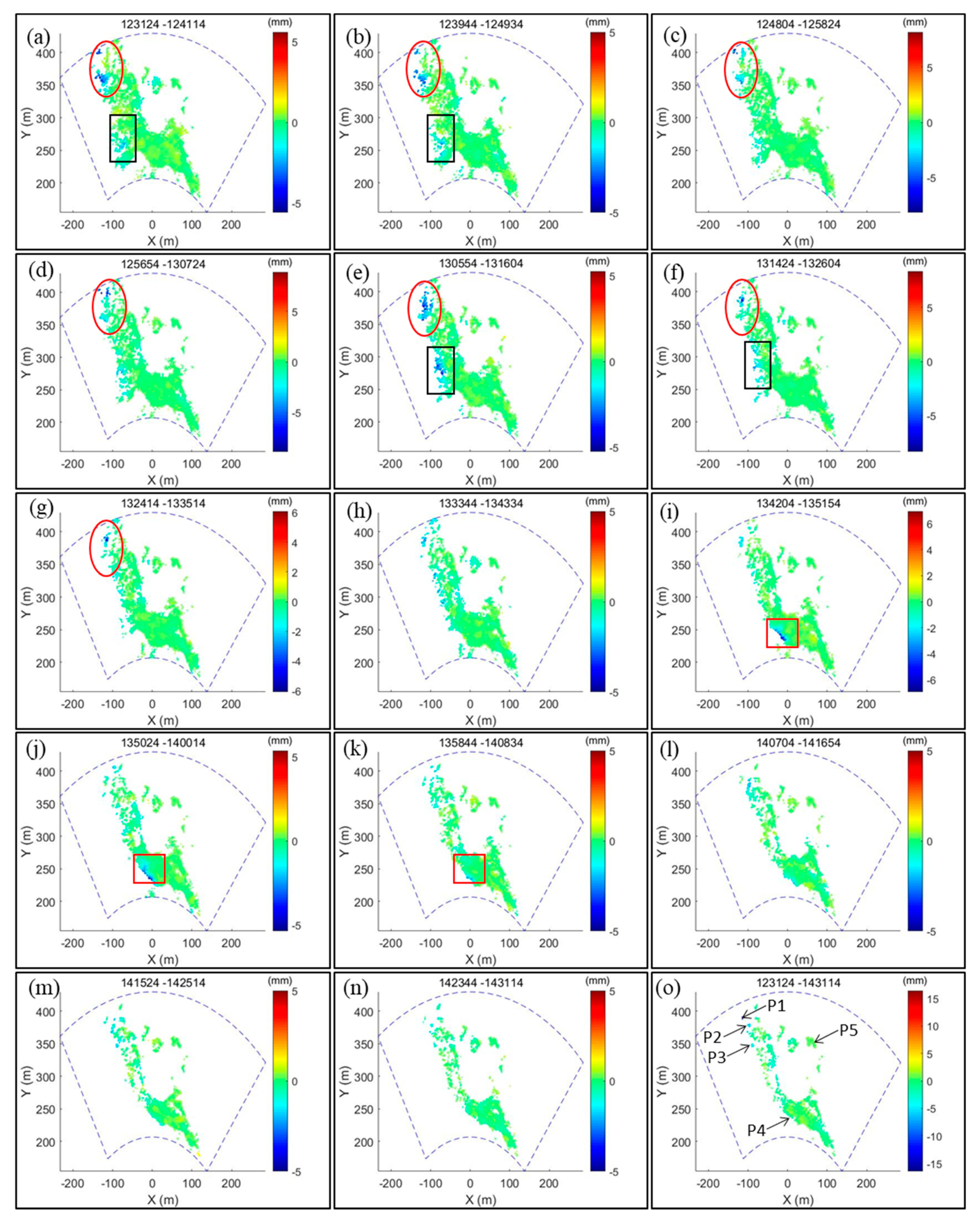
To display the temporal evolution, the displacement maps for all 14 units of the cliff dataset are shown in Figure 7. In addition, the final cumulative displacement map for pixels that are coherent over the entire observation period is also given in Figure 7o.
As shown in Figure 7, three areas of interest (AOIs) with deformation signals were visible in some units but not in the final cumulative displacement map. Specifically, the deformation signals indicated by the red ellipse were obvious from the 1st to the 7th unit and faded from the 8th unit onwards. The deformation signals indicated by the black rectangle were weak at the beginning and became active in the 5th unit, and the deformation signals indicated by the red square temporarily existed from the 9th to the 10th unit. The practical locations of these AOIs were near the sea. Among them, the AOI indicated by the red ellipse was the lowest and nearest to the sea, and the red square was the highest and furthest from the sea. During the observation period, the water level rose with the sea tides and gradually submerged these areas. The tidal elevation for the observation area on the day of data collection is given in Figure 8.
With the increasing water level, the number of coherent pixels in each unit generally decreased. The number of coherent pixels shared by all units totaled only 3428. However, only a very few pixels with significant deformation could be found in the total cumulative displacement map in Figure 7o, and the temporal evolution of the marked AOIs near the sea were nearly lost. This demonstrates the importance of exploiting temporarily-coherent pixels and processing continuous GBSAR data on a unit by unit basis. Otherwise, the temporal evolution of ground deformation cannot be detected.
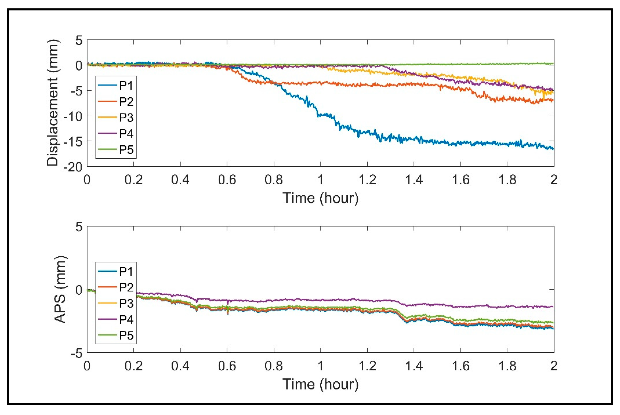
In order to investigate the time series process, a set of pixels (P1, P2, P3, P4, and P5) were selected from the results of units 1–14 in Figure 7o. Pixels P1–P4 corresponded to ground targets that were near the sea, while P5 was located on a building. The time series of displacements and APS for these pixels are shown in Figure 9. According to the displacement time series, pixels P1–P4 were stable for the first 0.6 h. After that these pixels gradually moved as the sea tide approached to these targets. In contrast, pixel P5 remained stable for the entire observation period. Besides, the APS time series showed that the smallest APS was experienced by P4 as it was the nearest target to the radar system, while the greatest was experienced by P1 as it was the furthest among the selected targets. This is consistent with the APS correction model (, where , are coefficients and is the slant range between the radar and the target) used in this experiment.
The deformation maps, time-series displacements, and relevant analysis therefore suggest that the ground deformation is related to the sea tides. Without proper validation data, it is difficult to interpret the deformation signals. The findings, which may be useful for the interpretation, are summarized as follows: (i) the physical feature of the moving targets was rock; (ii) targets moved always from the sea and towards the coast during the observation period with incoming tide; (iii) the occurrence of movement was consistent with the sequence of the sea tide approaching these targets; and (iv) deformations behaved as local signals.
4. Discussion
In this section, the performance of the developed RT-GBSAR chain is discussed, the analysis focusing on the identification of unwrapping errors in experiments and the assessment of precision in InSAR time series. The real-time capability of the proposed chain is also discussed with different parameter configurations.
4.1. Identification of Unwrapping Errors
Computation of a successful InSAR time series analysis heavily relies on the performance of phase unwrapping. In this study, the detection and identification of unwrapping errors was accomplished. Assuming a set of three interferograms formed by three complex SAR images , the raw phase for a pixel on the three complex images is denoted as and the interferometric phase on the three interferograms is (). If phase unwrapping is correct for all three interferograms, the relationship should be held by any coherent pixel on these interferograms [24,25]. The three interferograms form a closed temporal loop. Unwrapping errors always result in multiples of 2π phase misclosures and can be identified by summing round a closed temporal loop or checking a misclosure map [24]. Note that spatial filtering is often applied before phase unwrapping, which breaks the phase triangularity in a closed loop [26,27]. Therefore, the phase misclosure threshold for the identification of unwrapping errors is empirically and conservatively set as , namely an unwrapping error was defined by in this study.
For a unit of 60 images with a temporal baseline constraint of five images, there are 560 closed temporal loops. This study sums the unwrapping errors along all the temporal loops, which can be used to identify any unwrapping errors that are present. Note that the displacement maps shown in Figure 4 and Figure 7 are only for coherent pixels without unwrapping errors. The number of coherent pixels, both with and without unwrapping errors, for units in the two case studies are shown in Table 3 and Table 4, respectively. As can be seen from the results in Table 3 and Table 4, phase unwrapping is correct for the vast majority of selected coherent pixels in the dune monitoring application. The average percentage of correct unwrapping is 99.47% for the dune dataset and 99.95% for the cliff dataset. The results achieved by the RT-GBSAR chain for the two datasets can thus be considered reliable. Between the two results, a few more unwrapping errors can be identified in the sand dune dataset, an issue related to data quality. The scene of the coastal cliff dataset primarily consisted of rocks, concrete structures, and buildings, which can provide backscattering radar signals with better SNR than the sand dune with its smooth sand or sparse vegetation. Moreover, human intrusion onto the sand dune also added noise to this dataset.
4.2. Precision of Time Series Analysis
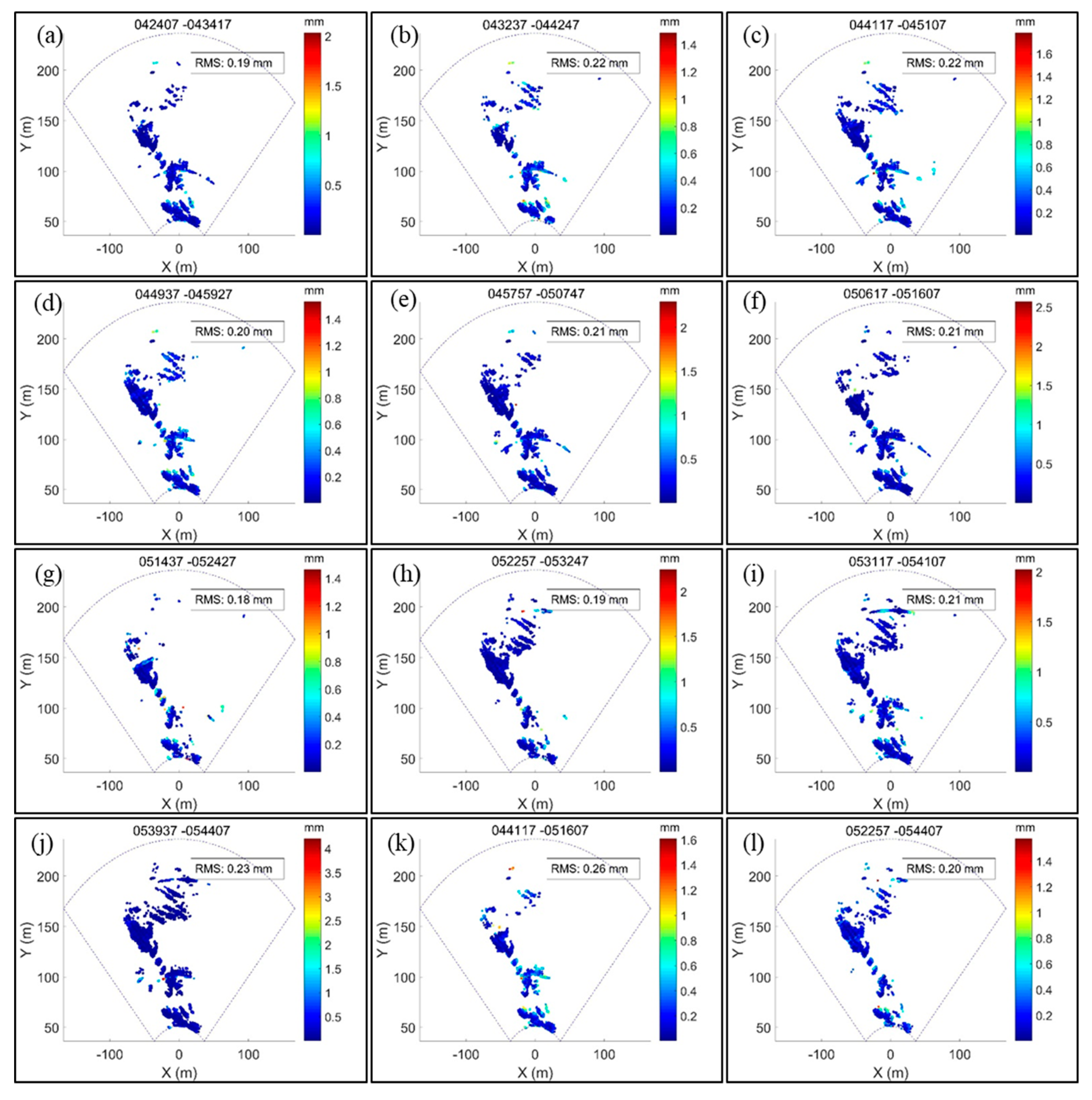
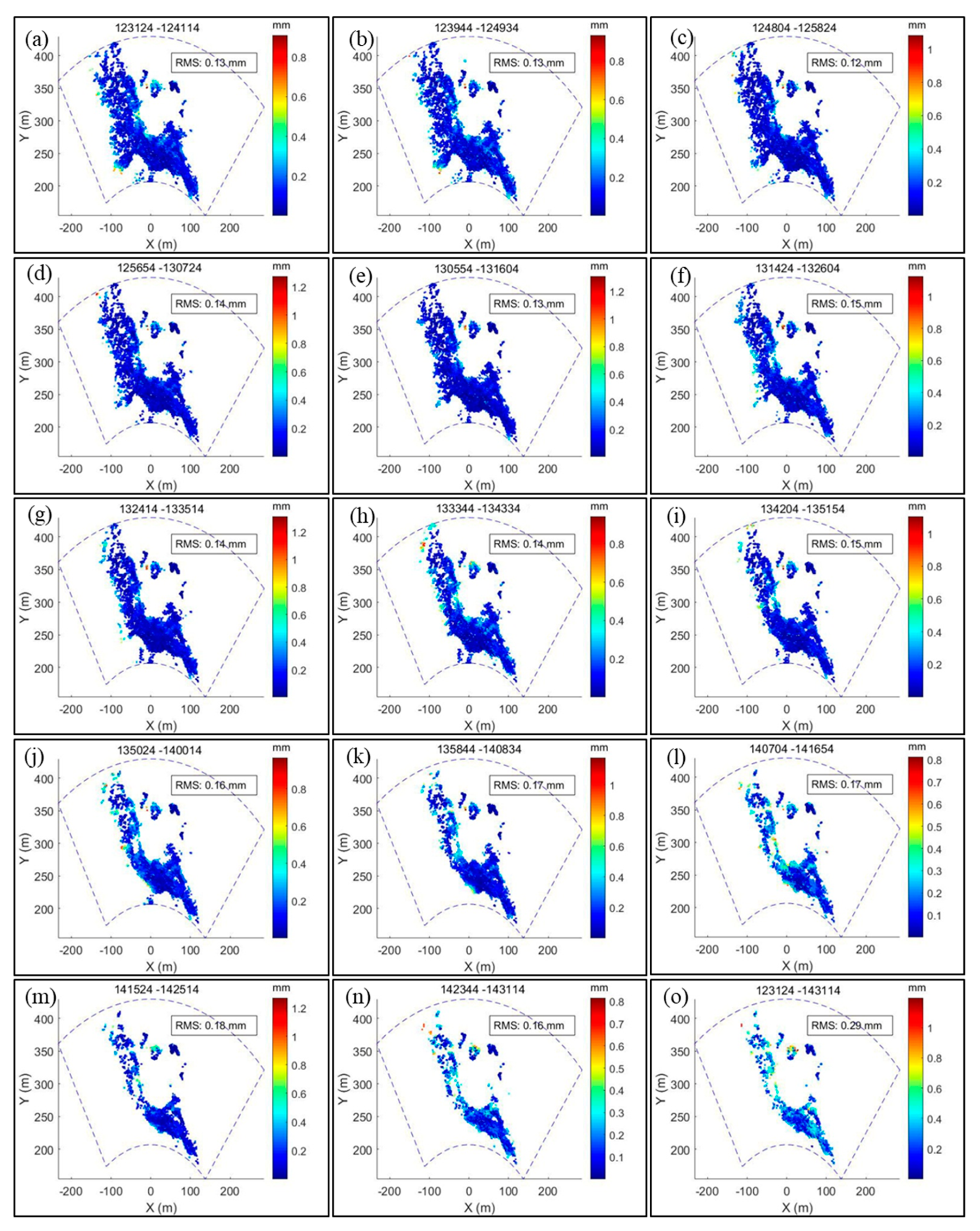
The inversion precision of SBAS time series analysis for a pixel is defined in Wang, et al. [15]. The precision maps for both applications are shown in Figure 10 and Figure 11, respectively. The overall precision indicator for all the coherent pixels is the root mean square (RMS) of the inversion precision values, which is deduced on the basis of misclosure of the redundant interferometric phase in the time series estimation. A small precision value represents good consistency in the redundant observations. According to the precision maps shown in Figure 10 and Figure 11, the overall precision reaches a few submillimeters, which supports the feasibility of the proposed chain for high-precision GBSAR deformation monitoring.
4.3. Real-Time Capability of RT-GBSAR
The proposed RT-GBSAR chain supports the real-time processing of a continuous stream of GBSAR images. Real-time capability depends on the time series strategy and its implementation. The latency (time cost) is thus twofold: (i) the acquisition time for a full window of images (denoted as ); and (ii) the processing time for time series analysis (denoted as ). Accordingly, the real-time capability is actually controlled by two parameters in the proposed chain, namely the window size of a unit (denoted as ) and the temporal baseline constraint (denoted as ). Note that the overlap size is fixed as the twofold temporal baseline constraint (i.e., 2). The acquisition time for a full window of images in a unit is thus , where denotes the temporal resolution. The effects of the two parameters on the real-time capability, the density of coherent pixels, and the overall precision for the coherent pixels in the time series estimation were analyzed using 100 images of the sand dune dataset. The temporal resolution was 10 s, i.e., . The results for multiple sets of the two parameters are summarized in Table 5.
The following conclusions can be reached, according to the results presented in Table 5: (1) The total time cost comprises the data acquisition time () and the data processing time (). It is intuitive that a higher temporal resolution leads to a shorter latency since data is provided more quickly to begin processing. The latency is also dependent on the difference between the unit size and the overlap size . The processing time increases with the number of interferograms (“Total ifgs”), which mainly depends on the temporal baseline constraint. Therefore, the real-time capability can be jointly enhanced by improving the temporal resolution and reducing the temporal baseline constraint. (2) The density of coherent pixels (i.e., “CPs” over all units) increases with the temporal baseline constraint when using the full-rank approach [15]. A longer temporal baseline constraint will lead to increased redundancy in the interferogram network and to more reliable results (indicated by a lower RMS value), but at the expense of the computational efficiency (indicated by a longer processing time ). An insufficiently small unit size (e.g., = 5) may reduce the density of coherent pixels over all units. Thus, a small unit size is only recommended if the monitoring campaign involves an extremely fast-changing site with a high real-time demand, e.g., for early warning purposes. Otherwise, the unit size can be increased.
It is worth noting that processing time depends on the adopted programming language, the algorithm implementation, and the computer configuration. Here, the proposed approach was implemented using C++ programming language and graphics processing unit (GPU) acceleration. Processing time cost was recorded by running the program on a laptop with an Intel i7 2.40 GHz CPU and an NVIDIA GeoForce 940M graphic card.
4.4. Computational RAM of RT-GBSAR
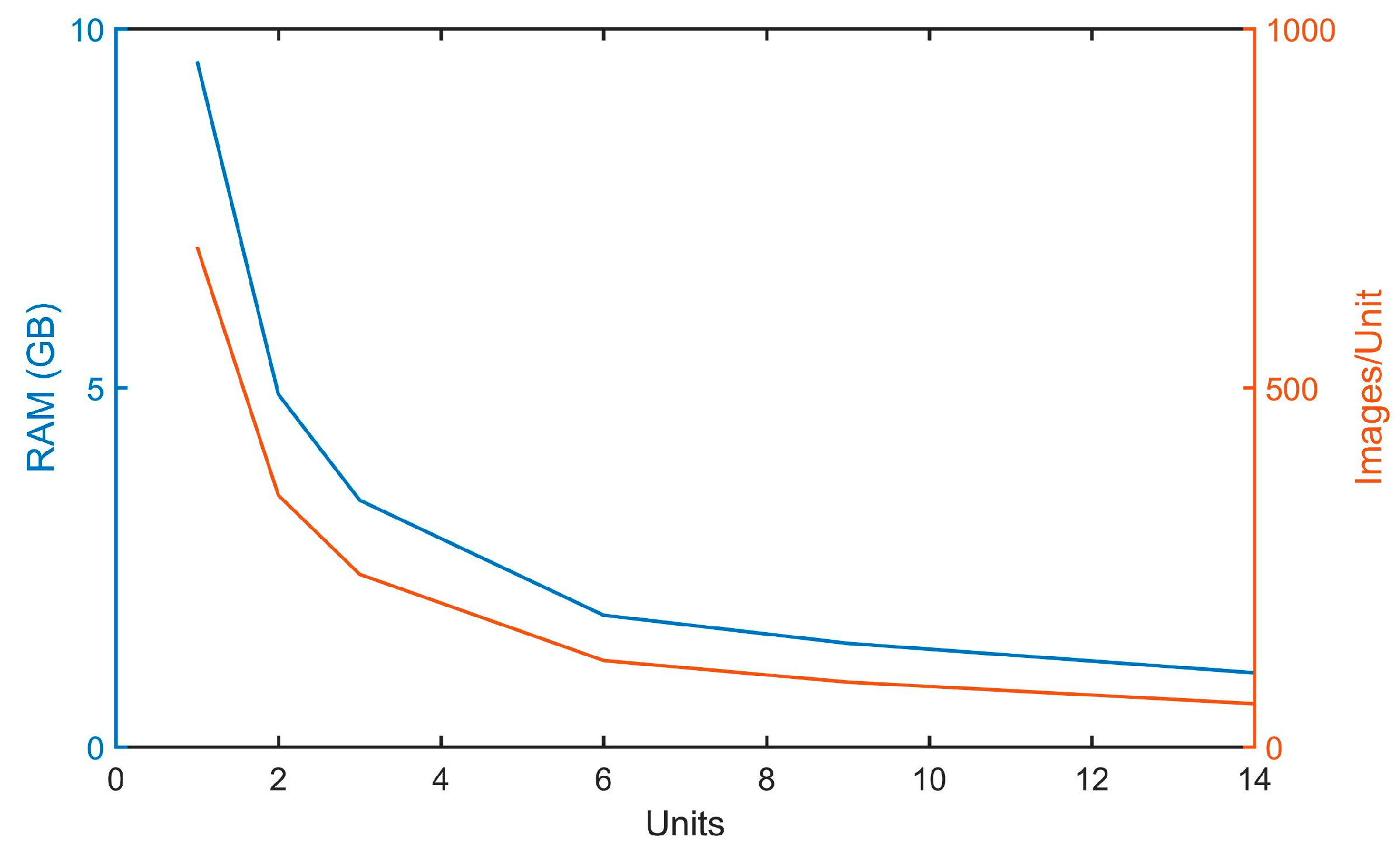
To demonstrate the efficiency of RT-GBSAR on the management of computational RAM, the entire dataset of 696 images used in the costal cliff case study was processed with different unit settings. The computational RAM, the number of units, and images per unit are summarized in Figure 12. The conventional processing of all the images together in one single unit required 9.5 GB (Gigabyte) RAM. The RAM was reduced to only 1.0 GB by the proposed RT-GBSAR with the setting of 14 units and 60 images per unit.
5. Conclusions
The significant challenges in processing continuous GBSAR data have been resolved through the implementation of the proposed RT-GBSAR chain. The chain has three notable features: (i) low requirement of computational RAM; (ii) insights into the evolution of surface movements through temporarily-coherent pixels; and (iii) real-time capability to process a theoretically infinite number of images. The applications of monitoring a fast-changing sand dune and a coastal cliff demonstrated that the proposed chain can achieve a precision of a few submillimeters in time series estimation. The dune application demonstrates the importance of vegetation in stabilizing coastal dune surfaces against sand erosion. In the coastal cliff application, the RT-GBSAR results reveal displacements only in the area near the sea and suggest that the triggering of ground deformation is related to the sea tides.
Author Contributions
Conceptualization, Z.W.; writing—original draft preparation, Z.W.; writing—review and editing, Z.W., Z.L. and J.M.; resources & data curation: Y.L., J.P. and S.L.; supervision, J.M. and Z.L.; funding acquisition, Z.L. and J.M.
Funding
This research was supported by a China Scholarship Council (CSC) studentship (No. 201506270153) held by Zheng Wang at Newcastle University, UK. Special gratitude goes to the Henry Lester Trust and the Great Britain–China Educational Trust (GBCET) for their financial support to Zheng Wang in his writing-up year. The work was also supported by the National Environment Research Council (NERC) through the 2014 Strategic Environmental Science Capital Investment (ref. CC049), the Centre for the Observation and Modelling of Earthquakes, Volcanoes, and Tectonics (COMET, ref. come30001), the LiCS project (ref. NE/K010794/1), by the European Space Agency through the ESA-MOST DRAGON-4 project (ref. 32244), and by the National Science Foundation of China (ref. 41877283 and ref. 41474014).
Conflicts of Interest
The authors declare no conflict of interest.
References
- Crosetto, M.; Monserrat, O.; Luzi, G.; Devanthéry, N.; Cuevas-González, M.; Barra, A. Data processing and analysis tools based on ground-based synthetic aperture radar imagery. ISPRS-Int. Arch. Photogramm. Remote Sens. Spat. Inf. Sci. 2017, 593–596. [Google Scholar] [CrossRef]
- Monserrat, O.; Crosetto, M.; Luzi, G. A review of Ground-Based sar interferometry for deformation measurement. ISPRS J. Photogramm. Remote Sens. 2014, 93, 40–48. [Google Scholar] [CrossRef]
- Caduff, R.; Schlunegger, F.; Kos, A.; Wiesmann, A. A review of terrestrial radar interferometry for measuring surface change in the geosciences. Earth Surf. Process. Landf. 2015, 40, 208–228. [Google Scholar] [CrossRef]
- Wang, Z.; Li, Z.; Mills, J. Modelling of instrument repositioning errors in discontinuous Multi-Campaign Ground-Based sar (mc-gbsar) deformation monitoring. ISPRS J. Photogramm. Remote Sens. 2019, 157, 26–40. [Google Scholar] [CrossRef]
- Crosetto, M.; Monserrat, O.; Luzi, G.; Cuevas-González, M.; Devanthéry, N. Discontinuous gbsar deformation monitoring. ISPRS J. Photogramm. Remote Sens. 2014, 93, 136–141. [Google Scholar] [CrossRef]
- Tarchi, D.; Antonello, G.; Casagli, N.; Farina, P.; Fortuny-Guasch, J.; Guerri, L.; Leva, D. On the use of ground-based sar interferometry for slope failure early warning: The cortenova rock slide (italy). In Landslides; Springer: Berlin/Heidelberg, Germany, 2005; pp. 337–342. [Google Scholar]
- Placidi, S.; Meta, A.; Testa, L.; Rödelsperger, S. Monitoring Structures with Fastgbsar. In Proceedings of the 2015 IEEE Radar Conference, Johannesburg, South Africa, 27–30 October 2015; IEEE: Arlington, VA, USA, 2015; pp. 435–439. [Google Scholar]
- Li, Z.; Fielding, E.J.; Cross, P. Integration of insar time-series analysis and water-vapor correction for mapping postseismic motion after the 2003 bam (Iran) earthquake. IEEE Trans. Geosci. Remote Sens. 2009, 47, 3220–3230. [Google Scholar]
- Ferretti, A.; Prati, C.; Rocca, F. Nonlinear subsidence rate estimation using permanent scatterers in differential sar interferometry. IEEE Trans. Geosci. Remote Sens. 2000, 38, 2202–2212. [Google Scholar] [CrossRef]
- Rödelsperger, S. Real-Time Processing of Ground Based Synthetic Aperture Radar (GB-SAR) Measurements. Ph.D. Thesis, Technische Universität Darmstadt, Fachbereich Bauingenieurwesen und Geodäsie, Darmstadt, Germany, 2011. [Google Scholar]
- Li, Y.; Jiao, Q.; Hu, X.; Li, Z.; Li, B.; Zhang, J.; Jiang, W.; Luo, Y.; Li, Q.; Ba, R. Detecting the slope movement after the 2018 baige landslides based on Ground-Based and Space-Borne radar observations. Int. J. Appl. Earth Obs. Geoinf. 2020, 84, 101949. [Google Scholar] [CrossRef]
- Caduff, R.; Wiesmann, A.; Bühler, Y.; Pielmeier, C. Continuous monitoring of snowpack displacement at high spatial and temporal resolution with terrestrial radar interferometry. Geophys. Res. Lett. 2015, 42, 813–820. [Google Scholar] [CrossRef] [Green Version]
- Iglesias, R.; Aguasca, A.; Fabregas, X.; Mallorqui, J.J.; Monells, D.; López-Martínez, C.; Pipia, L. Ground-Based polarimetric sar interferometry for the monitoring of terrain displacement Phenomena–Part i: Theoretical description. IEEE J. Sel. Top. Appl. Earth Obs. Remote Sens. 2015, 8, 980–993. [Google Scholar] [CrossRef]
- Roedelsperger, S.; Becker, M.; Gerstenecker, C.; Laeufer, G. Near Real-Time Monitoring of Displacements with the Ground Based Sar Ibis-L. In Proceedings of the International Workshop on ERS SAR Interferometry, Frascati, Italy, 30 November–4 December 2009. [Google Scholar]
- Wang, Z.; Li, Z.; Mills, J. A new approach to selecting coherent pixels for ground-based sar deformation monitoring. ISPRS J. Photogramm. Remote Sens. 2018, 144, 412–422. [Google Scholar] [CrossRef]
- Wang, Z.; Li, Z.; Mills, J. A new nonlocal method for ground-based synthetic aperture radar deformation monitoring. IEEE J. Sel. Top. Appl. Earth Obs. Remote Sens. 2018, 11, 3769–3781. [Google Scholar] [CrossRef]
- Hooper, A. A Statistical-Cost Approach to Unwrapping the Phase of INSAR Time Series. In Proceedings of the International Workshop on ERS SAR Interferometry, Frascati, Italy, 30 November–4 December 2009. [Google Scholar]
- Iannini, L.; Guarnieri, A.M. Atmospheric phase screen in Ground-Based radar: Statistics and compensation. IEEE Geosci. Remote Sens. Lett. 2011, 8, 537–541. [Google Scholar] [CrossRef]
- Pipia, L.; Fabregas, X.; Aguasca, A.; Lopez-Martinez, C. Atmospheric artifact compensation in Ground-Based dinsar applications. IEEE Geosci. Remote Sens. Lett. 2008, 5, 88–92. [Google Scholar] [CrossRef]
- Iglesias, R.; Fabregas, X.; Aguasca, A.; Mallorqui, J.J.; Lopez-Martinez, C.; Gili, J.; Corominas, J. Atmospheric phase screen compensation in Ground-Based sar with a Multiple-Regression model over mountainous regions. IEEE Trans. Geosci. Remote Sens. 2014, 52, 2436–2449. [Google Scholar] [CrossRef]
- Caduff, R.; Kos, A.; Schlunegger, F.; McArdell, B.W.; Wiesmann, A. Terrestrial radar interferometric measurement of hillslope deformation and atmospheric disturbances in the illgraben Debris-Flow catchment, switzerland. IEEE Geosci. Remote Sens. Lett. 2014, 11, 434–438. [Google Scholar] [CrossRef]
- Dong, Y.; Huang, D.; Du, J. Observations of coastal aeolian dune movements at feicuidao, on the changli gold coast in hebei province. Sci. Cold Arid Reg. 2013, 5, 0324–0330. [Google Scholar]
- NTSLF. The UK National Tidal Gauge Network. 2018. Available online: https://www.Ntslf.Org/data (accessed on 20 November 2018).
- Biggs, J.; Wright, T.; Lu, Z.; Parsons, B. Multi-Interferogram method for measuring interseismic deformation: Denali fault, alaska. Geophys. J. Int. 2007, 170, 1165–1179. [Google Scholar] [CrossRef]
- Usai, S. A least squares database approach for sar interferometric data. IEEE Trans. Geosci. Remote Sens. 2003, 41, 753–760. [Google Scholar] [CrossRef]
- Samiei-Esfahany, S.; Martins, J.E.; van Leijen, F.; Hanssen, R.F. Phase estimation for distributed scatterers in insar stacks using integer least squares estimation. IEEE Trans. Geosci. Remote Sens. 2016, 54, 5671–5687. [Google Scholar] [CrossRef]
- Ferretti, A.; Fumagalli, A.; Novali, F.; Prati, C.; Rocca, F.; Rucci, A. A new algorithm for processing interferometric Data-Stacks: Squeesar. IEEE Trans. Geosci. Remote Sens. 2011, 49, 3460–3470. [Google Scholar] [CrossRef]
Figure 1.
Schematic of the real-time ground-based synthetic aperture radar (RT-GBSAR) processing chain. SLC is single-look complex.
Figure 1.
Schematic of the real-time ground-based synthetic aperture radar (RT-GBSAR) processing chain. SLC is single-look complex.

Figure 2.
Flowchart of the small baseline subset (SBAS) time series analysis in the RT-GBSAR chain. APS is atmospheric phase screen.
Figure 2.
Flowchart of the small baseline subset (SBAS) time series analysis in the RT-GBSAR chain. APS is atmospheric phase screen.

Figure 3.
Overview of the sand dune at Feicuidao on the Changli Gold Coast, Hebei Province, China. (a) Oblique photograph of the site. Three in-situ corner reflectors (CRs) are marked with yellow circles. Two areas of interest are roughly outlined: Area #1 is covered with sparse vegetation and Area #2 is devoid of vegetation. (b) A corresponding amplitude image of this site.

Figure 4.
RT-GBSAR results of the sand dune dataset. (a–j): The displacement maps of all units from the first to the last, respectively. The cumulative displacement map with respect to units 3–6 is given in subfigure (k) and that of units 8–10 in (l). Note that Area #1 is indicated in a black loop and Area #2 in a red one.

Figure 5.
Sequential amplitude images during the period from 05:17:07 to 05:19:27.

Figure 6.
Overview of the coastal cliff. (a) Deployment of the FastGBSAR system for data collection. (b) Approximate co-registration of a GBSAR amplitude image with the planimetric view of the observing site in Google Earth.
Figure 6.
Overview of the coastal cliff. (a) Deployment of the FastGBSAR system for data collection. (b) Approximate co-registration of a GBSAR amplitude image with the planimetric view of the observing site in Google Earth.

Figure 7.
RT-GBSAR results of the coastal cliff dataset. (a–n): The displacement maps of all units from the first to the last are shown in subfigures, respectively. The cumulative displacement map with respect to pixels that are coherent over the entire observation period is given in (o).
Figure 7.
RT-GBSAR results of the coastal cliff dataset. (a–n): The displacement maps of all units from the first to the last are shown in subfigures, respectively. The cumulative displacement map with respect to pixels that are coherent over the entire observation period is given in (o).

Figure 8.
Tidal elevation for North Shields, Tynemouth, UK on 16 November 2016, obtained from the National Tidal and Sea Level Facility [23]. The variation of tidal elevation over the period of GBSAR observation is marked as red.
Figure 8.
Tidal elevation for North Shields, Tynemouth, UK on 16 November 2016, obtained from the National Tidal and Sea Level Facility [23]. The variation of tidal elevation over the period of GBSAR observation is marked as red.

Figure 9.
The time series of displacements and APS for the five selected pixels (P1, P2, P3, P4, and P5).
Figure 9.
The time series of displacements and APS for the five selected pixels (P1, P2, P3, P4, and P5).

Figure 10.
Precision maps for coherent pixels without unwrapping errors in the sand dune application. The precision maps for unit 1 to unit 10 are shown in subfigures (a–j), respectively. The precision map with respect to units 3–6 is given in subfigure (k) and that of units 8–10 in (l).
Figure 10.
Precision maps for coherent pixels without unwrapping errors in the sand dune application. The precision maps for unit 1 to unit 10 are shown in subfigures (a–j), respectively. The precision map with respect to units 3–6 is given in subfigure (k) and that of units 8–10 in (l).

Figure 11.
Precision maps for coherent pixels without unwrapping errors in the coastal cliff application. The precision maps for each unit from the 1st to the 14th are shown in subfigures (a–n), respectively. The precision map with respect to the total units 1–14 is given in subfigure (o).
Figure 11.
Precision maps for coherent pixels without unwrapping errors in the coastal cliff application. The precision maps for each unit from the 1st to the 14th are shown in subfigures (a–n), respectively. The precision map with respect to the total units 1–14 is given in subfigure (o).

Figure 12.
The number of units versus computational RAM and images per unit in RT-GBSAR.


Table 1.
Information about processing units of the sand dune dataset.
| Unit | Start | End | Coherent Pixels |
|---|---|---|---|
| 1 | 1 | 60 | 5085 |
| 2 | 51 | 110 | 3643 |
| 3 | 101 | 160 | 5222 |
| 4 | 151 | 210 | 5664 |
| 5 | 201 | 260 | 6128 |
| 6 | 251 | 310 | 6102 |
| 7 | 301 | 360 | 3298 |
| 8 | 351 | 410 | 4569 |
| 9 | 401 | 460 | 6887 |
| 10 | 451 | 478 | 6831 |
Table 2.
Information about processing units of the cliff dataset.
| Unit | Start | End | Coherent Pixels |
|---|---|---|---|
| 1 | 1 | 60 | 11,859 |
| 2 | 51 | 110 | 10,975 |
| 3 | 101 | 160 | 10,671 |
| 4 | 151 | 210 | 10,046 |
| 5 | 201 | 260 | 10,303 |
| 6 | 251 | 310 | 9273 |
| 7 | 301 | 360 | 9508 |
| 8 | 351 | 410 | 8887 |
| 9 | 401 | 460 | 8391 |
| 10 | 451 | 510 | 7503 |
| 11 | 501 | 560 | 6661 |
| 12 | 551 | 610 | 5691 |
| 13 | 601 | 660 | 4531 |
| 14 | 651 | 696 | 4331 |
Table 3.
Statistics with respect to unwrapping errors for the sand dune dataset.
| Unit | Coherent Pixels | Pixels without Unwrapping Errors (Percentage) | Pixels with Unwrapping Errors (Percentage) |
|---|---|---|---|
| 1 | 5085 | 5070 (99.71%) | 15 (0.29%) |
| 2 | 3643 | 3613 (99.18%) | 30 (0.82%) |
| 3 | 5222 | 5219 (99.94%) | 3 (0.06%) |
| 4 | 5664 | 5660 (99.93%) | 4 (0.07%) |
| 5 | 6128 | 6119 (99.85%) | 9 (0.15%) |
| 6 | 6102 | 6043 (99.03%) | 59 (0.97%) |
| 7 | 3298 | 3255 (98.70%) | 43 (1.30%) |
| 8 | 4569 | 4528 (99.10%) | 41 (0.90%) |
| 9 | 6887 | 6868 (99.72%) | 19 (0.28%) |
| 10 | 6831 | 6781 (99.27%) | 50 (0.73%) |
| 3–6 | 4030 | 4021 (99.78%) | 9 (0.22%) |
| 8–10 | 3712 | 3690 (99.41%) | 22 (0.59%) |
Table 4.
Statistics with respect to unwrapping errors for the cliff dataset.
| Unit | Coherent Pixels | Pixels without Unwrapping Errors (Percentage) | Pixels with Unwrapping Errors (Percentage) |
|---|---|---|---|
| 1 | 11,859 | 11,857 (99.98%) | 2 (0.02%) |
| 2 | 10,975 | 10,973 (99.98%) | 2 (0.02%) |
| 3 | 10,671 | 10,668 (99.97%) | 3 (0.03%) |
| 4 | 10,046 | 10,032 (99.86%) | 14 (0.14%) |
| 5 | 10,303 | 10,297 (99.94%) | 6 (0.06%) |
| 6 | 9273 | 9272 (99.99%) | 1 (0.01%) |
| 7 | 9508 | 9506 (99.98%) | 2 (0.02%) |
| 8 | 8887 | 8868 (99.79%) | 19 (0.21%) |
| 9 | 8391 | 8388 (99.96%) | 3 (0.04%) |
| 10 | 7503 | 7502 (99.99%) | 1 (0.01%) |
| 11 | 6661 | 6659 (99.97%) | 2 (0.03%) |
| 12 | 5691 | 5691 (100.00%) | 0 (0.00%) |
| 13 | 4531 | 4531 (100.00%) | 0 (0.00%) |
| 14 | 4331 | 4331 (100.00%) | 0 (0.00%) |
| 1–14 | 3428 | 3421 (99.80%) | 7 (0.20%) |
Table 5.
Real-time capability and time-series results for different sets of parameters.
| W | T (Δt) | Overlap: 2T (Δt) | Ifgs 1/Unit | Units | CPs 2 | L 3 | Errors 4 | RMS 5 (mm) | Total ifgs | TW (Δt) | TP (s) |
|---|---|---|---|---|---|---|---|---|---|---|---|
| 5 | 1 | 2 | 4 | 33 | 1826 | 0 | NA | NA | 131 | 3 | 101 |
| 10 | 1 | 2 | 9 | 9 | 2122 | 0 | NA | NA | 111 | 8 | 56 |
| 15 | 1 | 2 | 14 | 8 | 2264 | 0 | NA | NA | 106 | 13 | 48 |
| 20 | 1 | 2 | 19 | 6 | 2319 | 0 | NA | NA | 104 | 18 | 41 |
| 5 | 2 | 4 | 7 | 94 | 2194 | 98 | 0 | 0.33 | 662 | 1 | 329 |
| 10 | 2 | 4 | 17 | 16 | 2997 | 98 | 0 | 0.38 | 272 | 6 | 77 |
| 15 | 2 | 4 | 27 | 9 | 3229 | 98 | 0 | 0.4 | 237 | 11 | 72 |
| 20 | 2 | 4 | 37 | 6 | 3410 | 98 | 0 | 0.44 | 222 | 16 | 62 |
| 5 | 3 | NA | NA | NA | NA | NA | NA | NA | NA | NA | NA |
| 10 | 3 | 6 | 24 | 23 | 3166 | 292 | 0 | 0.27 | 558 | 4 | 144 |
| 15 | 3 | 6 | 39 | 11 | 3673 | 292 | 1 | 0.3 | 414 | 9 | 110 |
| 20 | 3 | 6 | 54 | 7 | 3691 | 292 | 0 | 0.31 | 366 | 14 | 93 |
| 5 | 4 | NA | NA | NA | NA | NA | NA | NA | NA | NA | 386 |
| 10 | 4 | 8 | 30 | 44 | 3175 | 580 | 0 | 0.19 | 1336 | 2 | 163 |
| 15 | 4 | 8 | 50 | 13 | 3670 | 580 | 7 | 0.23 | 654 | 7 | 151 |
| 20 | 4 | 8 | 70 | 8 | 3972 | 580 | 6 | 0.26 | 544 | 12 | 101 |
1 Ifgs: interferograms; 2 CPs: coherent pixels over all units; 3 L: the number of closed temporal loops; 4 Errors: coherent pixels with unwrapping errors; 5 RMS: precision indicator for time series estimation.
© 2019 by the authors. Licensee MDPI, Basel, Switzerland. This article is an open access article distributed under the terms and conditions of the Creative Commons Attribution (CC BY) license (http://creativecommons.org/licenses/by/4.0/).
Share and Cite
MDPI and ACS Style
Wang, Z.; Li, Z.; Liu, Y.; Peng, J.; Long, S.; Mills, J. A New Processing Chain for Real-Time Ground-Based SAR (RT-GBSAR) Deformation Monitoring. Remote Sens. 2019, 11, 2437. https://0-doi-org.brum.beds.ac.uk/10.3390/rs11202437
AMA Style
Wang Z, Li Z, Liu Y, Peng J, Long S, Mills J. A New Processing Chain for Real-Time Ground-Based SAR (RT-GBSAR) Deformation Monitoring. Remote Sensing. 2019; 11(20):2437. https://0-doi-org.brum.beds.ac.uk/10.3390/rs11202437
Chicago/Turabian StyleWang, Zheng, Zhenhong Li, Yanxiong Liu, Junhuan Peng, Sichun Long, and Jon Mills. 2019. "A New Processing Chain for Real-Time Ground-Based SAR (RT-GBSAR) Deformation Monitoring" Remote Sensing 11, no. 20: 2437. https://0-doi-org.brum.beds.ac.uk/10.3390/rs11202437
Note that from the first issue of 2016, this journal uses article numbers instead of page numbers. See further details here.