1. Introduction
Crop growth condition monitoring is critical to decision making in both public and private sectors that concern agricultural policy, production, food security, and food prices. Remotely sensed data have been used for crop growth monitoring for a long time [
1,
2,
3,
4,
5,
6,
7]. The Normalized Difference Vegetation Index (NDVI) has been widely used for research and operations of crop condition assessment [
8,
9,
10,
11,
12,
13]. NDVI changes dynamically with crop biomass changing from its emergence to maturity [
14,
15,
16]. It has become the indicator for crop growth condition monitoring [
12,
13,
14,
15,
16,
17]. For the same crop at the same growth stage, the higher NDVI value usually indicates better vegetation condition, i.e., better crop (growth) condition.
Traditionally, crop NDVIs of different years, especially two adjacent years, matched on calendar day were compared at pixel scale [
12]. The crop growth conditions were compared with the assumption that the crops were at the same growing stage. However, this assumption is often violated in real-world [
17,
18]. Crops aligned with the calendar for comparison are often at different growing stages with a time variation from 1–2 days to even more than 10 days depending on crop, weather, and geolocation [
19]. Therefore, the assessment results based on the matched calendar are not reliable. The better/worse vegetation condition might actually indicate the delayed or earlier development of the crop growing stages in the compared year.
In general, traditional crop growth condition assessment was based on pixel level NDVI comparison. For a given pixel, the crops planted in the different years might be different. Therefore, comparing the NDVIs of different years at pixel level may result in a comparison of NDVIs of different types of crops. The traditional method is thus not suitable for crop specific growth condition assessment. To overcome this problem, this paper proposed to aggregate crop specific pixels into area of interest and derive zonal statistics, such as county average for crop condition assessment.
Moreover, in crop growth condition assessment, multi-day composite remote sensing products rather than daily remotely sensed data are often used to reduce the image noise, such as cloud, haze, and dust. This practice often introduces extra uncertainty in the crop growth condition assessment. However, real-time monitoring based on daily remotely sensed data is desperately needed, especially for fast growing period. The crop conditions change rapidly and are difficult to capture by using the multi-day composite NDVI time-series. In addition, US Department of Agriculture (USDA), National Agricultural Statistics Service (NASS) is mandated to provide a weekly Crop Progress and Condition report. The available composite NDVI data product, such as NASA 8-day NDVI composite has difficulty meeting the NASS’s needs for weekly reports.
Daily remotely sensed data can deliver more accurate and near real-time monitoring results. However, it suffers cloud contamination, noise, and massive data processing capability requirements. Therefore, the daily surface reflectance MODIS data at 250 m spatial resolution are used and a filtering process is applied in this study to produce NDVI time series for crop vegetation condition assessment. Furthermore, there has been no effective method yet that can assess crop growth conditions at a given time for a specific crop growing stage from the remotely sensed data. Obviously, crop growth stage estimation is critical for a more detailed and accurate crop growth condition assessment based on remotely sensed data.
In continued efforts, many researchers used the modeled time series remotely sensed data to produce the crop phenology for real-time crop progress monitoring [
20,
21,
22,
23]. However, most research extracted the crop growth stages using the remotely sensed data based on either a predefined VI threshold or the inflection points of the fitting function [
21,
22,
23]. The crop growth stages derived from those approaches usually have long intervals, identifying only coarse growth stages of corn such as corn emergence, greenup, silking, and maturity. More detailed short-interval growth stages, such as six leaves fully emerged (growing point above soil), eight leaves fully emerged (tassel beginning to develop), 10 leaves fully emerged (rapid growth phase begins), etc., cannot be extracted because there is no big inflection change in the vegetation index curve among these short-interval stages.
To estimate the short-interval growth stages effectively, another method based on daily air temperature data was adapted for crop growth stage estimation in this paper. Crops require a certain amount of heat energy to reach a specific growth stage, regardless of the number of calendar days taken [
24,
25,
26]. Crops grow from one growth stage to the next, in absence of extreme conditions such as unseasonal drought or disease, when it absorbs a certain amount of needed heat after planting. The heat that it receives can be quantitatively measured by air temperature accumulation, such as active accumulated temperature (AAT) or Growing Degree Unit (GDU). Thus, the corn growth stages can be identified to a precise date with the AAT time series that are precisely correlated with corn progress [
27]. The corn growth conditions are thus enabled to be assessed based on growth stages.
The purpose of this study is to develop a method for county scale corn (crop specific) growth condition assessment based on heat-aligned growth stages. Specifically, this study will investigate (1) whether the specific crop growth stage estimated from AAT time series data is consistent with NASS reporting; (2) whether the filtering process combining the Best Index Slope Extraction (BISE) and Savitzky–Golay filters works well for the NDVI time series derived from the daily surface reflectance MODIS data with 250 m spatial resolution; and (3) whether assessing corn growth conditions with respect to the growth stages is more reliable than that aligned on Julian days.
This paper is organized as follows.
Section 1 introduces background and the problem to be addressed.
Section 2 describes materials including the study area and experimental data used in this study.
Section 3 describes the methodology details and test scenarios for this study.
Section 4 presents experimental results.
Section 5 further discusses some issues about method, results and data, and future work. Finally,
Section 6 summarizes findings and conclusions.
2. Materials
2.1. Study Area
Corn is one of the major crops produced in the United States and the State of Iowa is one of the major corn-planting states. Carroll County located in central west Iowa was selected as the study area as shown in
Figure 1. Carroll County has about 365,000 acres of land, about 23,600 MODIS pixels. About half of the land cover pixels (about 11,800) are corn pixels. The corn and soybean have a regular rotation, but its planting acreages do not change dramatically every year. The dimensions of farm fields in Carroll County range from 250 m to 1 km. Most of the fields are around 500 × 500 or bigger. After excluding mixed pixels (MODIS size), which has less than 90% corn coverage, we still had adequate corn coverage for analysis.
2.2. Materials
2.2.1. MODIS Data
MODIS daily surface reflectance data MOD09GQ (with 250 m spatial resolution) from 2007 to 2017 covering corn growing season (from April 1 to October 31) were used for crop growth condition assessment. The version 6 MOD09GQ.006 were downloaded at website (
https://e4ftl01.cr.usgs.gov). Tile h10v04 and tile h11v04 covering the study area were downloaded and mosaicked using the MODIS Re-projection Tool (MRT). The daily NDVIs were calculated from the whole mosaicked MOD09GQ image and time series of NDVI subset of Carroll County were produced every year.
2.2.2. Cropland Data Layer (CDL)
The National Agricultural Statistics Service (NASS) of the US Department of Agriculture (USDA) produced a raster-formatted, geo-referenced, crop-specific land cover map named the Cropland Data Layer (CDL) [
28]. CDL provides annual crop type information at pixel level. The previous year CDL is usually released in the following year to the general public. The CDL data are freely available from USDA/NASS website or NASS’s web GIS application CropScape (
https://nassgeodata.gmu.edu/CropScape/) [
29]. The CDL data of Carroll County, Iowa from 2007 to 2017 were downloaded for extracting the corn crop layer for every year. The extracted corn data layer was used as a crop mask to calculate the corn crop NDVI mean of Carroll County and to produce its corn growing curve (corn phenology) afterwards. The CDL products from 2008 to 2017 were generated with 30-m resolution based on Landsat 5/7 imagery, while the CDL in 2007 was based on the Advanced Wide Field Sensor (AWiFS) on IRS-P6 with 56-m resolution. In the State of Iowa, the overall classification accuracies for major crops (soybeans and corn) from 2001 to 2014 were generally above 96% [
28].
2.2.3. Daymet Data
Daymet is a data product derived with a collection of algorithms and computer software designed to interpolate and extrapolate from daily meteorological observations to produce gridded estimates of daily weather parameters [
30]. The Daymet daily weather data with 1-km resolution was selected in this study for its convenience and availability. The data were downloaded from
https://daymet.ornl.gov. The Daymet dataset provides 1 × 1 km gridded estimates of daily weather parameters for North America, including daily continuous surfaces of minimum and maximum temperature, precipitation occurrence and amount, humidity, shortwave radiation, snow water equivalent, and day length. Archived and distributed through the Oak Ridge National Laboratory (ORNL) Distributed Active Archive Center (DAAC), Daymet data are available from 1980 through the latest full calendar year and includes the United States, Mexico, Canada, Hawaii, and Puerto Rico. The daily maximum and minimum temperature data from 2007 to 2017 covering the same period as MODIS data were extracted and processed to produce the daily average temperature of the study area.
3. Methodology
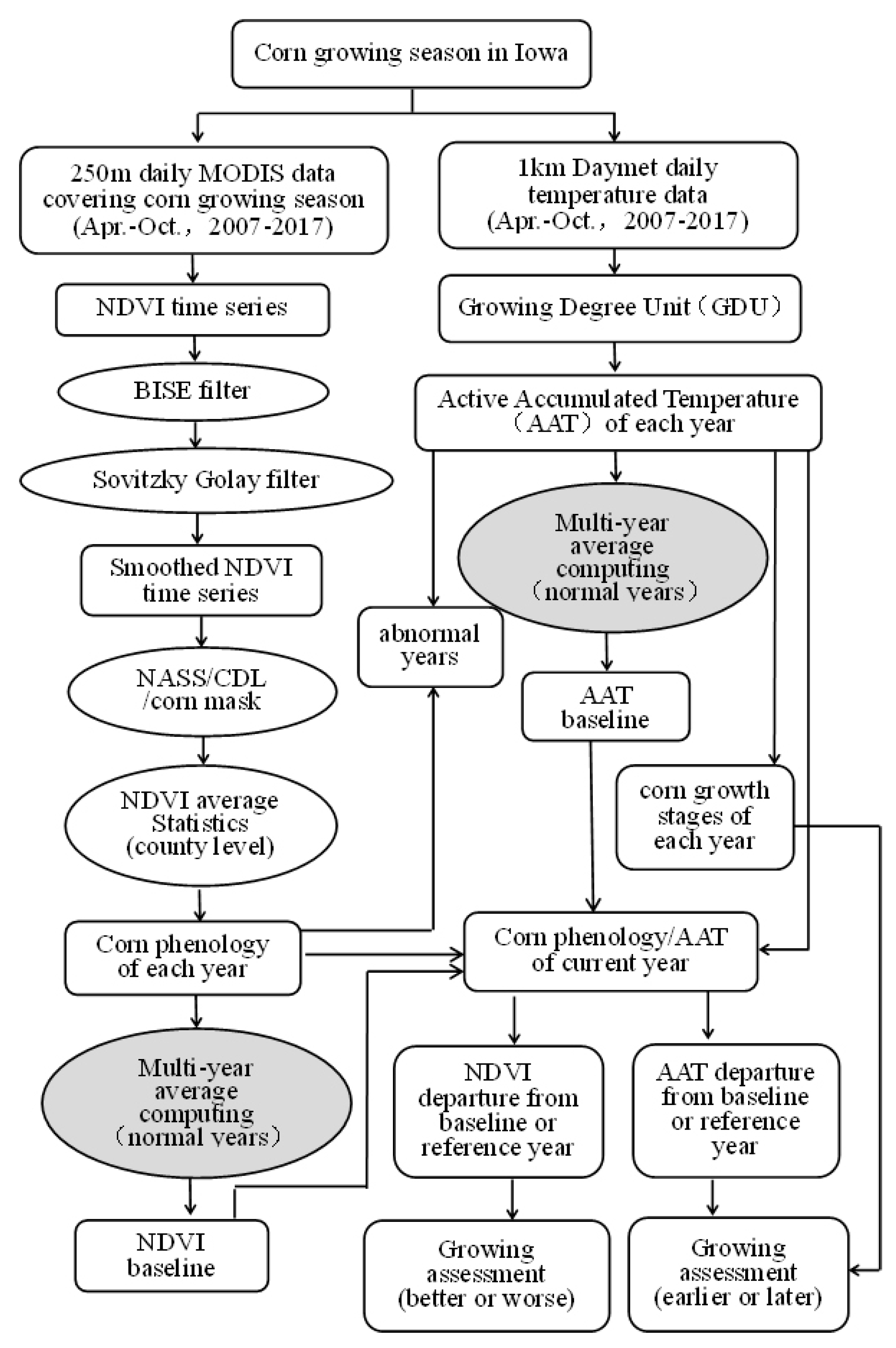
To assess corn growth conditions with respect to the growth stages, we have to solve two major issues. One is to filter the MODIS NDVI noise to reconstruct daily NDVI time series. The other is to estimate the corn growth stages based on the active accumulated temperature.
Figure 2 illustrates the overall workflow of procedures for filtering the MODIS data noise, constructing NDVI time series, computing AAT, estimating the corn growth stages, and assessing crop growth conditions based on aligned crop growth stages. The following subsections will present the data processing procedures in detail.
3.1. NDVI Noise Reduction and Corn Phenology Construction
As shown in
Figure 2, the daily MODIS NDVI data of corn growing season from 2007 to 2017 were first calculated from 250 m MOD09GQ daily data and NDVI time series of each year was produced. As shown in
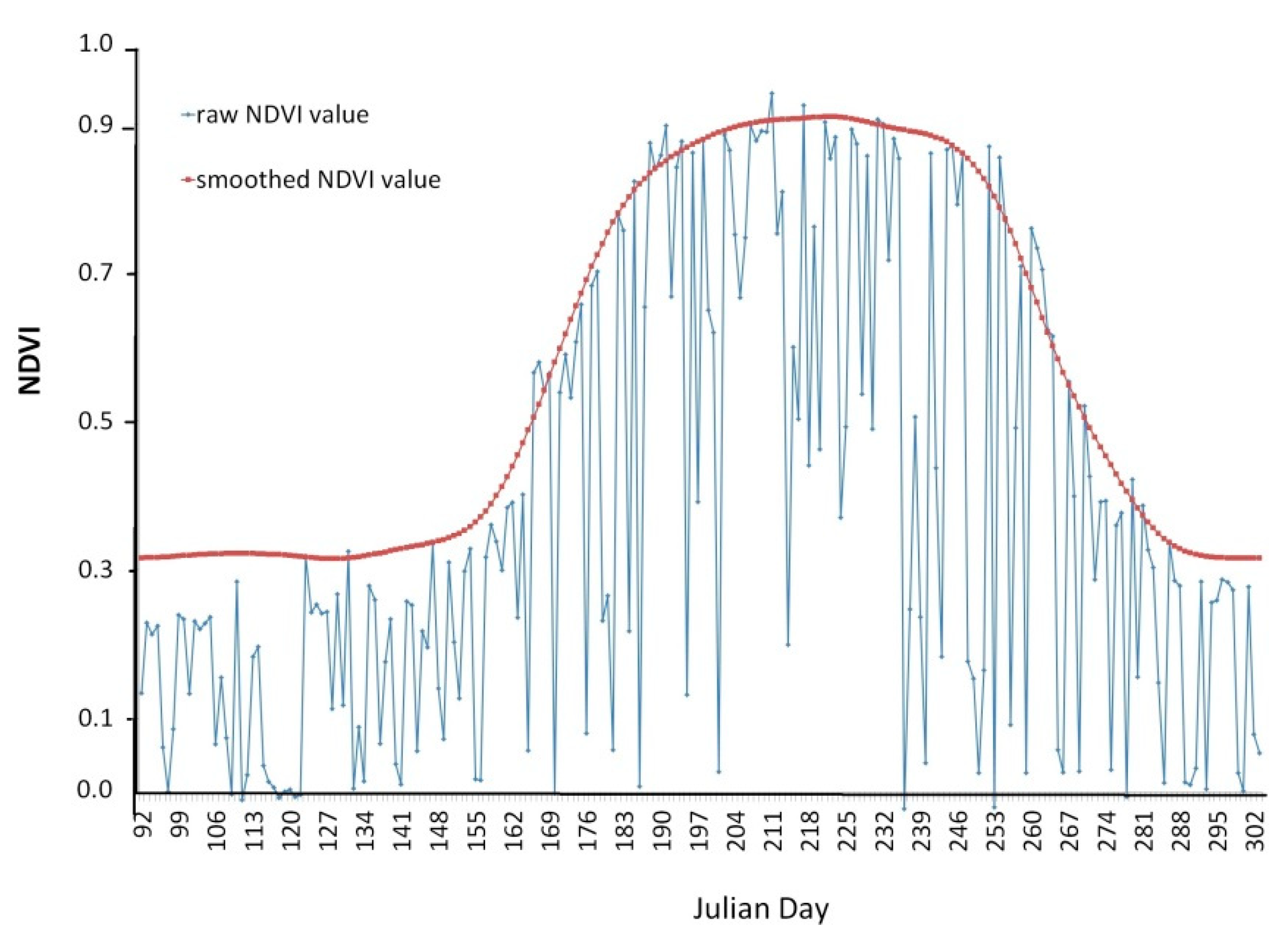
Figure 3, the typical raw NDVI curve of the corn growing season is greatly distorted by the noises from atmospheric conditions, sensor viewing geometry, and other factors. A temporal filtering and smoothing process has to be applied to eliminate the noise before the NDVI data can be used to assess the corn growth condition.
Many methods have been studied to eliminate the remote sensing image noise and to reconstruct NDVI time series. Noise filtering and NDVI reconstruction methods can be grouped into four categories: threshold-based, Fourier-based fitting, asymmetric function fitting, and iterative simple mathematical operation [
31]. Rahman et al. compared several methods to reduce the NDVI noise and found that the combination of Best Index Slope Extraction (BISE) and Savitzky–Golay filter yielded the best result [
32]. Thus, this paper adopts the combined filtering method, in which BISE is used as the first step filter to extract the best possible NDVI values and then Savitzky–Golay filter is used as the second step filter to smooth the NDVI time series by interpolating values selected from the first step. The filtered NDVI time series data, as shown in red in
Figure 3, shows that the noise was significantly reduced, and the cloud contaminated pixels were effectively reconstructed. The reconstructed NDVI time series curve is much smoother and fits the envelop well especially during the main crop growing season, which makes it possible to compare NDVI (i.e., the crop growth condition) at daily scale for further crop growth condition assessment.
From the reconstructed NDVI time series, the corn NDVI curve time series of each year can be easily derived using the corn crop mask and aggregated at county level. The smoothed MODIS NDVI data were first reprojected into the same projection as the CDL data: Albers Conical Equal Area projection. The corn field pixels were first identified from NASS’s Cropland Data Layer [
28,
29] as a corn crop mask for Carroll County. The corn crop mask was then used to extract the MODIS corn pixels of NDVI time series of each year. In the study, a MODIS pixel is considered as a corn pixel if 90% of the pixel is covered by 30 m resolution corn pixels taking into account road, trees, or other factors in the pixel. The daily NDVI spatial average was computed from the extracted corn MODIS pixels for Carroll County. The yearly NDVI spatial average time series from 92th Julian day to 303th Julian day (i.e., April 1 to October 30) were produced for each year from 2007 to 2017, as shown in
Figure 4.
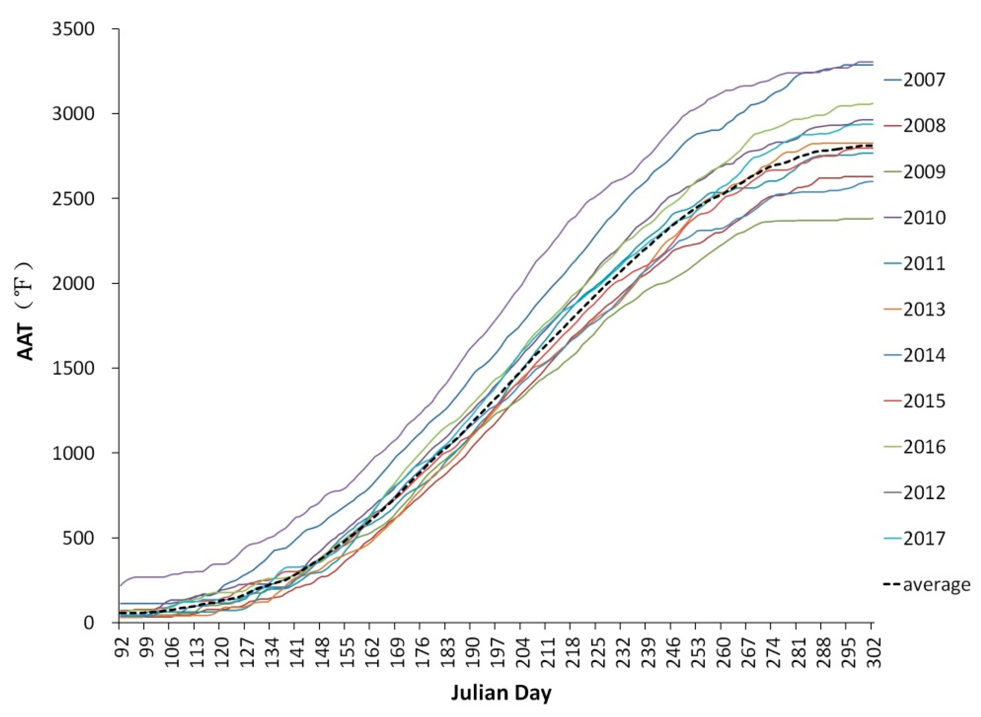
For crop condition comparison, past multi-year yearly NDVI spatial average time series were averaged to produce a baseline (reference) county average NDVI time series. As observed in
Figure 4, the corn phenology of the year 2012 is significantly different from other years due to large scale drought in the US Midwestern area. This abnormal year was excluded in the multi-year average computing. Therefore, nine years of county average NDVI data from 2007 to 2016 excluding 2012 were used to compute the average NDVI value as a normal reference (i.e., NDVI baseline). The year 2017 NDVI data was used as a current study year for assessment and validation.
Uncertainty Assessment
The processes for filtering and smoothing MODIS NDVI data are complicated. There are always errors associated with the processed data. Uncertainties always exist. The Carroll County has about 23,600 MODIS pixels. About half of land cover pixels (about 11,800) are corn pixels. Any statistics derived from this large number of samples are of significant statistical meaning.
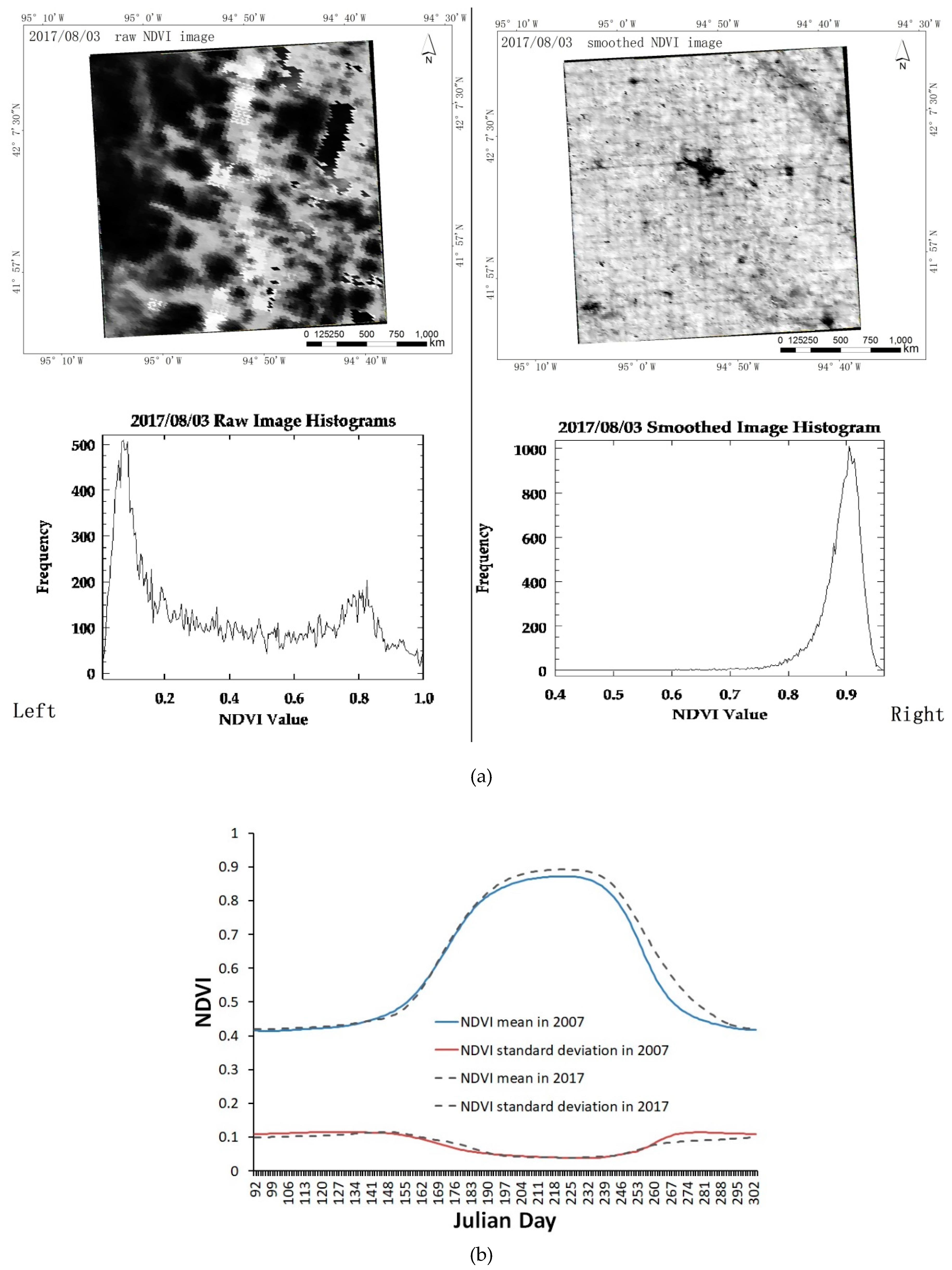
Figure 5a illustrates the difference between the original data and the noise-removed reconstructed data on August 3, 2017 (Julian date 215), and their pixel value histograms. The histogram shown on lower right of
Figure 5a shows that most of pixels center around NDVI value 0.9. This is consistent with the NDVI values around Julian date 215 in
Figure 3. Please note that the histogram includes all pixels in the county, and most of land cover is crop cover. For the corn only pixels, the histogram will be tighter (smaller variance).
To assess the spatial and temporal uncertainties, the standard deviations of the smoothed county corn NDVIs of two growing seasons were computed as shown in
Figure 5b. The standard deviations of NDVIs vary from 4% to 27% of their means during the corn growing season. The biggest NDVI variations happened in emergence and senescence periods. This is expected as planting dates vary and harvesting time vary from farm to farm. The planting and harvesting differences will affect vegetation significantly. However, in most of the growing period, the NDVI variations are relatively small, and have less uncertainty. This indicates that the crop condition assessments based on the averaged NDVI values are robust with small uncertainty. Of course, there is always spatial variation. However, this study focuses on the county level assessment, in which the assessment variables are all aggregated. The sub county spatial variation is averaged out. The county level spatial variation will be captured by individual county assessment.
3.2. Growing Degree Unit (GDU) and AAT Calculation
Neild and Newman indicated that every different development stage of corn, after planting, could be identified by the different accumulated temperatures calculated with growing degree unit (GDU) [
27]. The AAT and GDU, as a heat energy measure, have been widely used to identify the growth stages of crops such as corn and soybean [
33,
34,
35]. GDU is calculated based on daily air temperature (from Daymet data [
30]) as defined in Equation (1) [
34,
36]:
where
Tmax and
Tmin represent daily maximum and minimum air temperatures respectively, and
Tbase is the base temperature below which plants do not grow or grow very slowly.
Tbase varies among species and possibly cultivars, and likely varies with growth stage being considered [
36]. In Equation (1), 10 °C (50 °F) is usually used as the base temperature
Tbase for corn [
37,
38,
39,
40]. However, the corn crop will be stressed to even stop growing when the temperature is above 30 °C (86 °F) [
40,
41]. When the
Tmax or
Tmin is above 30 °C, they will be reset equal to 30 °C; and when they are below 10 °C, they will be reset equal to the
Tbase as shown in Equations (2) and (3) [
42]. The upper threshold temperature of 30 °C (86 °F) is not taken into account for crop condition assessment since it usually occurs in the later growth stage of corn and mainly affects the corn reproductive growth and its yield rather than the biomass (growth condition indicator).
When GDUs are calculated, the AAT time series can be derived by summing up day by day as given by Equation (4). The AAT time series {
AAT} is given by Equation (5).
where
i represents the
ith day after corn planting and
n means the last day to be counted. The active accumulated temperature
AATi provides an objective measure of how much heat corn received from the planting day to any given
ith day in the growing season.
To compare the general heat conditions in different years, especially in the corn seeding period and early growth stage, AAT is calculated from the first Julian calendar day of each year in this paper. In this case,
AAT1 in Equation (5) represents the AAT value of the first Julian day of each year rather than that of the corn planting day. However, the AAT value is zero until the daily mean temperature rises above 10 °C in the Spring months. From the AAT time series, an AAT curve is produced at county level, as shown in
Figure 6. The daily GDUs and AAT time series are calculated for the entire corn growing season from the April 1 to October 30 for each year from 2007 to 2017 in this study. The multi-year average AATs (the black dashed line, as shown in
Figure 6) was calculated as a normal reference (baseline) in the same way as the NDVI baseline, which was the arithmetic mean value of all the years excluding the abnormal year of 2012.
3.3. Corn Growth Stage Estimation Based on GDU and AAT
With adequate moisture and soil temperatures above 50 °F (i.e., GDU > 0), the radicle will begin to elongate from the corn seed [
34,
35] (to make it more readable, all temperature units will use Fahrenheit degree measure from now on). Therefore, the temperature 50 °F (or GDU > 0) is used as the suitable temperature for corn planting. The potential planting date can thus be traced from the GDUs during the seeding period. In this paper, the corn planting day
DATEplant is defined as the fifth day of the first period in which the air temperature lasts 5 days above 50 °F. With a known planting date
DATEplant, the AAT value change (
ΔAATplant_S) from crop planting day to the day that reaches the current growth stage
S can be derived from the following Equation (6).
where
AATS is the AAT value calculated from the first Julian day to the day when corn reaches the current growth stage
S,
AATplant is the AAT from the first Julian day to the day when corn is planted (this value is set zero if AAT calculation started from the planting day).
AATS and
AATplant correspond to two specific dates
DATES and
DATEplant, respectively. Neild and Newman found the Δ
AATplant_S needed for every growth stage after corn planting, as shown in
Table 1 [
27] (they called Δ
AAT as GDD in their paper). Therefore, every growth stage
DATES can be found by matching the Δ
AATplant_S in the table. The day that the matching Δ
AATplant_S is found is
DATES. Usually, Δ
AATplant_S will fall in a bracket of two consecutive stages. The earlier stage is identified as the current stage.
3.4. Corn Growth Condition Assessment
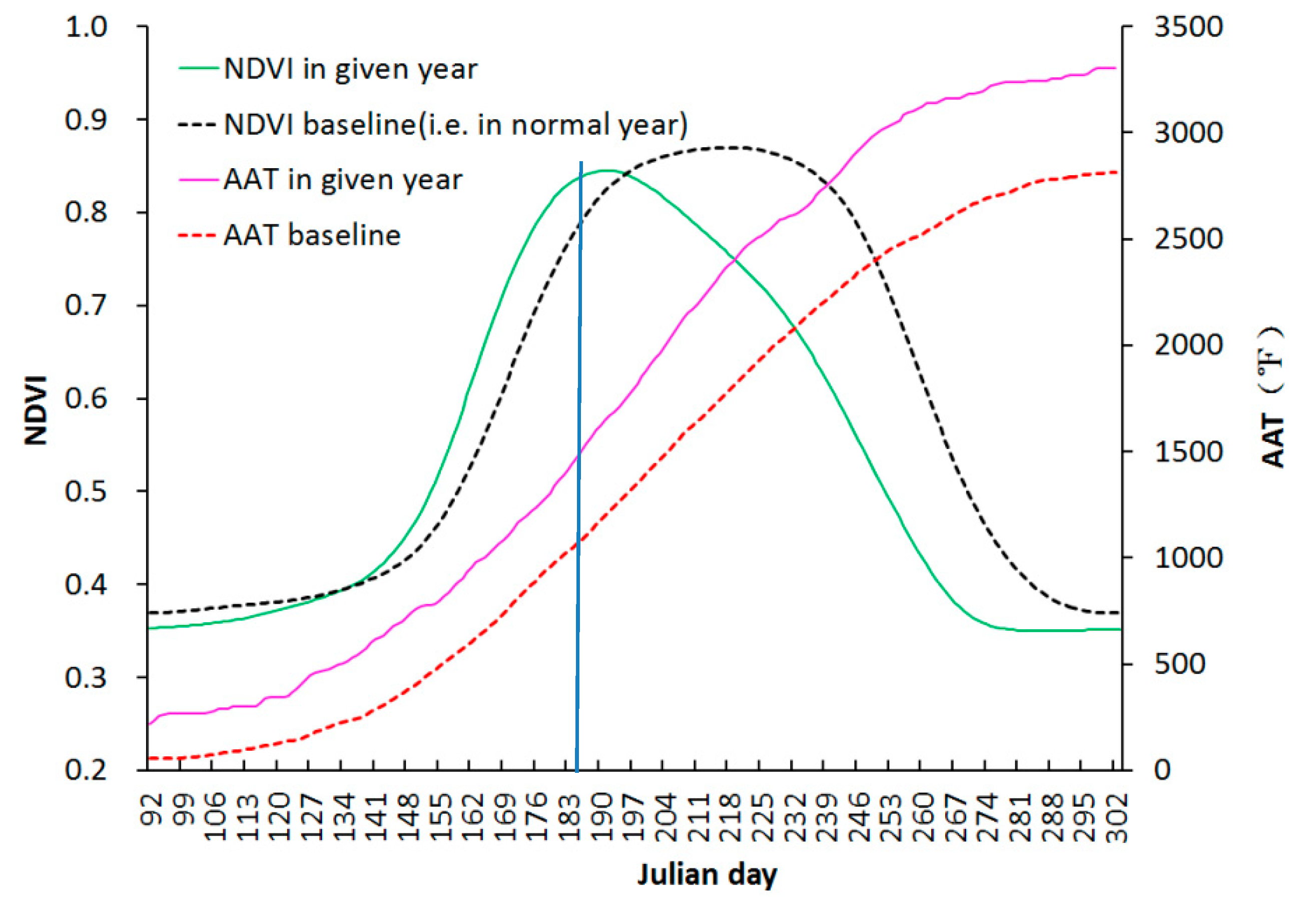
To measure the corn vegetation growth condition, the NDVI values are used after its emergence. The NDVIs of the same type of crops between two different years are usually different, as shown in
Figure 7, due to different soil moisture and heat conditions such as the AAT variations. Obviously, if NDVIs are compared based on the same Julian day, it is difficult to have a fair assessment of the crop growth condition for the given year due to crop development stage misalignment. To measure the corn growth condition, the NDVI values are used after its emergence. The NDVI’s deviation from the baseline represents the difference of corn growth condition between the study year and a baseline. Similarly, the current year AAT’s deviation from the baseline can quantify the difference of the days reaching a specific corn growth stage between the current year and the reference year.
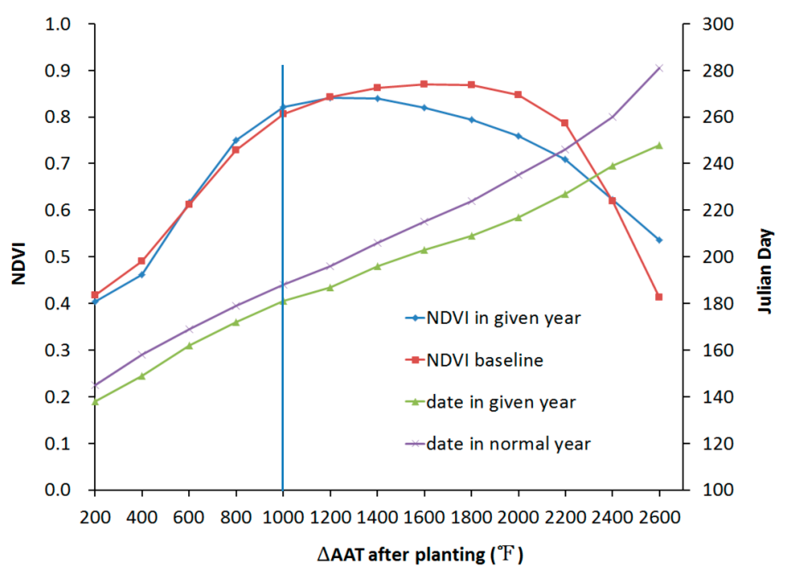
Therefore, this paper proposes to assess the NDVI’s departure from the baseline by aligning crop growth stages of the current year and normal year (baseline) using ΔAAT, as described in
Section 3.3. The NDVIs on different Julian dates but on the same growth stages are compared. The same crop growth stages are matched with the same or closest ΔAAT value after crop planting, as shown in
Figure 8. With the alignment of the growth stages, the NDVI can be compared with a traditional comparison model as given by Equation (7).
where Δ
NDVI is the NDVI deviation from the normal (reference) year; and
NDVIg and
NDVIb are NDVI values of the given study year and normal year (baseline), respectively. If Δ
NDVI is positive (or negative), it suggests that the crop growth condition in the given year is better (or worse) than the baseline. The absolute value of Δ
NDVI indicates the NDVI deviation from the baseline, or the magnitude of the crop growth condition better or worse than the normal year based on the same growth stage.
4. Results
In this study, the corn growth conditions assessment were tested both on the aligned growth stages and the aligned Julian days. The study results were validated with the NASS published Weekly Crop Progress and Condition Report.
4.1. Corn Growth Stage Estimation
As shown in
Table 2, every corn growth stage identified in Julian day in Carroll County from year 2011 to 2017 was derived from
Table 1 and the ΔAATs calculated from the corn planting date (Julian day). The five-year averages were calculated as the baseline for reference. The potential corn planting day of the five-year average is the median date of the previous five years.
Table 2 lists the ΔAAT-aligned corn growth stages in Carroll County from 2012 to 2017. The first column in the table lists the different growth stages of corn. The numbers in the right columns represent the Julian dates when corn reaches the different stages in different years. As shown in
Table 2, in the year 2012 the corn planting date is on Julian day 122, which is almost on the normal planting date (the five-year-average planting date is on Julian day 123), while in year 2013 corn planting date is on Julian day 138, which is much later than the normal planting date (about two weeks later than 5yr average).
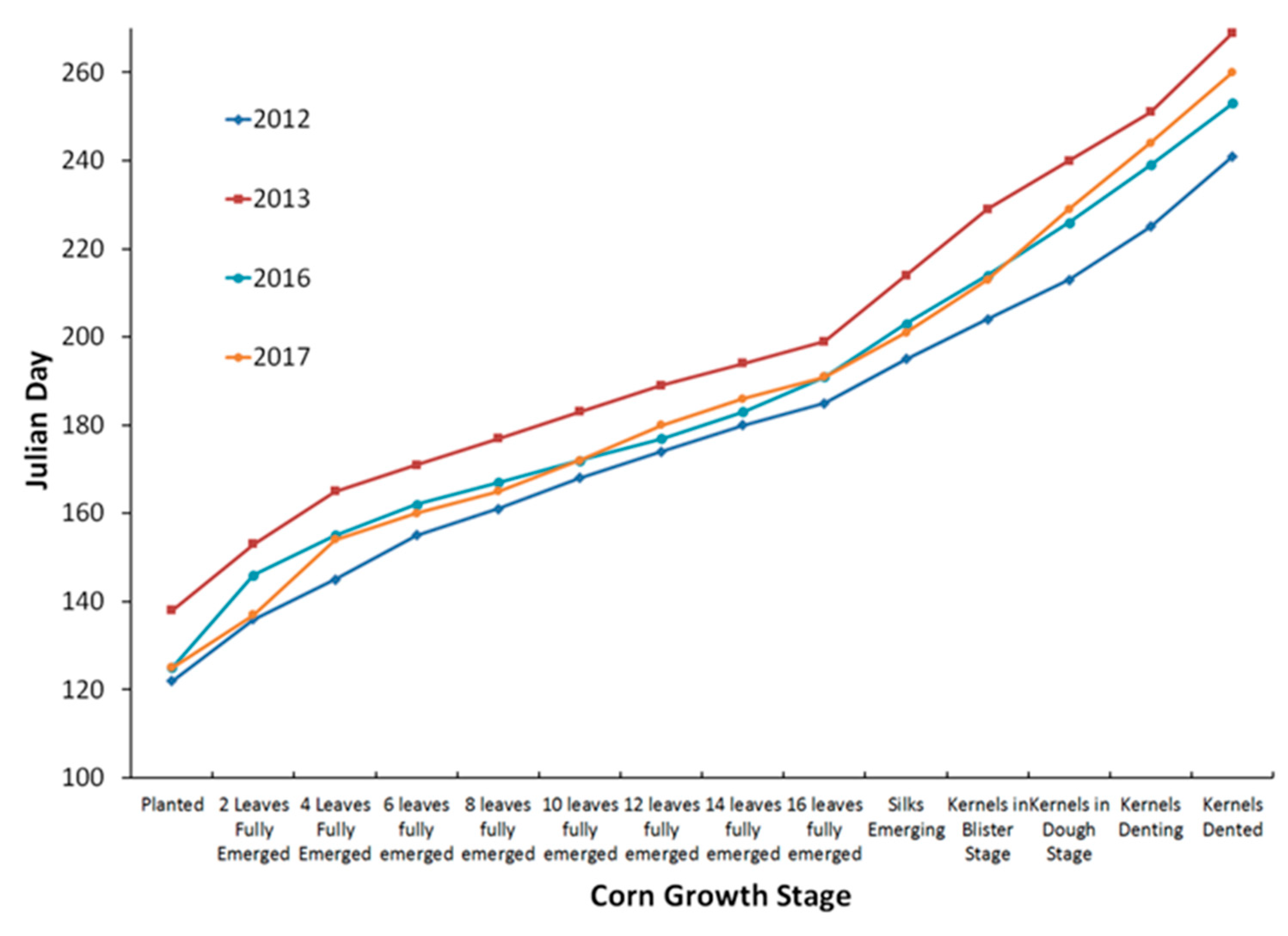
As shown in
Figure 9, the corn growth stages of 2012 (in dark blue) are recorded consistently earlier than 2013 (in red) in the entire growing season.
Figure 9 also shows, in the early growing season (from two Leaves Fully Emerged to eight Leaves Fully Emerged), the corn growth stages in 2017 were earlier than 2016; while in the late growing season (from Kernels Blister to Physiological Maturity), 2017 corn growth stages became later than 2016. Overall, the corn phenologies in 2016 and 2017 are very close as shown in
Figure 4 and
Figure 9. The precise growth stage estimation as shown in
Table 2 and
Figure 9 is critical for further crop growth condition estimation.
To evaluate the results of the estimated corn growth stages, we used NASS reported survey data, as shown in
Table 3, from Iowa Crop Progress and Condition (2012–2017) [
43] in west central Iowa, where Carroll County is located. Those data are the best available reference data. NASS reported only five stages including planting, emergence, silking, dented, and mature at agricultural statistics district (ASD) level. No other more detailed information is available for validation. In
Table 3, the numbers under every date represent the percentages of the corn that reached the growth stages shown on the first column on that date.
As shown in
Table 3, corn emergence was 89% on May 20, 2012, but only 16% on May 19, 2013 (Julian day 139), which suggested that the corn emerged earlier in 2012 than 2013. This is consistent with our estimated results. As shown in
Table 2, the estimated results indicated that the two Leaves Fully Emerged stage was reached on Julian day 136 in 2012, earlier than Julian day 153 in 2013.
Similarly, the estimated results in other years were evaluated in the same way. From
Table 3, we observed that in the early period of corn emergence in 2015, the corn emergence was ahead of 2014 with 62% vs. 39%, which was consistent with the estimated results in
Table 2 (Julian day 138 vs. 144, i.e., 2015 emergence stage is 6 days earlier than 2014). In the main green-up period (from four leaves to 16 leaves fully emerged), the corn grew faster in 2014 than in 2015 as shown in
Table 2. But there were no corresponding data available in NASS report. At the silking stage, the silked percentage in 2014 was higher than that in 2015 as shown in
Table 3 (72% vs. 54% on Julian day 202 and 201 respectively) while
Table 2 shows that crop reached Silks Emerging stage on Julian day 208 in 2014 and 207 in 2015, respectively. However, these two tables reported on the silking stage on the different dates, about six days of difference. Therefore, the comparison result is inconclusive. For 2016 and 2017,
Table 2 and
Table 3 also show that crop in 2017 obviously lags in late growth stages (middle August to September) than in 2016. The estimated results were roughly consistent with NASS reported data in consideration of uncertainties from the estimated results and NASS report as well as the fact that the ASD was much larger than Carroll County.
4.2. Corn Growth Condition Assessment with NDVI and AAT
Table 4 shows early stage crop condition data analysis, which demonstrates how to monitor the weekly corn growth change using NDVI and AAT deviation (ΔNDVI and ΔAAT) proposed in this paper.
Table 4 lists three successive weeks of NDVI and AAT changes quantitatively for four years. Both NDVI and AAT deviations (ΔNDVI and ΔAAT) for each week are listed for 2011, 2012, 2016, and 2017 correspondingly. Usually, the more ΔAAT the corn received, the more ΔNDVI occurred as shown in the column of 2011 in
Table 4 since proper heat conditions can boost corn growth and shows better vegetative condition. However, it is not always the case. The vegetation change also depends on the water supply, fertilization, and growth stage, etc. If corn received a good amount of heat and the NDVI changed little or even decreased, it might signal a stress environment such as drought. This type of abnormal information is very important in crop condition monitoring.
Table 5 shows corn growth assessment results based on the same growth stage (SGS) (usually different Julian day) and the same Julian day (SJD) (maybe at a different growth stage) in 2012 and 2017. Years 2011 and 2016 data are used for comparison references. The average of multi-year historical data was not used as the baseline for comparison since there were no direct ground truth data available for validation analysis. Three growth stages including eight leaves fully emerged (date1 in
Table 5), 14 leaves fully emerged (date2), and silking (date3) were sampled for comparison. On each date, corn NDVI and NDVI departure (ΔNDVI) from the reference year are listed together.
For the first comparison, corn in 2012 reached to the stage of eight leaves fully emerged on Julian day 161 when the NDVI was 0.611. When it reached to the same stage on Julian day 172 in 2011 (as shown in column 2011-SGS), the NDVI value was at 0.617. The NDVI deviation from 2011 reference was –0.006, which meant that at the stage of eight leaves fully emerged, the corn growth condition was worse than that in 2011. However, as shown in
Table 5, column 2011-SJD, the NDVI assessed based on the same Julian day (161) in 2011, was significantly lower at 0.497 with a NDVI deviation of +0.114, which meant the growth condition was better than that in 2011. Similarly, the NDVI value (0.827) at the stage of 14 leaves fully emerged in 2012 was smaller than NDVI value (0.847) at the SGS in 2011, but much bigger than the NDVI value (0.736) at the SJD in 2011.
As the second comparison, it was observed from
Table 5 that the 2017 NDVI values at the sampled growth stages were all lower than those both at the same Julian day and at the same growth stages in 2016 though the NDVI differences between 2017 and 2016 at the different growth stages varied. It was observed that the dates of the sampled three corn growth stages in 2017 were very close to those in 2016, only 2–3 days apart. This may explain why the crop NDVI comparison results based on SGS and SJD are consistent though their NDVI departure amplitudes were different.
To determine which comparison result is closer to reality, the NASS published survey report data were used as ground reference for validation. The NASS reported data provide five categories of crop growth conditions as shown in
Table 6.
Table 6 illustrates the crop conditions reported by NASS on three sampled corn crop growth stages of 2012 and 2017, and their corresponding references (2011 and 2016), which are approximately aligned at the same growth stages. The first two rows in
Table 6 list the NASS reported corn growth conditions on Julian day 162 in 2012 and on Julian day 170 in 2011, which are the closest to the date1 in
Table 5 (the data on the same day are unavailable).
As shown in
Table 6, the percentages of good and excellent conditions combined are 67% and 84% respectively in 2012 and 2011, which suggest that corn growth condition in 2012 is worse than that in 2011. Similarly, the assessed results on date2 and date3 (as shown in
Table 5) in 2012 are also consistent with the NASS reported results corresponding to stages of 14 leaves fully emerged and silking in
Table 6. From
Table 6, the percentages of good and excellent conditions combined are 62% and 82% for 14 leaves fully emerged on date2 and 36% and 80% for silking on date3 respectively in 2012 and 2011. Both
Table 5 and
Table 6 indicate that corn vegetation conditions in 2012 are worse than that in 2011.
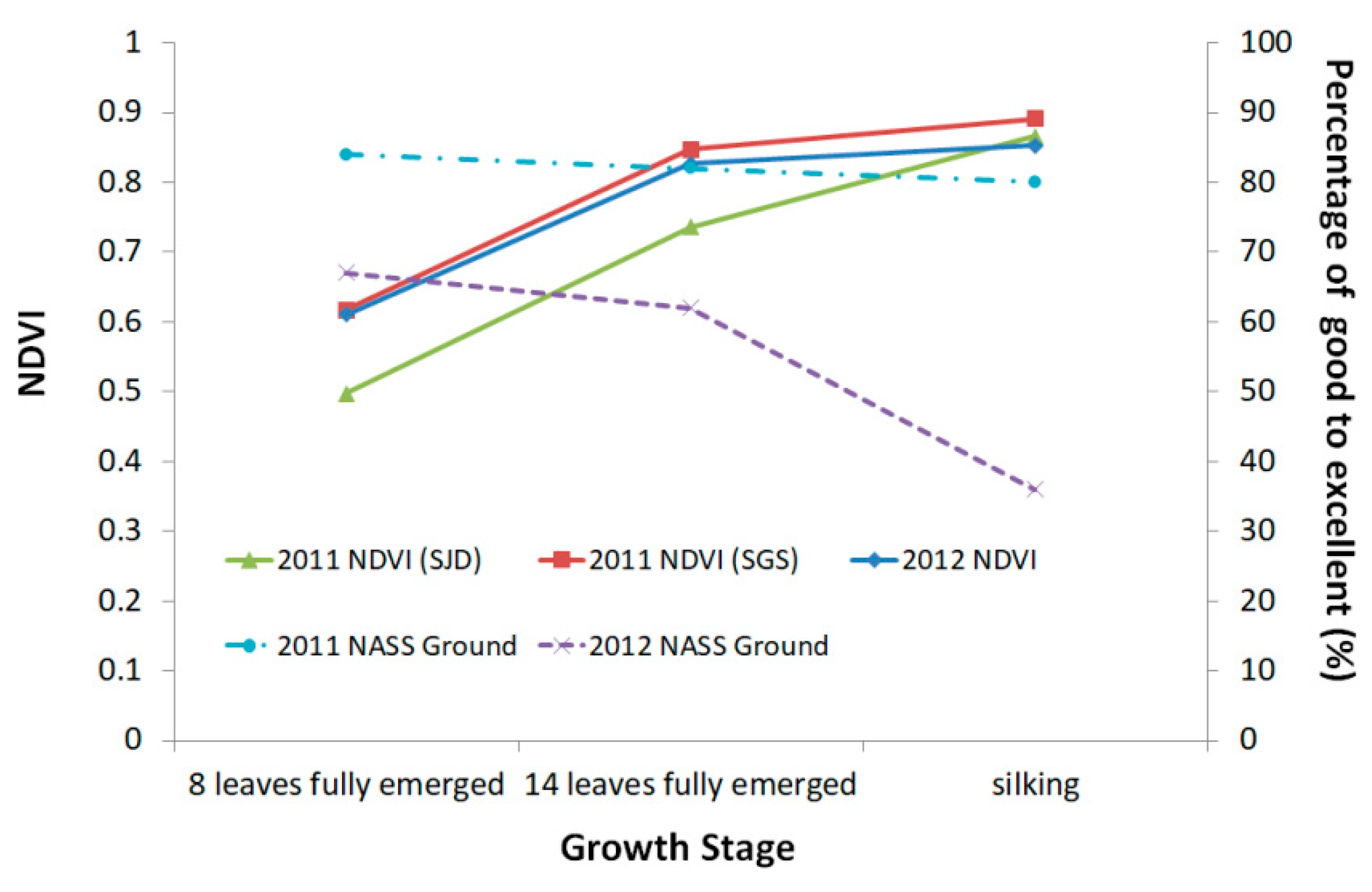
These comparisons are also clearly illustrated in
Figure 10 for better understanding. As shown in
Figure 10, the differences between 2012 and 2011 NASS reported good and excellent conditions (purple dashed line and blue dash dot lines) (17%, 20%, and 44% respectively as calculated from
Table 6) for three selected growth stages are increasing monotonically as the crop growth stage progresses. The purple dashed line is entirely under the blue dash dot lines. Meanwhile, the 2012 NDVI (blue solid line) is below in 2011 NDVI at SGS (red solid line). These results indicate that assessment results aligned at SGS are consistent with the NASS reported crop condition results. Both of them suggest the crop conditions at the three sampled stages in 2012 are worse than those in 2011, and become worse and worse along the growth stage progress. The comparison result between 2012 NDVI (blue solid line) and 2011 SJD NDVI (green solid line) is not consistent with yearly comparison result of NASS reported crop condition data. Similarly, 2016 and 2017 crop condition comparison could be presented in the same manner, which is omitted here to avoid tedious description.
The corn growth conditions on the sampled growth stages in 2017, as shown in
Table 5 and
Table 6, both are worse than that in 2016 though the conditions of both years are very close, especially at the stage of 14 leaves fully emerged (date2). As shown in
Table 6, the combined good and excellent conditions pairs for 2017, 2016 are (77%, 80%), (78%, 79%), and (68%, 82%) for three sampled growth stages respectively. Overall, the proposed corn crop growth condition assessment results are consistent with the NASS reported results when the assessment are based on the same growth stage.
As mentioned above, the assessment based on the same Julian day was not consistent with the results yielded from the same growth stages. Therefore, the assessment results based on the same Julian day are not consistent with the results reported by the NASS weekly Crop Progress and Condition Report. This indicates that the crop growth condition assessment based on the same Julian (calendar) day may be less robust than that based on the same growth stage.
5. Discussion
The experimental results presented in the previous sections indicate that the AAT-based method can successfully extract more detailed corn growth stages than that based on remotely sensed NDVI data though the NDVI can provide more information on corn crop vegetative condition. For every day in a given corn growing season, a corresponding date can be found in the reference year at the same growth stage with the given ΔAAT after corn planting. This is the base on which crop growth conditions can be assessed based on growth stages. Moreover, the difference between the dates of the given year and the reference year indicates the corn crop of the given year developing earlier or later. The AAT-based corn growth stage estimates may further facilitate the corn growth condition assessment. For example, corn at any growth stage can be further classified into different growth condition categories such as very poor, poor, fair, good, and excellent based on a comparison with the baseline conditions. This categorization needs multi-year, large scale ground truth data collection for validation and calibration. With sufficient ground truth data, NDVI thresholds for each corn crop condition category can be found. However, the quantitative assessment of the crop growth conditions is readily available by comparing NDVIs of different years.
The daily AAT monitoring should begin far before the corn growing season starts in order to determine the suitable planting time. The current year AAT curve can be used to monitor abnormal temperature changes in real time and to assess their further impact on crop growth or on crop yield.
The temperatures beyond the lower or upper threshold temperature, 50 or 86 °F respectively, was neglected in this paper. They do not affect the AAT calculation and the growth stage estimation. However, these temperatures can be used for monitoring disasters associated with temperature and for further assessment of corn growth condition under environmental stress. The gridding product Daymet data is used for AAT calculation in this study. The Daymet is not a real-time data product and is not appropriate for real-world operational use. However, AAT data can be derived from the interpolated ground station data, or even from remotely sensed surface temperature data, which are near real-time and suitable for operational use. Using the remotely sensed surface temperature data for AAT estimation will be further investigated in our future work.
Raw daily NDVI time series were reconstructed in this study through correction and smoothing to eliminate clouds, noise, and other distortion. Different smoothing methods may produce NDVI time series with different accuracies. The impact of different smoothing methods on growth condition assessment accuracy needs to be further assessed in the future.
The NDVI combined with AAT can predict the future crop growth stage and condition if the future temperature can be forecasted. One of the big problems in this study is that there are not enough detailed county level or sub-county level ground truth data available for validation. NASS reported crop condition and progress statistics at district or state level only (a few states with district level report). Therefore, it is difficult to assess the accuracy at the pixel level (250 m resolution MODIS data). If sufficient pixel level ground truth data were available, assessment at pixel level can be performed to capture more detailed spatial variations. In addition, larger scale assessment such as ASD or state level should also be considered to match with NASS’s reported survey for better validation and possible calibration. The crop condition validation assessment was performed on two individual years since no five-year averaged reference data were readily available for validation from NASS reports.
The methodology presented here is complicated. The motivation for this research is to develop an effective methodology that can produce useful information to help corn producers manage their production and to help other users for their decision making support. In future, an operational online GIS application can be developed to automatically produce crop condition information and freely disseminate the information over the web so that producers and other users have equal access to the information.
Fusion of multisensory data, such as MODIS, Landsat 8, and Sentinel-2 data should be investigated to improve spatial and temporal resolution and consequently to further improve the crop growth condition assessment accuracy in future studies.
6. Conclusions
The study aimed to develop a reliable method for large scale operational crop growth condition monitoring, which enabled us to derive county or sub-county crop specific growth condition assessment with no crop mismatch. The reliability of remote-sensing based crop condition assessment is challenging due to the misalignment of crop growth stages when NDVIs of different years are compared. The AAT-aligned approach proposed in this paper provides a solution for crop condition assessment based on aligned crop growth stages. The crop growth stages of different years can be easily matched based on the AAT after planting. This study successfully assessed crop growth conditions at county level using NDVI time series based on the aligned crop growth stages of two different years via AATs.
As AAT is mainly used in the process to measure the heat that boosts the crop growth, the proposed method can also be called the heat-aligned method, which can be understood more easily by those who do not know the AAT in advance. Moreover, AAT can not only help align the crop growth stages between years, but also provide other important information associated with crop growing environment, which maybe contribute to more effective crop condition assessment or crop yield estimation, even temperature-associated disaster monitoring or crop lost predicting.
This study demonstrates the cloudy and noisy pixels can be successfully filtered, and NDVI time series can be effectively reconstructed from the daily 250 m resolution MODIS surface reflectance data by using both Best Index Slope Extraction (BISE) and Savitzky–Golay.
The crop condition assessment results based on the same crop growth stages and the same calendar dates were compared and evaluated with the published NASS report reference data. The study indicates that the results of crop growth condition assessment with aligned growth stages are consistent with the NASS reported results but not consistent with the results of assessment with the same Julian days. This finding indicates that assessing corn growth conditions based on the growth stages is more reliable than the results based on the same Julian days. Overall, the proposed method can effectively measure crop growth condition changes with the information of biomass and heat supply changes from NDVI and AAT data.
Author Contributions
Conceptualization, Z.Y., Y.Q., L.D.; Methodology, Y.Q. and Z.Y.; Software, M.S.R., L.X. and Z.T.; Validation, Y.Q. and Z.Y., F.G.; Formal Analysis, Y.Q., Z.Y.; Investigation, Y.Q. and Z.Y.; Resources, L.D., Z.Y. and E.G.Y.; Data Curation, Y.Q.; Writing—Original Draft Preparation, Y.Q.; Writing—Review and Editing, Y.Q. and Z.Y., F.G., X.Z.; Visualization, Y.Q.; Supervision, Z.Y., L.D.; Project Administration, Z.Y., L.D.
Funding
This research was supported by China Scholarship Council.
Acknowledgments
The study was accomplished in the Center for Spatial Information Science and Systems, George Mason University, VA, United States of America.
Conflicts of Interest
The authors declare no conflict of interest.
Disclaimer
The findings and conclusions in this publication are those of the authors and should not be construed to represent any official USDA or U.S. Government determination or policy.
References
- Tucker, C.J.; Elgin, J.H., Jr.; McMurtrey, J.E., III; Fan, C.J. Monitoring corn and soybean crop development with hand-held radiometer spectral data. Remote Sens. Environ. 1979, 8, 237–248. [Google Scholar] [CrossRef]
- Gardner, B.R.; Blad, B.L.; Thompson, D.R.; Henderson, K.E. Evaluation and interpretation of Thematic Mapper ratios in equations for estimating corn growth parameters. Remote Sens. Environ. 1985, 18, 225–234. [Google Scholar] [CrossRef]
- Hatfield, J.L.; Kanemasu, E.T.; Asrar, G.; Jackson, R.D.; Pinter, P.J., Jr.; Reginato, R.J.; Idso, S.B. Leal-area estimates from spectral measurements over various planting dates of wheat. Int. J. Remote Sens. 1985, 6, 167–175. [Google Scholar] [CrossRef]
- Wiegand, C.L.; Richardson, A.J.; Escobar, D.E.; Gerbermann, A.H. Vegetation indices in crop assessments. Remote Sens. Environ. 1991, 35, 105–119. [Google Scholar] [CrossRef]
- Gallo, K.P.; Flesch, T.K. Large-area crop monitoring with the NOAA AVHRR: Estimating the silking stage of corn development. Remote Sens. Environ. 1989, 27, 73–80. [Google Scholar] [CrossRef]
- Gupta, R.K. NOAA/AVHRR vegetation indices and agriculture-meteorology processes. Adv. Space Res. 1992, 12, 87–90. [Google Scholar] [CrossRef]
- Hmimina, G.; Dufrêne, E.; Pontailler, J.-Y.; Delpierre, N.; Soudani, K. Evaluation of the potential of MODIS satellite data to predict vegetation phenology in different biomes: An investigation using ground-based NDVI measurements. Remote Sens. Environ. 2013, 132, 145–158. [Google Scholar] [CrossRef]
- Nagy, A.; Fehér, J.; Tamás, J. Wheat and maize yield forecasting for the Tisza river catchment using MODIS NDVI time series and reported crop statistics. Comput. Electron. Agric. 2018, 151, 41–49. [Google Scholar] [CrossRef]
- Reichert, G.C.; Caissy, D. A Reliable Crop Condition Assessment Program (CCAP) Incorporating NOAA AVHRR Data, A Geographical Information System and the Internet. 2002. Available online: http://proceedings.esri.com/library/userconf/proc02/pap0111/po111.htm (accessed on 6 June 2014).
- Rebeca, G.; Reyna-Trujillo, T.; Soria-Ruiz, J.; Gómez-Rodríguez, G. Analysis of NOAA-AVHRR-NDVI images for crops monitoring. Int. J. Remote Sens. 2004, 25, 1615–1627. [Google Scholar]
- Fensholt, R.; Rasmussen, K.; Nielsen, T.T.; Mbow, C. Evaluation of earth observation based long term vegetation trends—Intercomparing NDVI time series trend analysis consistency of Sahel from AVHRR GIMMS, Terra MODIS and SPOT VGT data. Remote Sens. Environ. 2009, 113, 1886–1898. [Google Scholar] [CrossRef]
- Yang, Z.W.; Di, L.P.; Yu, G.P.; Chen, Z.Q. Vegetation Condition Indices for Crop Vegetation Condition Monitoring. In Proceedings of the 2001 IEEE International Geoscience and Remote Sensing Symposium (IGARSS), Vancouver, BC, Canada, 24–29 July 2011; pp. 3534–3537. [Google Scholar]
- Miao, Z.; Wu, B.; Yu, M.; Zou, W.; Zheng, Y. Crop Condition Assessment with Adjusted NDVI Using the Uncropped Arable Land Ratio. remote sensing. Remote Sens. 2014, 6, 5774–5794. [Google Scholar] [CrossRef]
- Rangoonwala, A.; Ahmed, S.; Nasir, A.; Raouf, A.; Shahab, H. Quasi-operational use of NOAA/AVHRR vegetation index to monitor vegetal cover and crop growth. Adv. Space Res. 1993, 13, 265–268. [Google Scholar] [CrossRef]
- Esquerdo, J.C.D.M.; Zullo, J.J.; Antunes, J.F.G. Use of NDVI/AVHRR time-series profiles for soybean crop monitoring in Brazil. Int. J. Remote Sens. 2011, 32, 3711–3727. [Google Scholar] [CrossRef]
- Meng, J.H.; Wu, B.F. Study on the crop condition monitoring methods with remote sensing. Remote Sens. Spat. Inf. Sci. 2008, 37, 945–950. [Google Scholar]
- Qian, Y.; Hou, Y.; Yan, H.; Mao, L.; Wu, M.; He, Y. Global crop growth condition monitoring and yield trend prediction with remote sensing. Trans. Chin. Soc. Agric. Eng. (Trans. CSAE) 2012, 28, 166–171. [Google Scholar]
- Pei, Z.; Yang, B. Analysis of multi-temporal and multi-spatial character of NDVI and crop condition models development. Trans. Chin. Soc. Agric. Eng. (Trans. CSAE) 2000, 16, 20–22. [Google Scholar]
- Crop Progress and Condition, United States of Agriculture, National Agricultural Statistics Service. Available online: https://www.nass.usda.gov/Charts_and_Maps/Crop_Progress_&_Condition/index.php (accessed on 30 June 2019).
- Reed, B.C.; Brown, J.F.; Vander Zee, D.; Loveland, T.R.; Merchant, J.W.; Ohlen, D.O. Measuring phenological variability from satellite imagery. J. Veg. Sci. 1994, 5, 703–714. [Google Scholar] [CrossRef]
- Jonsson, P.; Eklundh, L. TIMESAT—A program for analysing time-series of satellite sensor data. Comput. Geosci. 2004, 30, 833–845. [Google Scholar] [CrossRef]
- Zhang, X.Y. Land Surface Phenology: Climate Data Record and Real-Time Monitoring. In Comprehensive Remote Sensing: Terrestrial ecosystems, 1st ed.; Liang, S., Ed.; Elsevier: New York, NY, USA, 2017; pp. 35–52. [Google Scholar]
- Gao, F.; Martha, C.; Anderson, A.; Zhang, X.; Yang, Z.; Joseph, G.; Alfieri, W.; Kustas, P.; Mueller, R.; David, M.; et al. Toward mapping crop progress at field scales through fusion of Landsat and MODIS imagery. Remote Sens. Environ. 2017, 188, 9–25. [Google Scholar] [CrossRef] [Green Version]
- Accumulated Temperature, Meteorology Glossary, American Meteorological Society. Available online: http://glossary.ametsoc.org/wiki/Accumulated_temperature (accessed on 25 April 2012).
- Mederski, H.J.; Miller, M.E.; Weaver, C.R. Accumulated heat units for classifying corn hybrids maturity. Agron. J. 1973, 65, 743–747. [Google Scholar] [CrossRef]
- Gilmore, E.C.; Rogers, J.S. Heat units as a method of measuring maturity in corn. Agron. J. 1958, 50, 611–615. [Google Scholar] [CrossRef]
- Neild, R.E.; Newman, J.E. Growing Season Characteristics and Requirements in the Corn Belt; NCH-40; Cooperative Extension Service, Purdue University: West Lafayette, IN, USA, 1990. [Google Scholar]
- Boryan, C.; Yang, Z.; Mueller, R.; Craig, M. Monitoring US agriculture: The US Department of Agriculture, National Agricultural Statistics Service, Cropland Data Layer Program. Geocarto Int. 2011, 26, 341–358. [Google Scholar] [CrossRef]
- Han, W.; Yang, Z.; Di, L.; Mueller, R. CropScape: A Web service based application for exploring and disseminating US conterminous geospatial cropland data products for decision support. Comput. Electron. Agric. 2012, 84, 111–123. [Google Scholar] [CrossRef]
- Thornton, P.E.; Thornton, M.M.; Mayer, B.W.; Wei, Y.; Devarakonda, R.; Vose, R.S.; Cook, R.B. Daymet: Daily Surface Weather Data on a 1-km Grid for North America, Version 3; ORNL DAAC: Oak Ridge, TN, USA, 2018. [CrossRef]
- Michishita, R.; Jin, Z.; Chen, J.; Xu, B. Empirical comparison of noise reduction techniques for NDVI time-series based on a new measure. ISPRS J. Photogramm. Remote Sens. 2014, 91, 17–28. [Google Scholar] [CrossRef]
- Rahman, M.S.; Di, L.; Shrestha, R.; Eugene, G.Y.; Lin, L.; Kang, L.; Deng, M. Comparison of Selected Noise Reduction Techniques for MODIS Daily NDVI: An Empirical Analysis on Corn and Soybean. In Proceedings of the Fifth International Conference on Agro-Geoinformatics, Tianjin, China, 18–20 July 2016. [Google Scholar]
- Kandel, H.; Akyuz, A. Growing Degree Day Model for North Dakota Soybean. 2012. Available online: https://www.ag.ndsu.edu/cpr/plant-science/growing-degree-day-model-for-north-dakota-soybean-6-28-12 (accessed on 28 June 2012).
- Abendroth, L.J.; Elmore, R.W.; Boyer, M.J.; Marlay, S.R. Corn Growth and Development; PMR 1009; Iowa State University Extension: Ames, IA, USA, 2011. Available online: https://www.nass.usda.gov/Statistics_by_State/Iowa/Publications/Crop_Progress_&_Condition/index.php (accessed on 12 October 2019).
- Elmore, R.; Mueller, N. Growing Degree Units and Corn Emergence. 2015. Available online: https://cropwatch.unl.edu/growing-degree-units-and-corn-emergence (accessed on 12 May 2015).
- Anandhia, A. Growing degree days—Ecosystem indicator for changing diurnal temperatures and their impact on corn growth stages in Kansas. Ecol. Indic. 2016, 61, 149–158. [Google Scholar] [CrossRef]
- Poonia, S.; Singh, G.; Malik, D.S. Influence of sowing dates on the growing degree days and phenology of winter maize. Agric. For. Meteorol. 1986, 38, 47–57. [Google Scholar]
- Oluwaranti, A.; Fakorede, M.A.B.; Adeboye, F.A. Maturity Groups and Penology of Maize in a Rainforest Location. Int. J. Agric. Innov. Res. 2015, 4. Available online: http://www.ijair.org/administrator/components/com_jresearch/files/publications/IJAIR_1486_Final.pdf (accessed on 30 June 2019).
- Wang, J.Y. A critique of the heat unit approach to plant response studies. Ecology 1960, 41, 785–790. [Google Scholar] [CrossRef]
- Duncan, S.; Fjell, D.; Vanderlip, R. Handbook of Corn Production; Kansas State University Agricultural Experiment Station and Cooperative Extension Service Publication: Manhattan, KS, USA, 2010; p. 43. [Google Scholar]
- Shaw, R.H. Growing-Degree Units for Corn in the North Central Region; No. 581; Article 1; Research Bulletin for Iowa Agriculture and Home Economics Experiment Station: Ames, IA, USA, 1975; Volume 36, Available online: http://lib.dr.iastate.edu/researchbulletin/vol36/iss581/1 (accessed on 12 October 2019).
- McMaster, G.S.; Wilhelm, W.W. Growing degree-days: One equation, two interpretations. Agric. For. Meteorol. 1997, 87, 291–300. [Google Scholar] [CrossRef]
- Iowa Crop Progress & Condition (2012–2017), USDA, National Agricultural Statistics Service. Available online: https://www.nass.usda.gov/Statistics_by_State/Iowa/Publications/Crop_Progress_&_Condition/index.php (accessed on 30 June 2019).
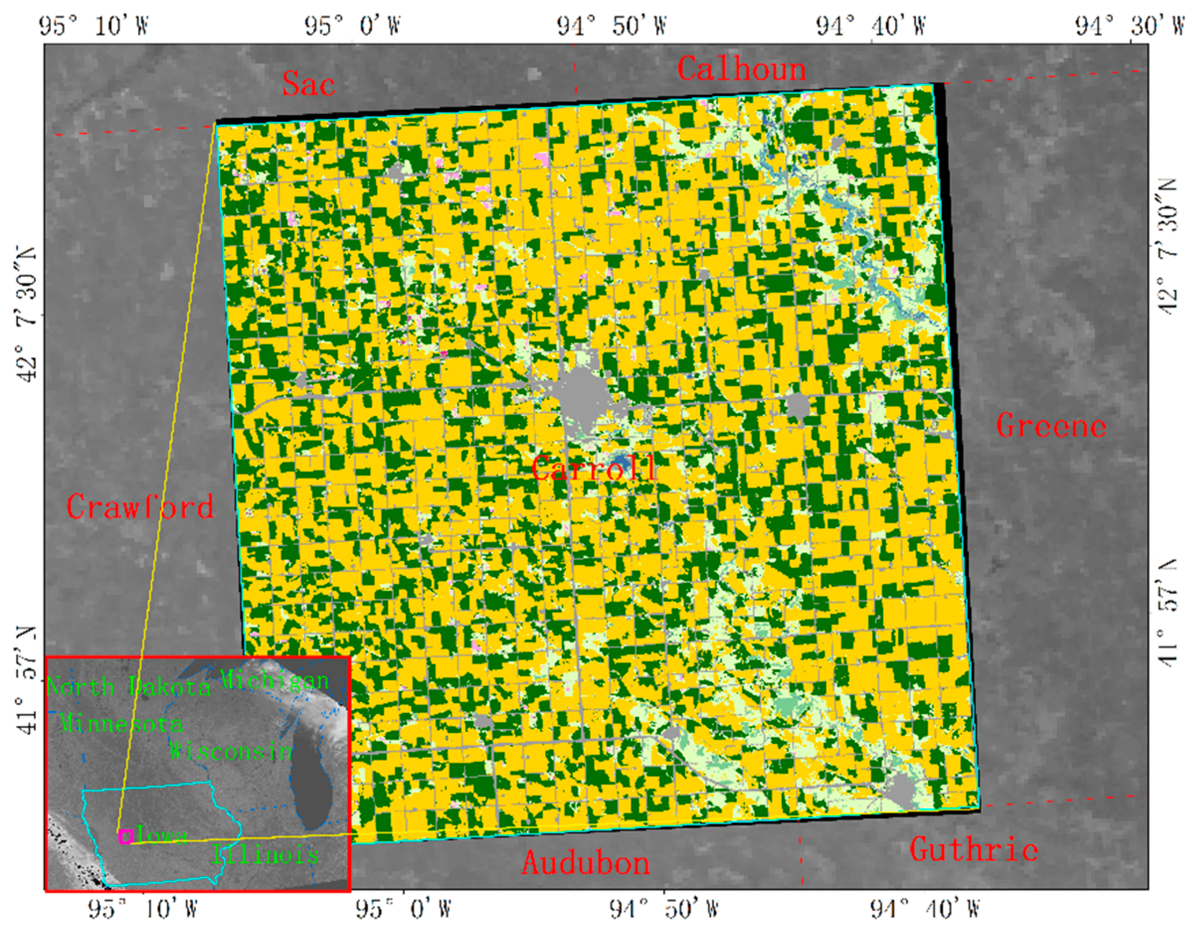
Figure 1.
The study area (Carroll County) in the State of Iowa, U.S. The background grey map is daily MODIS NDVI image. The blue boundary in the small overview map overlaid at the lower left corner illustrates the State of Iowa. The color map overlaid in the middle is the NASS Cropland Data Layer (CDL) map of Carroll County. The dark green, yellow, and grey represent soybeans, corn, and development/open space categories. The light green and pink represent grass land and alfalfa.
Figure 2.
Flowchart of the corn growth condition assessment methodology based on heat-aligned crop growth stages. The left part shows the procedures for producing noise-filtered NDVI time series data; the right part illustrates the procedures for computing active accumulated temperature (AAT), estimating corn growth stage and assessing crop growth conditions based on aligned crop growth stages.
Figure 3.
The original (in blue) and smoothed (in red) NDVI time series of a pure corn pixel. The extremely lower NDVI values (in blue) were removed and reconstructed by filtering and smoothing process.
Figure 3.
The original (in blue) and smoothed (in red) NDVI time series of a pure corn pixel. The extremely lower NDVI values (in blue) were removed and reconstructed by filtering and smoothing process.
Figure 4.
The corn phenologies in Carroll County from 2007 to 2017 and the NDVI baseline (dashed line). The corn phenology of the year 2012 (orange line) is abnormal and excluded from NDVI baseline calculation. The 2017 NDVI is the study target and its NDVI is not in the baseline calculation.
Figure 4.
The corn phenologies in Carroll County from 2007 to 2017 and the NDVI baseline (dashed line). The corn phenology of the year 2012 (orange line) is abnormal and excluded from NDVI baseline calculation. The 2017 NDVI is the study target and its NDVI is not in the baseline calculation.
Figure 5.
(a) Left is the raw NDVI image and its histogram, and (a) Right is the smoothed NDVI image and its histogram. The smoothed and reconstructed NDVI image illustrates field and land cover patterns and its histogram is concentrated around 0.9, which is consistent with peak vegetation period on August 3, 2017. (b) Illustrates the processed NDVI means of 2007 and 2017 in the upper part, and standard deviations of the NDVIs of 2007 and 2017 in the lower part.
Figure 6.
The AAT curves cover the corn growing season in Carroll County from year 2007 to 2017 and the AAT baseline (dashed line). The abnormal year 2012 is excluded in the baseline calculation.
Figure 6.
The AAT curves cover the corn growing season in Carroll County from year 2007 to 2017 and the AAT baseline (dashed line). The abnormal year 2012 is excluded in the baseline calculation.
Figure 7.
Corn NDVI curve (corn phenology) and AAT curve covering the growing season of 2012 (a given study year) are compared with the baseline based on the same Julian calendar day. The green solid and black dashed lines are 2012 NDVI curve and NDVI baseline, respectively. The pink solid and red dashed lines are 2012 AAT curve and AAT baseline. Compared with the NDVI baseline, the 2012 corn phenology is significantly earlier than baseline (the entire NDVI curve appears left of the baseline). The 2012 AAT curve is above the ATT baseline, which means 2012 crop reaches the same growth stages earlier.
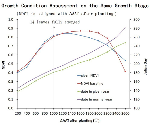
Figure 8.
The NDVIs and the needed Julian dates corresponding to the ΔAATs of the given year and the normal reference year. The baseline (normal year) and the given study year NDVI curves (corn phenology) are in red and blue respectively. The purple and green curves represent the dates that crops reach the same growth stages (or the same ΔAAT) in the normal year and the given study year, respectively. For a given ΔAAT (or growth stage), comparing two NDVI values gives the indication of the crop growth condition while comparing Julian days provides information of timing of reaching at the given crop growth stage.
Figure 9.
Estimated corn growth stages comparison in 2012, 2013, 2016, and 2017.
Figure 9.
Estimated corn growth stages comparison in 2012, 2013, 2016, and 2017.
Figure 10.
The 2012 NDVIs at SGS and 2011 NDVIs at SGS and SJD and corresponding NASS reported data for validation. The x-axis represents 2012 growth stage (with Julian date). The 2011 NDVIs at SGS and SJD are in red and green solid lines respectively. They are aligned with 2012 growth stages and Julian day respectively. The 2012 NDVI at SGS is in blue solid line. The 2012 NASS reported percentage of crop in good and excellent categories (in purple dashed line) is lower than the corresponding 2011 NASS reported data (in light blue dash dot line). Obviously, the results based on SJD NDVI (green solid line) are not consistent with the NASS reported crop condition data.
Table 1.
Corn growth stages and growing degree units.
Table 1.
Corn growth stages and growing degree units.
| Phase | Development Stage | ΔAAT (°F) |
|---|
| Vegetative | Planted | 0 |
| Two Leaves Fully Emerged | 200 |
| Four Leaves Fully Emerged | 345 |
| Six leaves fully emerged (Growing Point above Soil) | 475 |
| Eight leaves fully emerged (Tassel Beginning to Develop) | 610 |
| 10 leaves fully emerged (Rapid Growth Phase begins) | 740 |
| Reproductive | 12 leaves fully emerged (Ear Formation) | 870 |
| 14 leaves fully emerged (Silks Developing on Ear) | 1000 |
| 16 leaves fully emerged (Tip of Tassel Emerging) | 1135 |
| Silks Emerging/Pollen Shedding (Plant at full height) | 1400 |
| Maturation | Kernels in Blister Stage | 1660 |
| Kernels in Dough Stage | 1925 |
| Kernels Denting | 2190 |
| Kernels Dented | 2450 |
| Physiological Maturity | 2700 |
Table 2.
ΔAAT-aligned corn growth stages identified in Julian days in Carroll County from year 2012 to 2017.
Table 2.
ΔAAT-aligned corn growth stages identified in Julian days in Carroll County from year 2012 to 2017.
| | 2012 | 2013 | 2014 | 2015 | 2016 | 2017 | 5y-avg 2 |
|---|
| Planted | 122 | 138 | 123 | 118 | 125 | 125 | 123 |
| Two Leaves Fully Emerged | 136 | 153 | 144 | 138 | 146 | 137 | 142 |
| Four Leaves Fully Emerged | 145 | 165 | 151 | 154 | 155 | 154 | 152 |
| Six leaves fully emerged | 155 | 171 | 158 | 161 | 162 | 160 | 160 |
| Eight leaves fully emerged | 161 | 177 | 167 | 168 | 167 | 165 | 167 |
| 10 leaves fully emerged | 168 | 183 | 173 | 175 | 172 | 172 | 172 |
| 12 leaves fully emerged | 174 | 189 | 179 | 181 | 177 | 180 | 178 |
| 14 leaves fully emerged | 180 | 194 | 187 | 190 | 183 | 186 | 185 |
| 16 leaves fully emerged | 185 | 199 | 194 | 196 | 191 | 191 | 191 |
| Silks Emerging | 195 | 214 | 208 | 207 | 203 | 201 | 203 |
| Kernels in Blister Stage | 204 | 229 | 223 | 219 | 214 | 213 | 215 |
| Kernels in Dough Stage | 213 | 240 | 236 | 233 | 226 | 229 | 228 |
| Kernels Denting | 225 | 251 | 251 | 248 | 239 | 244 | 242 |
| Kernels Dented | 241 | 269 | 282 | 266 | 253 | 260 | 257 |
| Physiological Maturity | 252 | — 1 | — | 297 | 268 | 276 | 284 |
Table 3.
Corn growth monitoring results in the west central district of Iowa released by NASS in different years from 2011 to 2017. In the “Date” rows, the numbers in the parentheses are Julian date corresponding to the calendar (Gregorian) date.
Table 3.
Corn growth monitoring results in the west central district of Iowa released by NASS in different years from 2011 to 2017. In the “Date” rows, the numbers in the parentheses are Julian date corresponding to the calendar (Gregorian) date.
| Year | 2012 | 2013 | 2014 | 2015 | 2016 | 2017 |
|---|
| Date | 05/20(141) | 05/19(139) | 05/18(139) | 05/17(137) | 05/22(143) | 05/21(141) |
| Planted (%) | 99 | 78 | 94 | 92 | 95 | 89 |
| Emerged (%) | 89 | 16 | 39 | 62 | 73 | 64 |
| Date | 07/15(197) | 07/21(202) | 07/20(201) | 07/19(200) | 07/17(199) | 07/16(197) |
| Tasseled (%) | 94 | 43 | — | — | — | — |
| Silked (%) | 83 | 21 | 72 | 54 | 71 | 45 |
| Date | 09/16(260) | 09/22(265) | 09/21(264) | 09/20(263) | 09/18(262) | 09/17(260) |
| Dented (%) | — | 93 | 97 | 98 | 94 | 85 |
| Matured (%) | 84 | 36 | 55 | 42 | 41 | 27 |
Table 4.
Weekly changes of corn NDVIs and AATs in Carroll County at corn emergence period of different years. In the week of May 13th to May 20th (05/13–05/20) of 2011, ΔNDVI and ΔAAT are 0.014 and 34 °F, respectively, which means that the corn NDVI has changed 0.014 after it receives 34 °F ΔAAT during the week.
| Date | Changes | 2011 | 2012 | 2016 | 2017 |
|---|
| 05/13–05/20 | ΔNDVI | 0.014 | 0.021 | 0.012 | 0.006 |
| ΔAAT (°F) | 34 | 121 | 23 | 88 |
| 05/20–05/27 | ΔNDVI | 0.023 | 0.040 | 0.017 | 0.011 |
| ΔAAT (°F) | 72 | 106 | 106 | 50 |
| 05/27–06/03 | ΔNDVI | 0.041 | 0.068 | 0.038 | 0.030 |
| ΔAAT (°F) | 135 | 79 | 121 | 113 |
Table 5.
Comparisons of 2012 and 2017 corn NDVI changes with their previous years of values based on the same growth stages and the same Julian days in Carroll County. The columns 2011-SGS and 2011-SJD, and 2016-SGS and 2016-SJD illustrate 2011 and 2016 NDVI values based on the same growth stages (SGS) and the same Julian days (SJD), and 2012 and 2017 NDVIs’ deviations from 2011 and 2016 correspondingly. Date1, 2, 3 are all in Julian days.
| Growth Stage | Date | 2012 | 2011-SGS | 2011-SJD | 2017 | 2016-SGS | 2016-SJD |
|---|
| Eight leaves fully emerged | Date1 | 161 | 172 | 161 | 165 | 167 | 165 |
| NDVI | 0.611 | 0.617 | 0.497 | 0.578 | 0.647 | 0.615 |
| ΔNDVI | N/A | –0.006 | 0.114 | N/A | –0.069 | –0.037 |
| 14 leaves fully emerged | Date2 | 180 | 191 | 180 | 186 | 183 | 186 |
| NDVI | 0.827 | 0.847 | 0.736 | 0.823 | 0.824 | 0.840 |
| ΔNDVI | N/A | –0.020 | 0.091 | N/A | –0.001 | –0.017 |
| Silking | Date3 | 195 | 206 | 195 | 201 | 203 | 201 |
| NDVI | 0.853 | 0.891 | 0.866 | 0.882 | 0.887 | 0.884 |
| ΔNDVI | N/A | –0.038 | –0.013 | N/A | –0.005 | –0.002 |
Table 6.
NASS reported corn crop condition (dates shown are matching exactly or to the closest dates in
Table 5). All crop conditions are assessed in percentage (%) of the crop felled into the categories.
Table 6.
NASS reported corn crop condition (dates shown are matching exactly or to the closest dates in
Table 5). All crop conditions are assessed in percentage (%) of the crop felled into the categories.
| Growth Stage | Date | Very Poor (%) | Poor (%) | Fair (%) | Good (%) | Excellent (%) |
|---|
| Eight leaves fully emerged | 2012/06/10(162) | 2 | 6 | 25 | 52 | 15 |
| 2011/06/19(170) | 1 | 2 | 13 | 58 | 26 |
| 14 leaves fully emerged | 2012/07/01(183) | 2 | 8 | 28 | 49 | 13 |
| 2011/07/10(191) | 1 | 3 | 14 | 54 | 28 |
| Silking | 2012/07/15(197) | 8 | 19 | 37 | 32 | 4 |
| 2011/07/24(205) | 1 | 3 | 16 | 52 | 28 |
| Eight leaves fully emerged | 2017/06/11(162) | 1 | 3 | 19 | 64 | 13 |
| 2016/06/12(164) | 1 | 3 | 16 | 61 | 19 |
| 14 leaves fully emerged | 2017/07/02(183) | 1 | 3 | 18 | 62 | 16 |
| 2016/07/03(185) 3 | 1 | 3 | 17 | 61 | 18 |
| 2016/06/26(178) 4 | 1 | 3 | 17 | 61 | 18 |
| Silking | 2017/07/23(204) | 2 | 6 | 24 | 55 | 13 |
| 2016/07/24(206) | 1 | 3 | 14 | 59 | 23 |
© 2019 by the authors. Licensee MDPI, Basel, Switzerland. This article is an open access article distributed under the terms and conditions of the Creative Commons Attribution (CC BY) license (http://creativecommons.org/licenses/by/4.0/).

 ,
, 


