Guided Next Best View for 3D Reconstruction of Large Complex Structures
by
 , ,
, ,
Randa Almadhoun
1,* ,
,
Abdullah Abduldayem
1,
Tarek Taha
2,
Lakmal Seneviratne
1 and
Yahya Zweiri
1,3 1
KU Center for Autonomous Robotic Systems (KUCARS), KU Main Campus, Khalifa University of Science and Technology, Abu Dhabi 127788, UAE
2
Algorythma, Autonomous Aerial Lab, Abu Dhabi 112230, UAE
3
Faculty of Science, Engineering and Computing, Kingston University London, London SW15 3DW, UK
*
Author to whom correspondence should be addressed.
Remote Sens. 2019, 11(20), 2440; https://0-doi-org.brum.beds.ac.uk/10.3390/rs11202440
Submission received: 11 September 2019
/
Revised: 13 October 2019
/
Accepted: 15 October 2019
/
Published: 21 October 2019
Abstract
:In this paper, a Next Best View (NBV) approach with a profiling stage and a novel utility function for 3D reconstruction using an Unmanned Aerial Vehicle (UAV) is proposed. The proposed approach performs an initial scan in order to build a rough model of the structure that is later used to improve coverage completeness and reduce flight time. Then, a more thorough NBV process is initiated, utilizing the rough model in order to create a dense 3D reconstruction of the structure of interest. The proposed approach exploits the reflectional symmetry feature if it exists in the initial scan of the structure. The proposed NBV approach is implemented with a novel utility function, which consists of four main components: information theory, model density, traveled distance, and predictive measures based on symmetries in the structure. This system outperforms classic information gain approaches with a higher density, entropy reduction and coverage completeness. Simulated and real experiments were conducted and the results show the effectiveness and applicability of the proposed approach.
1. Introduction
The ability to reconstruct 3D models of large structures has been utilized in various applications such as infrastructure inspection [1,2,3] and search and rescue [4,5]. Reconstruction tasks are typically performed using conventional methods either by following an autonomous procedure such as moving a sensor around the structure of interest at fixed waypoints or following manual procedure. Performing this process manually is considered time consuming and provides no guarantees of coverage completeness or reproducibility. In addition to this, a basic autonomous process may not work on large complex objects due to the presence of occlusions and hard to view surfaces.
The increasing autonomy of robots, as well as their ability to perform actions with a high degree of accuracy, makes them suitable for autonomous 3D reconstruction in order to generate high quality models. If an existing model is provided, then an exploration path could be computed offline, which is then executed by the robot during the reconstruction task [6,7,8,9]. However, these reference models are usually not available, not provided, or inaccurate. Therefore, a common approach is to instruct the robot to navigate around the object and iteratively construct a 3D model of it without a priori knowledge. To navigate iteratively in an informed manner, the Next Best View (NBV) is determined based on the data gathered, and a utility function that evaluates the gain from different candidate locations (usually referred to by viewpoints) [10,11,12].
Several methods are proposed in the literature to tackle the problem of non-model based exploration. Some of the presented work in the literature models the exploration problem as a partial differential equation (PDE) whose result is a vector field, where the next best position is selected based on the path of steepest descent [13]. However, solving these PDEs may not consider the motion constraints of the robot and is considered computationally expensive [14]. An alternative approach is the genetic algorithm which facilitates computing many random paths that are crossed at random points [15]. The genetic algorithm would then select the best path by evaluating the random paths based on the specified task. Moreover, frontier methods perform well in constrained areas and indoors [1,16]. In these environments, the frontier may exist at the start of a room or the end of a corridor. However, a large unexplored space exists in outdoor environments represented by the sky and the large empty areas with no obstacles. This can generate a huge frontier where it can potentially reach the horizon. The work in [17] shows that frontier method consumes time on evaluating the various amounts of viewpoints in outdoor environments while Oshima et al. [18] was able to mitigate this by finding the centroids of randomly scattered points near the frontiers using clustering, and then evaluating them as candidate viewpoints. A similar approach is performed in [19], which generates viewpoints randomly and prioritizes them, and then selects the viewpoints based on the visibility and distance. In addition to this, the work in [16] selects the frontiers that minimizes the velocity changes.
Additional work that focuses on the surface and accuracy of the reconstructed model is presented in [20,21,22]. The work in [20] iteratively samples a set of candidate viewpoints then selects the optimal one based on the expected information gain, the distance and the change of direction. The work presented in [22] utilizes the approach of set cover problem to generate candidate samples that cover frontiers and then it generates the connecting path using Traveling Salesman Problem (TSP) to generate maximal coverage. The work in [21] focuses on the surface quality where a path is generated for sectors of low quality and uncovered frontiers. Other proposed work perform initial scanning to get an overview of the unknown structure before the main exploration process, as described in [23,24]. The limitation of the work presented in [23] is that the initial scan is performed at specified altitude and the exploration path is generated offline, similar to model based approaches. Similarly, in [24], the work performs scanning at specified altitude and then generates a 3D model that is then exploited to generate the trajectory to get an accurate reconstructed model.
Unlike the presented approaches, we propose a methodology that utilizes a UAV platform with a sensor suite that enables it to explore complex unknown structures without a priori model by following a Guided NBV strategy. The main aim of the proposed work is to explore unknown structures and to provide dense 3D reconstructed models. The proposed Guided NBV starts by performing a profiling step of the structure to provide an initial quick scan that improves coverage completeness and guides the iterative NBV process. The end result of NBV exploration is a set of scans, gathered in an iterative manner to cover a complex structure. The constructed 3D model can then be used for inspection or mapping applications. The path is generated utilizing the Information Gain (IG) of the viewpoints using a probabilistic volumetric map representation OctoMap [25]. An open source ROS package implementation of our proposed Guided NBV is available in [26]. The main contributions in this paper are as follows:
- A new frontier based view generator is proposed that defines frontiers as low density cells in the volumetric map.
- A novel utility function is proposed to evaluate and select viewpoints based on information gain, distance, model density and predictive measures.
- A set of simulations and real experiments were performed using structures of different shapes to illustrate the effectiveness of the approach.
Our proposed approach is presented in Section 2 providing a general overview of the main components. Then, each of the main components of the proposed approach is described in details as follows: mapping in Section 2.1, profiling in Section 2.2, predictive model generation in Section 2.3, viewpoints sampling in Section 2.4, viewpoints evaluation in Section 2.5, and termination in Section 2.6. Section 3 presents both the simulated and real experiments used to validate the proposed methodology and the obtained results. Section 4 summarizes the results discussion. Finally, our conclusions are discussed in Section 5.
2. Methods
The proposed Guided NBV approach scans the structure encapsulated in a workspace of known dimensions in order to obtain an initial rough model of the structure. This model is referred to as the profile in this work, as it illustrates the overall structure shape and the model main geometric features. Profiling is the process of generating the profile.
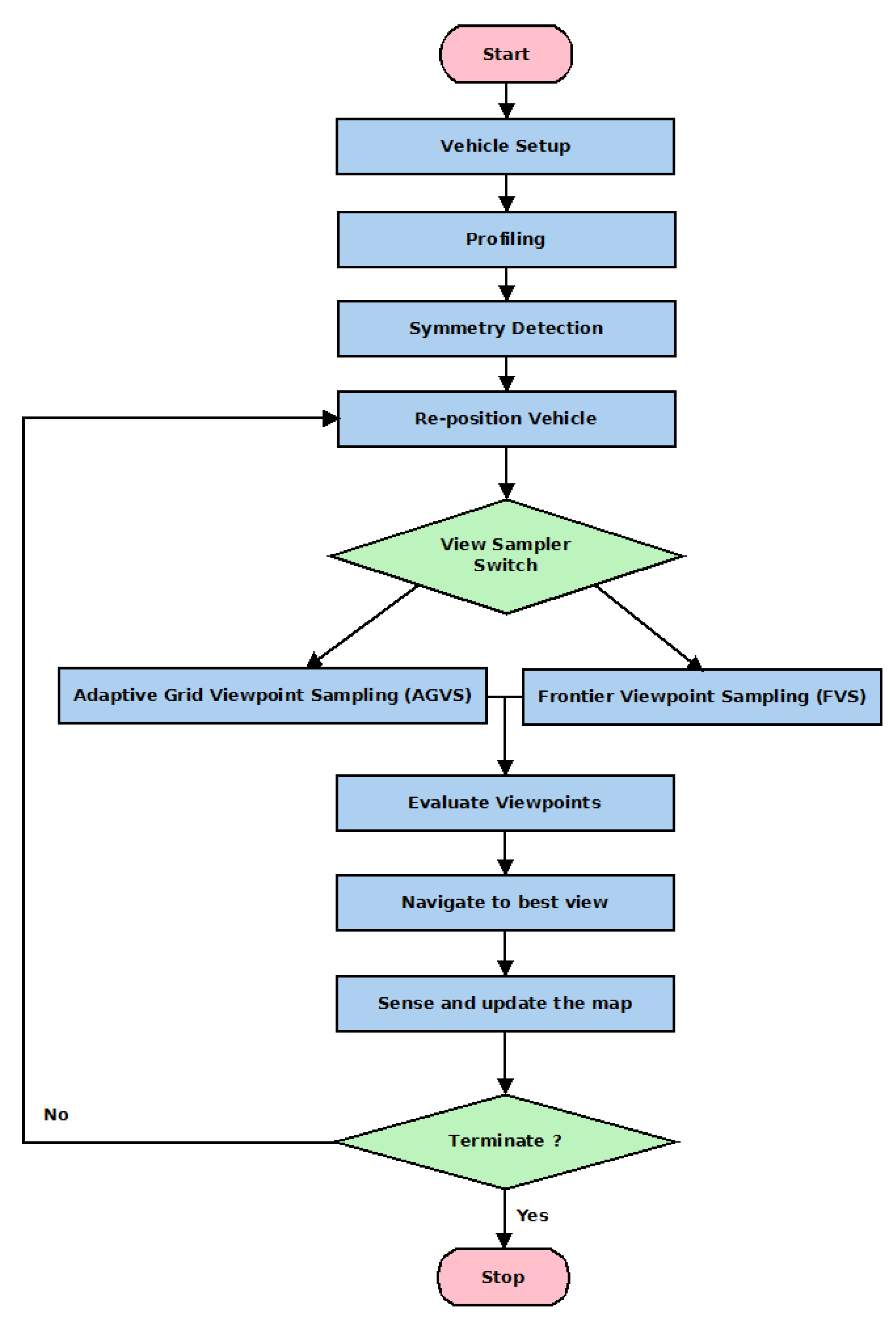
After the profiling process, the standard NBV method steps are performed iteratively, as shown in Figure 1. The method samples a set of viewpoints, which are evaluated to determine the next best viewpoint. The selected viewpoint is then followed by the UAV where it updates the model using the obtained observations. If the termination condition is not satisfied, the process is repeated. Following these steps forms a full iteration of NBV. All of these steps are discussed in details in the next sections.
The system can operate using different number of camera sensors with varying sensor ranges and fields of view. There are two main assumptions used in the proposed system: availability of an accurate global positioning system and a workspace of known dimensions.
2.1. 3D Mapping
The 3D mapping module performs the data acquisition related to the NBV process. This module is also responsible for the 3D mapping associated processes such as density calculations, saving/loading maps and storing the final structure model. Two representations are used in the 3D mapping module processes: a 3D occupancy grid map consisting of voxels (OctoMap) to guide the NBV process and a point cloud for the final 3D reconstruction. The gathered data by the RGBD sensors and LIDAR are used to update these representations at each iteration.
The final model of the object of interest is created using the point cloud data. During the NBV exploration, the point cloud is used to create a 3D occupancy grid using the OctoMap implementation. The collected point cloud is used to generate a 3D model of the object once the mission is completed. Then, the collected images during the NBV exploration can be used to texture the final generated mesh model.
The 3D occupancy grid divides space into a grid of voxels where each voxel is marked with one state as being free (containing no points), occupied (containing points), or unknown. Using the OctoMap, continuous values are stored rather than discrete state in order to determine the likelihood of a voxel being occupied, with likelihood of 0 being free, 1 being occupied, and meaning it could be occupied or free with equal likelihood. Using OctoMap, a set of occupancy and clamping thresholds are defined for the upper and lower bounds of occupancy probabilities to represent the different states and ensure that confidence is bounded. The notion of entropy from information theory is used to determine the amount of remaining information in the scene. The entropy of the voxel i with occupancy probability is computed using Equation (1).
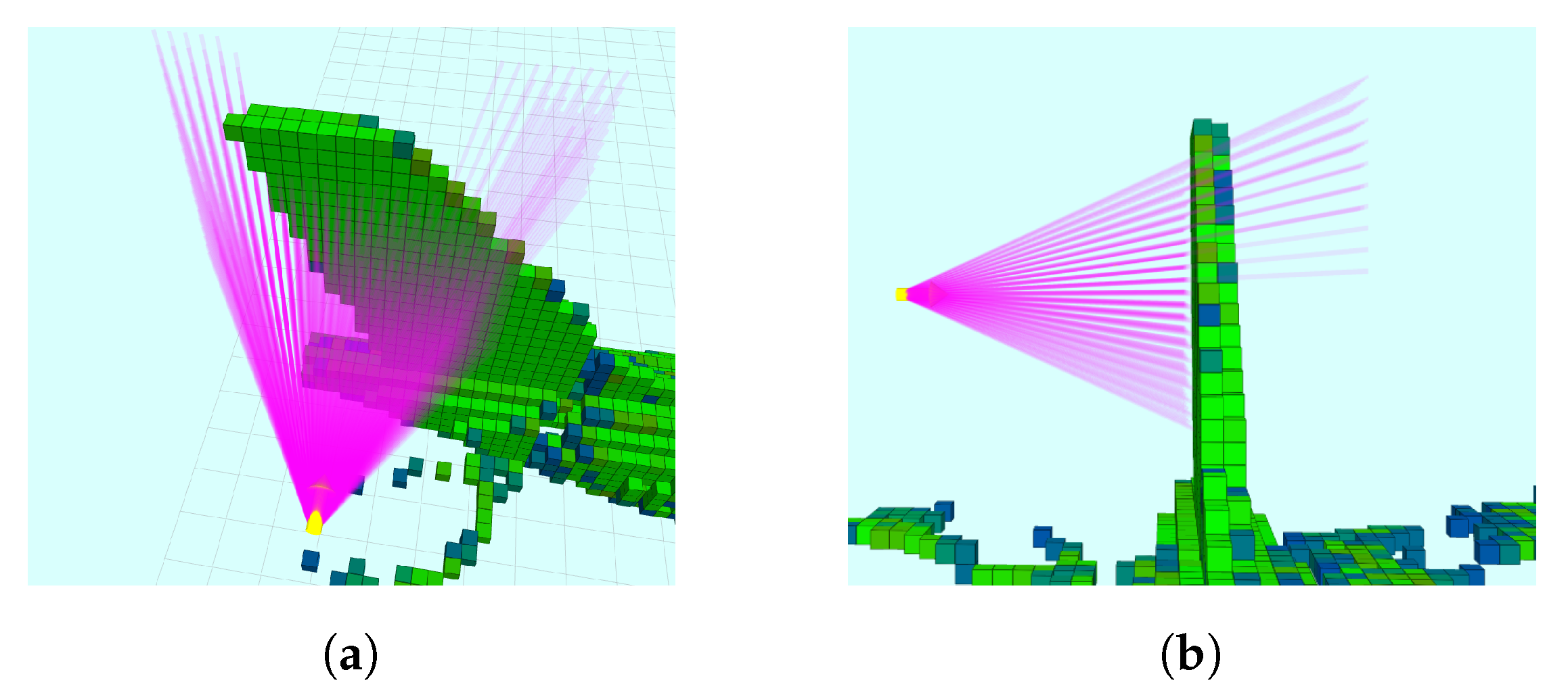
In NBV, the “next best view” has to be determined iteratively at each step. Different sensors could be used in the 3D mapping process, each with different limitations including: resolution, maximum/minimum range and Field Of View (FOV). Considering these limitations, it is possible to quantify the Information Gain (IG) metric, which is the amount of information that a particular view contains. To compute IG, a ray casting process is performed from the candidate viewpoint, as shown in Figure 2.
The occupancy grid is not suitable for reconstructing the final structure since it cannot capture the fine details of the structure being constructed. Instead, point cloud is used to construct the final 3D mesh since it is denser and more precise. However, the occupancy grid is a more efficient data representation that facilitates differentiating between free and unexplored space, essential information for computing IG during the Guided NBV approach.
Point Density
During the final iterations of the Guided NBV, the proposed approach switches from exploration to improving the quality of the reconstruction. This ensures a dense and complete coverage without major gaps in the model. A density measure is included in the proposed method in order to account for this switch.
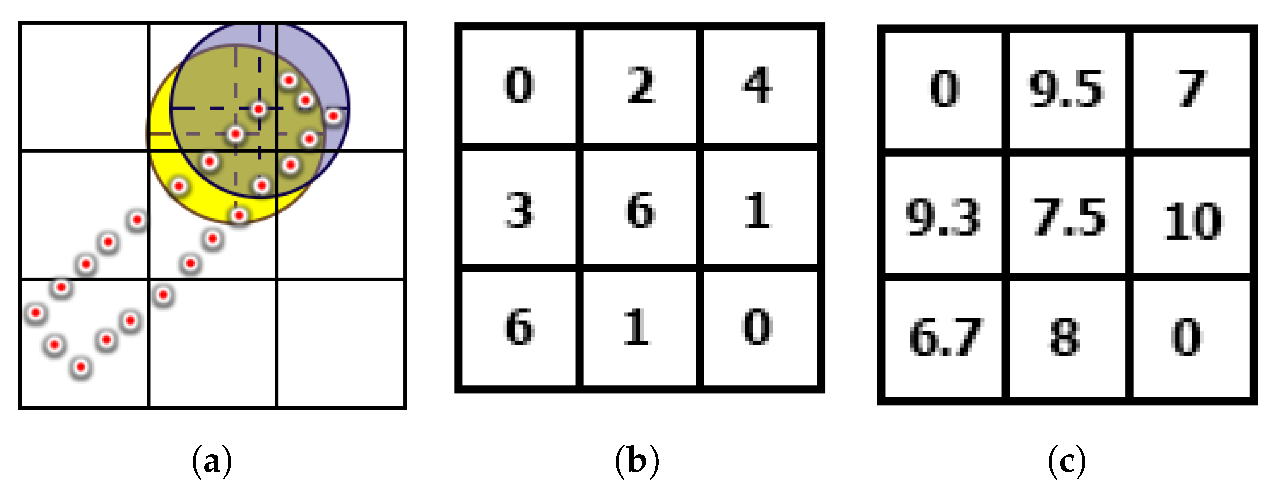
Computing the density by only considering the number of points in each voxel provides poor density estimation for complex structures. Some parts of these structures partially passes through the voxel such as curved areas. This makes the density based frontier viewpoint generator (described in Section 2.4) select these areas consistently even though their density will not change. Therefore, we introduce a new density measurement that considers the neighboring points of each point in the final point cloud. The points’ neighbors are found by performing a search for points within a radius from the point. The computed data are then stored with the 3D occupancy grid, which stores the average density of the points and the number of points in that voxel. A 2D example of calculating the density in each cell is shown in Figure 3.
2.2. Profiling
The main aim of the profiling stage is to generate an initial rough model that can guide further NBV exploration. To capture the profile, a laser range finder is used to perform this initial scan. Although the profile can be obtained using visual data, but structure-from-motion and stereoscopic readings provide poor distance estimation at longer ranges, and require multiple viewpoints in order to compute the position of an observed point. Therefore, the combined distance and angular capabilities of LIDARs allow the system to collect sparse data about a large structure quickly.
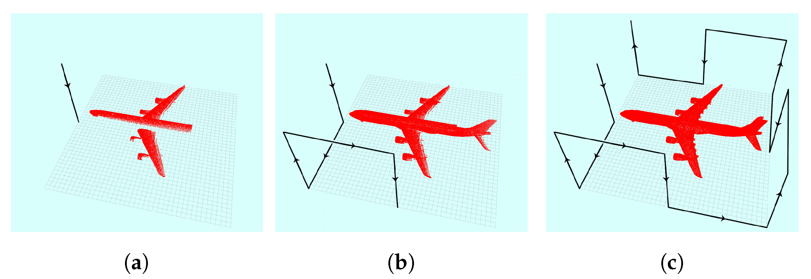
The proposed profile approach creates a suitable path that allows the sensor to move using a set of fixed waypoints on the surface of the structure’s bounded rectangular workspace. This requirement is reasonable in many scenarios since the object being reconstructed is on a known size in a controlled environment. In many cases, the structure is contained within a 3D workspace and occupies finite dimensions. The bounded workspace size can be obtained by either estimation or measurement. Based on the obtained workspace limits, the motion of the sensor is constrained to the bounds of this workspace. The sensor data are gathered and processed as the sensor moves. Updating the occupancy grid is performed by buffering and synchronizing the scan data with the corresponding sensor positions along the trajectory. Once the entire scan is complete, the map is updated in batch using the buffered data. A rectangular bounded box is shown in Figure 4 where the UAV is moved to eight fixed waypoints.
2.3. Exploiting Possible Symmetry
The generated profile may have deficiencies and gaps due to sensor limitations and occlusions. To enhance the obtained structure initial model, the profile can be exploited to make a better prediction by utilizing symmetries that exist in many structures. In this work, reflectional symmetry is utilized, making use of our technique described in [27]. The main steps of symmetry detection described in [27] include: computing keypoints and features in the profile, matching keypoints and fitting planes, determining the symmetry plane using fitted planes, and reflecting a copy of the profile point cloud across line of symmetry. Once the symmetry predicted point cloud is obtained, a new 3D occupancy grid is created using this point cloud with the same resolution and bounds as the main 3D occupancy grid. The areas which consists of predicted points are considered occupied while the rest of the space is assumed to be unknown. Only two states are considered important in the new generated 3D grid: occupied (i.e., predicted) or not. The voxels are expected to be occluded by unseen prediction if the ray length in the predicted 3D grid is shorter than the main 3D map. Using ray-tracing for the purpose of prediction update, the rays are taken to the predictive 3D map where voxels are set to free space if they intersect with the ray. The work presented in [27] explains how symmetry prediction reduces travel cost and improves coverage by correctly predicting unknown cells are part of the surface rather than a large section of an unknown space (given an inflated information gain value).
2.4. Viewpoint Sampling
The process of determining the next best possible viewpoint in a continuous 3D space is intractable, as there an infinite number of possible viewpoints. A few selected viewpoints are sampled, utilizing two proposed approaches: Adaptive Grid Viewpoint Sampling (AGVS) and Frontier Viewpoint Sampling (FVS). The entire Guided NBV process terminates if no more valid candidate viewpoints can be generated. The AGVS viewpoint sampling method is initially used until a local minima is detected based on the entropy change. The viewpoint sampling component switches to FVS, as illustrated in Figure 1, which will direct the robot towards areas with low density. After covering the low density area, the viewpoint sampling switches back to AGVS.
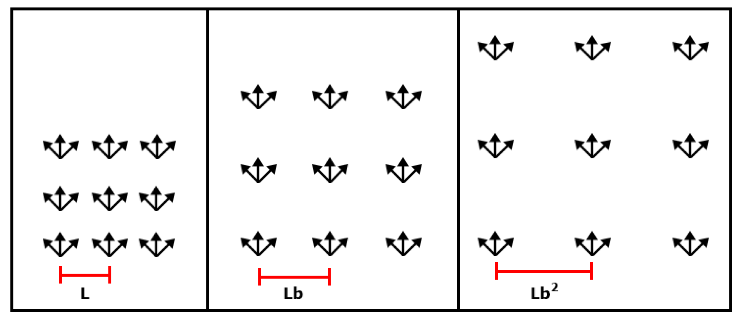
Our AGVS approach described in [27] samples a few viewpoints in the vehicle’s nearby vicinity. It performs position sampling and orientation based sampling . This method reduces travel cost by sampling viewpoints in the nearby vicinity, although it is not globally optimal. Figure 5 shows an example of adaptively generated viewpoints at different scales.
A local minimum is assumed if the maximum entropy change per voxel falls below a threshold within the past few iterations. Therefore, the viewpoint generator switches to FVS, which places the sensor directly in front of regions of interest and frontiers. A frontier is defined in the literature as the boundary between known and unknown space. In our work, frontiers are defined as voxels with low density. By focusing on low density frontiers, obtaining new information is guaranteed. Based on a specified density threshold, a set of frontier voxels is generated. The set of frontiers is clustered using Euclidean based clustering method and the centroid of each cluster is determined. The nearest centroid is then selected to be used in generating the views that fully covers it. The viewpoints are sampled on a cylindrical shape considering the centroid of the cluster as a center. Three layers are generated at different heights from the centroid. Furthermore, four viewpoints are generated at each layer with orientation pointing towards the central axis (the axis passes through the centroid of the cluster). Using three layers around the cluster with viewpoints pointing to the central axis facilitates providing full coverage of the cluster from different directions. This is illustrated in Figure 6.
The validity of viewpoints is checked iteratively as they are generated. The viewpoint is validated by checking if it is in a free space, within workspace bounds, not colliding with octree map, and the centroid is inside its FOV. The visibility of each viewpoint is then obtained in the cylinder utilizing the concept of occlusion culling described in [7] to check the frontier cluster coverage. Occlusion culling process extracts visible points that exist in a viewpoint FOV. The Guided NBV process terminates if all the generated viewpoints by the used method are considered not valid.
2.5. Viewpoint Evaluation
The next best view is determined by selecting the viewpoint that maximizes a utility function. The utility function is computed for each candidate viewpoint using their visible point cloud and occupancy grid. Once the best viewpoint is selected, the vehicle navigates to that viewpoint position, collects data using the mounted sensors, and updates the constructed 3D model accordingly.
The proposed utility function rewards some behaviors and penalizes others. The main objective of our proposed utility function is to maximize the IG, and the density of the final 3D reconstructed model. The utility function also needs to penalize far away viewpoints and utilize the predictions made utilizing the reflectional symmetry feature if it exists. The utility function is calculated for each candidate viewpoint, by evaluating their covered regions, in order to select the best one based on utility value. The proposed utility function formulation is presented in Equation (2) where U is the utility function value, is a normalized expected entropy in the visible candidate region, is a normalized average point density in the visible candidate region, is the number of visible occupied nodes in the visible candidate region, is the normalized ratio of predicted voxels to , d is the Euclidean distance from the current position to the selected viewpoint and , , , and are the weights of each component. The inclusion of each of these terms is described further below.
Information Gain (IG) is often used in the literature [17,28,29], which aims at minimizing the remaining total information by measuring the total entropy of voxels in a given viewpoint’s visible candidate region. The other part is the weighted information gain described in [17], which aims at minimizing euclidean distance d while maximizing the IG. These two parts are combined in our proposed utility function in addition to the other terms.
Viewpoints with high number of occupied voxels are given extra weight in order to direct the vehicle towards areas that overlap with the previous views. This happens when the profile has vast unexplored areas around the structure, which would make the vehicle select unknown voxels that might be away of the structure to maximize information. However, rewarding viewpoints based on high occupied voxels count could lead to the selection of uninformative viewpoints. Therefore, the logarithm is used to avoid this since it rewards increasing magnitudes but does not show significant increase between magnitudes. In our implementation, the base-10 logarithm is used instead of the base-e logarithm since it has a larger interval between magnitudes. This feature facilitates differentiating between viewpoints of extremely low and moderate without rewarding higher excessively. Any higher base-j logarithm can be used in order to further flatten the higher magnitudes effect.
The density is calculated as described previously, utilizing the average number of points in a voxel. The number of predicted voxels is determined by performing ray casting as described in Section 2.3. The prediction ratio is computed using Equation (3), where is the normalized ratio of predicted voxels, is the number of predicted voxels in viewpoint, and is the number of occupied voxels in viewpoint.
2.6. Termination
In general, a suitable termination condition is adapted for each application, but it is difficult to quantify the desired criteria. In ideal scenarios, once the system has achieved coverage completeness, the process should terminate. However, computing coverage percentage without the original reference model is considered difficult. The work presented in [19,30] terminates if no viewpoint has an IG above a predefined threshold while the work in [31] terminates if the difference in total entropy reduction decreased below a predefined threshold. Three termination conditions are used in our Guided NBV method: comparing the current NBV process iteration number with a predefined maximum iterations number, checking the global entropy E change after n iterations [32], or when no valid viewpoints are generated by the viewpoint sampling component. as mentioned previously.
Using global entropy change approach, the process terminates if the condition is satisfied for more than n consecutive iterations. To avoid premature termination if the method is stuck in a local minimum, a sufficient value of n is selected. If the total number of unknown voxels is very large, the values of and will be large and hence the difference will be small. This could happen in large complex structures represented using voxels with small resolution or when the profile quality is not good. Therefore, for large structures, several consecutive iterations need to be selected to check the differences.
The NBV termination conditions related to the viewpoints validity and vehicles motion repetition check are embedded as part of the NBV cycle. The other termination conditions related to the fixed maximum number of iterations and global entropy change are selected based on the application where only one of them is selected. UAVs have limited flight time, which requires selecting a suitable termination method based on the conducted experiment. In practical applications, the maximum number of iterations could be selected based on the complexity of the structure, and the amount of captured information. The amount of captured information at each viewpoint is affected by the number of used sensors and the voxels ray-tracing process.
3. Experimental Results
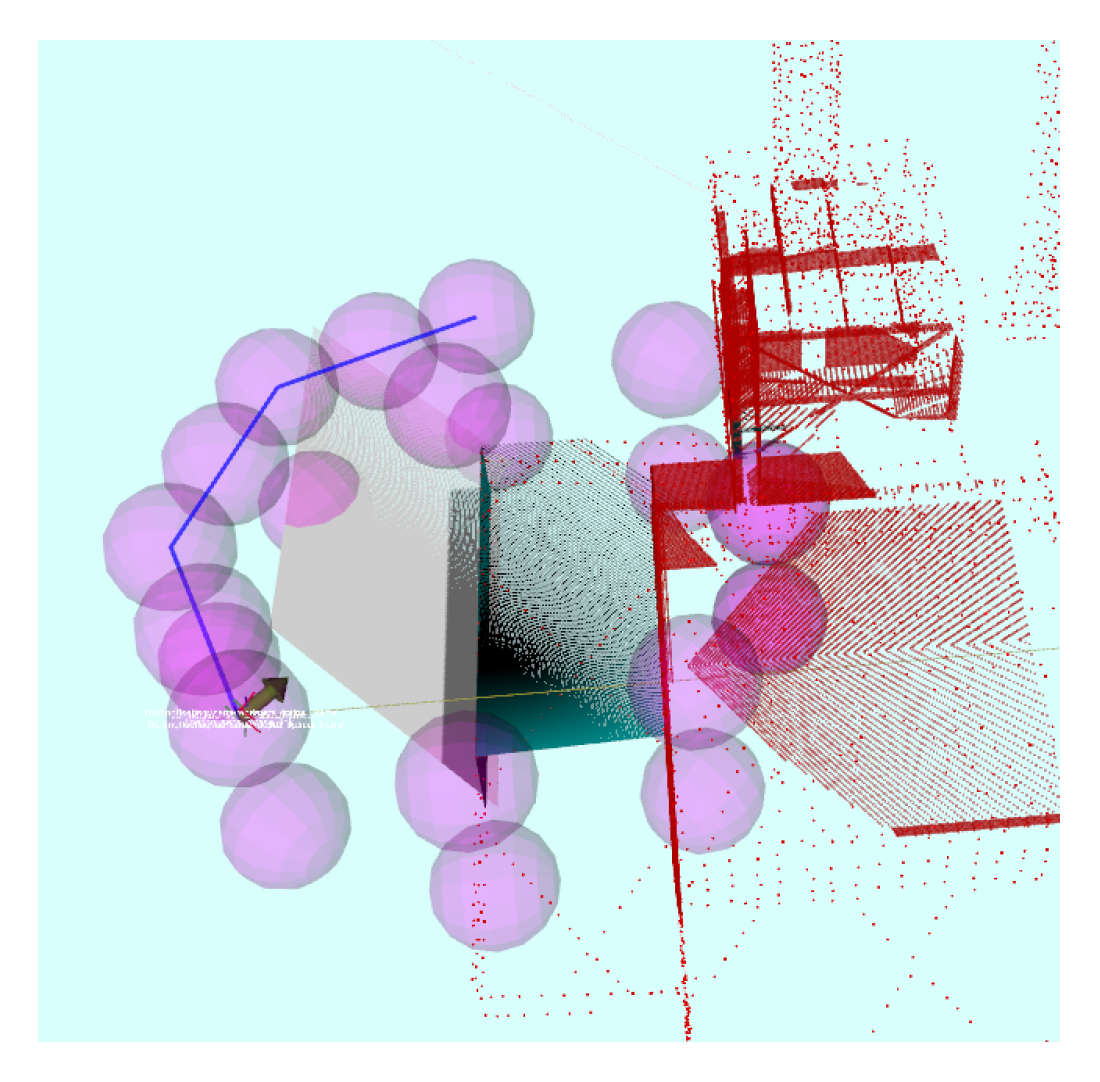
To perform experimental evaluation, four models were selected: an A340 aircraft and a power plant models used in simulation, and a lab representative model and an airplane used for the indoor real experiments. These models represent environments with different geometrical features in terms of shapes, curves, textures, and volumes. Two real indoor experiments were conducted using different structures in order to validate the applicability of the Guided NBV system. In all experiments, collision check with the structure was performed by constructing a circular collision box around the UAV. The motion of the UAV was also constrained within the specified structure workspace dimensions. Figure 7 shows an example of the circular collision box created to check the viewpoints validity. The path connecting the current position with the next candidate viewpoint was also checked for collision, utilizing the generated profile to compute path intersections. If the path intersected with the profile, the viewpoint was discarded and another candidate viewpoint was checked. This allowed avoiding collisions with the structure while following the path connecting viewpoints.
3.1. Simulated Experiments
3.1.1. Simulation Setup
The first two scenarios were Software-In-The-Loop (SITL) [33] experiments using simulated Iris quadrotor platform. The quadrotor consists of RGBD sensors with a range of 0.3–8 m and a laser scanner mounted at around y axis, with FOV of and range of 0.1–30 m. The SITL system uses a PX4 Firmware [33] similar to the real UAV system Firmware. The simulated Firmware and the on board computer communicate through the mavlink protocol using a ROS plugin (mavros) [34]. The 3D occupancy grid was processed and represented using OctoMap library [25], while the processing of the point cloud was performed using the Point Cloud Library [35].
The octree resolution was selected to be 0.2 m for both scenarios since they include complex large structures that have detailed shapes. A collision radius of 1.5 m was selected based on the size of the used quadrotor. For the AGVS view generator, the selected sampling distance was 1 m while the selected sampling angle was to allow the view generator create a variety of possible viewpoints that points to the structure. Table 1 summarizes the other parameters used in the two simulation scenarios. The specified number of vertices and faces of the structures mesh models defines the amount of details each structure contains in addition to coverage problem scale based on the workspace dimensions.
The coverage evaluation was performed by comparing two new occupancy grids where the first was constructed from the final point cloud and the second one from the points sampled from the original mesh. Based on the percentage matching between the two occupancy voxel grids, the coverage percentage was evaluated. Using this approach with different voxel sizes allows measuring two different types of coverage including overall shape coverage (large voxels, e.g., 0.5 m), and detailed shape coverage (small voxels, e.g., 0.05 m). In both scenarios, the proposed Guided NBV was compared against the two state-of-the-art utilities functions, namely weighted IG [17] and total entropy of voxels in viewpoint [29], applying the same parameters for all the experiments.
3.1.2. Simulation Results
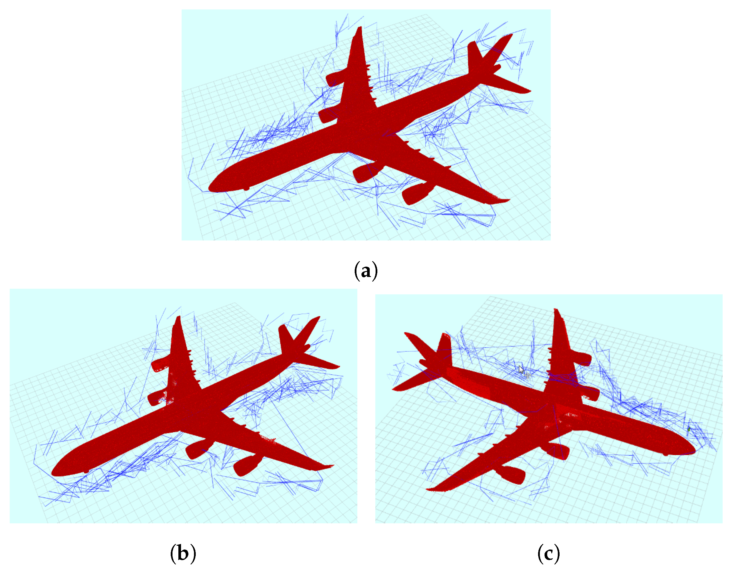
- Aircraft ModelA 3D reconstructed model of an aircraft was generated in this experiment by exploring the bounded box of the structure. A dense point cloud map was generated using the data collected at the selected viewpoints along the generated exploration path in simulation.Figure 8 presents the achieved coverage and the path generated to cover the aircraft model. Table 2 illustrates the results obtained by our proposed method when compared to other two approaches in terms of coverage, distance, and entropy reduction. As shown in the table, the density and resolution of the reconstructed model is low () since the profiling was performed at the edges of the bounded workspace from a long distance. The overall achieved coverage approaches high percentages () and improves the model density when our proposed Guided NBV method was used. Since the aircraft model is symmetric, the utility function weights were selected to achieve high density and utilize the existing prediction measures. Using the proposed utility function with the selected weights, as shown in Table 1, facilitated the capturing of more data by allowing the UAV to travel around the structure more efficiently. The plot shown in Figure 9 illustrates the average density attribute along the iterations for each of the used utility functions. As shown in the plot, the proposed utility function achieves higher density values per voxel in each iteration than the other two approaches. The plot is non-monotonic since the average density was computed based on the size of point cloud and the number of occupied voxels in the octree. At complex curved areas, some voxels hold few points compared to other voxels, which creates the difference in the average density. The details of the structure were captured with high coverage density when evaluated with voxels of resolution 0.05 m. However, this achieved improvement in coverage comes at a cost which is an increase in the traveled distance.
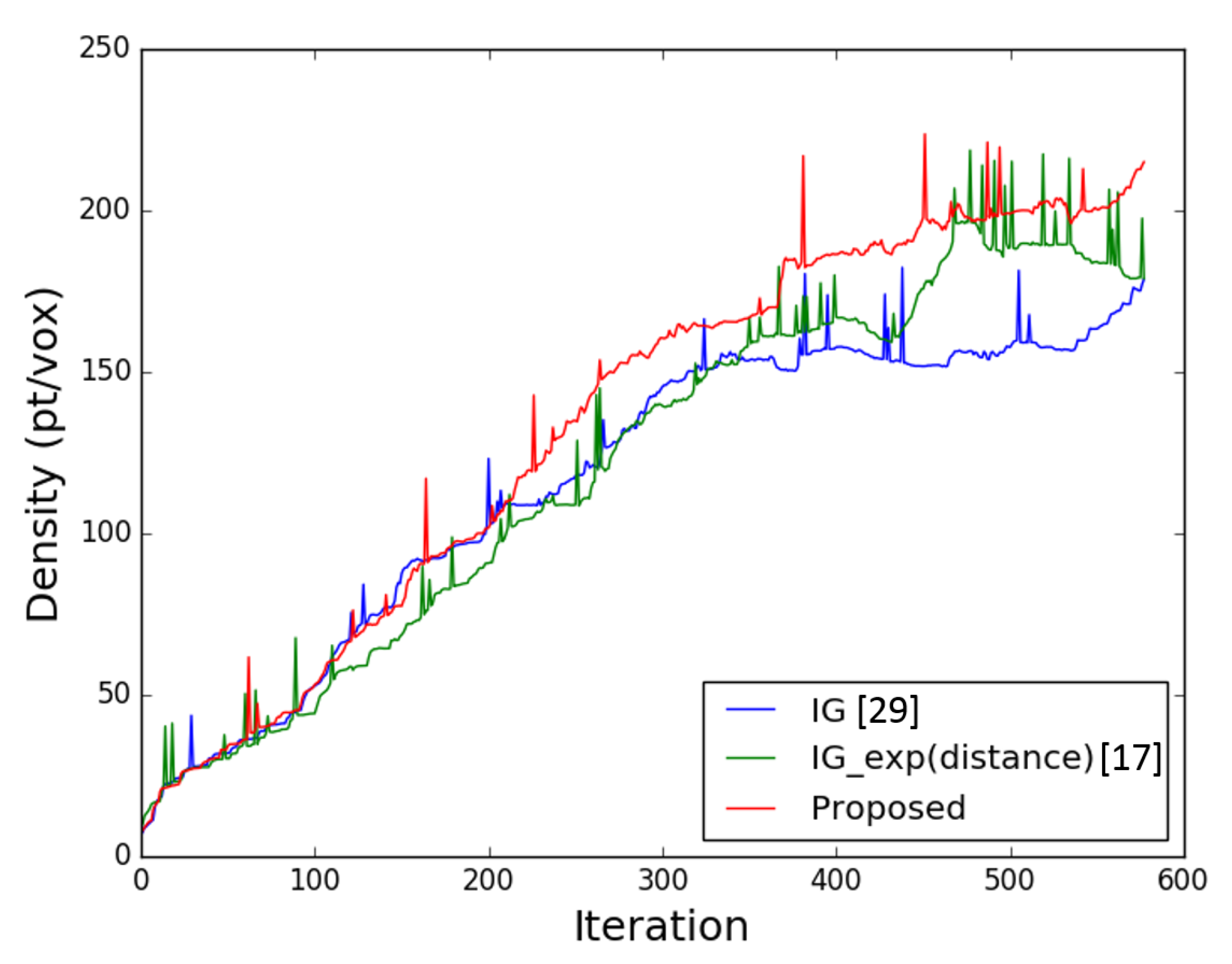
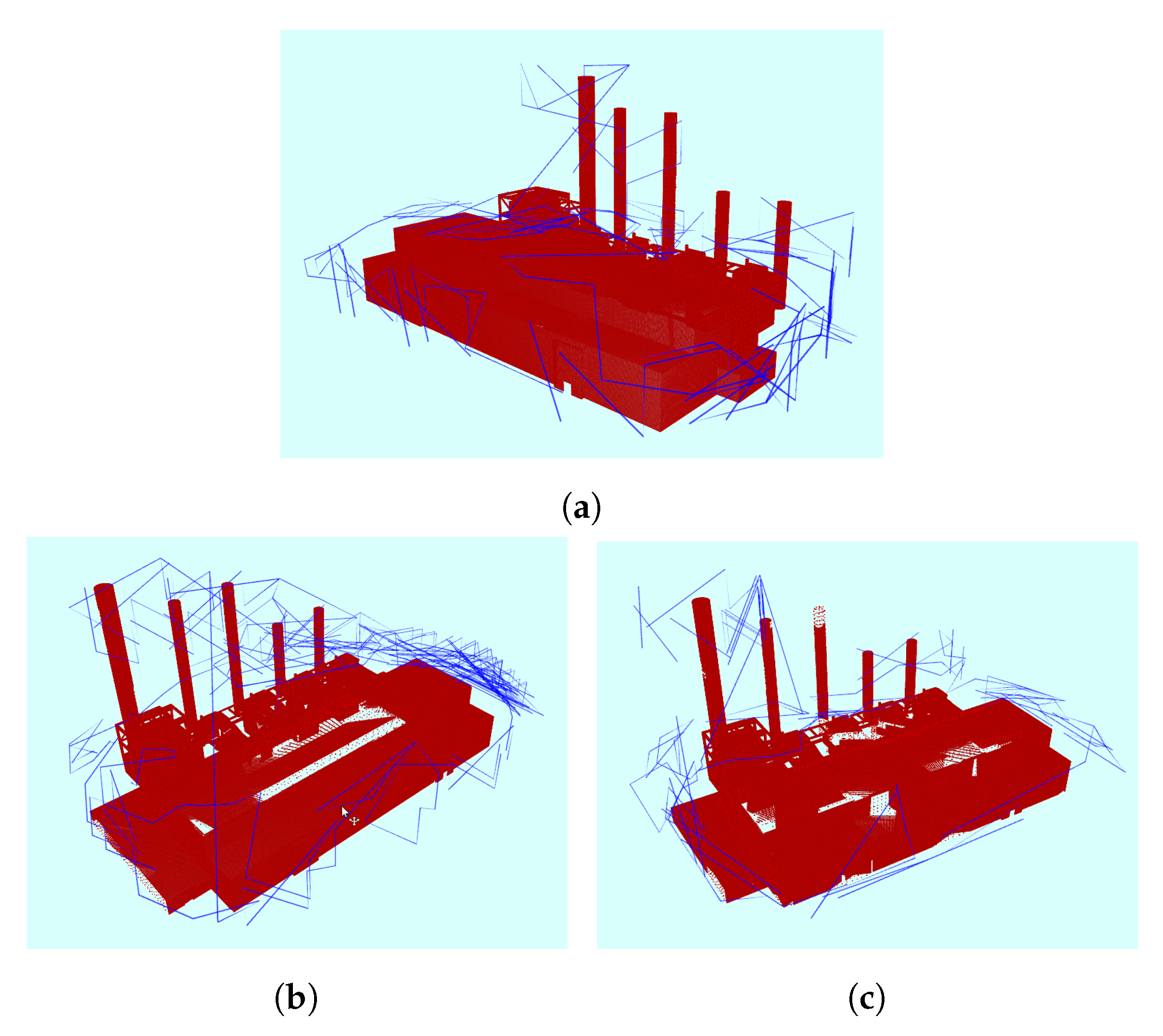
- Power Plant ModelSimilarly, the power plant structure was 3D reconstructed by exploring the bounded box of the model workspace. The collected data at each viewpoint in simulation were used to generate a dense point cloud map. The generated paths and achieved coverage are shown in Figure 10, and the results compared with two other approaches are illustrated in Table 3. As shown in the table, the resolution and density of the reconstructed structure is low ().The Guided NBV achievesd high coverage percentages compared to the two other illustrated approaches. The longer path distance is compensated by a better coverage percentage and average density (proposed density = 177 pt/voxel, Bircher et al. [17] = 140 pt/voxel, Isler et al. [29] = 152 pt/voxel). Moreover, the Guided NBV achieves high coverage () for the power plant structure compared to Song and Jo [21] () and Song and Jo [21] () using similar setup and structure model.The power plant model is not symmetric, thus the utility function weights were selected to achieve high density, as shown in Table 1. The plot shown in Figure 11 illustrates the average density and entropy attributes along the iterations showing the FVS effect on the reduction of the entropy and the increase of the density at some areas. Using the AGVS sampling method with FVS facilitated dense coverage, exceeding . This is mainly due to the ability to take larger steps to escape local minima.
3.2. Real Experiments
3.2.1. Real Experiment Setup
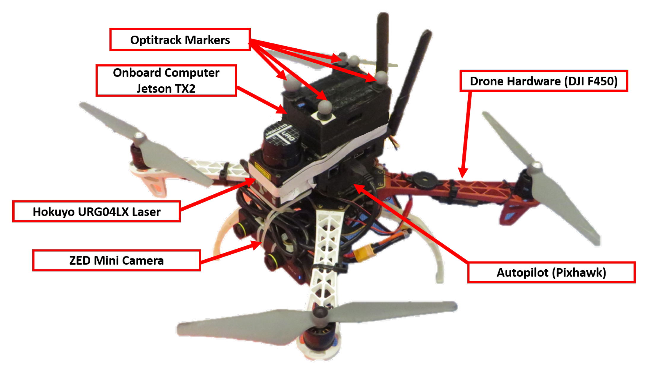
The third and fourth scenarios were performed in an indoor lab environment using a UAV platform. A quadrotor based frame was used with a Pixhawk autopilot system running PX4 Firmware [33]. A Jetson TX2 onboard computer is mounted on the quadrotor running the Guided NBV process, and it is connected to the autopilot system via mavlink protocol [34]. A ZED Mini camera of a FOV () is mounted on the quadrotor with a tilt angle, at m along the z-axis. A hokuyo LIDAR is mounted on the quadrotor for profiling at m along the z-axis. The position of the quadrotor is determined using an Optitrack motion capture system [36]. Figure 12 shows the quadrotor utilized in this experiment.
A collision radius of m was selected based on the size of the DJI 450. For the AGVS viewpoints generator, the selected sampling distance was m while the selected sampling angle was . These viewpoints generator parameters were selected to facilitate the generation of a set of possible viewpoints within the indoor lab workspace dimensions. The utility function weights were selected also to be as . A fixed number of iterations was selected as the termination condition. Table 4 summarizes the other parameters used in the two real experiments scenarios.
Offline 3D reconstruction of the selected structures was performed using the collected images during the Guided NBV exploration. While the UAV was exploring the environments, an OctoMap was generated using the processed point cloud.
3.2.2. Real Experiment Results
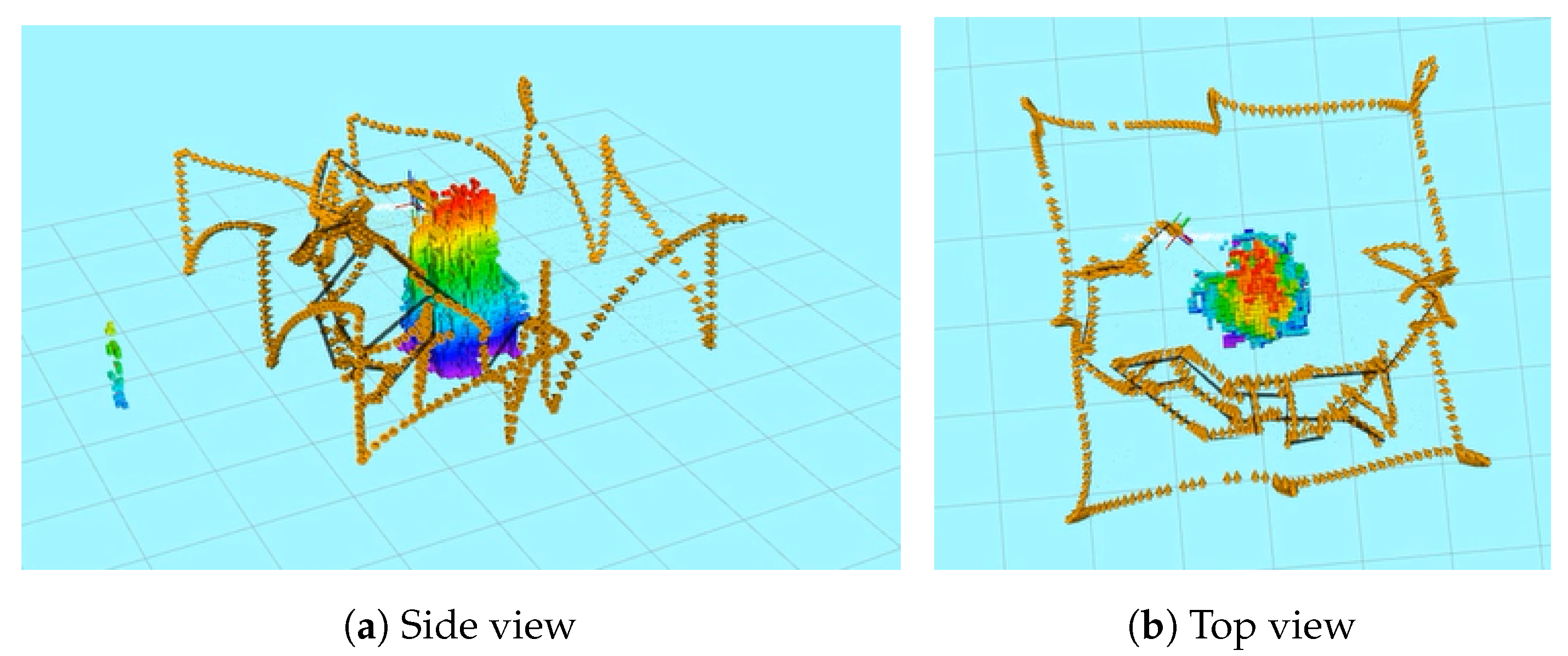
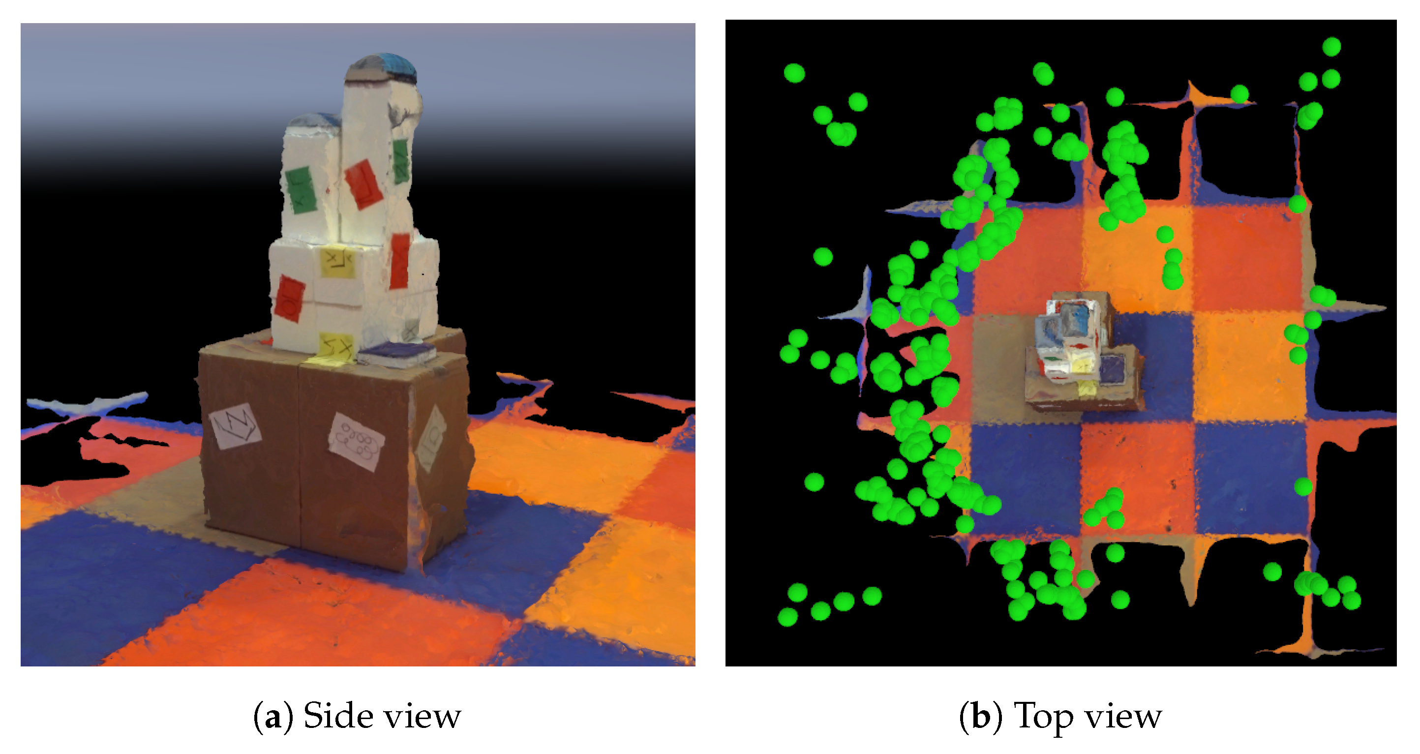
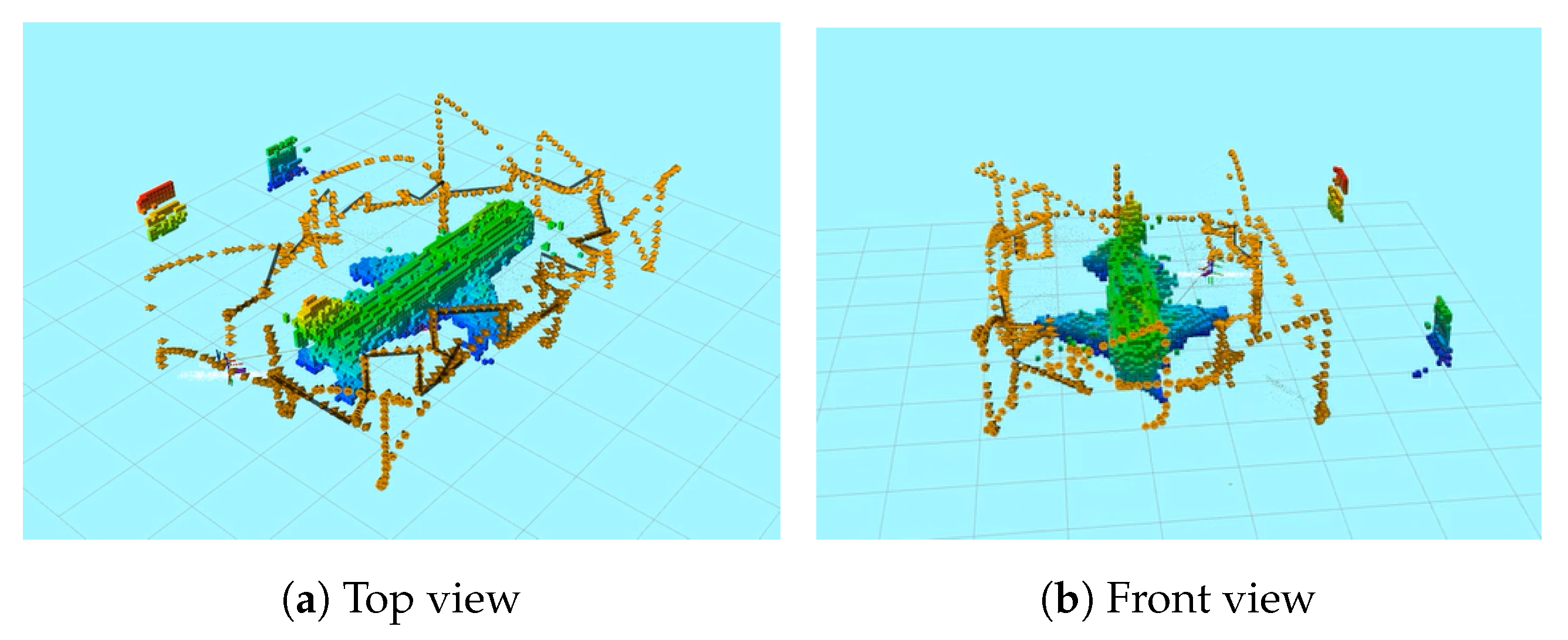
- Representative ModelA representative model in an indoor lab environment was used in this experiment. The proposed Guided NBV was performed starting with a profiling stage, and then executing the NBV iterative process using quadrotor platform, as described previously. The generated exploration path is shown in Figure 13, which consists of 40 viewpoints, with a path length of 32 m, generated in min. The obtained average density is 33 points/voxel and the entropy reduction value is . The plot shown in Figure 14 shows the decreasing entropy and increasing density behaviors across the iterations.A feasible exploration path was generated by our proposed Guided NBV approach for the indoor structure. This is demonstrated in the 3D OctoMap (resolution of m) of the structure, which was generated while exploring the environment using the real quadrotor UAV platform and collecting data along the path. The final textured 3D reconstructed model is shown in Figure 15. Trajectory planning could be performed to connect the waypoints optimizing the path for the UAV acceleration or velocity as a further enhancement. The illustration of the indoor lab experiment of Scenario 3 is shown in a video at [37].
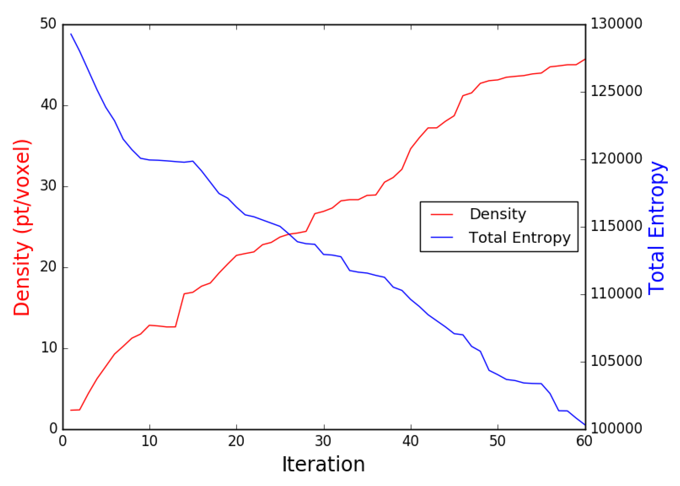
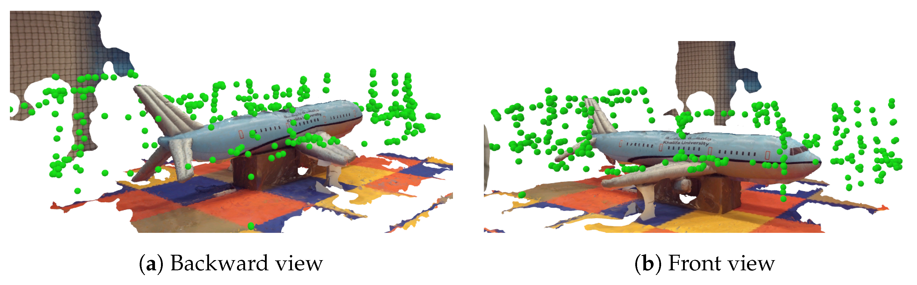
- Airplane ModelIn this experiment, another model of different complexity in terms of shape and texture was selected which is the airplane. The generated exploration path is shown in Figure 16 and it consists of 60 waypoints, with a path length of m, generated in min. Figure 17 shows the plot of the obtained increasing average density and decreasing entropy with an average density of 45 points/voxel and entropy reduction value is 28949.The achieved results show the applicability of our proposed NBV exploration method to different structures, which can be illustrated in the generated 3D OctoMap (resolution of ) of the airplane structure. A finer OctoMap resolution was used since the airplane consists of more details and edges than the previous representative model. The final textured 3D reconstructed model of the airplane is shown in Figure 18. The illustration of the indoor lab experiment of Scenario 4 is shown in a video at [38].
4. Discussion
Using our proposed Guided NBV facilitates exploring unknown structures to provide 3D reconstructed model that can be used for different purposes such as inspection. Experiments were performed using different structures of interest to demonstrate the effectiveness of the Guided NBV. According to the obtained results from simulated structures, the Guided NBV generated feasible paths for the aircraft model, and power plant model. This was demonstrated in the final dense point cloud map, which can be further used to generate a 3D reconstructed model. The proposed approach was applied on symmetric and not symmetric structures by modifying the proposed utility function weights accordingly. The achieved results were compared with two other utility functions, which showed reconstructed models with low density and resolution compared to our final reconstructed model. Our proposed FVS facilitated escaping local minima by taking large steps, which increased density and reduced entropy. The paths connecting the viewpoints that cover frontiers affect the utility since they are located in different locations when the coverage reach high percentages. In addition, the path needs to avoid colliding with the structure. This effect is controlled using the penalizing distance factor parameter. Although covering frontiers with low density increases the traveled distance, it allows achieving higher density and coverage of the structure.
The proposed Guided NBV was also validated in a real indoor environment using representative model and airplane model. Using a real quadrotor platform, the Guided NBV generated exploration paths for both models demonstrating their feasibility in the final generated 3D OctoMap and 3D textured model. The collected images along the path could be used to enhance the texture of the final reconstruction in simulated experiments. The generated path could be further enhanced by performing trajectory planning optimizing the path between the waypoints considering the UAV motion constraints including velocity and acceleration.
5. Conclusions
In this paper, a Guided NBV approach is proposed to explore unknown large structures and 3D reconstruct them. Our approach facilitates the practical deployment of UAVs in reconstruction and inspection applications when a model of the structure is not known a priori. Our proposed NBV starts with an initial scanning step called profiling that facilitates the NBV process. Our main contributions with respect to the state-of-the-art include: a density frontier based viewpoint generator, an adaptive based viewpoint generator that avoids local minima, and a novel utility function. The four main components of the proposed utility function are information gain, distance, density and symmetry prediction. The total remaining information is minimized using the information theory approach, while the travel cost is minimized by the distance component. The density component facilitates generating final dense 3D model. A set of simulations and real indoor experiments were performed with structures of different shapes and complexities. The achieved results demonstrate that our proposed approach improves coverage completeness, density and entropy reduction compared to the other state-of-the-art approaches. The implementation of the proposed algorithm is accessible in [26]. For the future work, the proposed method will be extended to use multi-agent systems and to use deep reinforcement learning to detect occluded parts accurately. The view selection will also be extended to consider the energy of the UAV and the covered surface area. The trajectory of the UAV will be enhanced by performing trajectory planning considering the UAV motion constraints.
Author Contributions
Methodology, R.A., A.A. and T.T.; Software, R.A., A.A. and T.T.; Supervision, T.T., L.S. and Y.Z.; Validation, R.A.; Writing—original draft, R.A.; and Writing—review and editing, R.A., T.T. and Y.Z.
Funding
This research received no external funding.
Acknowledgments
This publication was based on work supported by the Khalifa University of Science and Technology under Award No. RC1-2018-KUCARS.
Conflicts of Interest
The authors declare no conflict of interest.
References
- Faria, M.; Maza, I.; Viguria, A. Applying Frontier Cells Based Exploration and Lazy Theta* Path Planning over Single Grid-Based World Representation for Autonomous Inspection of Large 3D Structures with an UAS. J. Intell. Robot. Syst. 2019, 93, 113–133. [Google Scholar] [CrossRef]
- Hollinger, G.A.; Englot, B.; Hover, F.S.; Mitra, U.; Sukhatme, G.S. Active planning for underwater inspection and the benefit of adaptivity. Int. J. Robot. Res. 2013, 32, 3–18. [Google Scholar] [CrossRef]
- Jiang, S.; Jiang, W.; Huang, W.; Yang, L. UAV-Based Oblique Photogrammetry for Outdoor Data Acquisition and Offsite Visual Inspection of Transmission Line. Remote Sens. 2017, 9, 278. [Google Scholar] [CrossRef]
- Oleynikova, H.; Taylor, Z.; Siegwart, R.; Nieto, J. Safe Local Exploration for Replanning in Cluttered Unknown Environments for Micro-Aerial Vehicles. In Proceedings of the IEEE International Conference on Robotics and Automation (ICRA’18), Brisbane, Australia, 21–25 May 2018. [Google Scholar]
- Environments, L.S.; Selin, M.; Tiger, M.; Duberg, D.; Heintz, F.; Jensfelt, P. Efficient Autonomous Exploration Planning of Large-Scale 3-D Environments. IEEE Robot. Autom. Lett. 2019, 4, 1699–1706. [Google Scholar] [Green Version]
- Bircher, A.; Kamel, M.; Alexis, K.; Burri, M.; Oettershagen, P.; Omari, S.; Mantel, T.; Siegwart, R. Three-dimensional coverage path planning via viewpoint resampling and tour optimization for aerial robots. Auton. Robot. 2015, 40, 1059–1078. [Google Scholar] [CrossRef]
- Almadhoun, R.; Taha, T.; Seneviratne, L.; Dias, J.; Cai, G. GPU accelerated coverage path planning optimized for accuracy in robotic inspection applications. In Proceedings of the 2016 IEEE 59th International Midwest Symposium on Circuits and Systems (MWSCAS), Abu Dhabi, UAE, 16–19 October 2016; pp. 1–4. [Google Scholar]
- Frías, E.; Díaz-Vilariño, L.; Balado, J.; Lorenzo, H. From BIM to Scan Planning and Optimization for Construction Control. Remote Sens. 2019, 11, 1963. [Google Scholar] [CrossRef]
- Martin, R.A.; Rojas, I.; Franke, K.; Hedengren, J.D. Evolutionary View Planning for Optimized UAV Terrain Modeling in a Simulated Environment. Remote Sens. 2016, 8, 26. [Google Scholar] [CrossRef]
- Vasquez-Gomez, J.I.; Sucar, L.E.; Murrieta-Cid, R.; Herrera-Lozada, J.C. Tree-based search of the next best view/state for three-dimensional object reconstruction. Int. J. Adv. Robot. Syst. 2018, 15, 1–11. [Google Scholar] [CrossRef]
- Palomeras, N.; Hurtos, N.; Carreras, M.; Ridao, P. Autonomous Mapping of Underwater 3-D Structures: From view planning to execution. In Proceedings of the IEEE International Conference on Robotics and Automation (ICRA’18), Brisbane, Australia, 21–25 May 2018; pp. 1965–1971. [Google Scholar]
- Martin, R.A.; Blackburn, L.; Pulsipher, J.; Franke, K.; Hedengren, J.D. Potential Benefits of Combining Anomaly Detection with View Planning for UAV Infrastructure Modeling. Remote Sens. 2017, 9, 434. [Google Scholar] [CrossRef]
- Shade, R.; Newman, P. Choosing where to go: Complete 3D exploration with stereo. In Proceedings of the 2011 IEEE International Conference on Robotics and Automation (ICRA), Shanghai, China, 9–13 May 2011; pp. 2806–2811. [Google Scholar]
- Heng, L.; Gotovos, A.; Krause, A.; Pollefeys, M. Efficient visual exploration and coverage with a micro aerial vehicle in unknown environments. In Proceedings of the 2015 IEEE International Conference on Robotics and Automation (ICRA), Seattle, WA, USA, 26–30 May 2015; pp. 1071–1078. [Google Scholar]
- Haner, S.; Heyden, A. Discrete Optimal View Path Planning. In Proceedings of the 10th International Conference on Computer Vision Theory and Applications (VISAPP 2015), Berlin, Germany, 11–14 March 2015; pp. 411–419. [Google Scholar]
- Cieslewski, T.; Kaufmann, E.; Scaramuzza, D. Rapid exploration with multi-rotors: A frontier selection method for high speed flight. In Proceedings of the 2017 IEEE/RSJ International Conference on Intelligent Robots and Systems (IROS), Vancouver, BC, Canada, 24–28 September 2017; pp. 2135–2142. [Google Scholar]
- Bircher, A.; Kamel, M.; Alexis, K.; Oleynikova, H.; Siegwart, R. Receding Horizon “Next-Best-View” Planner for 3D Exploration. In Proceedings of the 2016 IEEE International Conference on Robotics and Automation (ICRA), Stockholm, Sweden, 16–21 May 2016; pp. 1462–1468. [Google Scholar]
- Oshima, S.; Nagakura, S.; Yongjin, J.; Kawamura, A.; Iwashita, Y.; Kurazume, R. Automatic planning of laser measurements for a large-scale environment using CPS-SLAM system. In Proceedings of the 2015 IEEE/RSJ International Conference on Intelligent Robots and Systems (IROS), Hamburg, Germany, 28 September–3 October 2015; pp. 4437–4444. [Google Scholar]
- Palomeras, N.; Hurtos, N.; Vidal Garcia, E.; Carreras, M. Autonomous exploration of complex underwater environments using a probabilistic Next-Best-View planner. IEEE Robot. Autom. Lett. 2019. [Google Scholar] [CrossRef]
- Palazzolo, E.; Stachniss, C. Effective Exploration for MAVs Based on the Expected Information Gain. Drones 2018, 2, 9. [Google Scholar] [CrossRef]
- Song, S.; Jo, S. Surface-based Exploration for Autonomous 3D Modeling. In Proceedings of the IEEE International Conference on Robotics and Automation (ICRA’18), Brisbane, Australia, 21–25 May 2018; pp. 4319–4326. [Google Scholar]
- Song, S.; Jo, S. Online inspection path planning for autonomous 3D modeling using a micro-aerial vehicle. In Proceedings of the IEEE International Conference on Robotics and Automation, Singapore, 29 May–3 June 2017; pp. 6217–6224. [Google Scholar]
- Hepp, B.; Nießner, M.; Hilliges, O. Plan3D: Viewpoint and Trajectory Optimization for Aerial Multi-View Stereo Reconstruction. ACM Trans. Graph. 2017, 38, 4:1–4:17. [Google Scholar] [CrossRef]
- Roberts, M.; Dey, D.; Truong, A.; Sinha, S.N.; Shah, S.; Kapoor, A.; Hanrahan, P.; Joshi, N. Submodular Trajectory Optimization for Aerial 3D Scanning. In Proceedings of the 2017 IEEE International Conference on Computer Vision (ICCV), Venice, Italy, 22–29 October 2017; pp. 5334–5343. [Google Scholar]
- Hornung, A.; Wurm, K.M.; Bennewitz, M.; Stachniss, C.; Burgard, W. OctoMap: An efficient probabilistic 3D mapping framework based on octrees. Auton. Robot. 2013, 34, 189–206. [Google Scholar] [CrossRef]
- Source Implementation Package of the Proposed Algorithm. Available online: https://github.com/kucars/ma_nbv_cpp.git (accessed on 30 May 2018).
- Abduldayem, A.; Gan, D.; Seneviratne, L.; Taha, T. 3D Reconstruction of Complex Structures with Online Profiling and Adaptive Viewpoint Sampling. In Proceedings of the International Micro Air Vehicle Conference and Flight Competition, Malaga, Spain, 14–16 June 2017; pp. 278–285. [Google Scholar]
- Holz, D.; Basilico, N.; Amigoni, F.; Behnke, S. Evaluating the efficiency of frontier-based exploration strategies. In Proceedings of the ISR 2010 (41st International Symposium on Robotics) and ROBOTIK 2010 (6th German Conference on Robotics), Munich, Germany, 7–9 June 2010. [Google Scholar]
- Isler, S.; Sabzevari, R.; Delmerico, J.; Scaramuzza, D. An information gain formulation for active volumetric 3D reconstruction. In Proceedings of the 2016 IEEE International Conference on Robotics and Automation (ICRA), Stockholm, Sweden, 16–20 May 2016; pp. 3477–3484. [Google Scholar]
- Quin, P.; Paul, G.; Alempijevic, A.; Liu, D.; Dissanayake, G. Efficient neighbourhood-based information gain approach for exploration of complex 3d environments. In Proceedings of the 2013 IEEE International Conference on Robotics and Automation (ICRA), Karlsruhe, Germany, 6–10 May 2013; pp. 1343–1348. [Google Scholar]
- Paul, G.; Webb, S.; Liu, D.; Dissanayake, G. Autonomous robot manipulator-based exploration and mapping system for bridge maintenance. Robot. Auton. Syst. 2011, 59, 543–554. [Google Scholar] [CrossRef] [Green Version]
- Abduldayem, A.A. Intelligent Unmanned Aerial Vehicles for Inspecting Indoor Complex Aero-Structures. Master’s Thesis, Khalifa University, Abu Dhabi, UAE, 2017. [Google Scholar]
- PX4. Available online: http://px4.io/ (accessed on 16 July 2019).
- Mavros. Available online: http://wiki.ros.org/mavros (accessed on 16 July 2019).
- Rusu, R.B.; Cousins, S. 3D Is Here: Point Cloud Library (PCL). In Proceedings of the IEEE International Conference on Robotics and Automation (ICRA), Shanghai, China, 9–13 May 2011. [Google Scholar]
- Optitrack. Available online: http://www.optitrack.com/ (accessed on 25 March 2019).
- Experimentation Using Representative Model. Available online: https://youtu.be/fEtUjW0PNrA (accessed on 25 March 2019).
- Experimentation Using Airplane Model. Available online: https://youtu.be/jNX78Iyfg2Q (accessed on 25 March 2019).
Figure 1.
A flowchart of the proposed Guided Next Best View (NBV) method.

Figure 2.
The process of ray tracing. The rays are shown in pink, occupied voxels are green, free voxels are transparent, and unknown voxels are blue. (a) Virtual rays are casted from the selected viewpoint (shown in yellow) while respecting the sensor limitations. (b) The rays traverse the occupancy map until either the ray reaches the sensor’s maximum range, or the ray is blocked by an occupied cell.

Figure 3.
A 2D example illustrating the cell density calculation method. (a) Cells are represented as a 2D grid, where points in each cell are presented as red dots, and circles illustrate the neighborhood of two-point samples. (b) The classical method for computing density, where the density is simply the number of point in each grid. (c) The density calculated using the proposed method, where a neighborhood search is performed for each point to get a better density estimation.

Figure 4.
Profiling process following structure bounded box. The cumulative profile and path are shown after executing: (a) one waypoint; (b) three waypoints; and (c) eight waypoints.
Figure 4.
Profiling process following structure bounded box. The cumulative profile and path are shown after executing: (a) one waypoint; (b) three waypoints; and (c) eight waypoints.

Figure 5.
Example of AGVS performed using different scale values of , , and , respectively, multiplied by the discretization length L.
Figure 5.
Example of AGVS performed using different scale values of , , and , respectively, multiplied by the discretization length L.

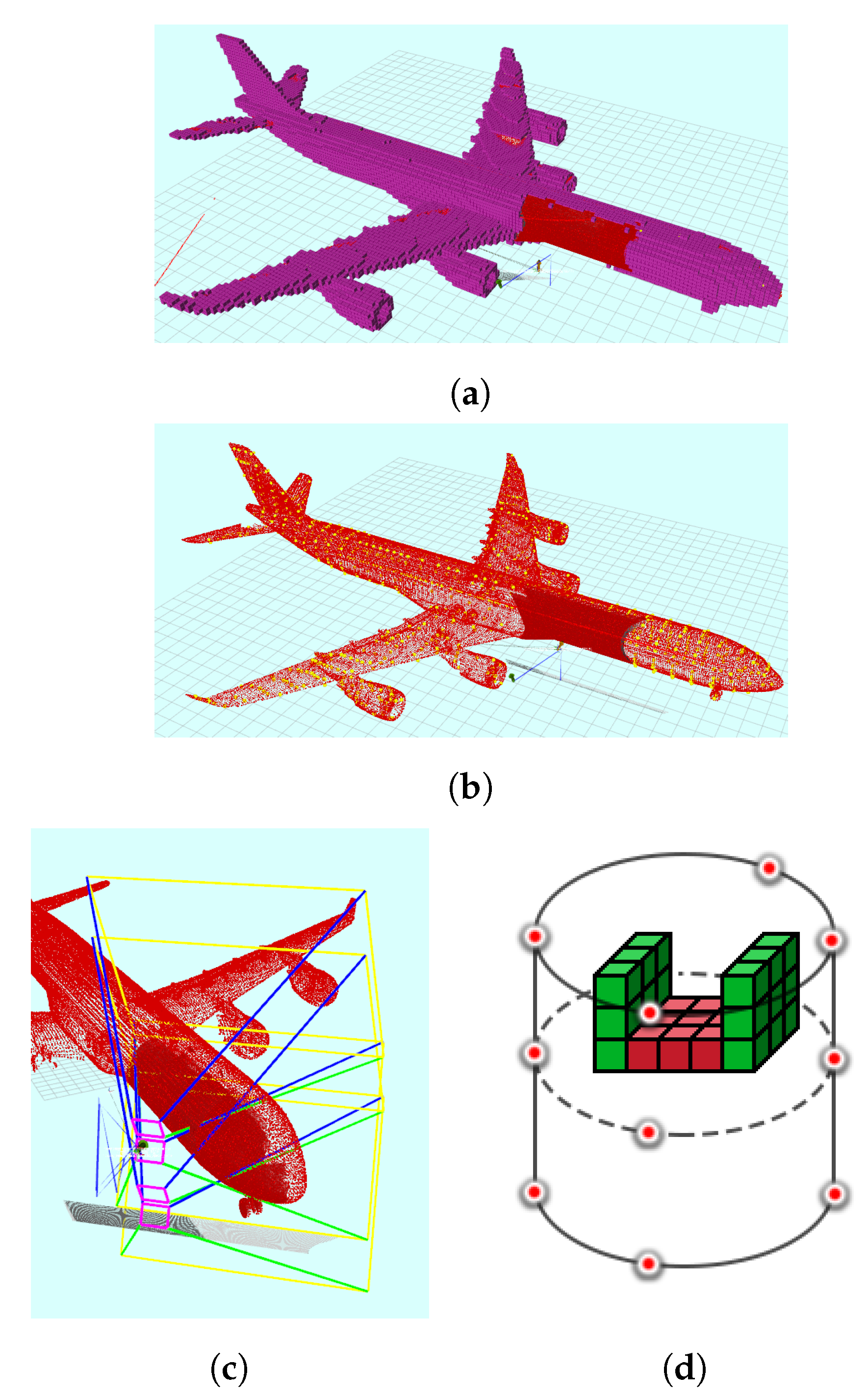
Figure 6.
(a) Low density frontier voxels shown in purple; (b) the centroids (yellow) of the clusters of the frontiers voxels; (c) FOV planes visualization where two sensors are mounted on the UAV; and (d) an example of the three layers to cover an example frontier voxels (cubes) cluster.
Figure 6.
(a) Low density frontier voxels shown in purple; (b) the centroids (yellow) of the clusters of the frontiers voxels; (c) FOV planes visualization where two sensors are mounted on the UAV; and (d) an example of the three layers to cover an example frontier voxels (cubes) cluster.

Figure 7.
The circular collision box in purple created around the UAV locations to check the validity of the viewpoints. The path of the UAV is shown in blue and the scans are presented in dark red.
Figure 7.
The circular collision box in purple created around the UAV locations to check the validity of the viewpoints. The path of the UAV is shown in blue and the scans are presented in dark red.

Figure 8.
The path followed by the UAV in simulation around the aircraft model using three different utility functions: (a) our proposed utility; (b) Isler et al. [29] utility; and (c) Bircher et al. [17] utility.

Figure 9.
The voxel point density vs. the number iterations, showing the proposed approach’s performance as compared to other state-of-the-art utility functions.
Figure 9.
The voxel point density vs. the number iterations, showing the proposed approach’s performance as compared to other state-of-the-art utility functions.

Figure 10.
The path followed by the UAV in simulation around the power plant structure using three different utility functions: (a) our proposed utility; (b) Isler et al. [29] utility; and (c) Bircher et al. [17] utility.

Figure 11.
The density and total entropy attributes along the iterations during the power plant coverage using the proposed Guided NBV. The areas where the viewpoints generator switched to FVS are shown in green.
Figure 11.
The density and total entropy attributes along the iterations during the power plant coverage using the proposed Guided NBV. The areas where the viewpoints generator switched to FVS are shown in green.

Figure 12.
The quadrotor hardware components.

Figure 13.
The path followed by the UAV shown in orange color including the profiling stage. The planned trajectory is shown in black and the reconstruction of the processed point cloud shown using OctoMap voxels.
Figure 13.
The path followed by the UAV shown in orange color including the profiling stage. The planned trajectory is shown in black and the reconstruction of the processed point cloud shown using OctoMap voxels.

Figure 14.
The density and total entropy attributes along the iterations during the indoor real experiment.
Figure 14.
The density and total entropy attributes along the iterations during the indoor real experiment.

Figure 15.
The 3D reconstructed representative model utilizing the collected images during the NBV mission. The locations of the gathered images are presented in green dots.
Figure 15.
The 3D reconstructed representative model utilizing the collected images during the NBV mission. The locations of the gathered images are presented in green dots.

Figure 16.
The path followed by the UAV shown in orange color including the profiling stage. The planned trajectory is shown in black and the reconstruction of the processed point cloud shown using OctoMap voxels.
Figure 16.
The path followed by the UAV shown in orange color including the profiling stage. The planned trajectory is shown in black and the reconstruction of the processed point cloud shown using OctoMap voxels.

Figure 17.
The density and total entropy attributes along the iterations during the indoor real experiment for the airplane model.
Figure 17.
The density and total entropy attributes along the iterations during the indoor real experiment for the airplane model.

Figure 18.
The 3D reconstructed airplane model utilizing the collected images during the NBV mission. The locations of the gathered images are presented in green dots.
Figure 18.
The 3D reconstructed airplane model utilizing the collected images during the NBV mission. The locations of the gathered images are presented in green dots.


Table 1.
The parameters of the Guided NBV used in the two simulation scenarios.
| Parameter | Scenario 1 | Scenario 2 |
|---|---|---|
| Workspace dimension | m | m |
| Mesh Vertices/Faces | 17,899/31,952 | |
| Camera FOV | [] | [] |
| Camera tilt angle (pitch) | () | |
| Number of Cameras | 2 | 1 |
| Utility Weights () | ||
| Global Entropy Change |
Table 2.
Scenario 1 (aircraft) final results showing coverage completeness by using the proposed utility function compared to the other approaches.
Table 2.
Scenario 1 (aircraft) final results showing coverage completeness by using the proposed utility function compared to the other approaches.
| Profiling | Utility Function | Iterations | Entropy Reduction | Distance (m) | Coverage (Res = 0.05 m) | Coverage (Res = 0.10 m) | Coverage (Res = 0.50 m) |
|---|---|---|---|---|---|---|---|
| Yes | [17] | 577 | 10,504 | 1347.6 | 86.5% | 93.9% | 98.8% |
| Yes | [29] | 585 | 10,846 | 1500.9 | 85.1% | 92.0% | 98.5% |
| Yes | Proposed | 635 | 10,970 | 1396.5 | 94.1% | 97.2% | 99.8% |
| Profile | — | — | — | 370.0 | 15.3% | 63.9% | 87.3% |
Table 3.
Scenario 2 (power plant) final results showing coverage completeness by using the proposed utility function compared to the other approaches.
Table 3.
Scenario 2 (power plant) final results showing coverage completeness by using the proposed utility function compared to the other approaches.
| Profiling | Utility Function | Iterations | Entropy Reduction | Distance (m) | Coverage (Res = 0.05 m) | Coverage (Res = 0.10 m) | Coverage (Res = 0.50 m) |
|---|---|---|---|---|---|---|---|
| Yes | [17] | 162 | 14,574 | 479.5 | 95.9% | 87.0% | 98.5% |
| Yes | [29] | 360 | 24,425 | 945.4 | 95.7% | 86.3% | 98.1% |
| Yes | Proposed | 210 | 23,983 | 469.5 | 97.5% | 93.6% | 98.9% |
| Profile | — | — | — | 512.0 | 15.1% | 69.5% | 86.3% |
Table 4.
The parameters of the Guided NBV used in the two real experiments scenarios.
| Parameter | Scenario 3 | Scenario 4 |
|---|---|---|
| Model size | m | m |
| Workspace dimension | m | m |
| Octree resolution |
© 2019 by the authors. Licensee MDPI, Basel, Switzerland. This article is an open access article distributed under the terms and conditions of the Creative Commons Attribution (CC BY) license (http://creativecommons.org/licenses/by/4.0/).
Share and Cite
MDPI and ACS Style
Almadhoun, R.; Abduldayem, A.; Taha, T.; Seneviratne, L.; Zweiri, Y. Guided Next Best View for 3D Reconstruction of Large Complex Structures. Remote Sens. 2019, 11, 2440. https://0-doi-org.brum.beds.ac.uk/10.3390/rs11202440
AMA Style
Almadhoun R, Abduldayem A, Taha T, Seneviratne L, Zweiri Y. Guided Next Best View for 3D Reconstruction of Large Complex Structures. Remote Sensing. 2019; 11(20):2440. https://0-doi-org.brum.beds.ac.uk/10.3390/rs11202440
Chicago/Turabian StyleAlmadhoun, Randa, Abdullah Abduldayem, Tarek Taha, Lakmal Seneviratne, and Yahya Zweiri. 2019. "Guided Next Best View for 3D Reconstruction of Large Complex Structures" Remote Sensing 11, no. 20: 2440. https://0-doi-org.brum.beds.ac.uk/10.3390/rs11202440
Note that from the first issue of 2016, this journal uses article numbers instead of page numbers. See further details here.