Liquid Water Detection under the South Polar Layered Deposits of Mars—A Probabilistic Inversion Approach

Abstract

Liquid water was present on the surface of Mars in the distant past; part of that water is now in the ground in the form of permafrost and heat from the molten interior of the planet could cause it to melt at depth. MARSIS (Mars Advanced Radar for Subsurface and Ionosphere Sounding) has surveyed the Martian subsurface for more than fifteen years in search for evidence of such water buried at depth. Radar detection of liquid water can be stated as an inverse electromagnetic scattering problem, starting from the echo intensity collected by the antenna. In principle, the electromagnetic problem can be modelled as a normal plane wave that propagates through a three-layered medium made of air, ice and basal material, with the final goal of determining the dielectric permittivity of the basal material. In practice, however, two fundamental aspects make the inversion procedure of this apparent simple model rather challenging: (i) the impossibility to use the absolute value of the echo intensity in the inversion procedure; (ii) the impossibility to use a deterministic approach to retrieve the basal permittivity. In this paper, these issues are faced by assuming a priori information on the ice electromagnetic properties and adopting an inversion probabilistic approach. All the aspects that can affect the estimation of the basal permittivity below the Martian South polar cap are discussed and how detection of the presence of basal liquid water was done is described.

1. Introduction

Mars is today a frozen desert in which mean annual temperatures range between 160 K and 235 K, depending on latitude [1] and the water content of the thin CO₂ atmosphere amounts to a few tens of precipitable microns [2]. There is ample evidence, in the form of dried riverbeds and lakes, that liquid water was present on the surface of the planet in the distant past. Climate had to be radically different from todays for this to be possible, however. It has been hypothesized that Mars possessed a much denser atmosphere causing a greenhouse effect that increased mean temperatures above the melting point of water. The weak gravity of the planet could not keep such atmosphere over the ages and both it and much of the water were eventually lost in space [3]. Estimates of the quantity of water needed to form all water-related features, which can still be observed today, suggest a loss of up to 90% of the original amount [3]. It has been hypothesized that part of the missing water is in the ground in the form of permafrost and that heat from the molten interior of the planet could cause it to melt at depth [4].

Mars also possesses polar caps more than 1000 kilometres across and a few kilometres thick. They contain mostly water ice with some admixed dust and are covered by thin seasonal layers of frozen CO ₂ [5]. The predominant geologic unit in the Martian polar caps are the Polar Layered Deposits (PLD), which consist of layers of water ice with a small, variable dust content [6]. The North Polar Layered Deposits (NPLD) and the South Polar Layered Deposits (SPLD) are the largest known reservoirs of water on Mars in the form of ice [7]. The SPLD forms a smooth plateau made of water ice with 10%–20% admixed dust [6]. Analysis of circumpolar geological features suggests that basal melting has played an important role in the evolution of the southern polar terrains and that, under certain conditions, it could occur even today [8].

Planum Australe, the plateau covering the south polar latitudes of Mars, consists primarily of the SPLD and is partially overlaid by a perennial layer containing both H₂O and CO₂ ice known as the south polar residual cap. A stratigraphic unit within this cap has recently been shown to contain a carbon dioxide deposit several hundreds of meters thick [9], indicating a much larger volume of CO₂ ice than previously thought.

Because of the analogies in the characteristics of subglacial water on both the Earth and Mars, the MARSIS (Mars Advanced Radar for Subsurface and Ionosphere Sounding) orbiting subsurface radar sounder was included in the scientific payload of the European Space Agency Mars Express spacecraft [10]. In fact, on Earth, one of the main techniques employed in the search for subglacial water is Radio Echo Sounding (RES). RES is based on the transmission of radar pulses at HF and VHF frequencies into the surface and the collection of the reflected signals from any dielectric discontinuity inside or at the base of the ice (e.g., Bogorodsky et al. [11]). RES is particularly effective on glaciers because ice is the most transparent natural material at this range of frequencies and the dielectric permittivity of water is one of the highest among natural materials, thus causing some of the strongest radar reflections. Because of this, the majority of the subglacial lakes in Antarctica has been detected by RES systems installed on both ground and airborne platforms [12].

MARSIS is just one of the several radar sounders that have been successfully employed in planetary exploration [13,14,15]. By detecting dielectric discontinuities associated with compositional variations, they are the only remote sensing instruments allowing the study of the subsurface of a planet from orbit. MARSIS transmits through a 40 m dipole and operates in the MHz frequency range. It is optimized for deep penetration, having detected echoes down to a depth of 3.7 km over the South Polar Layered Deposits [16].

After more than 15 years of search, MARSIS has finally detected the presence of liquid water in the Martian subsurface, below about 1.5 km of ice, at the base of the SPLD [17]. Such a detection relied on the application of a probabilistic approach from which the distribution of the dielectric permittivity and thus of the wet and dry conditions of the basal material, was estimated. Given the novelty of the method, in the present work, a more detailed description of the methodology is provided in Reference [17] and the most critical aspects of the approach used are discussed.

The radar detection of liquid water below the Martian polar caps can be stated as an inverse electromagnetic scattering problem, starting from the echo intensity collected by MARSIS antenna. The electromagnetic modelling assumes a normal plane wave that propagates through a three-layered medium made of air, ice and basal material [18], with the final goal to determine the dielectric permittivity of the basal material. Despite the apparent simplicity of the electromagnetic modelling, the inversion procedure is very challenging, due to several factors: (i) a lack of knowledge about the radiated power as, given its large dimension (40 m length), it was not possible to calibrate MARSIS antenna on ground; (ii) an incomplete information about the Martian ionosphere, which introduces a dispersion/attenuation of the signal; (iii) the strong nonlinearity of the relationship relating the echo intensity to the basal permittivity; (iv) a scarce knowledge about the properties of the icy layer like, for example, temperature and dust volume fraction which affect the wave propagation in the ice.

An important consequence of the first two factors (i) and (ii) is the impossibility to use the absolute value of the echo intensity in the inversion procedure. This drawback is overcome by using the ratio between surface and basal echo intensities. Then again, the last two factors (iii) and (iv) prevent the possibility to use a deterministic approach to retrieve the basal permittivity, because small uncertainties on the physical parameters produce large uncertainties on the retrieved quantity especially when the basal permittivity is high [19]. Anyway, the problem can be tackled assuming a priori information on the ice electromagnetic properties and adopting an inversion probabilistic approach [20]. In the following, such an approach is presented and are discussed all the aspects affecting the estimation of the basal permittivity below an area (200 × 200 km²) of the Martian South Polar Layer Deposits centred at 193°E, 81°S.

2. MARSIS Characteristics

MARSIS radar is a nadir-looking pulse limited radar sounder, which operates under two main operative observational modalities, that is, the SS (Sub-Surface) Mode and the AIS (Active Ionosphere Sounding) Mode. Under SS mode, which is of specific interest for this work, MARSIS transmits a series of radar pulses, that is, a chirp with duration T = 250 µs and linearly modulated in frequency over a bandwidth B = 1 MHz. The central frequency of the chirp is selected among 4 different values (1.8, 3, 4 and 5 MHz); the choice of the central frequency is made according to the predicted Solar Zenith Angle (SZA), in order to ensure that the working chirp frequency is above the cut-off plasma frequency characterizing the local Mars ionosphere.

Given the nominal bandwidth equal to 1 MHz, the achievable range resolution in free space is approximately 250 m after the range compression and the Hanning windowing [21]. When the radar pulse propagates in ice, the range resolution reduces to 150 m (assuming a velocity of the electromagnetic wave of 170 m/µs). Under the nominal working conditions, a Synthetic Aperture Radar (SAR) processing is performed with the aim to improve the along track resolution; in this way, MARSIS is able to achieve a ground resolution of 5.5–10 km in the along-track direction, whereas a 20–40 km resolution is achieved in the across track direction, where lower and higher resolutions are related to the satellite altitudes of 250–900 km (boundaries of MARSIS operative altitude), respectively. Because of the surface smoothness in the investigated area, topographic roughness is well below the MARSIS wavelength and scattering is almost fully coherent. Under these conditions, the size of the MARSIS footprint is well approximated by the first Fresnel zone. The radius of this zone ranges between 3 and 5 km, depending on satellite altitude and frequency. Along the same synthetic aperture, MARSIS alternates the transmission of pulses at two working frequencies, where the higher frequency (F01) is transmitted before the lower one (F02); the Pulse Repetition Frequency (PRF) is chosen in order to avoid an overlapping of the receiving echoes even in the case of high time-of-flight delay due to the ionospheric effects.

In addition, MARSIS was equipped with a dedicated storage called Flash Memory (FM), which allows to store the collected raw data before the on-board processing. In this way, unprocessed/raw data, collected over limited areas of specific interest, can be transmitted to the ground. The amount of the raw data (unprocessed echoes) that can be stored for each orbit is limited, due to small storage capacity of the FM. In particular, the on-board software can be set in order to disable the processing and collect only raw data in the so called “Superframe” modality [22]. As the name suggests, the observation is planned as a single synthetic aperture allowing to store about 25 s of continuous echoes in the FM. In this way, it is possible to analyse the raw data collected in “Superframe” modality and avoid the uncertainty and the signal fluctuation, which can arise due to the incoherent integration performed on-board.

As mentioned in Section 1, it was not possible to make any measurement/characterization of the radiation pattern (for the different work frequencies) of the MARSIS antenna before the launch. This was due to the large dimension of the antenna (40 m dipole antenna) that precluded any measurement in an anechoic environment. On the other hand, the characterization of the radiation pattern in outdoor environment was not considered useful, since the effect of the ground on the dipole antenna would have led to a radiation pattern much different from the one when the antenna was installed on the satellite. Moreover, the inaccurate knowledge of the Martian ionosphere, which characteristics (i.e., electron content) change in time [23,24], further prevents an accurate estimation of the signal power impinging the Martian surface.

3. Forward Electromagnetic Modelling

The analysis of the radar echoes backscattered by the surface and the subsurface can be theoretically approached by using the Kirchhoff diffraction theory [25]. This theory requires the complete knowledge of the electromagnetic and geometrical properties of the surface and the subsurface and it is computationally very intensive. Therefore, in order to produce an effective computational method, it is common to introduce several simplifying assumptions [26]. In this paper, a modelling is considered, where the radar wave propagating through the Martian atmosphere normally impinges as a “locally” plane wave on a stratified structure composed by parallel layers, spatially homogeneous and characterized by complex dielectric permittivity (${\epsilon }_i$) and thickness ($h_i$). The main simplification of this model regards neglecting the effect of the roughness of the surface and subsurface interfaces on the backscattered electromagnetic field.

Under the above stated assumptions, the received signal $y\left(t\right)$ can be computed as:

$$y\left(t\right)={\mathcal{F}}^{-1}\left[X\left(f\right)R\left(f\right)T_a\left(f\right)\right],$$

(1)

where ${\mathcal{F}}^{-1}$ is the inverse Fourier transform, $X\left(f\right)$ is the Fourier transform of the signal transmitted by MARSIS antenna, $T_a\left(f\right)$ is the term accounting for the propagation in the atmosphere:

$$T_a\left(f\right)=\frac{e^{-j{k}_{a}2H}}{H},$$

(2)

where $k_a$ is complex-valued wavenumber related to the propagation through the atmosphere and $H$ the spacecraft altitude; note that the term 1/$H$ is the total geometrical spreading and that the spacecraft altitude is much higher than layers thickness, $H\gg h_i$. $R\left(f\right)$ is the frequency response (${\Gamma }_1\left(f\right)$) of the layered structure computed from the recursive scattering function ${\Gamma }_i\left(f\right)$:

$$\begin{array}{c}R\left(f\right)={\Gamma }_1\left(f\right)\\ {\Gamma }_i\left(f\right)=\frac{{\rho }_i+{\Gamma }_{i+1}{e}^{-j{k}_{i+1}2h_{i+1}}}{1+{\rho }_i{\Gamma }_{i+1}{e}^{-j{k}_{i+1}2h_{i+1}}}\end{array},$$

(3)

where $k_i$ is complex-valued wavenumber of the i-th layer and ${\rho }_i$ is the Fresnel reflection coefficient at the boundary between layer i−1 and i, given by:

$${\rho }_i=\frac{\sqrt{{\epsilon }_{i-1}}-\sqrt{{\epsilon }_i}}{\sqrt{{\epsilon }_{i-1}}+\sqrt{{\epsilon }_i}},$$

(4)

In particular, the geometry of the problem is modelled as a three layered structure: a first layer representing the atmosphere; a second layer representing the ice-layer that is assumed spatially homogeneous and described by the dielectric permittivity ${\epsilon }_{ice}$ and thickness $h_{ice}$; a third semi-infinite layer representing the basal material having a permittivity ${\epsilon }_b$. Note that the ice stratification, due to the presence of dust depositional horizons, is accounted for throughout the use of a mixing formula, which allows to compute an effective dielectric permittivity (${\epsilon }_{ice}$) (see below). For this model, the reflection coefficient is given by:

$$\begin{array}{c}R\left(f\right)=\frac{{\rho }_s+{\rho }_b{e}^{-j{k}_{ice}2h_{ice}}}{1+{\rho }_s{\rho }_b{e}^{-j{k}_{ice}2h_{ice}}}\\ {\rho }_s=\frac{1-\sqrt{{\epsilon }_{ice}}}{1+\sqrt{{\epsilon }_{ice}}},{\rho }_b=\frac{\sqrt{{\epsilon }_{ice}}-\sqrt{{\epsilon }_b}}{\sqrt{{\epsilon }_{ice}}+\sqrt{{\epsilon }_b}}\end{array},$$

(5)

where ${\rho }_s,$ ${\rho }_b$ are the Fresnel reflection coefficients at the interfaces air/surface and ice-layer/basal material, respectively and $k_{ice}=\left(\omega /c\right)\sqrt{{\epsilon }_{ice}}$ is the wave-number associated to ice-layer where $\omega$ is the angular frequency and c is the free-space electromagnetic wave velocity. By neglecting multiple reflections inside the layers [11], Equation (5) can be approximated as:

$$R\left(f\right)={\rho }_s+\left(1-{\rho }_s{}^2\right){\rho }_b{e}^{-j{k}_{ice}2h_{ice}}+\cdots ,$$

(6)

Moreover, by neglecting the dispersion effects for the propagation in atmosphere and in the ice layer and substituting Equation (6) in Equation (1), the signal received at MARSIS antenna is written as:

$$\begin{array}{c}y\left(t\right)=\frac{e^{-{\alpha }_{a}2H}}{H}\left[{\rho }_{s}x\left(t-{\tau }_a\right)+\left(1-{\rho }_s{}^2\right){\rho }_{b}x\left(t-{\tau }_a-{\tau }_{ice}\right)e^{-2{\alpha }_{ice}{\tau }_{icev}{v}_{ice}}\right]+\cdots \cong \\ =a_{s}x\left(t-{\tau }_a\right)+a_{b}x\left(t-{\tau }_a-{\tau }_{ice}\right)\end{array} ,$$

(7)

where $v_{ice}=c/Re\left\{\sqrt{{\epsilon }_{ice}}\right\}$, ${\tau }_a=2H/c$, ${\tau }_{ice}=$ $\frac{2h_{ice}}{v_{ice}}$, ${\alpha }_a=Im\left\{k_a\right\}$ $\mathrm{and}$ ${\alpha }_{ice}=\frac{\omega }{c}Im\left\{\sqrt{{\epsilon }_{ice}}\right\}$.

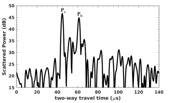
Thus, the received signal is composed by two echoes temporally separated by a two-way travel time ${\tau }_{ice}$(see Figure 1) and having intensities $P_s$ and $P_b$ given by:

$$\begin{array}{c}{P}_s=a_s{}^2{x}_0{}^2={\left({\rho }_s\frac{e^{-{\alpha }_{a}2H}}{H}{x}_0\right)}^2\\ P_b=a_b{}^2{x}_0{}^2={\left(\left(1-{\rho }_s{}^2\right){\rho }_b\frac{e^{-{\alpha }_{a}2H}}{H}{x}_0{e}^{-2{\alpha }_{ice}{\tau }_{icev}{v}_{ice}}\right)}^2\end{array},$$

(8)

where $x_0{}^2$ is the irradiated power.

As a final step, the ratio between basal and surface intensities is computed in order to remove from the inversion procedure the unknown quantities, that is, the ionospheric attenuation (${\alpha }_a)$ and the irradiated power ($x_0{}^2)$:

$$\frac{P_b}{P_s}={\left[\frac{(1-{{\rho }_s}^2){\rho }_b}{{\rho }_s}\right]}^2{e}^{-4{\alpha }_{ice}{\tau }_{ice}{v}_{ice}},$$

(9)

Equation (9) defines the forward electromagnetic model $d=g\left({\epsilon }_{ice}, {\epsilon }_b\right)$, which relates the measured quantities $d= P_b/P_s$ to the model parameters $({\epsilon }_{ice}, {\epsilon }_b)$ and will be used in the probabilistic inversion procedure to retrieve the basal permittivity.

4. Electromagnetic Properties of the SPLD Ice-Layer

The SPLD is predominantly composed by “dirty ice” that is a mixture of water ice with a variable volume fraction of dust [6,27]. For radar data interpretation, it is suitable to consider the microscopically complex mixture as macroscopically homogeneous and characterized by an effective dielectric permittivity. Several dielectric models have been proposed to estimate the permittivity of mixtures from the known dielectric properties and volume content of the phases [28]. In order to explore different scenarios for the composition of the SPLD, the dielectric permittivity of pure water ice and dirty ice (with different silicate dust volume fractions) is reported below in terms of real part of permittivity ε’ and attenuation factor α, estimated using the following formula: inversion procedure to retrieve the basal permittivity

$$\alpha =-\frac{\omega }{c}Im(\sqrt{\epsilon }),$$

(10)

where $\epsilon ={\epsilon }^{\prime }-i{\epsilon }^{″}$ is the complex relative permittivity.

4.1. Pure Water Iice

The dielectric properties of pure water ice have been intensively measured in laboratory over a wide range of temperatures and frequencies; however, the lack of a standard procedure in sample preparation and measuring methodology raises some questions about the reliability of the experimental data. Indeed, the dielectric measurements of pure water ice are affected by cooling procedure, aging, dislocation, cracks and fractures, gas bubbles and inclusions, chemical impurities, vacancies and other lattice imperfections [29,30]. Since literature data are heterogeneous in terms of temperature intervals and frequency ranges, the complex permittivity of pure water ice is here assumed according to the data provided by Kawada [31].

4.2. Dirty Ice

The real and imaginary part of the dielectric permittivity for dirty ice have been retrieved for four different values of silicate volume fraction (5,10, 15 and 20%) considering the medium as a two-phase mixture (ice/silicate). The Maxwell Garnett mixing rule [28] has been applied to determine the effective dielectric properties of the mixtures: the host medium is considered as pure water ice [31] and the inclusions are Martian meteorite dust ${\epsilon }_d=8.8\times \left(1-i 2\times {10}^{-3}\right)$ [32].

Figure 2. reports the attenuation at 4 MHz as a function of temperature for dust, pure water ice and dirty ice, evaluated at four different volume fractions (5, 10, 15 and 20%). The pure water ice shows a typical exponential decay with temperature, whereas no temperature dependence is exhibited by the dust. The behaviour of dirty ice is intermediate between the trends of water ice and dust.

Table 1. Real part of complex relative permittivity for different materials, constituents of SPLD.

	${\mathit{\epsilon }}^{\prime }$
Pure water ice	3.10
Dirty ice 5%	3.28
Dirty ice 10%	3.47
Dirty ice 15%	3.66
Dirty ice 20%	3.87

reports the values of the real part of the permittivity of the ice layer for the same conditions given in Figure 2. It is worth noting that the presence of the dust in the water ice also introduces a small variation in the real part of the dielectric permittivity (ranging from 3.1 to 3.9). These values (permittivity and attenuation) have been used in the inverse model to retrieve the basal material permittivity.

5. Probabilistic Approach for Basal Permittivity Estimation

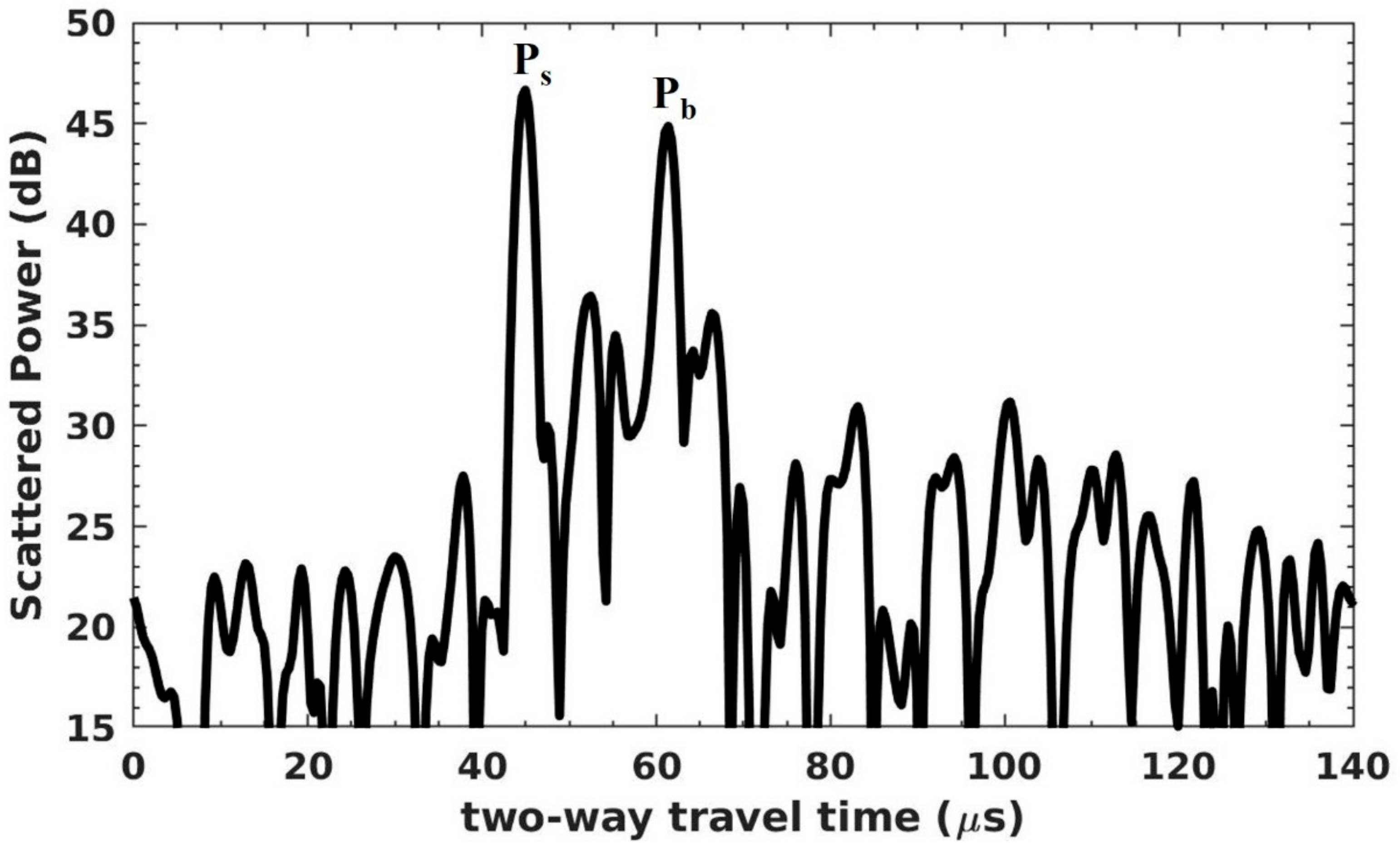
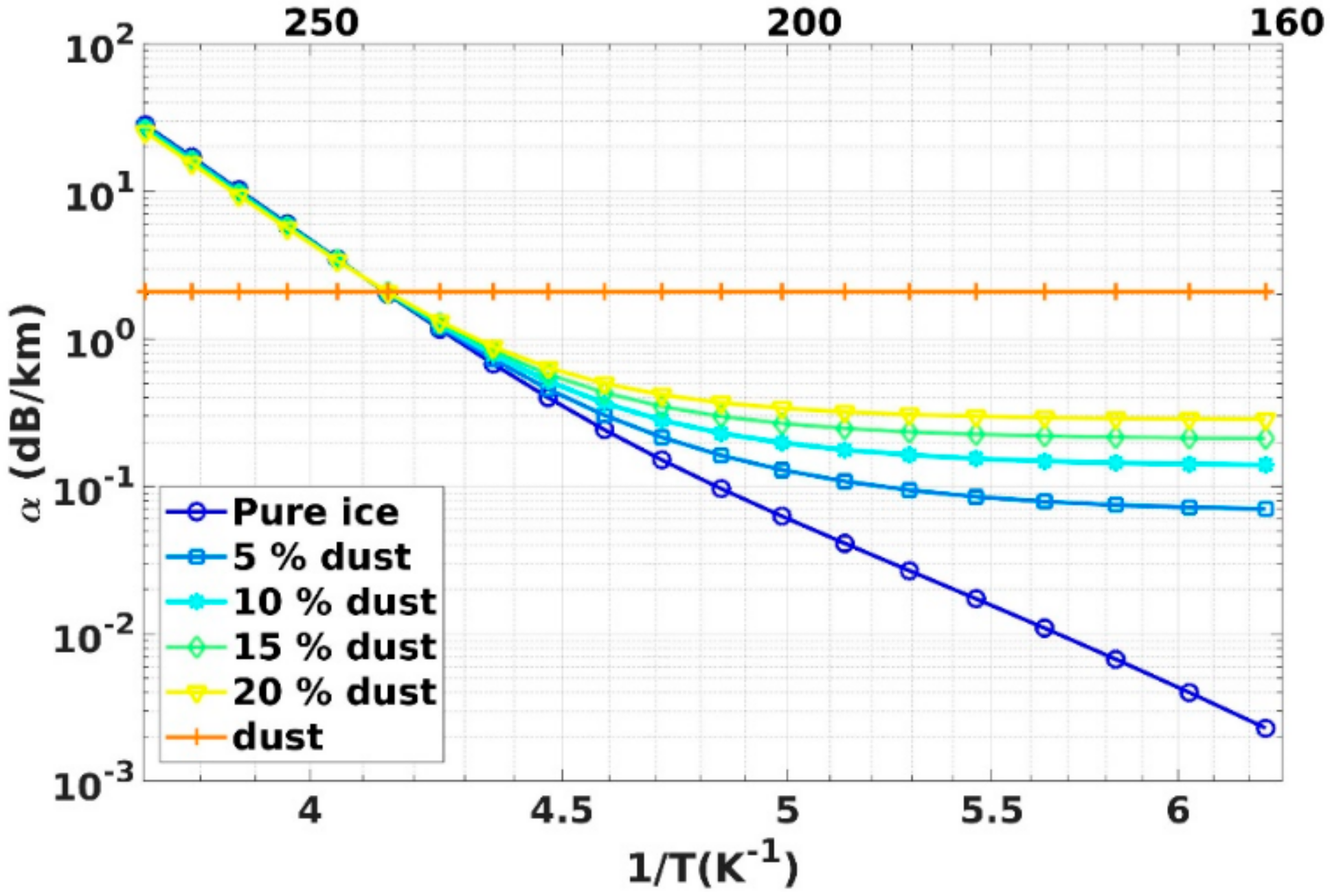
The permittivity ${\epsilon }_b$ is the physical quantity used to characterize the basal material underlying the SPLD and ultimately to detect the presence of liquid water. The inversion of equation (9) has been tackled by resorting to a probabilistic approach, where the solution of the inverse problem is stated as a combination of different states of information, that is, the probability density function (pdf) of the measured quantities (data) and the input (model parameters) [20]. To define the states of information on the input parameters $({\epsilon }_{ice}, {\epsilon }_b)$, few a-priori assumptions were done about the icy layer and the basal material. It is assumed for the ice-layer: (i) a composition made of a mixture of water ice and dust in variable proportions ($f_v\in \left[0.05,0.2\right]$); (ii) a linear temperature profile $T\left(z\right)$ with a fixed surface temperature ($T_s=160 K$) and a variable basal temperature ($T_b\in \left[170,270\right]K$); (iii) a complex permittivity computed using the procedure described in Section 4. The other input parameter is the basal permittivity value ${\epsilon }_b$, which is assumed to be a real quantity ranging from 3 to 1000. The quantities $T_b$ and $f_v$ have a remarkable effect on ${\epsilon }_{ice}$ and, consequently on the propagation parameters attenuation ${\alpha }_{ice}$ and velocity $v_{ice}$; this is shown in Figure 3 for the extremal values of the intervals $\left(f_v=0.05, T_b=170 K\right)$ and $(f_v=0.2, T_b=270 K)$.

In practice,$T_b$, $f_v$ and ${\epsilon }_b$ are the model parameters in the forward model (Equation (9)), therefore $d=g\left({\epsilon }_{ice},{\epsilon }_b\right)$ is rewritten as $d=g\left(m\right)$ where $m=\left(f_v{}^{*},T_b{}^{*},{\epsilon }_b{}^{*}\right)$ are the intrinsic model parameters. Because these quantities are always positive (Jeffrey parameters, see Tarantola [20]), the logarithmic of these parameters $w^{*}=\log \left(w/w_0\right)$ were used in the computation.

The inversion procedure consists of computing the posterior pdf, $\sigma \left(m\right)$, as the product of the data pdf $p_d\left(d\right)$ and the a-priori pdf on the model parameters $p_a\left(m\right),$ under the assumption that the model uncertainties are negligible with respect to the other uncertainties [20]:

$$\sigma \left(m\right)=\frac{1}{k}{p}_a\left(m\right)p_d\left(d\right){|}_{d=g\left(m\right)},$$

(11)

where $k={{\displaystyle \int }}_{-\infty }^{\infty }{p}_a\left(m\right)p_d\left(d\right){|}_{d=g\left(m\right)}dm$ is the normalization constant.

The marginal pdf, that is, the probability density function of the single model parameter, can be estimated integrating $\sigma \left(m\right)$ along the variables that have to be excluded in the final representation; for example, the posterior pdf of the basal permittivity $p_p\left({\epsilon }_b{}^{*}\right)$ is given by:

$$p_p\left({\epsilon }_b{}^{*}\right)={{\displaystyle \int }}_{-\infty }^{\infty }{{\displaystyle \int }}_{-\infty }^{\infty }\sigma \left(f_v{}^{*},T_b{}^{*},{\epsilon }_b{}^{*}\right)d{T}_b{}^{*}d{f}_v{}^{*},$$

(12)

Similar expressions hold for the posterior pdf $p_p\left(T_b{}^{*}\right)$ and $p_p\left(f_v{}^{*}\right)$.

6. Data Analysis and Results

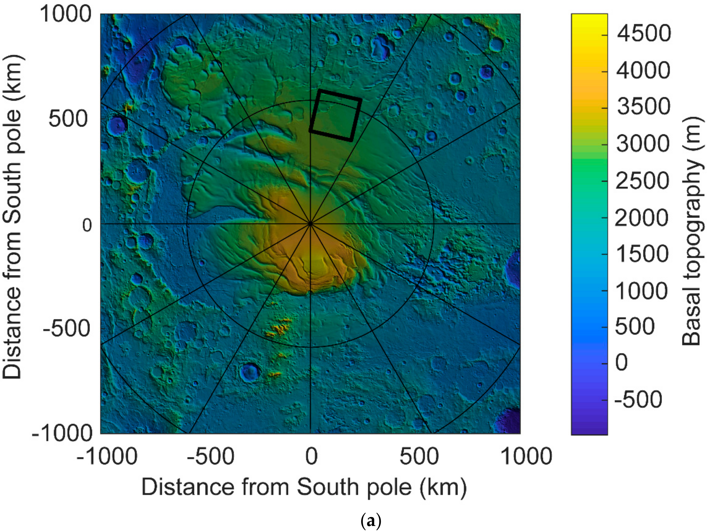
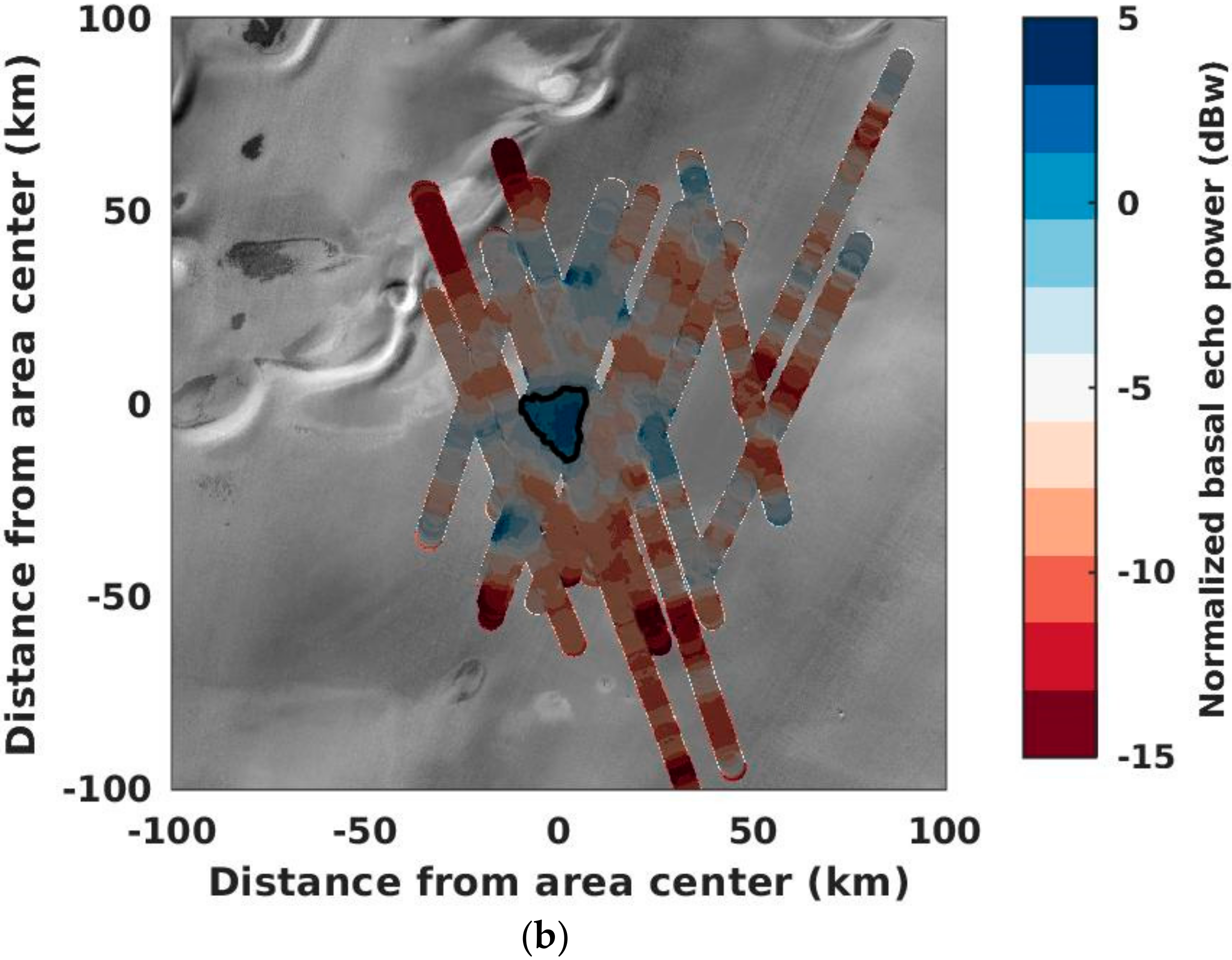
The probabilistic approach was applied to the data collected by MARSIS in a 200-km-wide area of Planum Australe, centred at 193°E, 81°S (Figure 4, panel a). In this area, a total of 24 radar profiles at 4 MHz were acquired using the onboard “Superframe” modality. The data at 3 and 5 MHz, are not presented in this work but they provide similar results to the ones at 4 MHz (cf. Orosei et al. [17]). In general, the data are characterized by the presence of two main echoes (see Figure 1), that are interpreted as the signal reflected by the surface and the base of SPLD, with a time delay of about $17 \mu s$ corresponding to an ice-thickness of about $1450 m$ assuming $v_{ice}=170 m/\mu s$. Figure 4, panel b depicts the spatial distribution of the power ratio $P_b/P_s$, that is, the basal echo power normalized to the median value of the surface echo power along each orbit; the black line defines a sub-area with high values of $P_b/P_s$, which is labelled “bright area.”

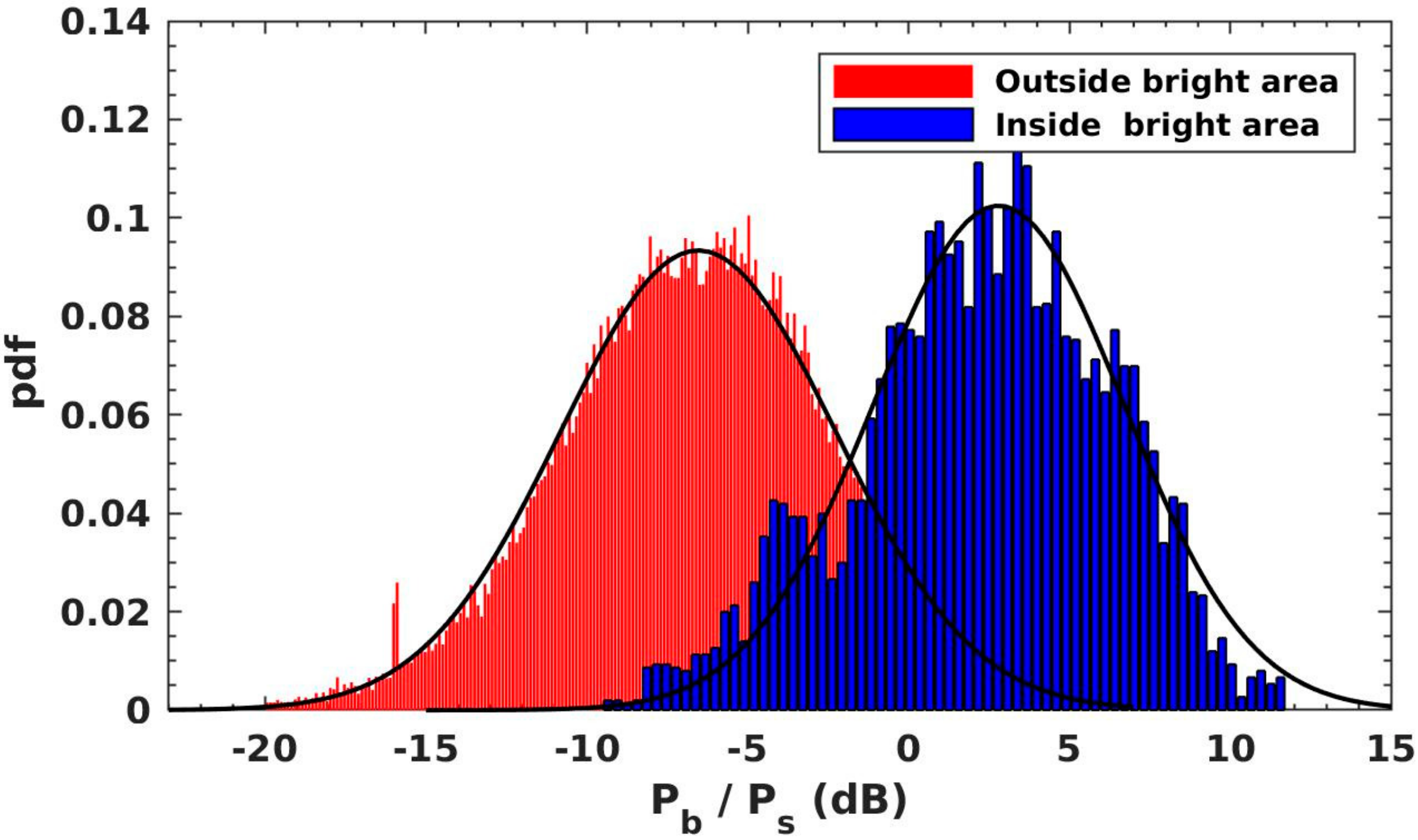
The distributions of $P_b/P_s$ inside and outside the bright area are shown in Figure 5; the best-fitting normal pdf (black line) is computed for both areas. The resulting mean and standard deviation values for the two distributions are (2.8, 3.9) dB (bright) and (−6.5, 4.3) dB (non-bright), respectively.

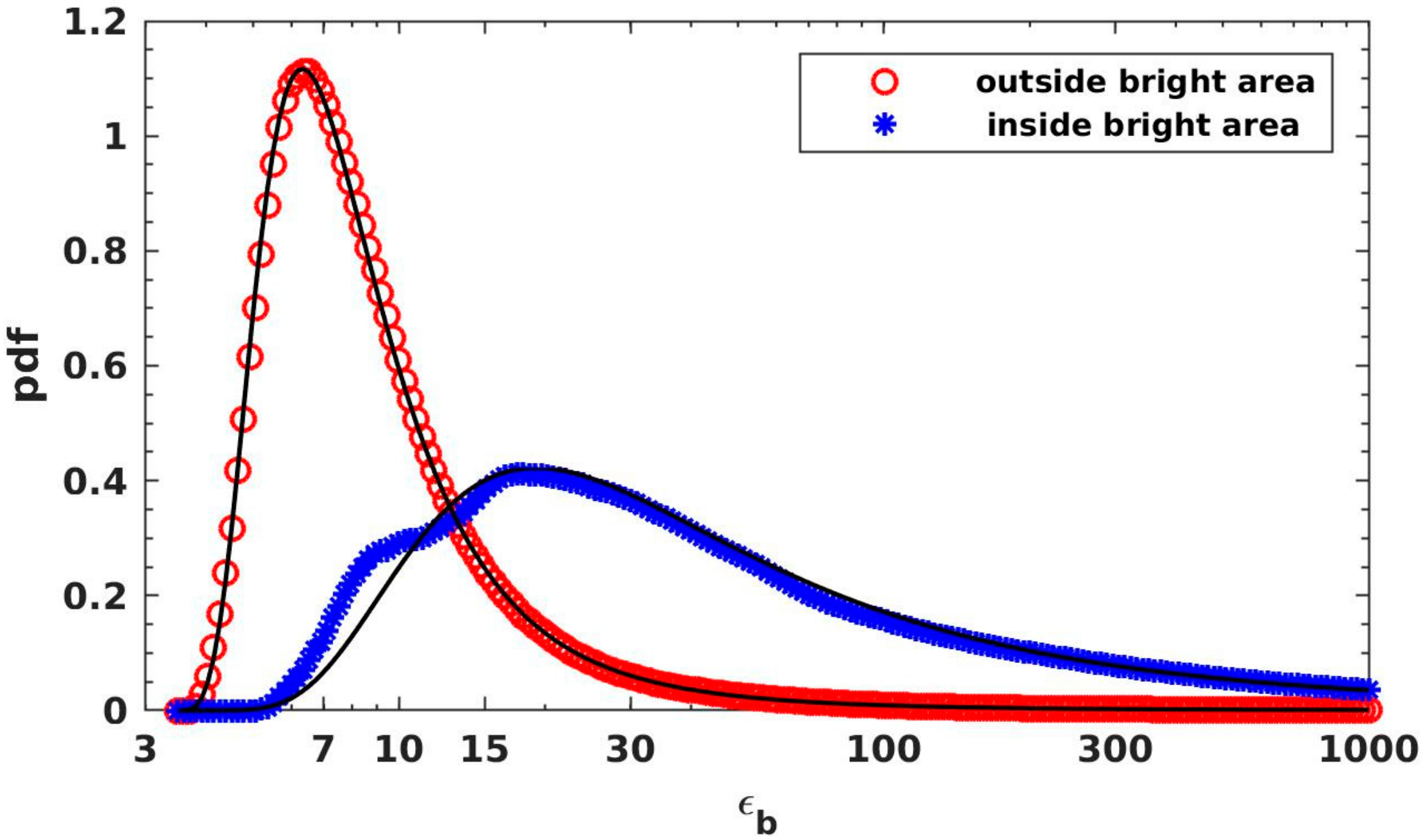
By applying the probabilistic approach discussed in Section 5, based on the forward electromagnetic modelling presented in Section 3, the posterior pdf of the basal permittivity $p_p\left({\epsilon }_b{}^{*}\right)$ inside and outside the bright area was obtained. The results achieved starting from the data distributions are represented with red and blue circles in Figure 6 whereas those obtained by using the curve fitting (Figure 5) are depicted by black lines. Note that the inversion procedure modifies the shape of the pdfs (increasing their skewness), as the relation between power ratio and basal permittivity is not linear (see Equation (9)). It follows that the $p_p\left({\epsilon }_b{}^{*}\right)$ is not symmetrical with a long tail on the side of the high basal permittivity values.

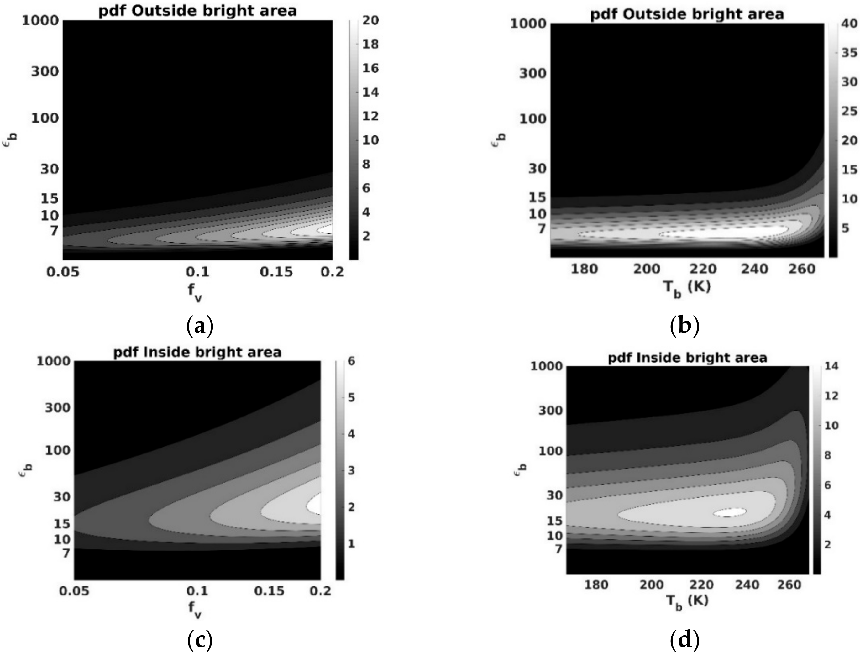
The effect of the temperature and volume fraction ($T_b, f_v$) on the basal permittivity estimation is shown in Figure 7, through the bidimensional posterior pdfs $p_p\left({\epsilon }_b{}^{*},T_b{}^{*} \right)$ and $p_p\left({\epsilon }_b{}^{*},f_v{}^{*} \right)$. The plots clearly indicate that outside the bright area (Figure 7a,b) the estimated value of ${\epsilon }_b$ is hardly sensitive to the volume fraction in the ice layer or to the basal temperature and it remains confined between about 4 and 15. Conversely, inside the bright area (Figure 7c,d), the estimated value of ${\epsilon }_b$ is much broader and ranges between about 10 and 100. Such a broadening increases with $T_b$ and $f_v$, due to the non-linearity of Equation (9) [19] and because of the remarkable effect of these two parameters on the signal attenuation (see Figure 3a).

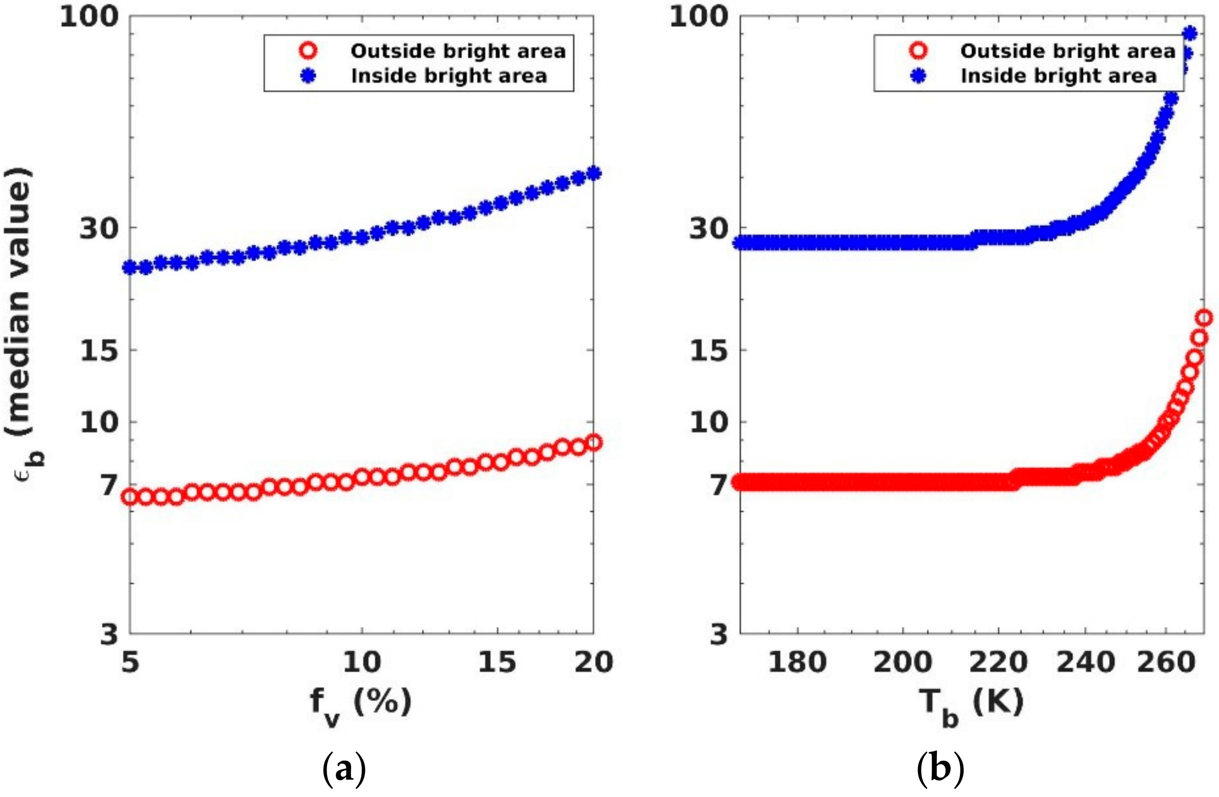
Finally, because in Orosei et al. [17] the median of the pdfs was used as statistical parameter to discriminate between dry and wet (liquid water) basal material conditions, Figure 8 reports the trend of the median values extracted from the posterior pdfs $p_p\left({\epsilon }_b,T_b\right)$ and $p_p\left({\epsilon }_b,f_v\right)$, as a function of $T_b$ and $f_v$. These results are consistent with those presented by Orosei et al. [17], as the basal permittivity outside the bright area has a median value around 7 and inside the bright area around 30. Figure 8 also shows that the basal permittivity is only slightly dependent on the ice-layer dust volume fraction and that the effect of the basal temperature is almost negligible up to the temperature $T_b=250K$. Above such a temperature, the basal permittivity attains higher values in both areas, but they still support the existence of two very distinct basal materials, one dry (non-bright) and one wet (bright).

7. Discussion

The achieved results indicate that up to a certain basal temperature (250 K), the thermal state of the icy layer does not appreciably affect the retrieved value of the basal permittivity. In other words, if the ice is cold the attenuation is negligible and the intensity of the reflected signal at the base of the icy layer is mostly due to the dielectric contrast between the ice and the basal material. Above such a temperature, the attenuation becomes appreciable and the estimated value of the basal permittivity strongly increases; this effect, however, does not change the outcome of the analysis regarding the state of the two areas (dry and wet). Moreover, our results also indicate that the percentage of the dust volume fraction in the icy layer weakly but steadily increases the value of the estimated basal permittivity, because the dust content affects both the attenuation in the icy material and the basal dielectric contrast.

It should be noted that the results have been obtained assuming in the model an abrupt dielectric interface between air and solid ice. Conversely, considering a gradual change in permittivity, that is, for example the presence of a transition layer where the material density increases with depth, the surface echo intensity would be smaller. In the extreme case where the thickness of the transition zone was exactly a quarter wavelength, this would create a perfect matching layer that would completely suppress the reflected echo. Thus, the gradual variation in surface permittivity could produce strong $P_b/P_s$ values also in case of basal dry material. This fact has been already discussed in Orosei et al. [17], by considering at the top of the SPLD the presence of a CO₂ ice layer having a permittivity value ranging between that of air and water ice [30]. This scenario was excluded, first of all because of the very specific and unlikely physical conditions required (perfect matching layer at three different frequencies, 3, 4 and 5 MHz) and secondly, because for different layer thicknesses (non-resonant layer) they do not cause sufficiently strong basal reflections. Alternatively, it could be possible to assume on the top of the SPLD the existence of a layer of snow/firn similar to that present on the terrestrial polar ice sheets, which would reduce surface reflectivity. Again, this hypothesis can be discarded because, on Mars, the total humidity of the Martian atmosphere can produce at best a layer of snow having a thickness of 20 micron that is not sufficient to affect the radar response. To our knowledge, no other material detected or hypnotized to be present on the Martian polar caps surface could generate a transition layer capable to depress the surface echo and thus enhance the basal to surface echo intensity ratio.

8. Conclusions

The search for liquid water in the Martian subsurface using a radar sounder on-board a spacecraft is particularly challenging, due to the lack of information regarding the physical properties of the crust and the surrounding environment. In these conditions, the only viable way to properly retrieve the permittivity of the material underlying the icy layer and detect the presence of liquid water, is adopting a robust inversion procedure. In this work, it has been shown that, making some realistic assumptions regarding the physical properties of surface and subsurface material and using the subsurface to surface power ratio, it is possible to apply a probabilistic inversion approach that allows to unequivocally discriminate between dry and wet basal areas. The proposed method is particularly effective to properly account for the effect of the uncertainties associated to the physical parameters and the measured data in the non-linear inversion procedure.

The proposed approach can be applied for the estimation of the subsurface material dielectric properties using data acquired by a radar sounder on-board remote platforms on Earth and beyond. In particular, it could be a valuable tool for the detection of subsurface liquid water in the Jovian icy moons, where the thermal state of the icy crusts and the presence of salty and acid impurities could strongly affect the electromagnetic wave propagation.