Response to Variations in River Flowrate by a Spaceborne GNSS-R River Width Estimator


1
SRI International, Ann Arbor, MI 48105, USA
2
Climate and Space Dept, University of Michigan, Ann Arbor, MI 48109, USA
*
Author to whom correspondence should be addressed.
Remote Sens. 2019, 11(20), 2450; https://0-doi-org.brum.beds.ac.uk/10.3390/rs11202450
Submission received: 27 September 2019
/
Revised: 16 October 2019
/
Accepted: 18 October 2019
/
Published: 22 October 2019
(This article belongs to the Special Issue GPS/GNSS for Earth Science and Applications)
Abstract
:In recent years, the use of Global Navigation Satellite System-Reflectometry (GNSS-R) for remote sensing of the Earth’s surface has gained momentum as a means to exploit existing spaceborne microwave navigation systems for science-related applications. Here, we explore the potential for using measurements made by a spaceborne GNSS-R bistatic radar system (CYGNSS) during river overpasses to estimate its width, and to use that width as a proxy for river flowrate. We present a case study utilizing CYGNSS data collected in the spring of 2019 during multiple overpasses of the Pascagoula River in southern Mississippi over a range of flowrates. Our results demonstrate that a measure of river width derived from CYGNSS is highly correlated with the observed flowrates. We show that an approximately monotonic relationship exists between river flowrate and a measure of river width which we define as the associated GNSS-R width (AGW). These results suggest the potential for GNSS-R systems to be utilized as a means to estimate river flowrates and widths from space.
1. Introduction
Knowledge of river streamflow is crucial for a number of water-related applications. For example, streamflow information is needed for hydrological modeling, watershed management, flood monitoring and warning systems, and hydrodynamic power management. Despite the need for streamflow data, existing in situ streamflow gauge networks are limited in number, particularly in remote regions, and are on the decline worldwide [1]. A number of remote-sensing-based algorithms for estimating streamflow have been proposed [2,3]; however, these algorithms require ancillary data and/or a priori knowledge of the river properties that precludes their use on a global scale. Furthermore, in order to be useful for short-term flood monitoring during extreme conditions, the algorithms require up-to-date remote sensing measurements at high spatial resolution that traditional satellite systems cannot provide. Existing Global Navigation Satellite System-Reflectometry (GNSS-R) systems present the potential for exploiting high-temporal-resolution data over large scales for use as inputs to flowrate algorithms, or as a means of developing a novel remote sensing signature for river properties (e.g., width) that correlate directly to streamflow. To investigate this potential, we used bistatic radar data from the NASA Cyclone Global Navigation Satellite System (CYGNSS) Mission to study the signal response to a range of flowrates over a segment of an uncontrolled river. Due to the high sensitivity of the CYGNSS signal to land/water boundaries, water bodies on the order of 100 m or less in width have been observed to create a well-defined signal response [4]. Our results indicate that the signal waveform width corresponding to the river is sensitive to flowrate due to the changing width with increased flows. We introduce the concept of an associated GNSS-R width (AGW) that maps approximately linearly to observed river streamflow. Our results indicate that the river’s AGW is highly correlated with changes in its streamflow at high flowrates and stream heights (when the river can be expected to overspill its banks).
2. Materials and Methods
2.1. CYGNSS Background
The CYGNSS mission is a Global Navigation Satellite Systems-Reflectometry (GNSS-R) bistatic radar system that was launched on 15 December 2016 and consists of eight microsatellites, each with a four-channel Global Positioning System (GPS) L1 coarse acquisition (C/A) radar receiver. The main goal of the CYGNSS mission is rapid sampling of ocean surface winds in the inner core of tropical cyclones. However, several qualities unique to CYGNSS make its observations highly useful for overland applications as well. Namely, the measurement modality, near-specular bistatic radar using GPS transmissions provides the ability to see through heavy rain and vegetation. The small satellite constellation architecture supports high revisit rates over a large portion of the globe (+/−38 degrees latitude), allowing for frequent updates and tracking of extreme weather events. Initial studies have demonstrated CYGNSS’s high sensitivity to land/water boundaries and its ability to delineate river systems with a high degree of detail [4].
2.2. Theoretical Basis of the High-Spatial-Resolution Land/Water Mapping Capability
Measurement of small inland water bodies with CYGNSS is possible due to the high-spatial-resolution capability of bistatic radar over coherent scattering scenes with low roughness (i.e., inland water bodies), which allows for delineation of water bodies that are much smaller than the nominal footprint of the data. The signal strength received by a GNSS-R bistatic radar from a rough, incoherently scattering surface is given by [5] as
and the signal strength received from a smooth, coherently scattering surface filling the first Fresnel zone is given by
where:
- (τ, f) = delay and Doppler coordinates in the delay Doppler map (DDM)
- PT = transmitted power
- GR = receive antenna gain
- GT = transmit antenna gain
- Λ = lag correlation function due to the correlation with a local replica of the GPS pseudorandom noise (PRN) code
- S = Doppler filter response due to selective filtering of the Doppler-shifted received signal
- = vector distances from the specular point to the transmitter and receiver, respectively
- σ0 = normalized scattering cross section of the rough surface (BRCS)
- λ = signal wavelength (19 cm)
- = vector distance from a point on the Earth’s surface to the specular point
- Zf = term to account for area/shape of smooth surface region affecting first Fresnel zone
- = surface Fresnel reflectivity for incidence angle
- ; electromagnetic wavenumber
- h = surface rms height
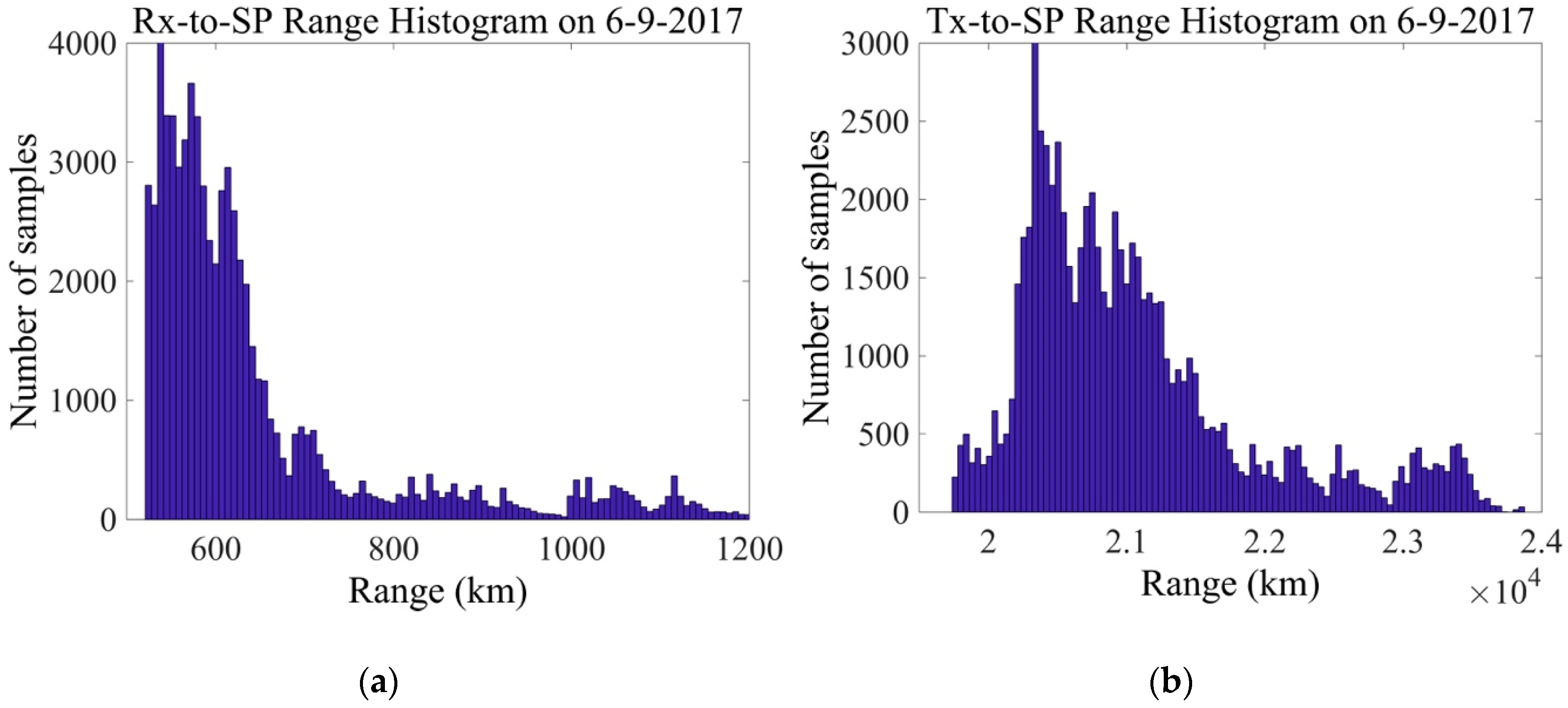
For heterogeneous conditions containing both smooth and rough surfaces within the region bounded by the lag correlation and Doppler filter responses, the net received signal strength is an area-weighted composite of the two contributions. The relative strengths of the two components are largely determined by their differing dependencies on the propagation distances, and , in Equations (1) and (2). The two distances vary from sample to sample, depending on the measurement geometry of the GPS transmitter, the specular point, and the GNSS-R bistatic radar receiver. The variation of the two distances for CYGNSS throughout a typical 24-hour period is shown in Figure 1, where it can be seen that , the distance from specular point to the receiver, varies between ~500 and 1200 km, and , the distance from GPS transmitter to specular point, varies between ~19,500 and 24,000 km.
Using Equations (1) and (2), we can compute a first-order approximation of the relative strength of signals received from coherent and incoherent portions of a heterogeneous scene as
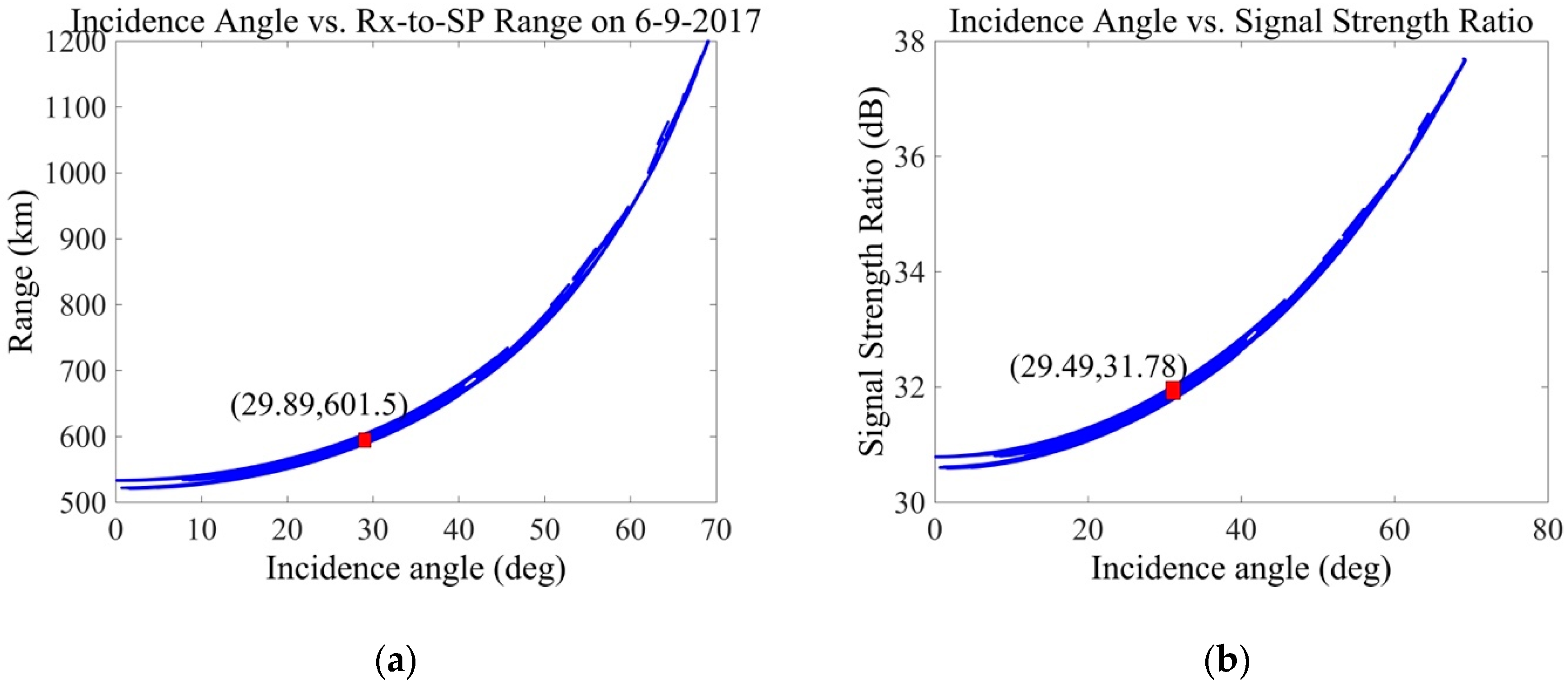
where Ainc is the scattering area of the incoherent region bounded by the lag correlation and Doppler filter response functions. For the GPS L1 C/A signal used by CYGNSS, Ainc is ~ 15 × 15 km2. Variations in both and are well parameterized by the incidence angle of the propagating signal at the specular reflection point. This is illustrated in Figure 2a,b, which respectively plot the incidence angle vs. and vs. the relative signal strength between coherent and incoherent scatterers for the same 24-h collection of data. The greatest number of samples occurs near an incidence angle of ~30° and = 600 km. An incidence angle of ~30° corresponds to the angle of maximum gain in the receive antenna pattern.
The strength of the received signal scattered from coherent (smooth) surface features is more than 1000-times stronger than that received from incoherent (rough) surfaces at all measurement geometries, with a value of 1,600 (32 dB) at the most common incidence angle. This enhanced sensitivity explains why small, smooth water bodies occupying a very small fraction of the total incoherent scattering area can make such a dominant contribution to the net received signal. It also explains why very small inland water bodies can be so finely resolved by the GNSS-R bistatic radar measurements. For example, a small inland water body that fills only 1% of the first Fresnel zone (-20 dB beam filling) would still produce an 11–17 dB higher contribution to the total received signal strength than would the surrounding incoherently scattered signal from rough land surfaces.
2.3. Case Study: Pascagoula River
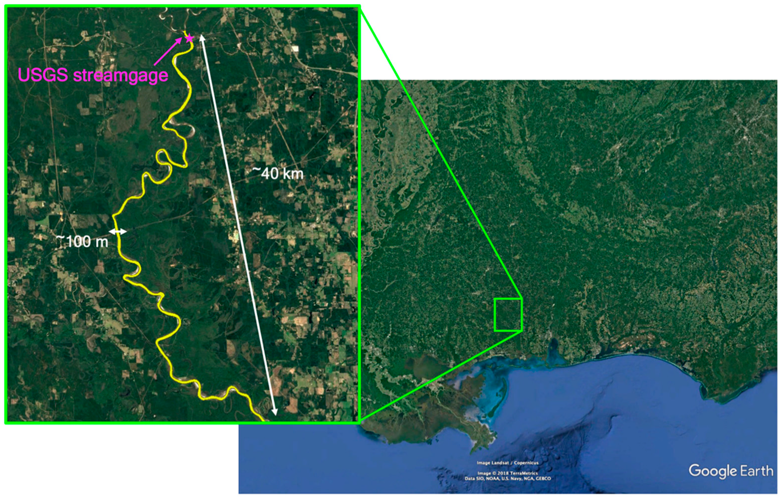
A case study examining the relationship between the river signal width estimated from CYGNSS measurements and river flowrate was carried out using data from five CYGNSS overpasses of a section of the Pascagoula River in southern Mississippi (Figure 3) collected in April 2019. The Pascagoula River was chosen for the case study because of its highly dynamic nature and the availability of streamflow data from a USGS streamflow gauge located at the head of the river.
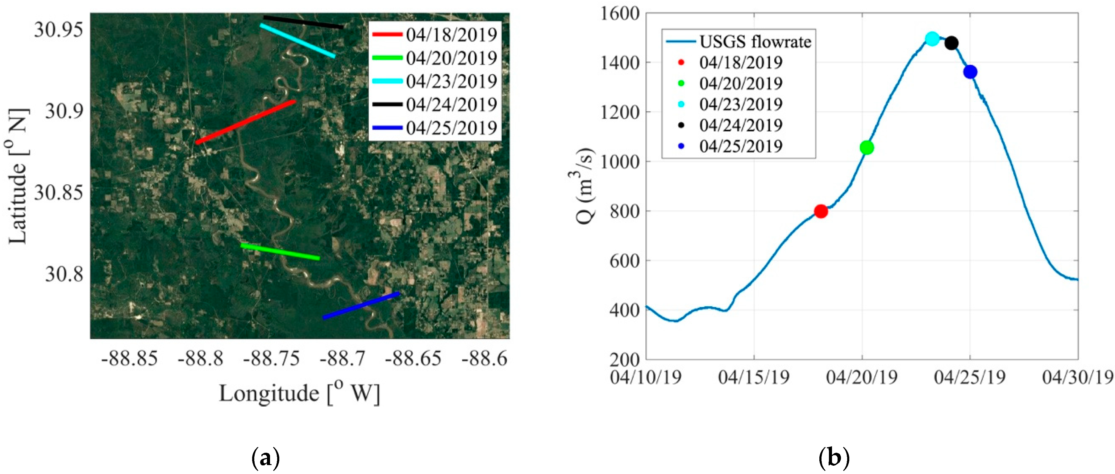
The standard Level 1 CYGNSS data products are averaged onboard over 1 second increments (equivalent to ~7 km of forward motion), which precludes their use for measuring small water bodies. Hence, we implemented special collections of the raw intermediate frequency (IF) data over 1 second intervals for this study. The raw IF data were post-processed using an incoherent averaging period of 50 ms. The data were collected over the period 18–25 April 2019 over a latitude range of ~30.78°–30.94° N. The track locations and the contemporaneous flowrates as measured by USGS gauge 02479000 are shown in Figure 4a,b, respectively. According to the North American River Width data set (NARWidth), a database that provides width measurements based on Landsat imagery corresponding to mean streamflow for rivers in North America greater than 30 m wide [6], the average width along this section of the river under mean flow conditions is 94 m, with a standard deviation of 33 m. The observed flowrates contemporaneous with the raw IF data collections over the river correspond to measured gauge heights ranging from ~6–7 m, with the three highest flowrates exceeding the National Weather Service’s flood stage limit of 6.7 m at the gauge location. At these heights, the river should be expanding in width along its banks.
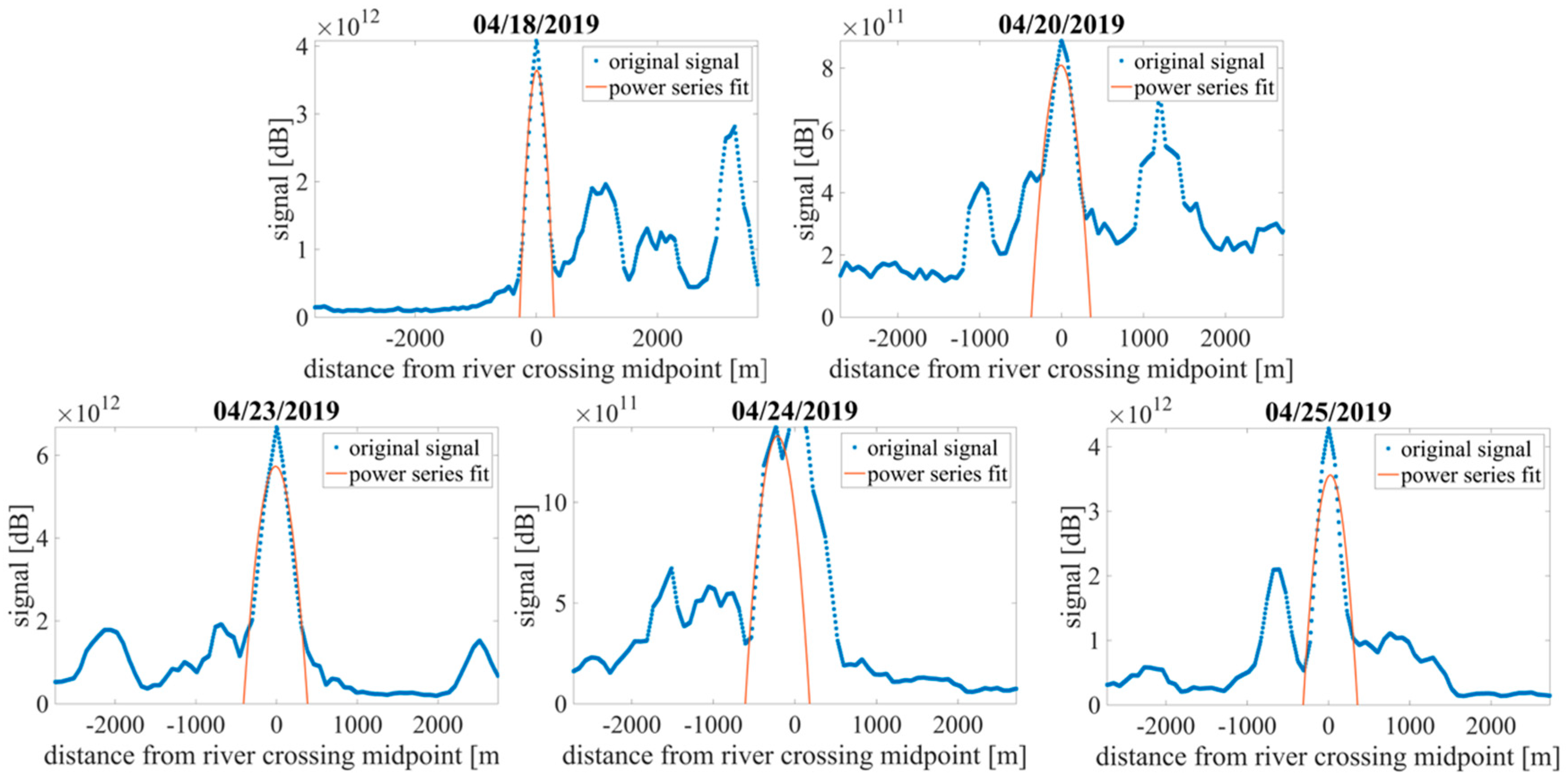
For each river overpass, the river width associated with the CYGNSS signal is estimated by fitting a second-order power series to the portion of the waveform corresponding to the river body. The resulting fitted curves are extrapolated to a signal strength of zero before and after the signal peak centered on the river, and the associated width is defined as the distance between the two zero-crossings. This method is illustrated by a number of examples in Figure 5. One complication with this approach is that the CYGNSS signal is very sensitive to nearby waterbodies within a roughly 600 m radius of the specular point on the ground (the first Fresnel zone). Because the Pascagoula is surrounded by many U-shaped (oxbow) lakes, formed by meandering sections of river, the portion of the signal used for the power series fit needs to be limited to exclude the influence of these surrounding water bodies on the waveform corresponding to the river itself. However, using too little of the waveform makes it difficult to discern the true signal width. We find that fitting the power series to the portion of the signal within ~20% of its peak at river center produces the best correlation between the resulting river width and flowrate. This 20% value emphasizes the portion of the waveform nearest the center of the river crossing and least affected by other waterbodies or other sources of clutter nearby the river. The estimated width is then scaled by the cosine of the angle of the CYGNSS track relative to a line perpendicular to the river’s banks; this is necessary to estimate the width of the river from bank to bank, instead of the along track distance of the CYGNSS observation. We refer to the final width determined in this way as the associated GNSS-R width, or AGW, of the river.
3. Results
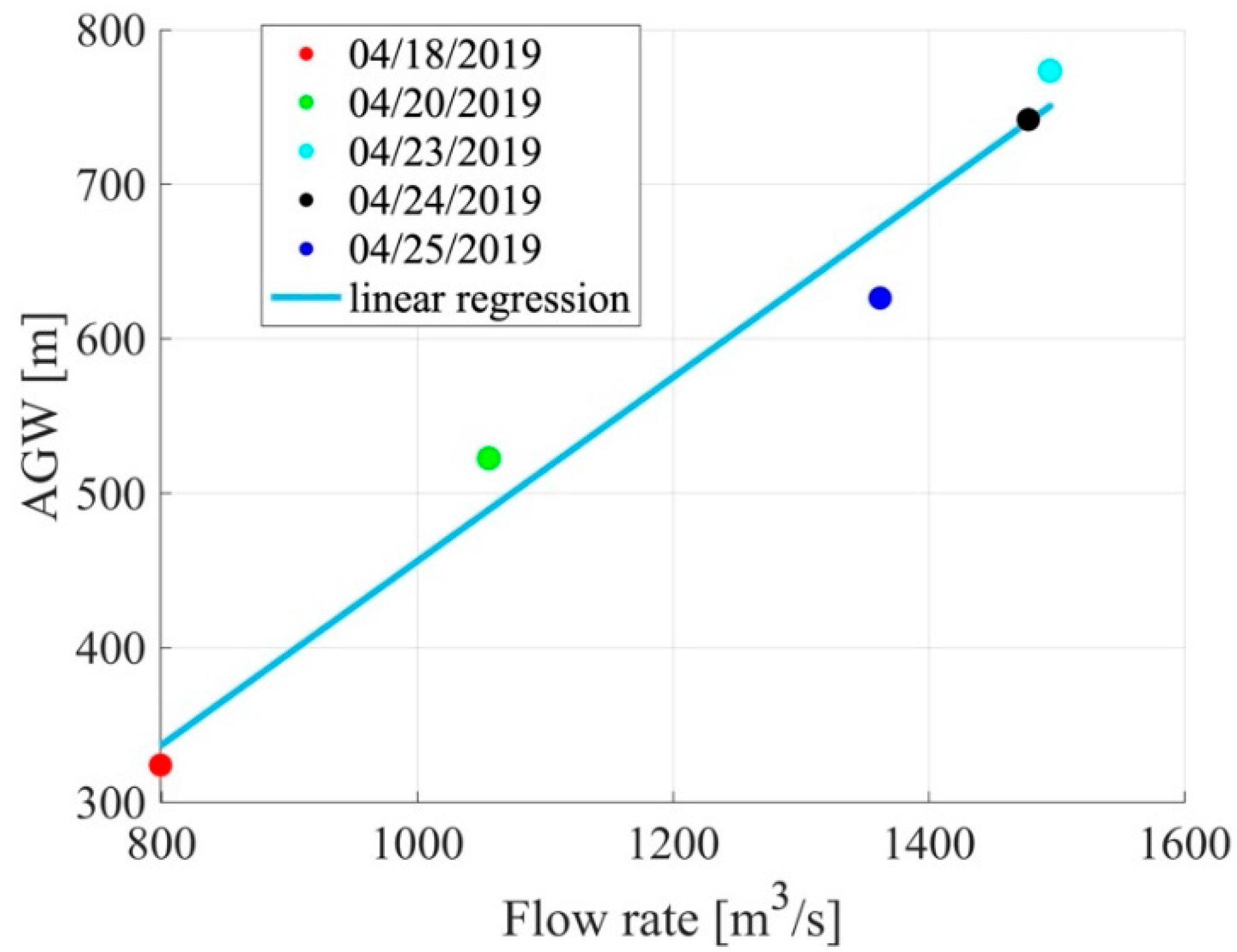
The fitted power series for each of the overpasses is shown in Figure 5, where the observed signal at each time step for each track is plotted in blue, and the red line shows the power series fitted to the signal within 22% of the peak at river center. Figure 6 shows the results of the linear regression between the AGW and the observed Pascagoula flowrates. The R2 coefficient of the regression is 0.97.
4. Discussion
The monotonic relationship between the AGW and the flowrates for the Pascagoula River case study shown in Figure 6 indicates the presence of a signal that can be exploited for remote-sensing-based river flowrate algorithms. However, further research is required to determine the robustness and limits of this relationship. One important factor is the lack of exact repeat overpass locations by CYGNSS due to the asynchronous relationship between its orbit properties and those of the GPS satellites. Since there are natural variations in width along the river on the order of tens of meters, some of the decorrelation between AWG and flowrate in Figure 6 may be a result of natural variations in width along the river that have not been accounted for in our analysis. It also remains to be determined over what range of flowrates the AGW metric correlates with the river streamflow. We hypothesize that at flowrates that correspond to stage heights much lower than the flood stage height for the river, the AGW may cease to show as strong a correlation to flowrate due to the river being contained within its banks. At low enough flows, however, sand bars will become exposed and the AGW may again correlate strongly with the flowrate. These limits to the algorithm will be explored in future studies with the additional collection of raw IF data over the Pascagoula River and other rivers.
The potential utility of the AGW metric is vast; many remote-sensing-based flowrate estimation algorithms require knowledge of river width, which could be derived from the AGW. The river width estimations could provide up-to-date input to remote-sensing-based flowrate retrieval algorithms such as the at-many-stations hydraulic geometry (AMHG) method [7,8,9], the mean-annual flow and geomorphology (MFG), and mean flow with constant roughness (MFCR) streamflow estimation algorithms, and others that have been proposed in recent years (e.g., [10,11]). Moreover, our results suggest that it may be possible to derive a direct relationship between the flowrate and AGW, bypassing the need for a complicated flowrate estimation algorithm entirely. It should be noted that the question of whether or how best one could expand this method to river width estimation on a global scale is unclear. The correlation between flowrate and AGW demonstrated on the Pascagoula River needs to be tested elsewhere. The relationship between the two may vary, for example, with river bathymetry or the flowrate itself. A comprehensive investigation would likely require ancillary information about both.
5. Conclusions
Analysis of a spaceborne GNSS-R-based signal response to varying flowrates over a section of the Pascagoula River has been conducted using data from a series of raw IF river overpasses during the period 18–25 April 2019. The width of the signal corresponding to the river overpasses was deduced by fitting a power series to a portion of the waveform bounded by limits of ~20% of the peak signal at river center to either side of the peak. The signal width, referred to as the river’s associated GNSS-R width (AGW), is then adjusted for the track angle of the satellite’s specular point relative to a perpendicular line across the banks. The river AGW maps approximately monotonically and linearly to the observed flowrates contemporaneous with the data collections. While this finding indicates high potential for exploiting GNSS-R based signals for measuring river streamflow directly or as an input to remote-sensing-based flowrate retrieval algorithms, further work with more extensive datasets will be necessary to determine the robustness of the method and the limits on its applicable flowrate ranges.
Author Contributions
Conceptualization, C.R. and A.W.; Methodology, C.R. and A.W.; Software, C.R and A.W.; Validation, C.R. and A.W.; Formal analysis, C.R. and A.W.; Investigation, C.R. and A.W.; Resources, C.R. and A.W.; Data curation, A.W.; Writing—original draft preparation, C.W. and A.W.; Writing—review and editing, C.R. and A.W.; Visualization, C.R. and A.W.; Supervision, C.R. and A.W.; Project administration, C.R. and A.W.; Funding acquisition, C.R. and A.W.
Funding
This research was funded by NASA Earth Science Research Program, Grant/Cooperative Agreement Number 80NSSC18K0702 with SRI and NASA Science Mission Directorate contract NNL13AQ00C with U-M.
Acknowledgments
The authors would like to thank the NASA CYGNSS Science Team for facilitating the collection and processing of the raw IF data used in this research.
Conflicts of Interest
The authors declare no conflict of interest.
References
- Shiklomanov, A.I.; Lammers, R.B.; Vörösmarty, C.J. Widespread decline in hydrological monitoring threatens pan-Arctic research. Eos Trans. Am. Geophys. Union 2002, 83, 13–17. [Google Scholar] [CrossRef]
- Durand, M.; Gleason, C.; Garambois, P.-A.; Bjerklie, D.; Smith, L.; Roux, H.; Rodriguez, E.; Bates, P.D.; Pavelsky, T.M.; Monnier, J. An intercomparison of remote sensing river discharge estimation algorithms from measurements of river height, width, and slope. Water Resour. Res. 2016, 52, 4527–4549. [Google Scholar] [CrossRef] [Green Version]
- Sichangi, A.W.; Wang, L.; Yang, K.; Chen, D.; Wang, Z.; Li, X.; Zhou, J.; Liu, W.; Kuria, D. Estimating continental river basin discharges using multiple remote sensing data sets. Remote. Sens. Environ. 2016, 179, 36–53. [Google Scholar] [CrossRef] [Green Version]
- Ruf, C.S.; Chew, C.; Lang, T.; Morris, M.G.; Nave, K.; Ridley, A.; Balasubramaniam, R. A new paradigm in earth environmental monitoring with the CYGNSS small satellite constellation. Sci. Rep. 2018, 8, 8782. [Google Scholar] [CrossRef] [PubMed]
- Balakhder, A.; Al-Khaldi, M.; Johnson, J. On the coherency of ocean and land surface specular scattering for GNSS-R and signals of opportunity systems. IEEE Trans. Geosci. Remote Sens. 2019, 57, 1–11. [Google Scholar] [CrossRef]
- Allen, G.H.; Pavelsky, T.M. Patterns of river width and surface area revealed by the satellite-derived North American river width data set. Geophys. Res. Lett. 2015, 42, 395–402. [Google Scholar] [CrossRef]
- Gleason, C.J.; Smith, L.C. Toward global mapping of river discharge using satellite images and at-many-stations hydraulic geometry. Proc. Natl. Acad. Sci. USA 2014, 111, 4788–4791. [Google Scholar] [CrossRef] [PubMed] [Green Version]
- Gleason, C.J.; Smith, L.C.; Lee, J. Retrieval of river discharge solely from satellite imagery and at-many-stations hydraulic geometry: Sensitivity to river form and optimization parameters. Water Resour. Res. 2014, 50, 9604–9619. [Google Scholar] [CrossRef]
- Pavelsky, T.M. Using width-based rating curves from spatially discontinuous satellite imagery to monitor river discharge. Hydrol. Process. 2014, 28, 3035–3040. [Google Scholar] [CrossRef]
- Bjerklie, D.M.; Moller, D.; Smith, L.C.; Dingman, S.L. Estimating discharge in rivers using remotely sensed hydraulic information. J. Hydrol. 2005, 309, 191–209. [Google Scholar] [CrossRef]
- Yoon, Y.; Durand, M.; Merry, C.J.; Clark, E.A.; Andreadis, K.M.; Alsdorf, D.E. Estimating river bathymetry from data assimilation of synthetic SWOT measurements. J. Hydrol. 2012, 464–465, 363–375. [Google Scholar] [CrossRef]
Figure 1.
Histogram of propagation distances: (a) (from specular point to CYGNSS receiver); (b) (from GPS transmitter to specular point) for a full day of samples on 9 June 2017.
Figure 1.
Histogram of propagation distances: (a) (from specular point to CYGNSS receiver); (b) (from GPS transmitter to specular point) for a full day of samples on 9 June 2017.

Figure 2.
Dependence on incidence angle of: (a) propagation distances from specular point to receiver; (b) relative signal strength received from coherent and incoherent scenes for one full day of samples on 9 June 2017. The red dots indicate the incidence angles at which the greatest number of samples occurs.

Figure 3.
Google Earth imagery of southern Pascagoula River in Mississippi. The location of the USGS streamflow gauge (USGS 02479000) is shown at the head of the river. The mean width along the roughly 40 km span of the river where collections took place is ~100 m.
Figure 3.
Google Earth imagery of southern Pascagoula River in Mississippi. The location of the USGS streamflow gauge (USGS 02479000) is shown at the head of the river. The mean width along the roughly 40 km span of the river where collections took place is ~100 m.

Figure 4.
April 2019 raw IF data collections over the Pascagoula River: (a) track locations; (b) corresponding flowrates at the time of each overpass (color coded to match the track locations plotted on the left), plotted over the USGS flowrates over the time period spanning the data collections.
Figure 4.
April 2019 raw IF data collections over the Pascagoula River: (a) track locations; (b) corresponding flowrates at the time of each overpass (color coded to match the track locations plotted on the left), plotted over the USGS flowrates over the time period spanning the data collections.

Figure 5.
Fitted power series for each of the five April 2019 Pascagoula overpasses, using a threshold of 22% of the peak as the cutoff for the portion of the waveform to be fitted.
Figure 5.
Fitted power series for each of the five April 2019 Pascagoula overpasses, using a threshold of 22% of the peak as the cutoff for the portion of the waveform to be fitted.

Figure 6.
Linear regression between the river AGW derived from CYGNSS observations and the river flow rate measured by the USGS stream gauge. The R2 coefficient is 0.97. Marker colors correspond to the tracks and flowrates shown in Figure 4.
Figure 6.
Linear regression between the river AGW derived from CYGNSS observations and the river flow rate measured by the USGS stream gauge. The R2 coefficient is 0.97. Marker colors correspond to the tracks and flowrates shown in Figure 4.

© 2019 by the authors. Licensee MDPI, Basel, Switzerland. This article is an open access article distributed under the terms and conditions of the Creative Commons Attribution (CC BY) license (http://creativecommons.org/licenses/by/4.0/).
Share and Cite
MDPI and ACS Style
Warnock, A.; Ruf, C. Response to Variations in River Flowrate by a Spaceborne GNSS-R River Width Estimator. Remote Sens. 2019, 11, 2450. https://0-doi-org.brum.beds.ac.uk/10.3390/rs11202450
AMA Style
Warnock A, Ruf C. Response to Variations in River Flowrate by a Spaceborne GNSS-R River Width Estimator. Remote Sensing. 2019; 11(20):2450. https://0-doi-org.brum.beds.ac.uk/10.3390/rs11202450
Chicago/Turabian StyleWarnock, April, and Christopher Ruf. 2019. "Response to Variations in River Flowrate by a Spaceborne GNSS-R River Width Estimator" Remote Sensing 11, no. 20: 2450. https://0-doi-org.brum.beds.ac.uk/10.3390/rs11202450
Note that from the first issue of 2016, this journal uses article numbers instead of page numbers. See further details here.