Combining Machine Learning and Compact Polarimetry for Estimating Soil Moisture from C-Band SAR Data


1
CNR-IFAC, via Madonna del Piano, 10–50019 Firenze, Italy
2
Science and Technology Branch, Environment and Climate Change Canada, Government of Canada, Dorval, QC H9P 1J3, Canada
*
Author to whom correspondence should be addressed.
Remote Sens. 2019, 11(20), 2451; https://0-doi-org.brum.beds.ac.uk/10.3390/rs11202451
Submission received: 27 September 2019
/
Revised: 15 October 2019
/
Accepted: 17 October 2019
/
Published: 22 October 2019
(This article belongs to the Special Issue Compact Polarimetric SAR)
Abstract
:This research aimed at exploiting the joint use of machine learning and polarimetry for improving the retrieval of surface soil moisture content (SMC) from synthetic aperture radar (SAR) acquisitions at C-band. The study was conducted on two agricultural areas in Canada, for which a series of RADARSAT-2 (RS2) images were available along with direct measurements of SMC from in situ stations. The analysis confirmed the sensitivity of RS2 backscattering (σ°) to SMC. The comparison of SMC with the compact polarimetry (CP) parameters, computed from the RS2 acquisitions by the CP data simulator, pointed out that some CP parameters had a sensitivity to SMC equal or better than σ°, with correlation coefficients up to R ≃ 0.4. Based on these results, the potential of machine learning (ML) for SMC retrieval was exploited by implementing and testing on the available data an artificial neural network (ANN) algorithm. The algorithm was implemented using several combinations of σ° and CP parameters. Validation results of the algorithm with in situ observations confirmed the promising capabilities of the ML techniques for SMC monitoring. Furthermore, results pointed out the potential of CP in improving the SMC retrieval accuracy, especially when used in combination with linearly polarized σ°. Depending on the considered input combination, the ANN algorithm was able to estimate SMC with Root Mean Square Error (RMSE) between 3% and 7% of SMC and R between 0.7 and 0.9.

1. Introduction
The capabilities of microwave satellite sensors, both active and passive, for observing the surface soil moisture content (SMC) in different environmental conditions and under various vegetation covers have been widely assessed in several research studies (e.g., References [1,2,3,4,5,6]). Due to the significant improvement in the characteristics of satellite sensors in terms of their radiometric accuracy and ground resolution, the estimates of SMC on a local and global scale have become more accurate. Several examples of SMC products generated by microwave satellite acquisitions are currently delivered by various space agencies through dedicated data portals (e.g., NASA NSIDC or JAXA GCOM). In this framework, synthetic aperture radar (SAR), was proven able to provide medium to high resolution mapping of SMC in all-weather conditions and independently of daylight.
Research studies focusing on the use of Sentinel-1 (S-1) C-band SAR data, have been published with the aim of mapping temporal changes of surface SMC underneath agricultural crops. For instance, an algorithm based on a change detection technique was proposed and assessed with both simulated and experimental data in [7]. Results indicated that for some crops (e.g., winter wheat) SMC can be retrieved over the whole growing season, with accuracies ranging between 5% and 6%, using multifrequency C- and L-band SAR data. A recent work demonstrating the SMC monitoring on a global scale using S-1 data has been presented in Reference [8], where the proposed SMC retrieval is based on the Vienna University of Technology backscatter model [9,10] and time series analysis. The validation of the algorithm is carried out by comparing the SMC estimated from the 1-km Sentinel-1 data over a central region (Umbria) in Italy and is validated against reference data with satisfactory results, considering the challenging topography and land cover of the test area.
All of these studies demonstrate that the retrieval of SMC from SAR microwave measurements is complicated, due to the non-linearity of the relationships between radar backscatter and the observed parameter, and the interactive effects of other surface parameters (mainly surface roughness and vegetation), which are driving the scattering mechanism along with SMC. Each surface parameter impacts the measured backscattering (σ°) differently, depending on the polarization. Therefore, the use of data collected at different polarizations can help in reducing the uncertainties and improving the retrieval. Paloscia et al. and Santi et al. [11,12] demonstrated that the combined use of co- and cross-polarized SAR data is able to improve the SMC retrievals with respect to the use of single polarization data only.
Due to this complexity, fully polarimetric SAR systems have even more potential in enhancing the radar capabilities in observing these surface parameters, when compared to data acquired by single or dual polarization systems (e.g., Reference [13]). Therefore, the use of fully polarimetric SAR data, appears as a promising tool for improving the accuracy of SMC retrievals in different environmental conditions, in terms of vegetation cover and type, and surface topography. There are, however, few studies in literature showing how the polarimetric parameters can be successfully employed in estimating surface parameters such as soil moisture or surface roughness (e.g., References [14,15,16,17,18,19]).
Another important tool in addressing the complexity of estimating SMC using satellite data is the advances in non-linear estimation provided by both statistical approaches based on the Bayes theorem and machine learning (ML) methods, which have been widely employed in recent years for implementing advanced algorithms aimed at SMC retrieval (e.g., References [20,21,22]).
Among ML methods, artificial neural networks (ANN) are one potential strategy for addressing the SMC retrieval from active microwave data [12]: ANN are a statistical minimum variance approach for addressing the retrieval problem, which can be trained to represent arbitrary input–output relationships [23,24]. In the training phase, training patterns are sequentially presented to the network and the interconnecting weights of each neuron are adjusted according to a learning algorithm. The trained ANN can be considered as a non-linear least mean square interpolation formula for the data points contained in the training set.
ANN have been successfully applied to many inverse problems in the remote sensing field, such as SMC retrieval from SAR or radiometric data (e.g., References [25,26,27]). The comparison of retrieval algorithms carried out in Reference [26] demonstrated that ANN, with respect to other retrieval algorithms based on Bayes theorem [28] and Nelder–Mead minimization [29], offer the best compromise between retrieval accuracy and computational cost. In addition, ANN have the capability of combining multi-source information in the retrieval, and are therefore particularly suitable in merging polarimetric SAR parameters for addressing the SMC retrieval.
This study aims at exploiting the joint capabilities of compact polarimetry (CP) and ANN for retrieving SMC in agricultural areas from fully polarimetric RADARSAT-2 (RS2) acquisitions: to our knowledge, while the retrieval of SMC by using full polarimetric RS2 acquisitions and ANN has been already attempted by other authors [30], CP and ANN have not been previously combined for the SMC retrieval in other studies.
For this scope, time series of RS2 acquisitions have been collected on two agricultural areas, namely Carman and Casselman, both located in Canada. The RS2 images were analysed and compared with in situ SMC measurements acquired by the Real-time In Situ Soil Monitoring for Agriculture (RISMA) station network to evaluate their sensitivity to SMC. Along with the backscattering coefficients σ° acquired at four polarizations by RS2, CP data simulated by a CP simulator have been included in the analysis in order to assess their contribution in improving the SMC retrieval.
Based on the results of the sensitivity analysis, several combinations of RS2 σ° and CP derived parameters have been used as inputs in the ANN algorithms aimed at estimating SMC: the most suitable combination has been identified and the results have been validated.
The paper is structured as follows: the characteristics of the two test sites are summarized in Section 2, while Section 3 reports the main outcomes of the sensitivity analysis and identifies CP parameters better related to SMC. The algorithm implementation is addressed in Section 4 and the retrieval results on the Carman site are described in Section 5, along with the independent assessment on the Casselman site. The results are discussed and commented on in Section 6. Section 7 reports the conclusions of the study.
2. Experimental Sites and Datasets
The main test site selected for this study is a topographically flat experimental site located in southern Manitoba, Canada, close to the town of Carman. It is a well-known experimental site managed by Agriculture and Agri-Food Canada, having an area with spatial extent of approximately 75 × 45 km and central coordinates 49.7°N and 98.2°W. The area is characterized by intensive agriculture activities dominated by annual crops which include wheat, soybeans, canola, and corn [31]. The growing season takes place between April and September. In the temporal period investigated in this study (end of September to beginning of November) the fields were bare or scarcely vegetated. In the study area, coarser textured sediments (sands) are dominant in the central and western regions of the experimental site while finer textured clay soils occur in the east. Further description of the area can be found in Reference [32].
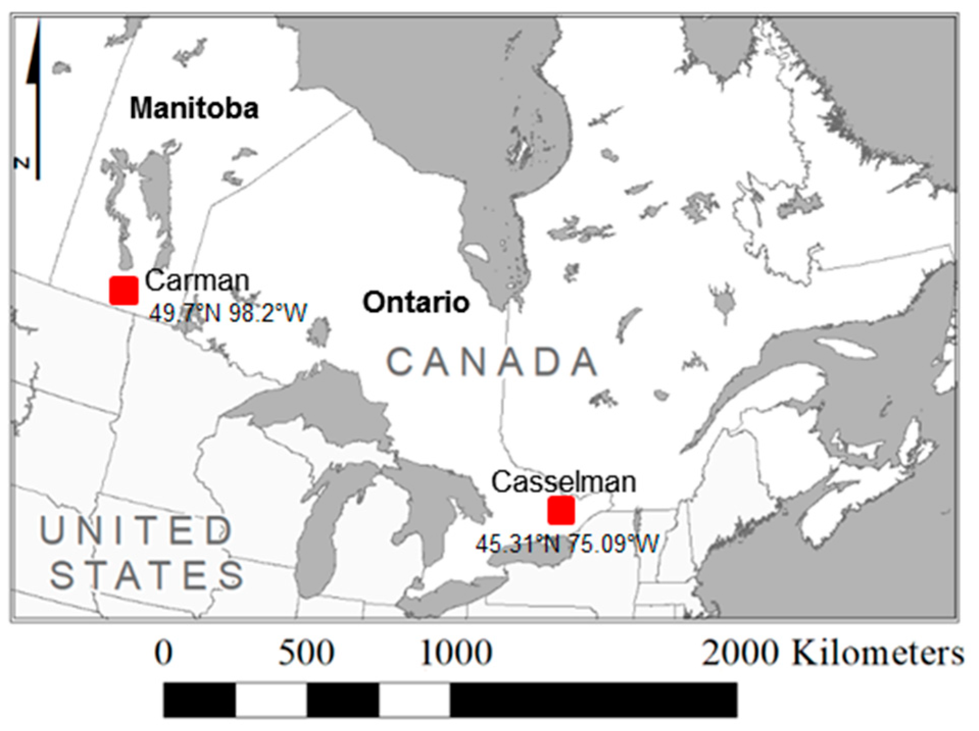
The in situ SMC measurements considered in this study were recorded by seven RISMA stations in the Carman area in 2015. These stations collect SMC data every 15 minutes [33]. Three sets of hydra probe sensors [34] are installed at each station to measure real dielectric permittivity, soil moisture, and soil temperature at 0–5 cm (vertical), 5 cm (horizontal), 20 cm (horizontal), 50 cm (horizontal), and 100 cm (horizontal). In our study, we considered the integrated SMC measured vertically from 0–5 cm. The RISMA data are collected by the Government of Canada through Agriculture and Agri-Food Canada and are available online [35]. A second intensive agriculture area was considered for assessing the proposed method on an independent dataset. This second area is located within the South Nation River watershed, close to the town of Casselman (45.31°N, 75.09°W), in eastern Ontario. The site is predominantly flat, except for a few elevation changes. A variety of soil types are present, including silty loam, sandy, and clay soils. This area is also equipped by another RISMA network of stations, providing the in situ SMC data to be used as reference. The location of the two test areas is shown in Figure 1.
On the Carman site, four sets of Fine Quad Wide (FQW) RADARSAT-2 polarimetric SAR images were acquired in 2015 on four dates between September and November during a period of bare soil and sparse vegetation (after the growing season). The list of images is provided in (Table 1). Each set contained six SAR images (total twenty-four images); three images in the satellite’s ascending orbit and three images in its descending orbit. The SAR incidence angle varies between ascending and descending orbits. Inspection of the archived weather information confirmed that there was no snowfall during the study period (25 September to 2 November) over the experimental site.
In the case of Casselman, two RS2 FQW images were acquired in November 2014 and June 2015, respectively (Table 1). Both images were acquired over bare soil conditions, since the first image (November 2014) was acquired after the growing season and the second image (June 2015) was acquired in the spring when crops were not present [36]. The bare soil conditions in June 2015 was further confirmed by considering the Normalized Difference Vegetation Index (NDVI) derived from the closest Landsat-8 L1TP image over Casselman in almost cloud free conditions, which was collected on 29 May 2015. The average NDVI value for the entire agricultural area was around 0.15, with minor changes from one field to another.
The RS2 polarimetric acquisitions (24 + 2) were processed by using a CP SAR simulator developed for the RADARSAT Constellation Mission (RCM) at the Canada Centre for Mapping and Earth Observation [36,37]. The simulator converts the RADARSAT-2 16-bit complex products to a 32-bit float complex according to the product documentation [38] by applying the sigma-nought calibration coefficients provided in the data files.
Since terrain correction was not applied due to the flat landscape of the study areas, the local incidence angle (LIA) was assumed equal to the nominal angle, from near to far range.
Then, the right circular transmit and linear horizontal receive (RH) and right circular transmit and linear vertical receive (RV) polarizations are calculated from the calibrated H or V transmitted, H or V received polarizations (HH, HV, VH, and VV). The RH and RV are converted to Stokes vector, which is then speckle filtered using a refined Lee filter with a 7 × 7 window size [39] and used for the extraction of 22 CP parameters that are listed in Table 2.
3. Data Analysis
3.1. Linear Polarization
The calibrated and geocoded σ° at the three polarizations (assuming HV = VH) available were compared with the in situ SMC measurements over the Carman site. The σ° values estimated at each station were co-located with the corresponding SMC recorded by the hydra probes at the time of satellite acquisition.
Considering the fine RS2 resolution, no upscaling/downscaling of data was needed to relate σ° to in situ SMC. The resulting dataset was composed of less than two hundred vectors of co-located σ°, CP parameters, and SMC that were considered for implementing and validating the algorithms.
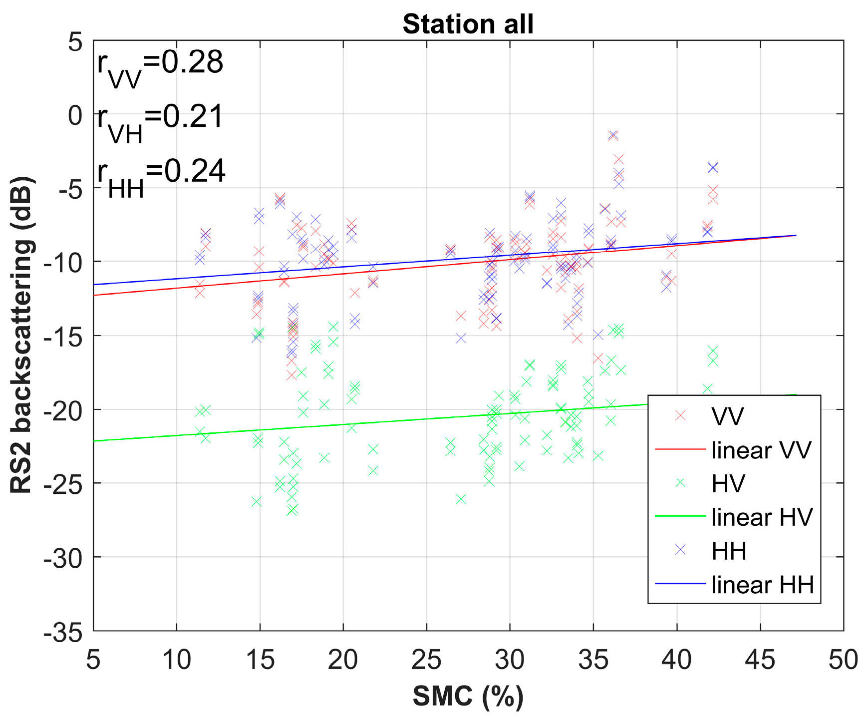
Figure 2 shows the scatterplot of σ° in VV, HH, and HV polarizations as a function of SMC. The high dispersion of σ° values for each SMC from in situ measurements could be attributed to the local surface features at each measurement point and in particular to soil texture and roughness, since the soils were bare or scarcely vegetated at the time of the RS2 acquisitions. The differences in observation geometry between RS2 data acquired in ascending and descending orbits also contributed to the data dispersion. The correlation of σ° to SMC was therefore weak; however, the plot in Figure 2 confirms the expected increasing behaviour of σ° when SMC increased. Furthermore, Figure 2 confirms the lower sensitivity of cross-polarized compared to co-polarized data to SMC, shown in terms of the correlation coefficients (r) values which vary between 0.21 in HV polarization to 0.28 in VV polarization.
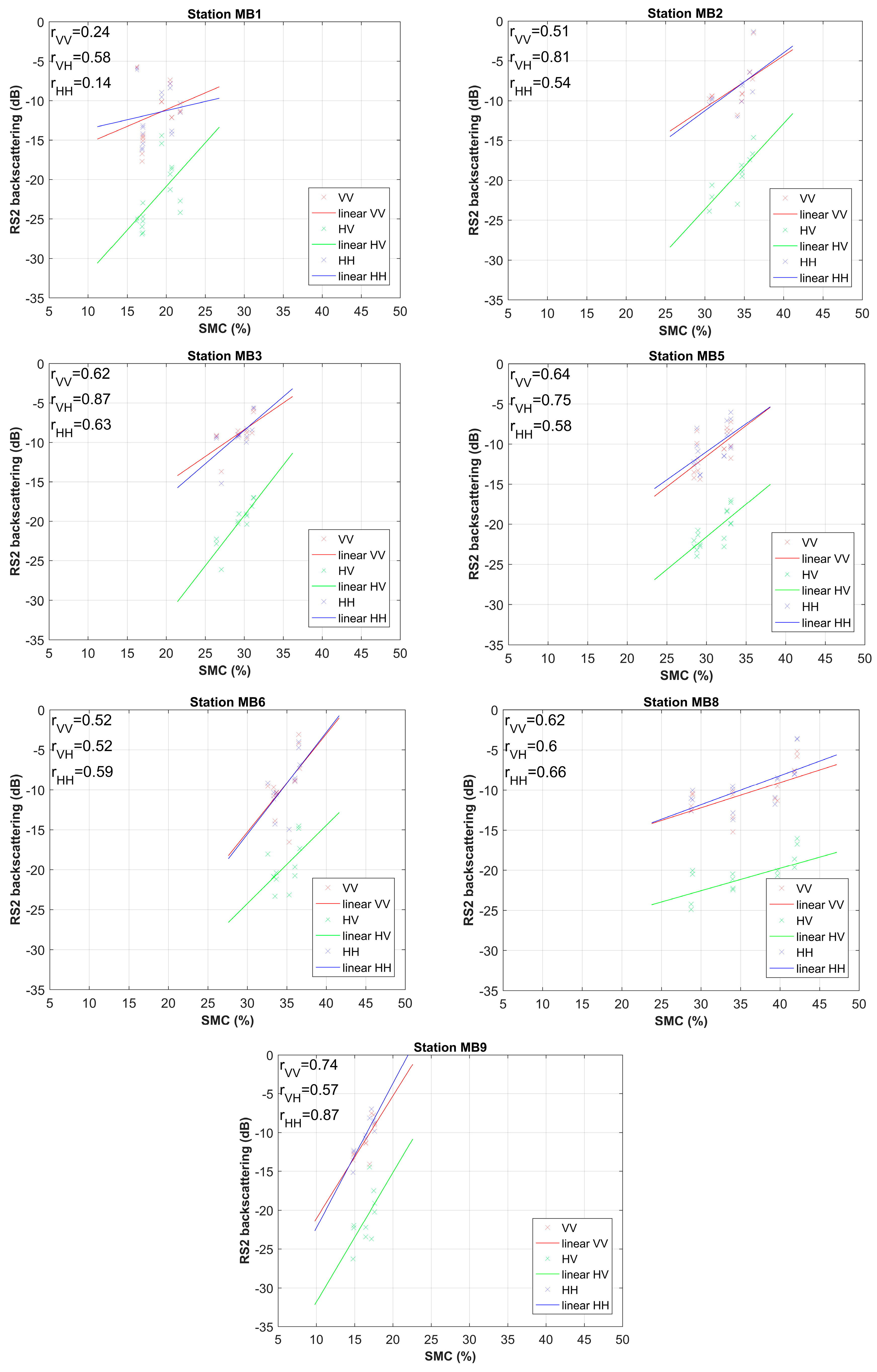
To verify the above observation and to better understand the effect of the spatial variability of the other surface parameters, the analysis was repeated by analysing independently the timeseries of data collected at each station. Examples of scatterplots σ° vs. SMC for the seven RISMA stations considered in this study are shown in Figure 3. The scatterplots confirm a difference in the relationship between σ° and SMC between the stations, as already reported by previous studies (e.g., Reference [11]). From the scatterplots it is evident the increasing trend of σ° at all polarizations with SMC; however, slopes and offsets of the regressions changed appreciably from one station to another.
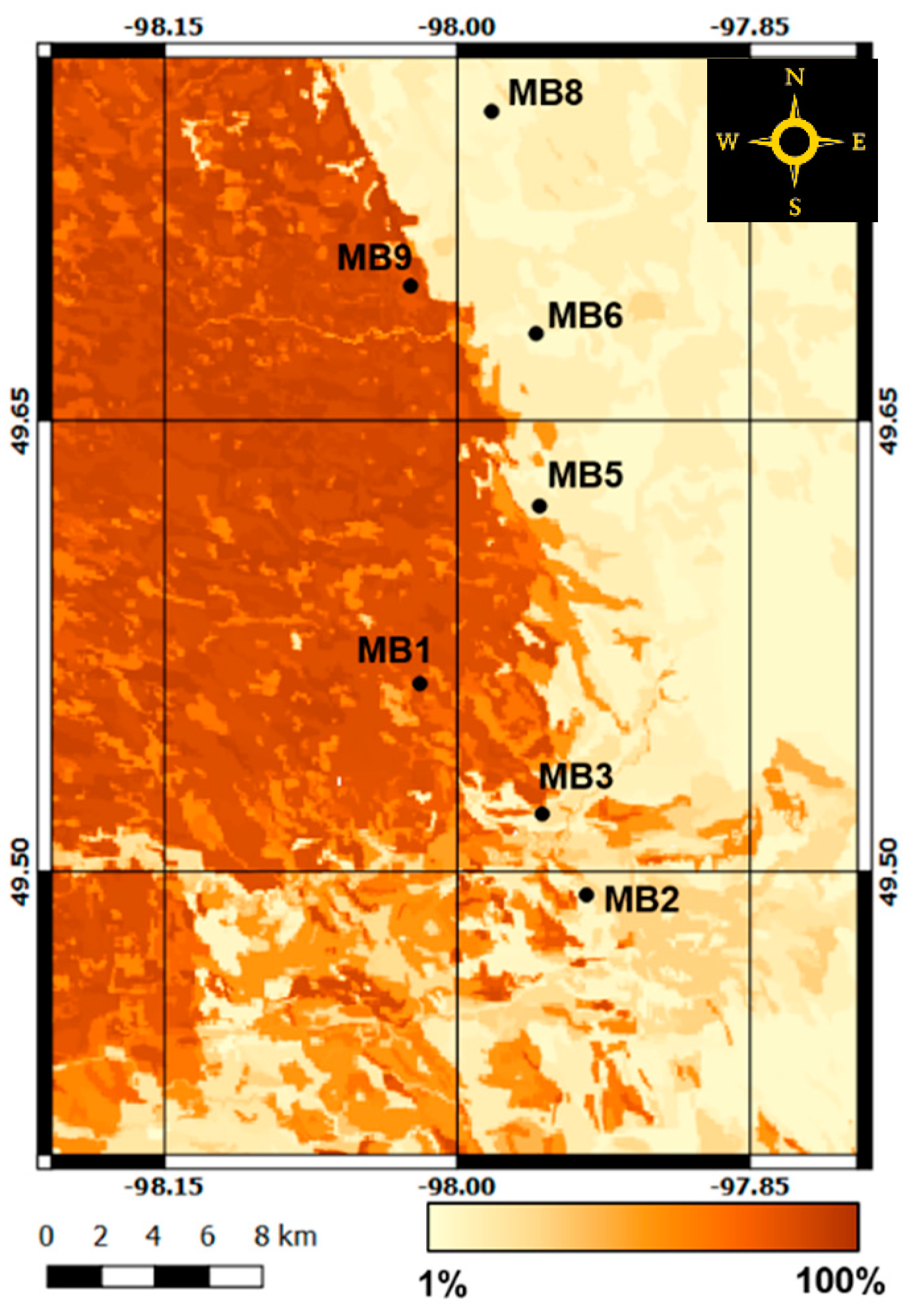
Since the experimental site is topographically flat and soils were bare or scarcely vegetated during the investigated time period, the effect of both local surface slopes and vegetation on the relationship between σ° and SMC was negligible. The data dispersion and the differences between stations could be therefore attributed to differences in soil texture, surface roughness, and observation geometry. Figure 4 shows the soil texture of the study area, expressed in sand percentage, with the location of the RISMA stations: darker shades indicate more sandy soil texture. In this respect, MB1 and MB9 were characterized by almost sandy soils, MB5, MB6, and MB8 had over 50% of clay, and MB2 and MB3 had a mixed type of sandy clay loam. The differences in soil texture affected the relationship between soil permittivity and SMC and therefore the one between σ° and SMC.
Considering the soil roughness, no direct measurements were available at the time of satellite acquisitions. However, data collected in 2012 and 2016 during two Soil Moisture Active Passive Validation Experiment (SMAPVEX) campaigns confirmed that differences existed between the stations in terms of correlation length and root mean square (RMS) height.
Concerning the viewing geometry, the existing differences between ascending and descending RS2 orbits lead to differences in the local incidence angle, which affect the radar backscattering, thus contribute to data dispersion.
3.2. Circular Polarization
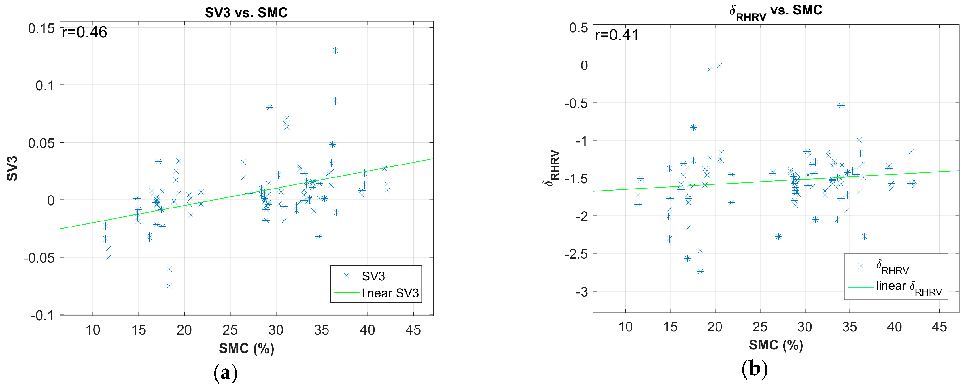
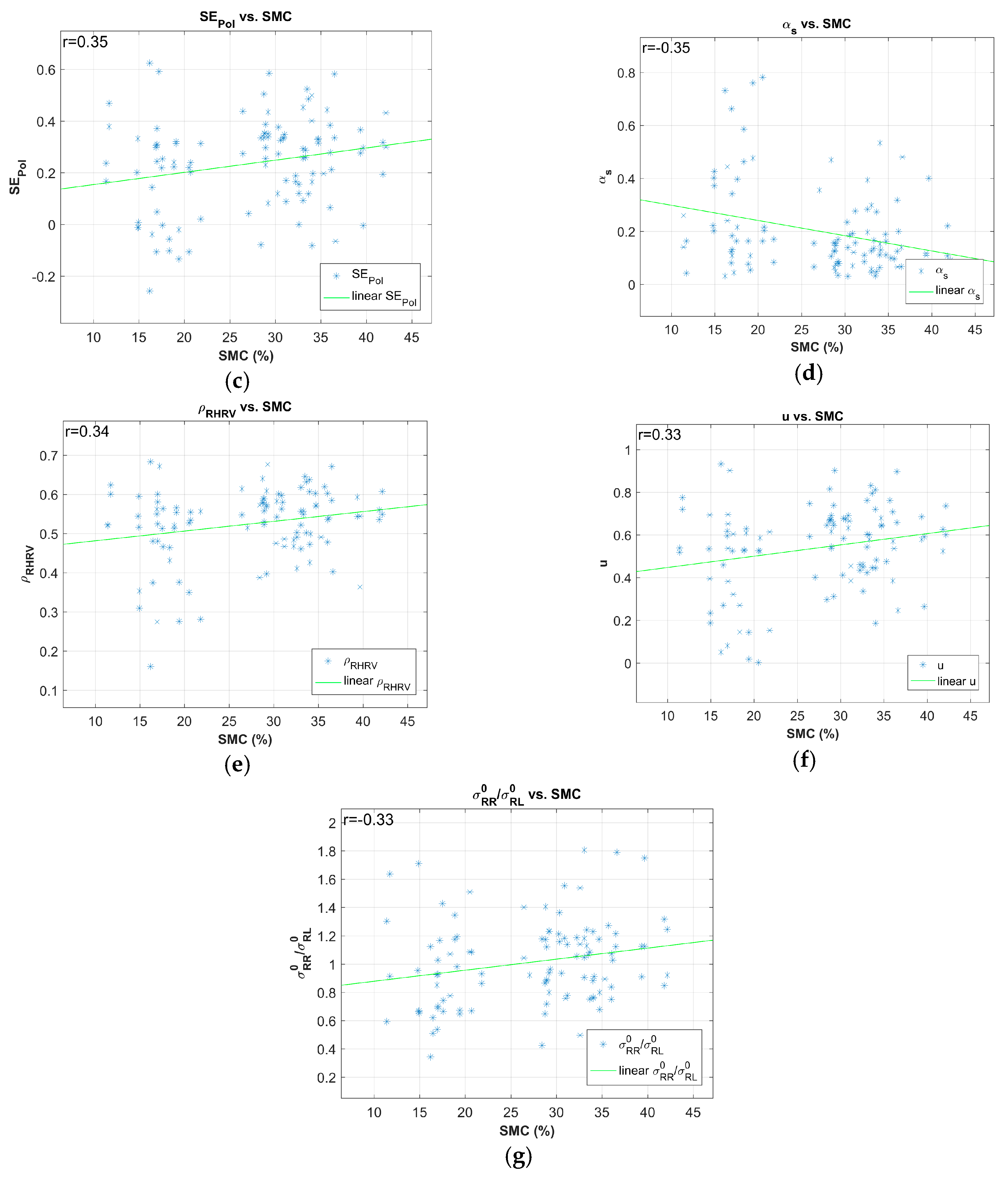
The sensitivity analysis was repeated for the CP parameters. Among the parameters generated by the simulator, the most correlated to SMC were the fourth component of Stokes vector (SV3), the RH–RV phase difference (), the Shannon entropy polarimetric component (SEPol), the alpha angle related to the ellipticity of the scattered wave (), the RH–RV correlation coefficient (), the conformity coefficient (u), and the circular polarization ratio . These seven parameters showed better correlation to SMC than σ°, as pointed out by the r values listed in Table 1. As shown in Table 3, in which the parameters better correlated to SMC than σ° are listed, all the CP parameters revealed positive correlation with the SMC, except for and which showed inverse relationships to SMC.
The highest correlation obtained by the SV3 parameter could be explained considering that the SV3 parameter was associated with the average power received in circular polarization and the polarized portion of the backscattered signal was dependent on SMC. The depolarized portion of the backscattered signal was instead triggered by other surface parameters, such as soil roughness or vegetation canopy. The other SV components reported r values similar to those obtained by σ°, and their worst performances could be simply attributed to the small dataset available. The correlation to SMC of parameter could be explained considering that contains information about the dielectric properties of the surface [46].
It should be also mentioned that the surface scattering mechanism from the m-delta or m-chi decomposition reported r values were similar to σ°. Conversely, the degree of polarization (m), which was indicated as a good descriptor of vegetation biomass in previous studies [47], did not show any significant correlation to SMC, since the increasing depolarization produced by the increasing biomass could not be observed on the scarcely vegetated surfaces of this study.
4. SMC Retrieval Algorithm Implementation
The obtained correlations, although encouraging, cannot be considered enough to attempt the retrieval with simple inversion methods. ML algorithms, based on artificial neural networks (ANN), were developed and trained for estimating SMC from several combinations of σ° and CP input parameters.
The inversion algorithms proposed here were based on feed-forward multi-layer perceptron (MLP) ANN, trained by using the back-propagation (BP) learning rule. MLP-ANN are composed of one input layer, one or more hidden layers, with a given number of neurons each, and one output layer. In MLP-ANN, neurons are connected with each other with adjustable weights and biases that can propagate the input data through the ANN similarly to the synapses in a biological brain. During the training, each input value is weighted and biased by adjustable coefficients and passed to the neurons of the first hidden layer. Here, it is added to the values coming from the other connections, multiplied by the transfer function and passed to the neurons of the second hidden layer (if present) or to the output layer. At each training iteration, the BP learning rule adjusts all the weight and bias coefficients for minimizing the mean square error (MSE) between predicted and target output values. The most common transfer functions are linear, hyperbolic tangent sigmoid (tansig), and log-sigmoid (logsig). Tansig returns an output value between −1 and 1 when the input value goes from −∞ to +∞, while Logsig output goes from 0 to 1 when a varies between −∞ and +∞.
The architecture definition and training have been made following the approach proposed in [12]. Analytically, an iterative processing that searches systematically for the optimal ANN architecture, in terms of neurons and hidden layers, has been implemented. The code starts from a very simple ANN configuration of one hidden layer with a number of neurons equal to the number of inputs. To reduce the risk of BP to find local minima of MSE, the training of each configuration is repeated 100 times, by resetting each time the ANN weights and biases to the initial values.
After each iteration, the trained ANN is applied to the test set and the resulting correlation coefficient (r) is computed. Then the neurons and hidden layers are iteratively increased up to a final configuration. Training and testing are repeated and r is again computed. The process is also iterated for the three available transfer functions; linear, logsig and tansig. Output is the ANN that obtained the highest r and should therefore represent the optimal configuration for solving the given problem. Training and validation have been carried out by splitting the available dataset 50:50, according to Reference [12]. The training set is further subsampled randomly in 60%, 20%, and 20% subsets: the first subset serves for iteratively adjusting the ANN weights and biases using BP; and the second and third subsets are used for having two a posteriori tests on independent subsets at each training iteration. Based on the so-called “early stopping” rule, the training stops as soon as the errors on the three subsets are diverging, in order to prevent overfitting. After training, the ANN was validated by predicting SMC on the remaining set of 50% data, not involved in the training.
Several combinations of CP parameters were considered for implementing the algorithms. In particular, the CP parameters listed in Table 1 were increasingly added to the ANN inputs and the training and validation processes were repeated, in order to point out the contribution of each CP parameter to the overall retrieval accuracy.
Two more ANN implementations, using the linear σ° values at VV + HV and VV + HH + HV polarizations were also implemented, trained and validated on the same dataset for comparison.
5. Results
5.1. ANN Algorithm Validation
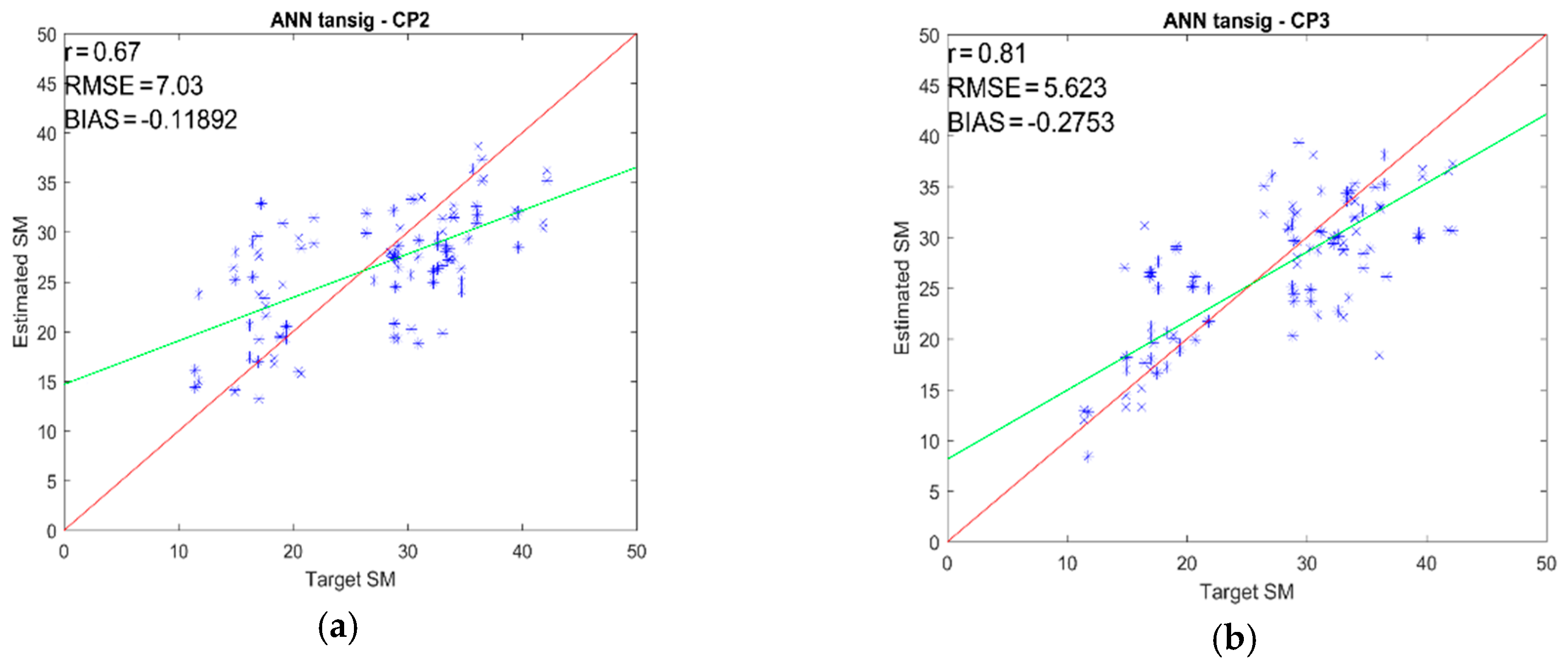
Figure 7 shows the validation of the ANN algorithms considering the following combinations of CP input parameters shown in Table 4. The results were obtained by applying the trained ANN to the validation set, which was composed of 50% of the available dataset (less than one hundred data vectors).
A larger dataset would be necessary to draw general conclusions. However, the obtained results were statistically significant, since p-value was <0.05 in all cases. Therefore, reasonable conclusions could be drawn. As shown in Table 4, all the combinations with more than two inputs were able to estimate SMC with correlation of around 0.8 and root mean square error lower than 6%. By comparing the ANN with the same number of inputs (two and three), the ANN fed by CP parameters (CP2 and CP3) slightly better results were returned than the corresponding fed by linearly polarized σ° (2pol and 3pol). This indicated that the information contained in CP parameters was higher than that contained in σ°, as also is confirmed by the higher correlations to SMC pointed out by Table 1.
It should be also mentioned that an attempt to include the VH pol. (along with the HV pol.) to the ANN inputs did not cause any improvement in the retrievals based on linearly polarized backscattering.
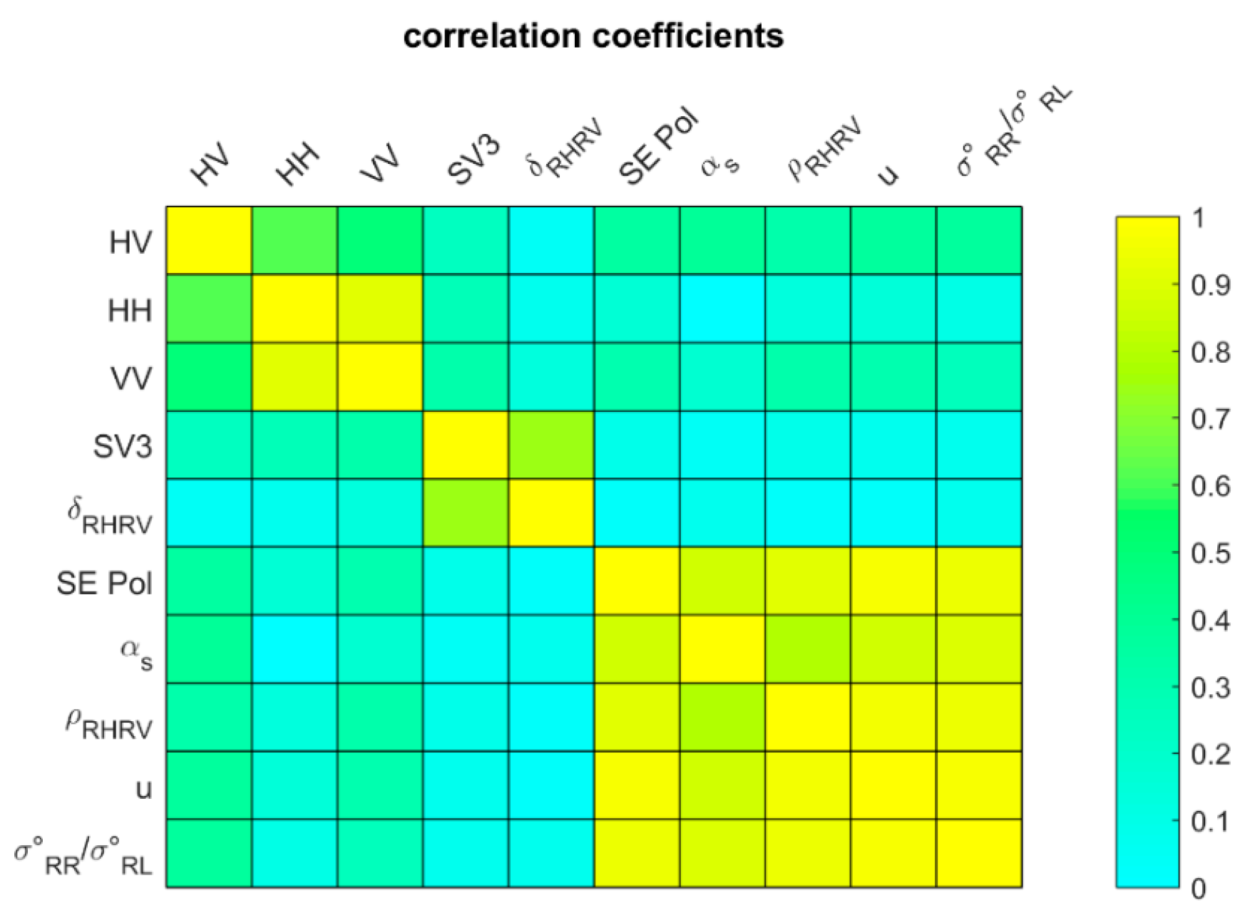
Table 4 shows that the inclusion of the to the combination of SV3 and remarkably improved the correlation r from 0.67 to 0.81 and reduced the RMSE from 7.03% to 5.62% for CP2 and CP3, respectively. This is explained by the correlation plot in Figure 6, which shows that the parameter was less correlated (<0.5) with the two CP parameters SV3 and . Thus, the inclusion of this parameter () contributed significantly with additional information which improved the SMC retrieval. The inclusion of additional parameters from CP4 to CP7 improved slightly the values of the correlation and the RMSE. This was due to the fact that the CP parameters SEPol, , u, and were highly correlated (>0.5) with the parameter, as shown in Figure 6. The contribution of these parameters with additional information about the SMC to the CP4 combination is therefore limited.
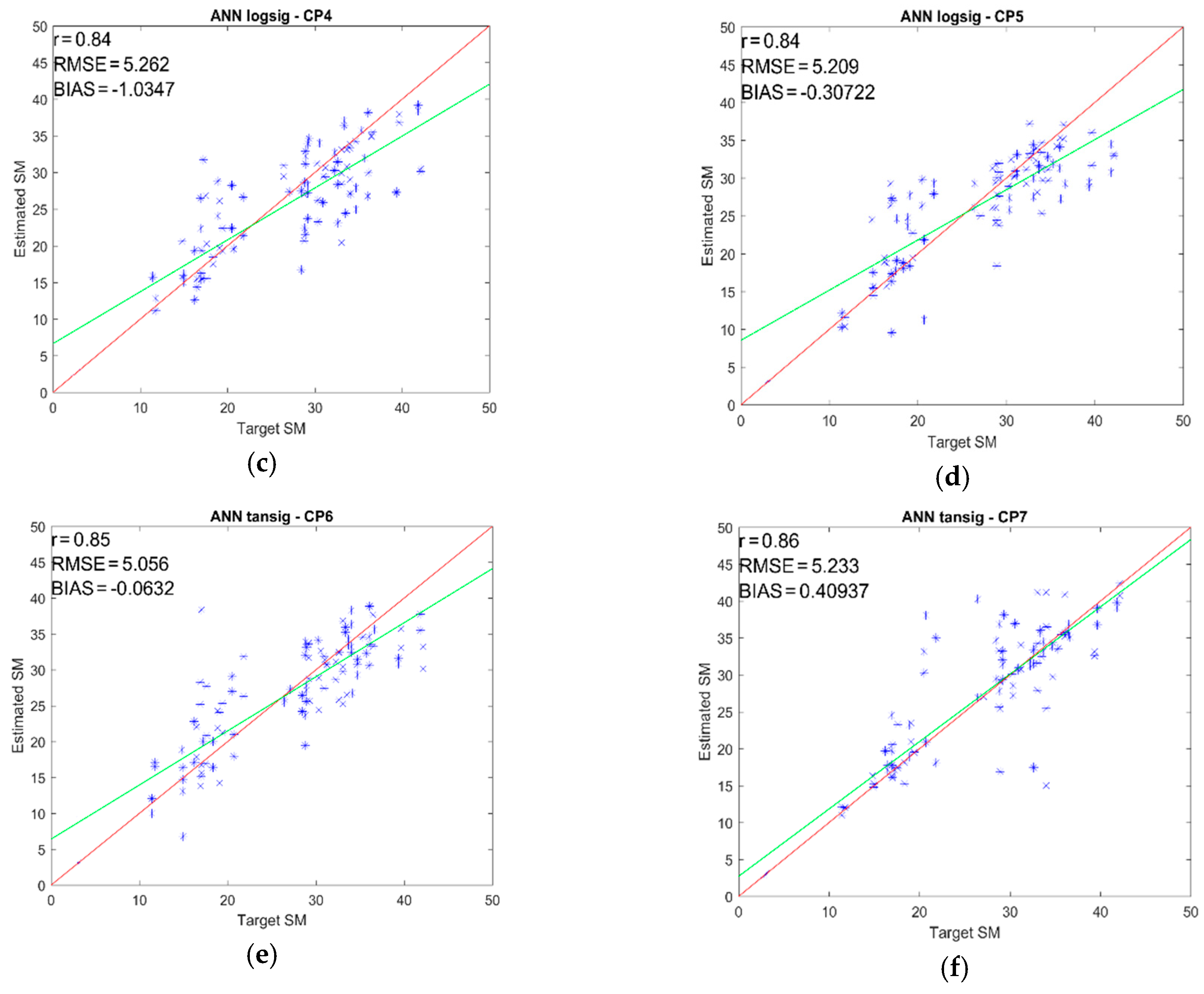
The scatterplots of the ANN estimated vs. target SMC on the validation set for the combinations CP2–CP7 are shown in Figure 7a–f, while the results for the 2pol and 3pol configurations are shown in Figure 8a,b. The information on the “best” transfer function used, depending on the systematic ANN optimization described in Section 4 is also reported in the plots.
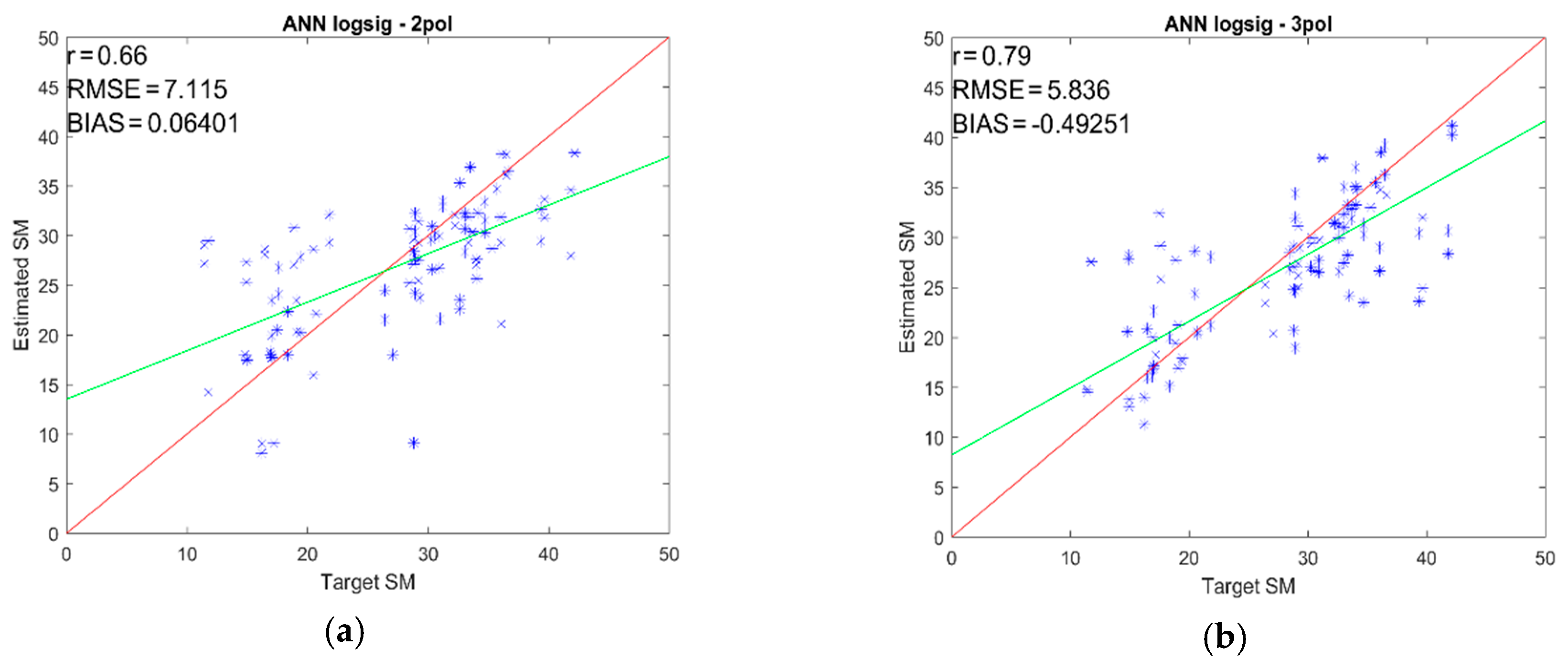
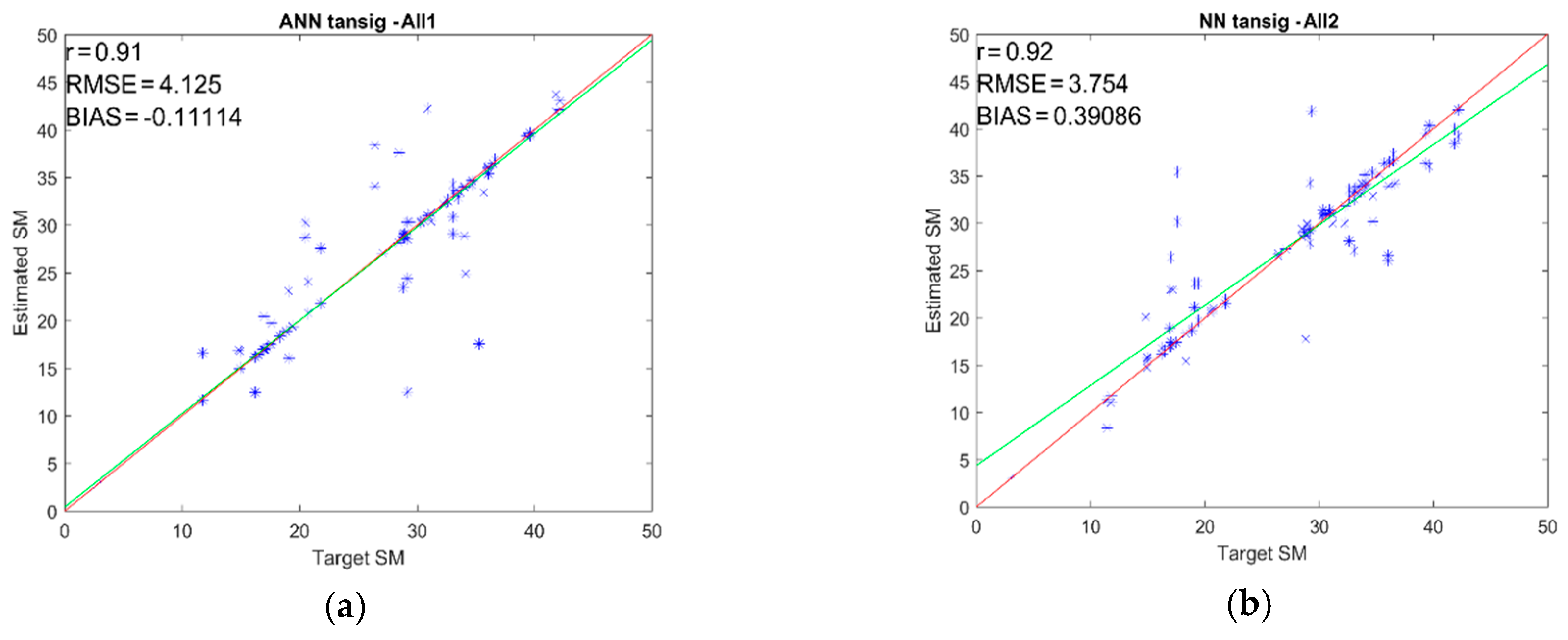
A further attempt to improve the retrievals was carried out by combining the linearly polarized σ° and the CP parameters. Among all the possible combinations, the best results were obtained by the All1 and All2 reported in Table 4. With these two combinations, the retrieval of SMC was possible with r > 0.9 and RMSE ≃ 4 (% of SMC). Small differences were found between the results of All1 and All2 combinations. This indicates that most of the information related to SMC was already included in the All1 combination of parameters. The corresponding scatterplots are shown in Figure 9a,b.
5.2. Independent Test on Casselman
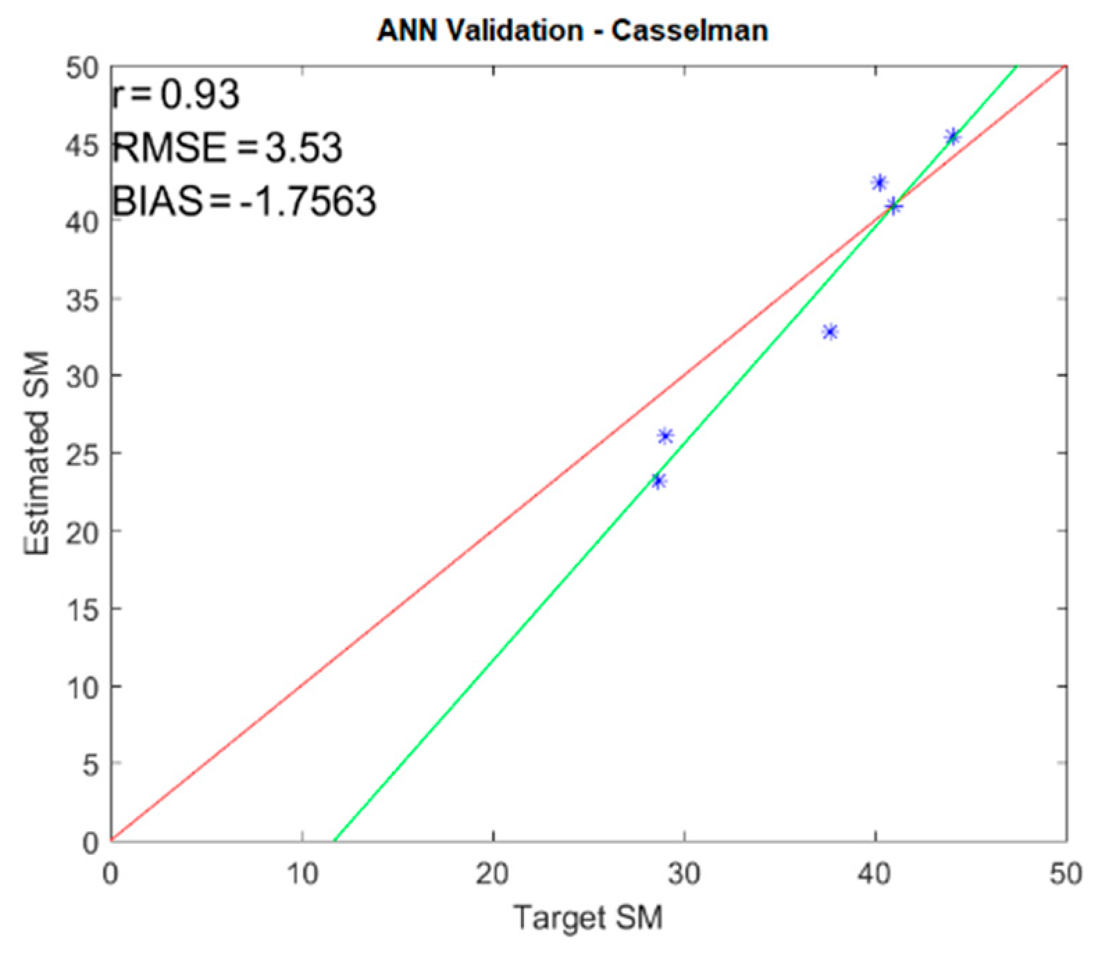
The ANN algorithm, trained and validated on Carman data, has been applied to the data collected on the Casselman test area, for which in situ SMC data were available from four RISMA stations. The obtained scatterplot from the implementation of the algorithm using the ANN All2 (σ° + CP) is shown in Figure 10. Unfortunately, the dataset was small (six points only, since two stations fall out of the June image), and therefore the statistical significance of the test was poor. However, the result seemed to be suggesting that the algorithm trained with Carman data could be applied to another test site (Casselman), which was not used for training the algorithm. The algorithm achieved a high correlation between measured and retrieved SMC equal to 0.93 with a small RMSE equal to 3.5%.
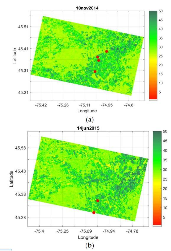
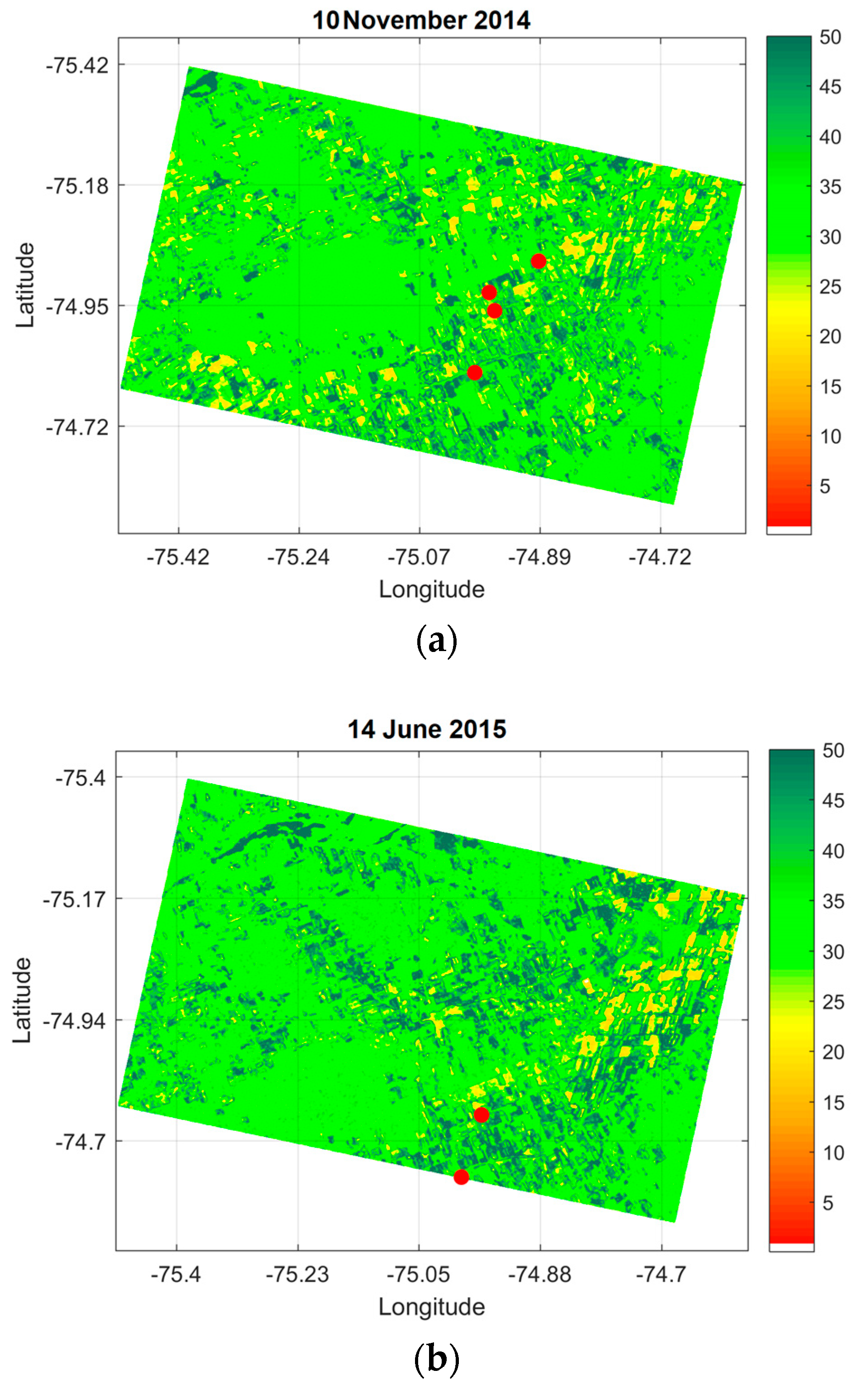
SMC maps were generated by applying the All2 ANN algorithm to the entire RS2 images. Figure 11 shows two examples of SMC maps of the Casselman test site obtained by applying the ANN algorithm pixel by pixel. The maps were validated on the locations of RISMA stations, shown on the maps as red dots, and the general trend agreed with the in situ information available on the area at the dates of the RS2 acquisitions.
6. Discussion
The comparison between σ°, CP parameters, and SMC demonstrated that some CP parameters are better related to SMC than linearly polarized σ°, thus suggesting that the CP parameters have a good potential in improving the accuracy of SMC retrievals from SAR acquisitions. This was indeed confirmed by the validation results shown in Figure 7 and Figure 8, in which the ANN based on CP parameters outperformed the corresponding ANN based on linearly polarized σ°.
The different response of each SAR parameter to the surface features was able compensate for the effect of surface conditions on the relationships between SAR observations and SMC computed at local stations, as shown in Figure 3 [11].
The obtained results confirmed that the more input SAR parameters were considered for retrieving SMC, the more the retrieval accuracy was improved, as demonstrated by the validation results summarized in Table 4. The correlation coefficient increased from r = 0.67 of the retrievals obtained with two inputs up to r = 0.92 for the merged CP + σ° in the ANN implementations All1 and All2 (Figure 9), while the corresponding RMSE decreased from 7 (% of SMC) to 3.8 (% of SMC).
It should be mentioned that the main contribution to these results was given by the first three CP parameter listed in Table 1, while the contribution of the remaining CP parameters was less important.
However, these results were obtained on a relatively small set of data, and therefore should be verified on larger datasets. The encouraging results obtained on Casselman indicated promising possibility to apply the algorithm to experimental sites other than those for which it has been developed. The site dependency is in any case a characteristic of all “data driven” approaches, since the datasets derived from experimental activities refer to particular environmental conditions and their representativeness for other areas and different environments has to be verified [12]. To reduce such site dependency, the ANN training should be updated by including data representative of all the considered sites. Updating the training is anyway quite straightforward and it can be achieved without modifying the algorithm structure each time new datasets are available. This represents a unique feature of the data driven approaches based on ML, compared to conventional inversions of electromagnetic forward models.
7. Conclusions
This study was aimed at demonstrating the joint use of machine learning (ML) and compact polarimetry (CP) for improving the retrieval of surface soil moisture (SMC) from SAR acquisitions at C-band. The study was conducted on two agricultural areas in Canada, for which time-series of RADARSAT-2 (RS2) images were available along with direct measurements of SMC from in situ stations. Linearly polarized backscatter coefficients (σ°) were related to SMC, confirming the expected increase when SMC increased. However, the correlation was low (0.21 ≤ r ≤ 0.28), possibly depending on the variability of other surface parameters such as the soil texture and surface roughness, as well as the different acquisition geometry of RS2 in ascending and descending orbits. CP data generated from the RS2 acquisitions using a CP simulator, indicated that seven CP parameters out of a set of 22 examined parameters were better correlated to SMC than the linear σ° (0.33 ≤ r ≤ 0.46).
The obtained correlations, although encouraging, cannot be considered enough to attempt the retrieval with simple inversion methods. ML algorithms, based on artificial neural networks (ANN), were developed and trained for estimating SMC from several combination of σ° and CP input parameters. The validation of the algorithm with in situ observations confirmed the promising capabilities of the ML approaches for SMC monitoring, especially when applied to multiple polarizations. The proposed ANN algorithm was able to achieve retrieved SMC with correlation from 0.67 to 0.92 and RMSE from 7% to 3.8% with in situ measured SMC.
Author Contributions
data curation, M.D. and S.P. (Simone Pettinato); formal analysis, E.S.; investigation, M.D. and E.S.; methodology, E.S. and S.P. (Simonetta Paloscia); resources, M.D.; software, E.S.; supervision, S.P. (Simonetta Paloscia) and S.P. (Simone Pettinato); validation, S.P. (Simone Pettinato); writing—original draft, E.S.; writing—review and editing, M.D. and S.P. (Simonetta Paloscia).
Funding
This research received no external funding.
Acknowledgments
The authors would like to thank the Canada Center of Remote Sensing for providing the CP SAR simulator. This work was supported by the Italian and Canadian Space Agencies (ASI and CSA), which provided the necessary SAR images through the proposal ASI-SOAR-PI2880/5225. RADARSAT-2 data and products © MacDonald, Dettwiler and Associates Ltd. (2013)—All Rights Reserved. RADARSAT is an official mark of the Canadian Space Agency.
Conflicts of Interest
The authors declare no conflict of interest.
References
- Narvekar, P.S.; Entekhabi, D.; Kim, S.; Njoku, E.G. Soil Moisture Retrieval Using L-Band Radar Observations. IEEE Trans. Geosci. Remote Sens. 2015, 53, 3492–3506. [Google Scholar] [CrossRef]
- Shi, J.C.; Wang, J.; Hsu, A.Y.; O’Neill, P.E.; Engman, E.T. Estimation of bare surface soil moisture and surface roughness parameter using L-band SAR image data. IEEE Trans. Geosci. Remote Sens. 1997, 35, 1254–1266. [Google Scholar] [CrossRef]
- Shi, J.; Jackson, T.; Tao, J.; Du, J.; Bindlish, R.; Lu, L.; Chen, K.S. Microwave vegetation indices for short vegetation covers from satellite passive microwave sensor AMSR-E. Remote Sens. Environ. 2008, 112, 4285–4300. [Google Scholar] [CrossRef]
- Macelloni, G.; Paloscia, S.; Pampaloni, P.; Sigismondi, S.; de Matthæis, P.; Ferrazzoli, P.; Schiavon, G.; Solimini, D. The SIR-C/X-SAR experiment on Montespertoli: Sensitivity to hydrological parameters. Int. J. Remote Sens. 1999, 20, 2597–2612. [Google Scholar] [CrossRef]
- Ulaby, F.T.; Moore, R.K.; Fung, A.K. Microwave Remote Sensing: Active and Passive; Artech House: Norwood, MA, USA, 1986; Volume III. [Google Scholar]
- Santi, E.; Paloscia, S.; Pettinato, S.; Brocca, L.; Ciabatta, L.; Entekhabi, D. On the synergy of SMAP, AMSR2 and SENTINEL-1 for retrieving soil moisture. Int. J. Appl. Earth Obs. Geoinf. 2018, 65, 114–123. [Google Scholar] [CrossRef]
- Balenzano, A.; Mattia, F.; Satalino, G.; Davidson, M.W.J. Dense Temporal Series of C- and L-band SAR Data for Soil Moisture Retrieval over Agricultural Crops. IEEE JSTARS 2011, 4, 439–450. [Google Scholar] [CrossRef]
- Bauer-Marschallinger, B.; Freeman, V.; Cao, S.; Paulik, C.; Schaufler, S.; Stachl, T.; Modanesi, S.; Massari, C.; Ciabatta, L.; Brocca, L.; et al. Toward Global Soil Moisture Monitoring with Sentinel-1: Harnessing Assets and Overcoming Obstacles. IEEE Trans. Geosci. Remote Sens. 2019, 57, 520–539. [Google Scholar] [CrossRef]
- Wagner, W.; Lemoine, G.; Rott, H. A method for estimating soil moisture from ERS scatterometer and soil data. Remote Sens. Environ. 1999, 70, 191–207. [Google Scholar] [CrossRef]
- Bartalis, Z.; Wagner, W.; Naeimi, V.; Hasenauer, S.; Scipal, K.; Bonekamp, H.; Figa, J.; Anderson, C. Initial soil moisture retrievals from the METOP-A Advanced Scatterometer (ASCAT). Geophys. Res. Lett. 2007, 34, L20401. [Google Scholar] [CrossRef]
- Paloscia, S.; Pettinato, S.; Santi, E.; Notarnicola, C.; Pasolli, L.; Reppucci, A. Soil moisture mapping using Sentinel-1 images: Algorithm and preliminary validation. Remote Sens. Environ. 2013, 134, 234–248. [Google Scholar] [CrossRef]
- Santi, E.; Paloscia, S.; Pettinato, S.; Fontanelli, G. Application of artificial neural networks for the soil moisture retrieval from active and passive microwave spaceborne sensors. Int. J. Appl. Earth Observ. Geoinf. 2016, 48, 61–73. [Google Scholar] [CrossRef]
- Chen, S.W.; Li, Y.Z.; Wang, X.S.; Xiao, S.P. Modeling and Interpretation of Scattering Mechanisms in Polarimetric Synthetic Aperture Radar: Advances and Perspectives. Signal Process. Mag. 2014, 31, 79–89. [Google Scholar] [CrossRef]
- Baghdadi, N.; Cresson, R.; Pottier, E.; Aubert, M.; Zribi, M.; Jacome, A.; Benabdallah, S. A Potential Use for the C-Band Polarimetric SAR Parameters to Characterize the Soil Surface over Bare Agriculture Fields. IEEE Trans. Geosci. Remote Sens. 2012, 50, 3844–3858. [Google Scholar] [CrossRef]
- Baghdadi, N.; Dubois-Fernandez, P.; Dupuis, X.; Zribi, M. Sensitivity of Main Polarimetric Parameters of Multifrequency Polarimetric SAR Data to Soil Moisture and Surface Roughness over Bare Agricultural Soils. IEEE Geosci. Remote Sens. Lett. 2013, 10, 731–735. [Google Scholar] [CrossRef]
- Pasolli, L.; Notarnicola, C.; Bruzzone, L.; Bertoldi, G.; Chiesa, S.D.; Niedrist, G.; Tappeiner, U.; Zebisch, M. Polarimetric Radarsat-2 Imagery for Soil Moisture Retrieval in Alpine Areas. Can. J. Remote Sens. 2012, 37, 535–547. [Google Scholar] [CrossRef]
- Hajnsek, I.; Jagdhuber, T.; Schön, H.; Papathanassiou, K.P. Potential of Estimating Soil Moisture under Vegetation Cover by Means of PolSAR. IEEE Trans. Geosci. Remote Sens. 2009, 47, 442–454. [Google Scholar] [CrossRef]
- Hajnsek, I.; Pottier, E.; Cloude, S. Inversion of Surface Parameters from Polarimetric SAR. IEEE Trans. Geosci. Remote Sens. 2003, 41, 727–744. [Google Scholar] [CrossRef]
- Trudel, M.; Charbonneau, F.; Leconte, R. Using Radarsat-2 Polarimetric and ENVISATASAR Dual-Polarization Data for Estimating Soil Moisture over Agricultural Fields. Can. J. Remote Sens. 2012, 38, 514–527. [Google Scholar] [CrossRef]
- Notarnicola, C. A Bayesian Change Detection Approach for Retrieval of Soil Moisture Variations Under Different Roughness Conditions. IEEE Geosci. Remote Sens. Lett. 2014, 11, 414–418. [Google Scholar] [CrossRef]
- Pierdicca, N.; Pulvirenti, L.; Pace, G. A Prototype Software Package to Retrieve Soil Moisture from Sentinel-1 Data by Using a Bayesian Multitemporal Algorithm. IEEE J. Sel. Top. Appl. Earth Obs. Remote Sens. 2014, 7, 153–163. [Google Scholar] [CrossRef]
- Pasolli, L.; Notarnicola, C.; Bertoldi, G.; Bruzzone, L.; Remelgado, R.; Greifeneder, F.; Niedrist, G.; Della Chiesa Tappeiner, U.; Zebisch, M. Estimation of Soil Moisture in Mountain Areas Using SVR Technique Applied to Multiscale Active Radar Images at C-Band. IEEE J. Sel. Top. Appl. Earth Obs. Remote Sens. 2015, 8. [Google Scholar] [CrossRef]
- Hornik, K.; Stinchcombe, M.; White, H. Multilayer feed forward network are universal approximators. Neural Netw. 1989, 2, 359–366. [Google Scholar] [CrossRef]
- Linden, A.; Kinderman, J. Inversion of multi-layer nets. Proc. Int. Jt. Conf. Neural Netw. 1989, 2, 425–443. [Google Scholar] [CrossRef]
- Del Frate, F.; Ferrazzoli, P.; Schiavon, G. Retrieving soil moisture and agricultural variables by microwave radiometry using neural networks. Remote Sens. Environ. 2003, 84, 174–183. [Google Scholar] [CrossRef]
- Elshorbagy, A.; Parasuraman, K. On the relevance of using artificial neural networks for estimating soil moisture content. J. Hydrol. 2008, 362, 1–18. [Google Scholar] [CrossRef]
- Paloscia, S.; Pampaloni, P.; Pettinato, S.; Santi, E. A Comparison of Algorithms for Retrieving Soil Moisture From ENVISAT/ASAR Images. IEEE Trans. Geosci. Remote Sens. 2008, 46, 3274–3284. [Google Scholar] [CrossRef]
- Thomas, B. An Essay towards solving a Problem in the Doctrine of Chances. By the late Rev. Mr. Bayes, F.R.S. communicated by Mr. Price, in a letter to John Canton, A.M.F.R.S. Philos. Trans. R. Soc. Lond. 1763, 53, 370–418. [Google Scholar] [CrossRef]
- Nelder, J.A.; Mead, R. A Simplex Method for Function Minimization. Comput. J. 1965, 7, 308–313. [Google Scholar] [CrossRef]
- Baghdadi, N.; Cresson, R.; El Hajj, M.; Ludwig, R.; La Jeunesse, I. Estimation of soil parameters over bare agriculture areas from C-band polarimetric SAR data using neural networks. Hydrol. Earth Syst. Sci. 2012, 16, 1607–1621. [Google Scholar] [CrossRef] [Green Version]
- McNairn, H.; Jackson, T.J.; Wiseman, G.; Belair, S.; Berg, A.; Bullock, A.; Colliander, A.; Cosh, M.H.; Kim, S.-B.; Magagi, R.; et al. The soil moisture active passive validation experiment 2012 (SMAPVEX12): Prelaunch Calibration and Validation of the SMAP Soil Moisture Algorithms. IEEE Trans. Geosci. Remote Sens. 2015, 53, 2784–2801. [Google Scholar] [CrossRef]
- Dabboor, M.; Leqiang, S.; Carrera, M.L.; Friesen, M.; Merzouki, A.; McNairn, H.; Powers, J.; Baclair, S. Comparative Analysis of High-Resolution Soil Moisture Simulations from the Soil, Vegetation, and Snow (SVS) Land Surface Model Using SAR Imagery Over Bare Soil. Water 2019, 11, 542. [Google Scholar] [CrossRef]
- Sun, L.; Dabboor, M.; Belair, S.; Carrera, M.L.; Merzouki, A. Simulating C-band SAR footprint-scale backscatter over agricultural area with a physical land surface model. Water Resour. Res. 2019, 55, 4594–4612. [Google Scholar] [CrossRef]
- Pacheco, A.; L’Heureux, J.; McNairn, H.; Powers, J.; Howard, A.; Geng, X.; Rollin, P.; Gottfried, K.; Freeman, J.; Ojo, R.; et al. Real-Time in-Situ Soil Monitoring for Agriculture (RISMA) Network Metadata, AAFC. Available online: https://agriculture.canada.ca/SoilMonitoringStations/files/RISMA_Network_Metadata.pdf (accessed on 21 October 2019).
- Government of Canada. Available online: https://agriculture.canada.ca/SoilMonitoringStations/historical-data-en.html (accessed on 21 October 2019).
- Merzouki, A.; McNairn, H.; Powers, J.; Friesen, M. Synthetic Aperture Radar (SAR) Compact Polarimetry for Soil Moisture Retrieval. Remote Sens. 2019, 11, 2227. [Google Scholar] [CrossRef]
- Dabboor, M.; Geldsetzer, T. Towards sea ice classification using simulated RADARSAT constellation mission compact polarimetric SAR imagery. Remote Sens. Environ. 2014, 140, 189–195. [Google Scholar] [CrossRef]
- MAXAR. Available online: https://mdacorporation.com/docs/default-source/technical-documents/geospatial-services/radarsat-2-product-format-definition.pdf?sfvrsn=4 (accessed on 21 October 2019).
- Lee, J.S.; Pottier, E. Polarimetric Radar Imaging: From Basics to Applications; CRC Press: Boca Raton, FL, USA, 2009. [Google Scholar] [CrossRef]
- Raney, R.K.; Cahill, J.T.S.; Patterson, G.W.; Bussey, D.B. The m-chi decomposition of hybrid dual-polarimetric radar data with application to lunar craters. J. Geophys. Res. 2012, 117, E00H21. [Google Scholar] [CrossRef]
- Réfrégier, P.; Morio, J. Shannon entropy of partially polarized and partially coherent light with Gaussian fluctuations. J. Opt. Soc. Am. A 2006, 23, 3036–3044. [Google Scholar] [CrossRef]
- Raney, R.K. Hybrid-polarity SAR architecture. IEEE Trans. Geosci. Remote Sens. 2007, 45, 3397–3404. [Google Scholar] [CrossRef]
- Charbonneau, F.; Brisco, B.; Raney, K.; McNairn, H.; Liu, C.; Vachon, P.; Shang, J.; DeAbreu, R.; Champagne, C.; Merzouki, A.; et al. Compact polarimetry overview and applications assessment. Can. J. Remote Sens. 2010, 36, S298–S315. [Google Scholar] [CrossRef]
- Truong-Loi, M.; Freeman, A.; Dubois-Fernandez, P.; Pottier, E. Estimation of soil moisture and Faraday rotation from bare surfaces using compact polarimetry. IEEE Trans. Geosci. Remote Sens. 2009, 47, 3608–3615. [Google Scholar] [CrossRef]
- Cloude, S.R.; Goodenough, D.G.; Chen, H. Compact decomposition theory. IEEE Geosci. Remote Sens. Lett. 2012, 9, 28–32. [Google Scholar] [CrossRef]
- Ponnurangam, G.G.; Jagdhuber, T.; Hajnsek, I.; Rao, Y.S. Soil Moisture Estimation Using Hybrid Polarimetric SAR Data of RISAT-1. IEEE Trans. Geosci. Remote Sens. 2016, 54, 2033–2049. [Google Scholar] [CrossRef]
- Chang, J.G.; Shoshany, M.; Oh, Y. Polarimetric Radar Vegetation Index for Biomass Estimation in Desert Fringe Ecosystems. IEEE Trans. Geosci. Remote Sens. 2018, 56, 7102–7108. [Google Scholar] [CrossRef]
Figure 1.
Carman and Casselman test areas.

Figure 2.
Scatterplots of backscattering (σ°) at the Real-time In Situ Soil Monitoring for Agriculture (RISMA) station locations against the measured soil moisture content (SMC) in each station.
Figure 2.
Scatterplots of backscattering (σ°) at the Real-time In Situ Soil Monitoring for Agriculture (RISMA) station locations against the measured soil moisture content (SMC) in each station.

Figure 3.
Scatterplots of linearly polarized σ° as a function of SMC at the RISMA stations.

Figure 4.
Soil texture map expressed as sand percentage for the Carman site.

Figure 5.
CP parameter vs. in situ SMC: (a) SV3, (b) δRHRV, (c) αs, (d) ρRHRV, (e) σRR /σRL, (f) SEPol, and (g) u.
Figure 5.
CP parameter vs. in situ SMC: (a) SV3, (b) δRHRV, (c) αs, (d) ρRHRV, (e) σRR /σRL, (f) SEPol, and (g) u.


Figure 6.
Cross-correlation matrix of CP and σ° parameters. Colours are proportional to r values.

Figure 7.
ANN estimated vs. in situ SMC for the different combinations of CP parameters: (a) CP2, (b) CP3, (c) CP4, (d) CP5, (e) CP6, and (f) CP7.
Figure 7.
ANN estimated vs. in situ SMC for the different combinations of CP parameters: (a) CP2, (b) CP3, (c) CP4, (d) CP5, (e) CP6, and (f) CP7.


Figure 8.
ANN estimated vs. in situ SMC for the two different combinations of input σ°: (a) 2pol and (b) 3pol.
Figure 8.
ANN estimated vs. in situ SMC for the two different combinations of input σ°: (a) 2pol and (b) 3pol.

Figure 9.
ANN estimated vs. in situ SMC for the two different combinations of input σ° + CP: (a) All1 and (b) All2.
Figure 9.
ANN estimated vs. in situ SMC for the two different combinations of input σ° + CP: (a) All1 and (b) All2.

Figure 10.
Scatterplot of ANN estimated vs. target SMC for Casselman.

Figure 11.
Examples of SMC maps for the Casselman site: (a) for November 10, 2014 and (b) for June 14, 2015. Maps have been generated by the ANN algorithm using the combination of σ° and CP input parameters. Red dots represent the locations of the RISMA stations.
Figure 11.
Examples of SMC maps for the Casselman site: (a) for November 10, 2014 and (b) for June 14, 2015. Maps have been generated by the ANN algorithm using the combination of σ° and CP input parameters. Red dots represent the locations of the RISMA stations.


Table 1.
List of the RADARSAT-2 (RS2) acquisitions for the Carman and Casselman test areas. Each date consists of three frames.
Table 1.
List of the RADARSAT-2 (RS2) acquisitions for the Carman and Casselman test areas. Each date consists of three frames.
| Date and Time | Orbit Direction | Incidence Angle | Pixel Spacing (Range × Azimuth) | Beam Mode |
|---|---|---|---|---|
| Carman | ||||
| 25/09/2015 07:53:28–07:53:35 (CDT) | Descending | 27.74° | 4.7 m × 4.8 m | FQ8W |
| 25/09/2015 19:16:07–19:16:14 (CDT) | Ascending | 29.95° | 4.7 m × 5.5 m | FQ10W |
| 09/10/2015 07:45:09–07:45:17 (CDT) | Descending | 37.16° | 4.7 m × 5.6 m | FQ17W |
| 09/10/2015 19:07:48–19:07:53 (CDT) | Ascending | 20.74° | 4.7 m × 5.3 m | FQ2W |
| 19/10/2015 07:53:27–07:53:32 (CDT) | Descending | 27.73° | 4.7 m × 4.8 m | FQ8W |
| 19/10/2015 19:16:05–19:16:11 (CDT) | Ascending | 29.94° | 4.7 m × 5.5 m | FQ10W |
| 02/11/2015 07:45:08–07:45:14 (CDT) | Descending | 37.15° | 4.7 m × 5.6 m | FQ17W |
| 02/11/2015 19:07:46–19:07:52 (CDT) | Ascending | 20.75° | 4.7 m × 5.3 m | FQ2W |
| Casselman | ||||
| 10/11/2014 15:18:22 (EDT) | Descending | 26.65° | 4.7 m × 4.7 m | FQ7W |
| 14/06/2015 15:18:14 (EDT) | Descending | 26.65° | 4.7 m × 4.7 m | FQ7W |
Table 2.
Simulated RCM compact polarimetry (CP) parameters.
| Short Form | Description |
|---|---|
| SV0, SV1, SV2, SV3 | Stokes vector elements [40] |
| SEPol, SEInt | Shannon entropy polarimetric and intensity components [41] |
| , , , | Sigma-nought backscattering—right circular transmit and left circular, right circular, linear horizontal or linear vertical receive polarization [36] |
| Right co-polarized ratio [39] | |
| RH RV correlation coefficient [36] | |
| m-δ_S, m-δ_V, m-δ_DB | Surface, volume, and double bounce scattering from m-δ decomposition [42] |
| m-χ_odd, m-χ_V, m-χ_even | Odd, volume, and even bounce scattering from m-χ decomposition [40] |
| m | Degree of polarization [40] |
| RH RV phase difference [43] | |
| μ | Conformity coefficient [44] |
| Circular polarization ratio [42] | |
| Alpha feature related to the ellipticity of the compact scattered wave [45] |
Table 3.
CP parameters better related to SMC.
| CP Parameter | Correlation to SMC (r Value) |
|---|---|
| SV3 | 0.46 |
| 0.41 | |
| SEPol | 0.35 |
| −0.35 | |
| 0.34 | |
| u | 0.33 |
| −0.33 |
Table 4.
Input combinations in the artificial neural network (ANN) algorithm.
| ANN Inputs | r | RMSE (% of SMC) |
|---|---|---|
| CP inputs | ||
| CP2: | 0.67 | 7.03 |
| CP3: | 0.81 | 5.62 |
| CP4: | 0.84 | 5.26 |
| CP5: | 0.84 | 5.20 |
| CP6: | 0.85 | 5.05 |
| CP7: | 0.86 | 5.23 |
| σ° inputs | ||
| 2pol: HH + HV | 0.66 | 7.12 |
| 3pol: VV + HH + HV | 0.79 | 5.84 |
| σ° + CP | ||
| All1: | 0.91 | 4.13 |
| All2: | 0.92 | 3.75 |
© 2019 by the authors. Licensee MDPI, Basel, Switzerland. This article is an open access article distributed under the terms and conditions of the Creative Commons Attribution (CC BY) license (http://creativecommons.org/licenses/by/4.0/).
Share and Cite
MDPI and ACS Style
Santi, E.; Dabboor, M.; Pettinato, S.; Paloscia, S. Combining Machine Learning and Compact Polarimetry for Estimating Soil Moisture from C-Band SAR Data. Remote Sens. 2019, 11, 2451. https://0-doi-org.brum.beds.ac.uk/10.3390/rs11202451
AMA Style
Santi E, Dabboor M, Pettinato S, Paloscia S. Combining Machine Learning and Compact Polarimetry for Estimating Soil Moisture from C-Band SAR Data. Remote Sensing. 2019; 11(20):2451. https://0-doi-org.brum.beds.ac.uk/10.3390/rs11202451
Chicago/Turabian StyleSanti, Emanuele, Mohammed Dabboor, Simone Pettinato, and Simonetta Paloscia. 2019. "Combining Machine Learning and Compact Polarimetry for Estimating Soil Moisture from C-Band SAR Data" Remote Sensing 11, no. 20: 2451. https://0-doi-org.brum.beds.ac.uk/10.3390/rs11202451
Note that from the first issue of 2016, this journal uses article numbers instead of page numbers. See further details here.