Article

Integrating Stereo Images and Laser Altimeter Data of the ZY3-02 Satellite for Improved Earth Topographic Modeling

1
State Key Laboratory of Information Engineering in Surveying, Mapping and Remote Sensing, Wuhan University, Wuhan 430079, China
2
China satellite navigation office, Beijing 100034, China
3
Shandong Aerospace Electro-Technology Institute, Shandong 264000, China
*
Author to whom correspondence should be addressed.
These authors contributed equally to this work.
Remote Sens. 2019, 11(20), 2453; https://0-doi-org.brum.beds.ac.uk/10.3390/rs11202453
Submission received: 14 September 2019 / Revised: 16 October 2019 / Accepted: 17 October 2019 / Published: 22 October 2019
(This article belongs to the Section Remote Sensing Image Processing)

Abstract

:
The positioning accuracy is critical for satellite-based topographic modeling in cases of exterior orientation parameters with high uncertainty and scarce ground control data. The integration of multi-sensor data can help to ensure precision topographical modeling in such situations. Presently, research on the combined processing of optical camera images and laser altimeter data has focused on planetary observations, especially on the Moon and Mars. This study presents an endeavor to establish a combined adjustment model with one constraint in image space for integration of ZY3-02 stereo images and laser altimeter data for improved Earth topographic modeling. The geometric models for stereo images and laser altimeter data were built first, and then, the laser ranging information was introduced to construct a combined adjustment model on the basis of the block adjustment model. One constraint that minimized the back-projection discrepancies in image space was incorporated into the combined adjustment. Datasets in several areas were collected as experimental data for the validation work. Experimental results demonstrated that the inconsistencies between stereo images and laser altimeter data for the ZY3-02 satellite can be reduced, and the elevation accuracy of stereo images can be significantly improved after applying the proposed combined adjustment. Experiments further proved that the improved height accuracy is insensitive to the number and relative position of laser altimeter points (LAPs) in stereo images. Moreover, additional plane control points (PCPs) were incorporated to achieve better planimetric accuracy. Experimental results in the Dengfeng area showed that the adjustment results derived by using LAPs and additional four PCPs were only slightly lower than those for the block adjustment with four ground control points (GCPs). Generally, the proposed approach can effectively improve the quality of Earth topographic model.

Graphical Abstract

1. Introduction

Surveying and mapping play a very important role in various socioeconomic and national defense related construction projects. Especially, in regard to the overall issues and strategic decision making, most of these projects rely on the geospatial information obtained by surveying and mapping. Since space-based photogrammetry technology allows for fast updates and low-cost data acquisition that is not hindered by regional and national boundaries, countries around the world have been eager to develop their own surveying and mapping satellite programs. Geometric positioning accuracy is a key index to measure the mapping satellite performance and is a critical factor that constrains the accuracy of satellite image mapping data.
The geometrical positioning accuracy of surveying and mapping satellite is mainly limited by the attitude performance of the satellite platform which affects the precision of orientation parameters [1]. Therefore, it is possible to achieve high geometric positioning accuracy by acquiring high-precision orientation parameters via the high-accuracy attitude determinations [2] or by using a large number of ground control points to correct positioning errors [3]. However, it is particularly paramount to ensure the positioning accuracy in cases of exterior orientation parameters with high uncertainty and scarce ground control data.
As a high-precision ranging instrument, laser altimeters are widely used in the field of aerospace photogrammetry to obtain high-precision vertical information because of their good directivity and high ranging accuracy. Space-borne laser altimetry systems such as the Geoscience Laser Altimetry System (GLAS) system [4,5], the Mars Orbiter Laser Altimeter (MOLA) system for the observation of Mars [6,7], the NEAR Laser Rangefinder (NLR) system for the observation of space asteroids [8], the Clementine system [9], as well as China’s ChangE-1 laser altimeter system [10,11] for lunar observations have been found to be useful in the exploration of celestial bodies such as the Earth, Moon, and Mars; these systems are the ones most commonly used to generate topographic models of celestial bodies.
In previous research involving optical stereoscopic mapping, compared with the horizontal accuracy, the vertical accuracy was found to be more difficult to achieve because of the influence of the base-to-height ratio, platform stability, and other factors [12]. Consequently, integrating the stereo imagery and laser altimeter data has the potential to generate better accuracy, thereby making up for the defects such as poor attitude measurements and difficulty in obtaining ground control data.
At present, much of the work on the combined processing of optical camera images and laser altimeter data so far has focused on planetary observations, especially on the Moon and Mars.
In applications of Mars topographic mapping, the combined processing of optical imagery and laser altimeter data has been proposed. Anderson and Parker [13] examined the precision registration between Mars Orbiter Camera (MOC) imagery and MOLA data at selected candidate landing sites. The integration of MOC imagery and MOLA data was further studied by Yoon and Shan [14]. They introduced combined processing between the Mars Orbiter Camera (MOC) imagery and Mars Orbiter Laser Altimeter (MOLA) data using an adjustment method to correct the mis-registration and accurately determine ground positions. The results indicated that the large mis-registration between the two datasets can be corrected to a certain extent by the combined adjustment. Spiegel [15] and Ebner et al. [16] developed a high-resolution stereo camera (HRSC) imagery bundle adjustment technique, in which a sparse stereo point cloud was adjusted to optimize its fit to a surface interpolated from the MOLA data. The results showed the potential of the image matching and bundle adjustment approaches for achieving improved exterior and interior orientations with the MOLA digital terrain model (DTM) as control information. However, these methods failed to take into account the errors induced by MOLA data.
The integration of optical imagery and laser altimeter data also has been investigated in the applications of lunar topographic mapping. Rosiek et al. [17] presented an endeavor to integrate the Clementine images with the Clementine laser altimeter data, in which the Clementine global mosaic was used to establish horizontal control and Clementine laser altimeter points (LAPs) were used for vertical control. Di et al. [18] presented an integration method involving a lunar digital elevation model (DEM) derived from the Chang’E-1 stereo images and the laser altimeter data to reduce the inconsistencies between them. In their method, a DEM was generated first from the stereo images, and then the DEM was registered to the laser altimeter data through surface matching using an ICP (iterative closest point) algorithm [19], after which the exterior orientation (EO) parameters of the images were adjusted so that the inconsistency between the charged-couple device (CCD) images and the laser altimeter data was significantly reduced by this co-registration. In order to reduce the inconsistencies between adjacent orbits, Di et al. [20] further improved the co-registration of Chang’E-1 stereo images and Chang’E-1 laser altimeter data by incorporating a crossover adjustment of the laser altimeter data and refinement of the CCD image sensor model. In their method, crossover adjustment was employed to reduce the inconsistencies of different laser altimeter profiles, and this yielded more accurate and consistent control data; refinement of the image sensor model was realized by adding attitude angle bias corrections through a least-squares adjustment, from which consistency between the refined DEM from stereo imagery and LAPs is improved. However, both of the two methods were fixed in terms of the registration process and failed to consider the errors induced by laser altimeter data, which bring about the accuracy of the final generated topographic models; these models are totally dependent on the accuracy of the laser altimeter data.
In addition to co-registration, Wu et al. [21] presented an endeavor to integrate the Chang’E-1 imagery and laser altimeter data for consistent and precision lunar topographic modeling through a combined adjustment with a local surface constraint, the LAPs, image EO parameters, and tie points collected from the stereo images were the participants, and the output included the refined image EO parameters and laser ground points. The proposed combined adjustment approach can reduce the mis-registrations between the imagery and the laser altimeter data by a maximum of 1–18 pixels in image space. However, the method introduced the local surface constraint in which the stereo images were adjusted to optimize the fit to a surface interpolated from the laser altimeter data and it failed to consider the orientation errors of the laser altimeter data. This will bring about error when the local surface interpolated from the laser altimeter data cannot describe the real surface accurately. Moreover, the method works only under the condition that there are enough laser ground points.
To support Earth observation applications, in 2003, the United States launched an Earth observation laser altimetry satellite, called the Ice, Cloud and land Elevation Satellite (ICESat), [22], which is only equipped with GLAS and not with optical cameras. Most research uses ICESat altimeter data, as an elevation control in the block adjustment as Teo et al. [23] and Yamanokuchi et al. [24]. In this research, additional datasets (e.g., data from DEMs or laser altimeter data) were used as an absolute control and the adjustments were only made to the image data to adjust the images to fit the additional datasets. However, the accuracy of the final topographic models is dependent on the accuracy of the additional datasets. Thus, when there are only a few laser points, the method will not work well.
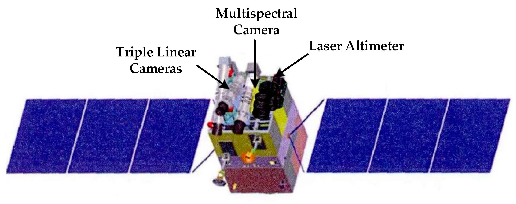
With the continuous improvement of China’s earth observation technology and the demand for large-scale stereo mapping, the idea of introducing geometric constraints provided by laser altimeter data to improve positioning accuracy has been put into practice. The recent Chinese ZY3-02 mission successfully produced 44 orbiter laser altimeter datasets. Subsequently, Tang et al. [25] and Xie et al. [26] built a rigorous geometric calibration model with pointing and ranging for correcting system errors of the laser altimeter onboard the ZY3-02 satellite, and this work realized high-precision in-orbit geometry calibration. It has been verified by Xie et al. [26] that the laser precision is about 2–3 m in areas with a slope less than 2°, and the absolute accuracy is better than 1 m in flat areas after calibration. Li et al. [27] performed experimental investigations of the integration of ZY3-02 satellite laser altimetry data and optical stereo images using combined adjustment by RFM with laser elevation constraint (RFM_EC) or RSM with laser ranging constraint (RSM_RC) with all result better than 3 m. However, there are two defects in their methods. On the one hand, the result obtained by RFM_EC is dependent on the laser altimeter data. On the other side, although the work also proposed the ranging constraint when using RSM, it failed to consider there exist attitude error for the altimeter because altimeter and stereo cameras are onboard the satellite.
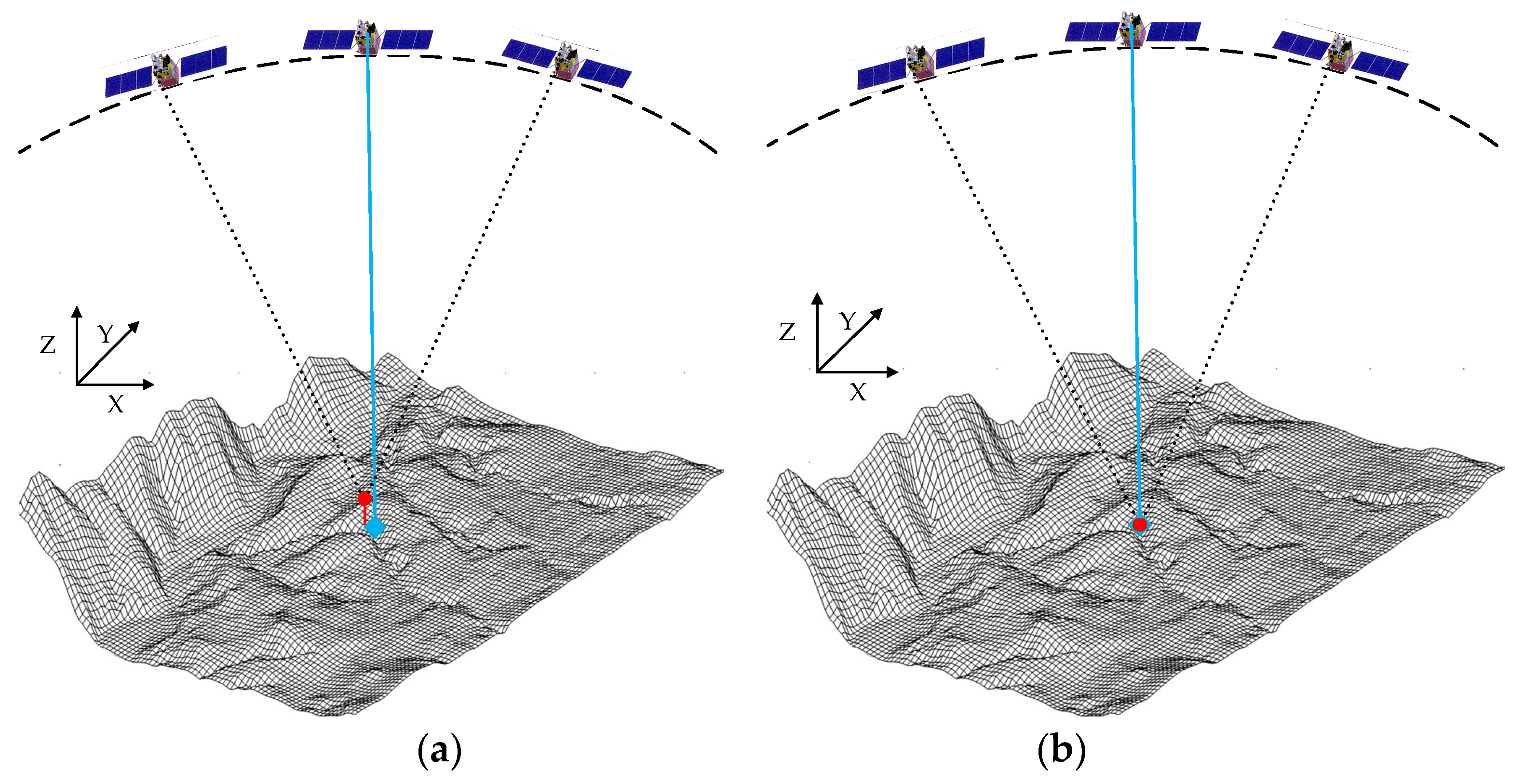
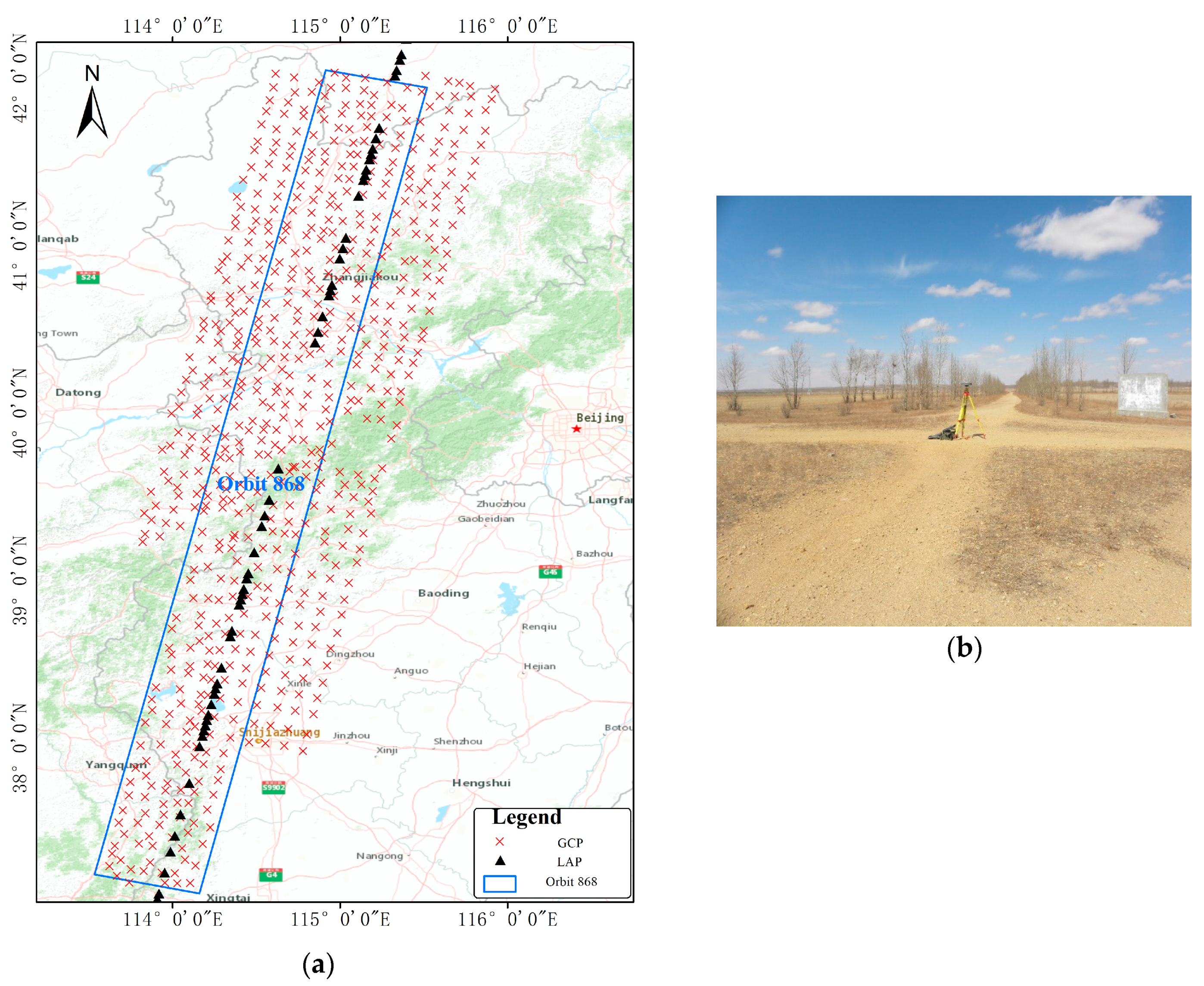
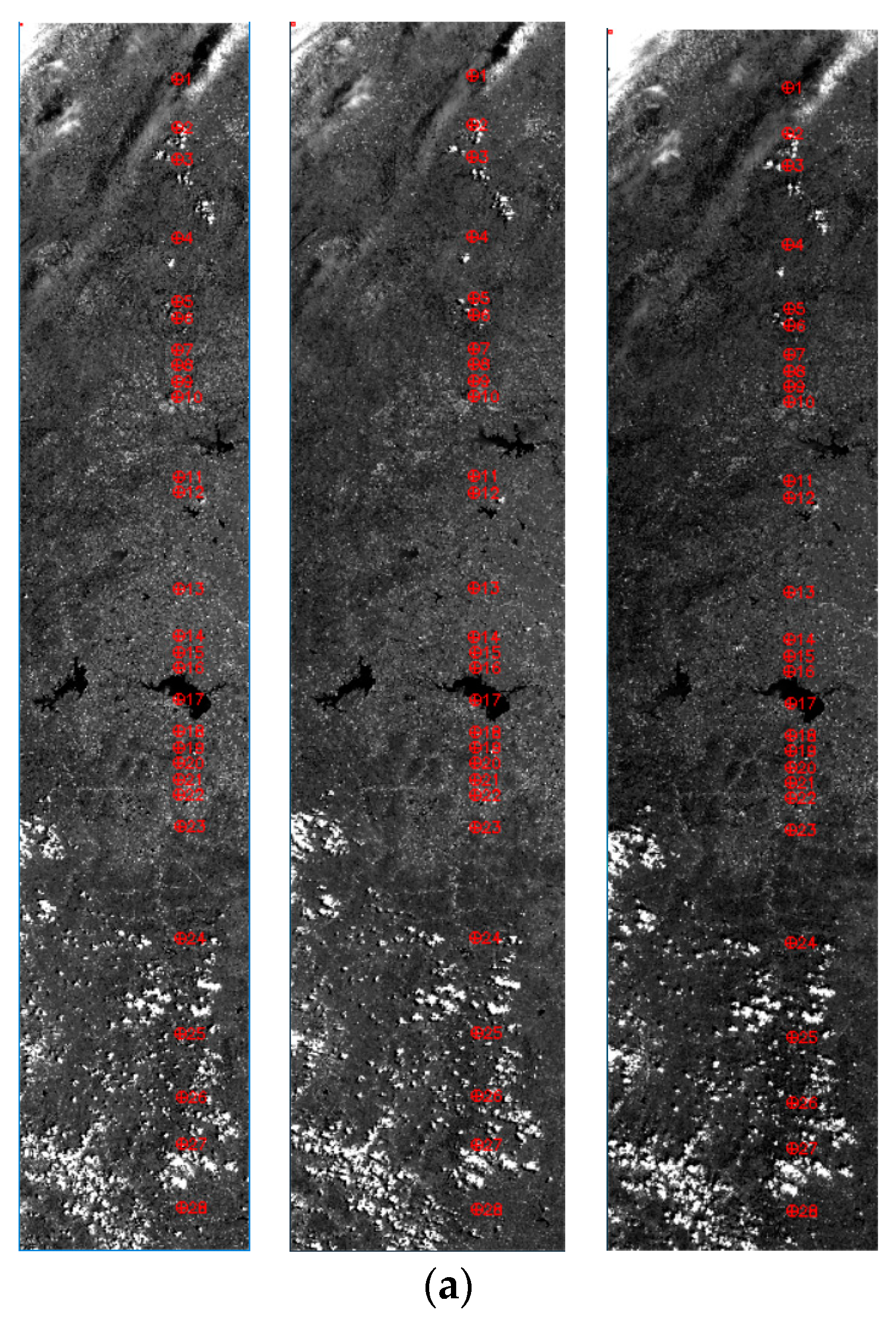
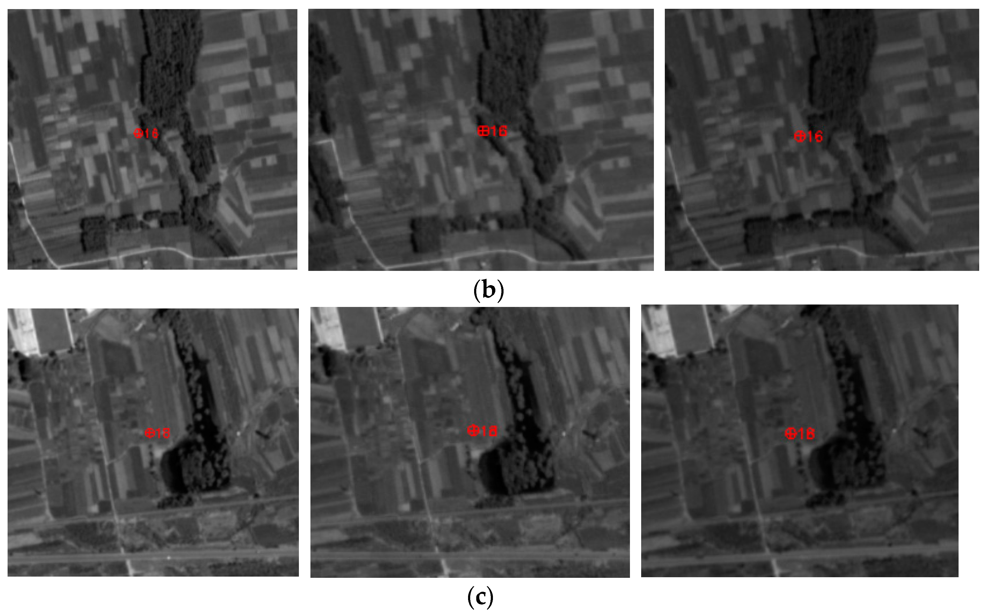
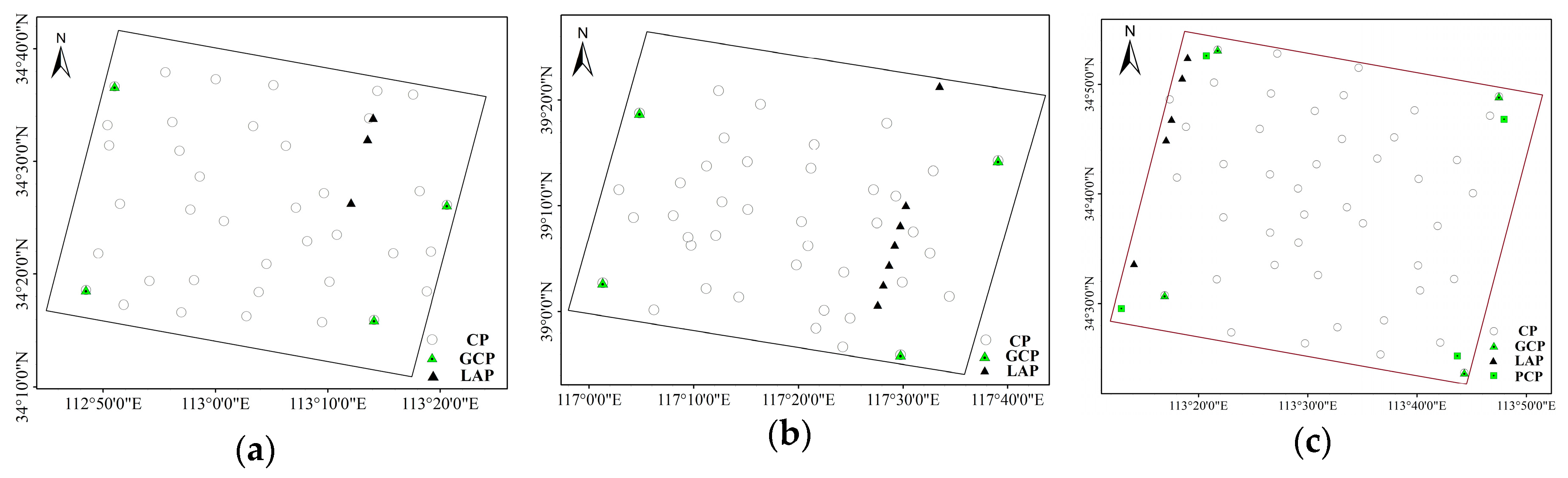
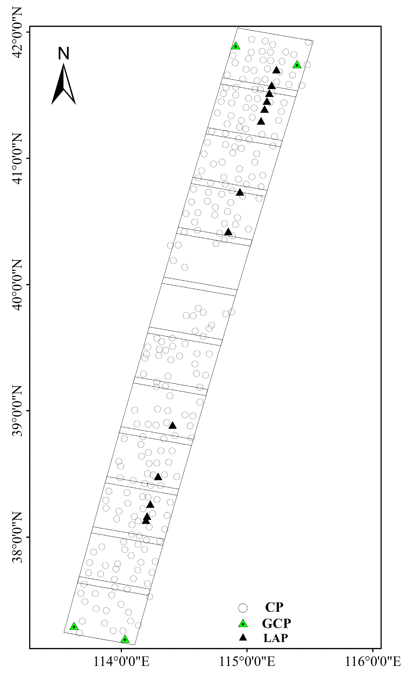
This paper presents an investigation into the integration of stereo imagery and laser altimeter data, which is achieved through combined adjustment with one constraint in image space so as to improve Earth topographic modeling. Compared with previous work, the proposed method highlights the following two aspects: (1) Laser ranging information is used as to improve the elevation accuracy of stereo images; (2) a constraint to minimize the back-projection discrepancies in image space is incorporated into the combined adjustment. Stereo images and laser altimeter data covering research areas in Songshan, Tianjin, Dengfeng, and Taihang were collected to conduct experiments, and a total of seven kinds of adjustment schemes were designed.

2. Materials and Methods

2.1. Specifications and Geometric Modeling of ZY3-02 Stereo Images and Laser Altimeter Data

2.1.1. Specifications of ZY3-02

Being the first operational surveying and mapping satellite for the development of China’s civil space infrastructure (CCSI) and the second satellite in the ZiYuan3 series [28], the ZY3-02 satellite was launched successfully on May 30, 2016 [29]. Phased 183° from each other and operating as a true constellation on the same orbit, the ZY3-01 and ZY3-02 constellation has enabled the revisit cycle to be shortened from 5 days to 3 days, which has increasingly improved the country’s ability to anticipate risks, managing crises effectively, and speed up the collection of data over large areas.
ZY3-02 is the first satellite equipped with an experimental laser altimeter for Earth observations in China. This configuration is mainly used to test the function and performance of the laser altimeter; it can be also used to explore the feasibility of obtaining high-precision elevation control data on Earth surface and the potential of using laser ranging data for increasing the precision of stereo mapping without using GCPs. In addition to the laser altimeter, other core payloads onboard the ZY3-02 include triple linear array cameras (TLCs), a multi-spectral camera, a dual-frequency Global Positioning System (GPS) receiver, star sensor, etc. For the ZY3-02, the orbit accuracy reaches the centimeter level and the attitude stability is approximately 5 × 10⁻⁴ °/s. A schematic diagram showing the installation of the laser altimeter and the TLCs is illustrated in Figure 1, wherein the pointing of the laser altimeter is substantially parallel to the visual axis of the nadir camera, with both pointing to the center of the Earth.
As illustrated in Figure 2, the TLCs onboard ZY3-02 are comprised of nadir-view (NAD), forward-view (FWD), and backward-view (BWD) linear CCD cameras, where the viewing angles of the FWD and BWD cameras are installed at an inclination of ±22° from the NAD to allow for the acquisition of stereo pairs along the flight direction. The number of CCDs in the FWD and BWD cameras focal plane has been decreased from four to three and the size has been changed from 10 μm to 7 μm with respect to the ZY3-01 satellite to enable ground resolution increases from 3.5 m to 2.7 m. The ground sample distance (GSD) for NAD imagery is still 2.1 m. For each camera among the TLCs, there are three CCDs with 8192 pixels per CCD and approximately 30 pixels between the overlapping areas of adjacent CCDs.
The laser altimeter onboard ZY3-02 is a test load and its main design parameters are shown in Table 1 [26,30]. Due to the limited mounting space, its volume is small and the function is relatively simple. Besides ranging, there is no echo waveform recording system and no laser footprint camera for the laser altimeter. In comparisons with ICESat/GLAS [4,5], it was found that the single-pulse laser energy emitted by the laser altimeter onboard ZY3-02 is about 200 mJ, which is higher than the 75 mJ of GLAS. Additionally, the ZY3-02 satellite is lower than GLAS in terms of the repetition frequency, while the designed ground size of the laser footprint spot is equivalent to that of GLAS. When the slope is less than 2°, the atmospheric transmittance is good, and when the surface reflectivity is high, the accuracy of laser ranging can be better than 1 m based on the geometric calibration and validation for the laser altimeter onboard ZY3-02 [26,30]. Although there is still a certain gap in comparison to the 0.1 m ranging accuracy level of GLAS, it appears promising to use these data to achieve ZY3-02 1:50,000 mapping without ground control points.

2.1.2. Geometric Model of TLCs

The construction of the laser altimeter and optical geometric imaging models formed the basis for the geometric positioning method and establishment of combined adjustment equations. Therefore, this section introduces the laser geometric imaging model, the optical geometric imaging model, and its inverse transformation model, which were used to construct the basic model needed for this research.
A typical rigorous geometric model for an optical linear camera is collinear equation [31,32], and hence, the geometric model for the TLCs hence was established as follows:
[ X Y Z ] W G S 84 = [ X G P S ( t ) Y G P S ( t ) Z G P S ( t ) ] W G S 84 + m R B o d y W G S 84 ( t ) [ x x 0 y y 0 f ] I
where [ X G P S ( t ) Y G P S ( t ) Z G P S ( t ) ] W G S 84 T are the coordinates of satellite in the World Geodetic System 1984 (WGS84), which are determined by precise orbit determination of ZY3-02 satellite [33]. R b o d y W G S 84 is the rotation matrix from the satellite body fixed coordinated system to WGS84. [ X G P S ( t ) Y G P S ( t ) Z G P S ( t ) ] W G S 84 T and R B o d y W G S 84 ( t ) together form the EO elements and both vary with scanning time t. [ x x 0 y y 0 f ] I T represent the direction of the light ray of a pixel in the satellite body fixed coordinate system, where I stands for the NAD/BWD/FWD camera. [ x 0 y 0 ] are the image coordinates of the principal point and f is the focal length; these form the interior orientation (IO) parameters. [ X Y Z ] W G S 84 T are the coordinates in WGS84 corresponding to the pixel, and m is a scale factor and an unknown.
It can be seen from the above Equation (1) above that the factors affecting the positioning accuracy are mainly the IO and EO parameters. The errors of IO parameters belong to the static error, and its errors can be accurately compensated after geometric calibration. In contrast, the errors of EO parameters including the measurement errors of the attitude and trajectory, will vary with time. To eliminate the errors caused by EO parameters, the offset matrix R u is used, in which the deviation between the real light ray and the uncorrected light ray is corrected [34,35]. Based on Equation (1), a corrected geometric model then can be reconstructed for the TLC of ZY3-02 as expressed in Equation (2):
[ X Y Z ] W G S 84 = [ X G P S ( t ) Y G P S ( t ) Z G P S ( t ) ] W G S 84 + m R b o d y W G S 84 ( t ) R u _ c a m I [ x x 0 y y 0 f ] I
R u _ c a m I is the offset matrix for corresponding camera I, and R b o d y W G S 84 ( t ) R u _ c a m I is defined as follows:
R b o d y W G S 84 ( t ) R u _ c a m I = [ a 1 a 2 a 3 b 1 b 2 b 3 c 1 c 2 c 3 ]
The above equation describes the calculation from image space to object space. For linear array camera, the inverse calculation from object space to image space can also be described as shown in Equation (4):
x = x 0 + f a 1 ( X G P S ( t ) X ) + b 1 ( Y G P S ( t ) Y ) + c 1 ( Z G P S ( t ) Z ) a 3 ( X G P S ( t ) X ) + b 3 ( Y G P S ( t ) Y ) + c 3 ( Z G P S ( t ) Z ) y = y 0 + f a 2 ( X G P S ( t ) X ) + b 2 ( Y G P S ( t ) Y ) + c 2 ( Z G P S ( t ) Z ) a 3 ( X G P S ( t ) X ) + b 3 ( Y G P S ( t ) Y ) + c 3 ( Z G P S ( t ) Z )
For convenience in the following derivations, the Equation (4) can be abbreviated as follows:
x = f c a m I _ x ( R u _ C a m I , X , Y , Z , I O c a m I , E O c a m I ) y = f c a m I _ y ( R u _ C a m I , X , Y , Z , I O c a m I , E O c a m I )

2.1.3. Geometric Model for the Laser Altimeter

A typical geometric model for laser altimeter is the range equation, which can be described as follows:
[ X l i d a r Y l i d a r Z l i d a r ] W G S 84 = [ X G P S ( t ) Y G P S ( t ) Z G P S ( t ) ] W G S 84 + ρ R b o d y W G S 84 ( t ) [ l x l y l z ]
where [ X G P S ( t ) Y G P S ( t ) Z G P S ( t ) ] W G S 84 T are the coordinates of satellite in WGS84 and R b o d y W G S 84 is the rotation matrix from the satellite body fixed coordinate system to WGS84. For the laser altimeter, [ X G P S ( t ) Y G P S ( t ) Z G P S ( t ) ] W G S 84 T and R b o d y W G S 84 are EO parameters and both vary with time; these values can be obtained by interpolation at any time t. [ l x l y l z ] T represent unit direction vector of the laser beam in the satellite body fixed coordinate system, where l x 2 + l y 2 + l z 2 = 1 . ρ is the range measured by the laser altimeter. [ X l i d a r Y l i d a r Z l i d a r ] W G S 84 T are the coordinates of the laser ground point in WGS84.
After the geometric calibration of laser altimeter, the main factors affecting the positioning accuracy are the errors of EO parameters. Similarly, the offset matrix is applied to compensate the errors of EO parameters. Then, Equation (6) can be reconstructed as follows:
[ X l i d a r Y l i d a r Z l i d a r ] W G S 84 = [ X G P S ( t ) Y G P S ( t ) Z G P S ( t ) ] W G S 84 + ρ R b o d y W G S 84 ( t ) R u _ l i d a r [ l x l y l z ]
Equation (7) can be furtherly abbreviated as follows:
X l i d a r = F l i d a r X ( R u _ l i d a r , ρ , E O l i d a r ) Y l i d a r = F l i d a r Y ( R u _ l i d a r , ρ , E O l i d a r ) Z l i d a r = F l i d a r Z ( R u _ l i d a r , ρ , E O l i d a r )
where R u _ l i d a r strands for the offset matrix to compensate the errors for the errors of EO parameters for the laser altimeter. Equation (7) also can be modified as follows:
ρ = | R 1 u _ l i d a r R b o d y W G S 84 ( t ) 1 ( [ X l i d a r Y l i d a r Z l i d a r ] [ X G P S ( t ) Y G P S ( t ) Z G P S ( t ) ] ) |
The Equation (9) is the constraint of laser ranging parameter. Similarly, for convenience in following derivations, the Equation (9) is abbreviated as:
ρ = | f l i d a r ( R u _ l i d a r , X l i d a r , Y l i d a r , Z l i d a r , E O l i d a r ) |

2.2. Integration of Stereo Images and Laser Altimeter Data for ZY3-02 Satellite

2.2.1. Overview of the Approach

A combined adjustment model with one constraint in image space is proposed for integrating the stereo images and laser ranging data of the ZY3-02 satellite. The block adjustment is constructed based on the principle of the intersection of corresponding light rays in the overlap region between stereo images. On the basis of the block adjustment model, the laser ranging information is introduced to form a combined adjustment model.
Given that the ZY3-02 experiment dataset used in this paper was level-0 data, the rigorous geometric positioning model for stereo cameras and laser altimeter data was built based on the Section 2.1 equations with initial IO and EO parameters. When the combined adjustment is employed, the initial EO parameters of the stereo images and laser altimeter data, the image coordinates, and the ground coordinates of stereo images’ tie points represent the main adjustment observations. The initial EO parameters can be obtained directly from the ZY3-02 level-0 data. The image coordinate observations are divided into the following two types: the tie points of stereo images and the image point coordinates of laser ground points. The stereo image tie points are the conjugate points of stereo images obtained by image registration. By applying the geometric model established by corresponding IO parameters and initial EO parameters, the image coordinates of laser ground points onto stereo images can be derived through the back-projection. There is an image space constraint when calculating the adjustment parameters in the combined adjustment for confining the process of adjustment. With the adjustment parameters, which mainly include the improved EO parameters, i.e., the offset matrix R u , and with the improved ground coordinates of laser points as final outputs, the improved geo-positioning accuracy of Earth topographic models can be achieved. The proposed approach can be summarized as follows:
(1)
Based on the initial orientation parameters, the geometric models of stereo images and laser altimeter data are built respectively;
(2)
Obtain the tie points of stereo images by image registration and their ground coordinates through space intersection;
(3)
Calculate the ground coordinates of LAPs and obtain the corresponding image coordinates in stereo images by back-projection; by using the laser points projected on the NAD camera image as references, obtain the LAPs on the BWD and FWD camera images by registration; the discrepancies between these two image coordinates are defined as the constraint in the combined adjustment;
(4)
Establish the observation equations for the combined adjustment model with the constraint in image space and solve the adjustment parameters;
(5)
Iterate steps (2)–(4) until the residuals of the adjustment parameters meet the threshold;
(6)
Generate the improved topographical model with the refined image orientation parameters and laser ground points.

2.2.2. Constraints in the Combined Adjustment Model

During the process of combing observation collected by stereo cameras and laser altimeter, because of the existence of various errors, e.g., attitude error, hardware errors, time synchronization errors, errors caused by changes in the space thermal environment, there might be discrepancies between the calculated and true values. In particular, the calculated laser ground points may differ from their real locations. Also, the calculated ground coordinates of tie points through space intersection may deviate from their true locations. Moreover, the back-projected laser ground points on stereo images may not be conjugate points and represent the different textural feature. These deviations reflect the inconsistency between stereo images and laser altimeter data by which we can establish the constraint equations, thus achieving the combined adjustment for ZY3-02 stereo images and laser altimeter data.
The key of combined adjustment is to take advantage of the high precision of laser ranging data, thereby confining the accuracy along the vertical direction in stereoscopic mapping. Figure 3 presents a schematic diagram showing the geometric relationship before and after the combined adjustment. In Figure 3, the light rays emitted by the FWD and BWD cameras are black dotted lines, and the laser light is a blue solid line. With respect to the laser altimeter, FWD and BWD cameras shoot the same ground point sequentially. It can be seen from Figure 3a that for the same ground point (black grid point in the figure), the elevation calculated by stereo images and the elevation measured by the laser altimeter are obviously inconsistent. Thanks to the high precision of the orbit and laser range, this combination provides a reliable measurement in the reference coordinate system along the vertical direction. Subsequently, the inconsistency between stereo images and laser altimeter data can be used to establish the range constraint of the combined adjustment, which is realized by minimizing discrepancies in image space, and the corrected intersection point is obtained. As shown in Figure 3b, the elevation calculated by stereo images’ space intersection is consistent to that of the LAP after combined adjustment, which improves the elevation accuracy of the stereo mapping and lays a foundation for high-precision stereo mapping.
The above range constraint is from the perspective in object space. Reversely, the range constraint can be analyzed in image space. Due to inaccurate EO parameters and inconsistencies between stereo images and laser altimeter data, the back-projected image coordinates on stereo images for the same laser ground point are not necessarily the true conjugate points. The issue is just to be solved in the combined adjustment.
In the case of a laser footprint camera onboard the satellite, the image point of laser footprint camera corresponding to the laser ground point can be directly extracted from the laser footprint image, and then, the accurate homologous points of the stereo camera for the laser ground point can be further obtained by matching the laser footprint image with stereo images using a high-precision matching method; however, this is not feasible for ZY3-02 because it is not equipped with a footprint camera. Nevertheless, according to the ZY3-02 satellite designer, the NAD camera and the laser altimeter can simultaneously work together. Moreover, the installation angles of the them are approximately identical with a deviation angle 0.92° [25,36]. Therefore, the image coordinates for the NAD camera derived by back-projecting the laser ground point can be seen as the intended position of the laser ground point to a large extent. As shown in Figure 4, the red image points on stereo images were obtained by back-projecting the blue laser ground point, and the green image points for the FWD and BWD cameras were obtained by high-precision matching with respect to the back-projected image point for the NAD camera. Theoretically, the discrepancies between the back-projected image points’ coordinates and matched image points’ coordinates should be zero for the FWD and BWD cameras, which is the basic idea of image space constraints that minimize the discrepancies in image space.

2.2.3. Combined Adjustment Model

The observation equation system for the combined adjustment of the ZY3-02 stereo images and laser altimeter data can be described in matrix form as follows:
v 1 = A x 1 + B x 2 l 1 P 1 v 2 = A x 1 + B x 3 l 2 P 2 v 3 = C x 3 + D x 4 l 3 P 3 v 4 = E x 5 l 4 P 4
There are four types of observation equations in the above equation. The first and second observation equations are related to the image tie points and the back-projected image coordinates of the laser ground point on the stereo images. The third is the laser range constraint observation equation, and the fourth is the additional constraint equation in the image plane. Here, x1 is the vector of the stereo cameras’ offset matrixes’ corrections, x2 is the vector of corrections to the ground coordinates of the tie points, x3 is the vector of corrections to the laser ground point, x4 is the vector of corrections to the laser altimeter’s offset matrix, and x5 actually includes x1, x3, and x4. A, B, C, D, and E are the partial derivations corresponding to the unknown parameters, and l is the constant term of the error equation. The weight Pi (i = 1, 2, 3, 4) in Equation (11) represents the contribution of each type of observation and can weaken the influence of the gross error in the adjustment system to a certain extent. Normally, weight parameter Pi is used with 10 times of a priori standard deviation σ i for each type of observation, and then, recalculate the weights Pi of each observations after each iterative adjustment.
The first kind of observation equation is actually the classic block adjustment model for tie points identified from stereo images. After linearization of Equation (5), which describes the relationship between the image point and ground point, the concrete expression for the first observation equation is established as follows:
v x _ I = f c a m I _ x R u _ c a m I d R u _ c a m I + f c a m I _ x ( X , Y , Z ) d ( X , Y , Z ) + f c a m I _ x ( R u _ c a m I 0 , X 0 , Y 0 , Z 0 , I O c a m I , E O c a m I ) x I v y _ I = f c a m I _ y R u _ c a m I d R u _ c a m I + f c a m I _ y ( X , Y , Z ) d ( X , Y , Z ) + f c a m I _ y ( R u _ c a m I 0 , X 0 , Y 0 , Z 0 , I O c a m I , E O c a m I ) y I
where the first and second coefficients represent the partial derivative of Equation (5) with respect to the offset matrix R u _ c a m I and the ground point coordinates ( X , Y , Z ) corresponding to A and B in Equation (11), respectively. d R u _ c a m I  and d ( X , Y , Z ) are corresponding to x1 and x2 in Equation (11) respectively. f c a m I _ x ( R u _ c a m I 0 , X 0 , Y 0 , Z 0 , I O c a m I , E O c a m I ) x I and f c a m I _ y ( R u _ c a m I 0 , X 0 , Y 0 , Z 0 , I O c a m I , E O c a m I ) y I are the constant terms corresponding to the term l1. ( X 0 , Y 0 , Z 0 ) represent the initial ground point coordinates of the image tie point determined by space intersection based on the initial values of the offset matrix R u _ c a m I 0 , initial stereo images’ IO and EO parameters.
The second kind of observation equation is very similar with the first, but here the image points are derived by the back-projection of laser ground points on stereo images and they are possibly not conjugate points because of existing various errors, which can be corrected by the process of combined adjustment. Similarly, the concrete expression of the second observation equation is established as follows:
v x _ I = f c a m I _ x R u _ c a m I d R u _ c a m I + f c a m I _ x ( X l i d a r , Y l i d a r , Z l i d a r ) d ( X l i d a r , Y l i d a r , Z l i d a r ) + f c a m I _ x ( R c a m I 0 , X l i d a r 0 , Y l i d a r 0 , Z l i d a r 0 , I O c a m I , E O c a m I ) x I v y _ I = f c a m I _ y R u _ c a m I d R u _ c a m I + f c a m I _ y ( X l i d a r , Y l i d a r , Z l i d a r ) d ( X l i d a r , Y l i d a r , Z l i d a r ) + f c a m I _ y ( R c a m I 0 , X l i d a r 0 , Y l i d a r 0 , Z l i d a r 0 , I O c a m I , E O c a m I ) y I
where the definitions of the first and second coefficients in Equation (13) are same as those in Equation (12). d R u _ c a m I and d ( X l i d a r , Y l i d a r , Z l i d a r ) corresponding to x1 and x3 in Equation (11), respectively. f c a m I _ x ( R c a m I 0 , X l i d a r 0 , Y l i d a r 0 , Z l i d a r 0 , I O c a m I , E O c a m I ) x I and f c a m I _ y ( R c a m I 0 , X l i d a r 0 , Y l i d a r 0 , Z l i d a r 0 , I O c a m I , E O c a m I ) y I are the constant terms corresponding to the term l2. ( X l i d a r _ 0 , Y l i d a r _ 0 , Z l i d a r _ 0 ) represent the initial coordinates of laser ground point which are obtained based on the geometric model for the laser altimeter in Equation (10) by using the range, initial offset matrix R u _ l i d a r 0 and EO parameters.
The third kind of observation equation is a modification of Equation (10) constrained by the laser range as follows:
F d ρ = ρ | f l i d a r ( R u _ l i d a r , X l i d a r , Y l i d a r , Z l i d a r , E O l i d a r ) | = 0
After linearization, the concrete expression of the second observation equation is established as follows:
V F d ρ = F R u _ l i d a r d R u _ l i d a r + F ( X l i d a r , Y l i d a r , Z l i d a r ) d ( X l i d a r , Y l i d a r , Z l i d a r ) + ρ f l i d a r ( R u _ l i d a r 0 , X l i d a r 0 , Y l i d a r 0 , Z l i d a r 0 , E O l i d a r )
where the first and second coefficients represent the partial derivative of Equation (14) with respect to offset matrix R u _ l i d a r and the laser ground point coordinates ( X l i d a r , Y l i d a r , Z l i d a r ) corresponding to C and D in Equation (11) respectively. d R u _ l i d a r and d ( X l i d a r , Y l i d a r , Z l i d a r ) correspond to x3 and x4 in Equation (11) respectively.
ρ f l i d a r ( R u _ l i d a r 0 , X l i d a r 0 , Y l i d a r 0 , Z l i d a r 0 , E O l i d a r ) are the constant terms corresponding to the term l3 and R u _ l i d a r 0 is the initial values of the offset matrix for the laser altimeter.
The fourth kind of observation equation is the image space constraints which can be represented as follows:
F d x = x b a c k p r o j e c t e d _ F W D / B W D x m a t c h _ F W D / B W D = 0 F d y = y b a c k p r o j e c t e d _ F W D / B W D y m a t c h _ F W D / B W D = 0
where x b a c k p r o j e c t e d _ F W D / B W D and y b a c k p r o j e c t e d _ F W D / B W D are the image points’ coordinates of the back-projected laser ground points on FWD and BWD cameras and are used as adjustment parameters. x m a t c h _ F W D / B W D and y m a t c h _ F W D / B W D are the matched image points’ coordinates with respect to the back-projected image point on NAD camera and are used as constants. Based on Equations (5) and (8), the concrete expression of the fourth kind of observation equation is established as follows:
V F d x = f F W D / B W D _ x ( R u _ F W D / B W D , X l i d a r , Y l i d a r , Z l i d a r ) R u _ F W D / B W D d R u _ F W D / B W D + f F W D / B W D _ x ( R u _ F W D / B W D , X l i d a r , Y l i d a r , Z l i d a r ) X l i d a r R F l i d a r X R u _ l i d a r d R u _ l i d a r + f F W D / B W D _ x ( R u _ F W D / B W D , X l i d a r , Y l i d a r , Z l i d a r ) Y l i d a r R F l i d a r Y R u _ l i d a r d R u _ l i d a r + f F W D / B W D _ x ( R u _ F W D / B W D , X l i d a r , Y l i d a r , Z l i d a r ) Z l i d a r R F l i d a r Z R u _ l i d a r d R u _ l i d a r + f F W D / B W D _ x ( R u _ F W D / B W D 0 , X l i d a r 0 , Y l i d a r 0 , Z l i d a r 0 ) x m a t c h _ F W D / B W D V F d y = f F W D / B W D _ y ( R u _ F W D / B W D , X l i d a r , Y l i d a r , Z l i d a r ) R u _ F W D / B W D d R u _ F W D / B W D + f F W D / B W D _ y ( R u _ F W D / B W D , X l i d a r , Y l i d a r , Z l i d a r ) X l i d a r R F l i d a r X R u _ l i d a r d R u _ l i d a r + f F W D / B W D _ y ( R u _ F W D / B W D , X l i d a r , Y l i d a r , Z l i d a r ) Y l i d a r R F l i d a r Y R u _ l i d a r d R u _ l i d a r + f F W D / B W D _ y ( R u _ F W D / B W D , X l i d a r , Y l i d a r , Z l i d a r ) Z l i d a r R F l i d a r Z R u _ l i d a r d R u _ l i d a r + f F W D / B W D _ y ( R u _ F W D / B W D 0 , X l i d a r 0 , Y l i d a r 0 , Z l i d a r 0 ) x m a t c h _ F W D / B W D
where the first four coefficients correspond to x5 in Equation (11) which is the partial derivative of Equation (5) with respect to the offset matrix and of Equation (8) with respect to the laser ground point. It should be noted that the R u _ l i d a r is same with R u _ N A D in Equations (12) and (13).

2.3. Introduction to the Experimental Area and Data Sources

To sufficiently validate the proposed integration model, ZY3-02 stereo images and laser altimeter data covering the Songshan, Taihang, Dengfeng, and Tianjin areas in China were collected. The Songshan, Dengfeng, and Tianjing datasets consisted of only one standard scene and associated laser altimeter data, where each standard scene included NAD, BWD, and FWD stereo images. The Songshan and Dengfeng research areas are mountainous areas with complex topography, while the Tianjin research area is located in the plain area. As shown in Figure 5a, the Taihang dataset consisted of one strip of scenes (12 standard scenes) and one strip of laser altimeter data (orbit 944). This dataset crossed the Taihang Mountains and covered a total area of around 55 km × 550 km; the height range varied from 75 to 2,750 m. The topography of the Taihang dataset was varied and complex, encompassing mountains, basins, hills, and plains. General information about the experimental data is listed in Table 2, where the location stands for the location of the laser altimeter in relation to stereo images. There were two location groups to verify the influence of the location of the laser altimeter in relation to stereo images on the results of the combined adjustment. It should be noted that the stereo images and laser altimeter data were not acquired simultaneously. Ideally, the acquisition time should be the same so that the image coordinates obtained by back projecting the LAPs on NAD camera imagery can be more consistent with the true value. However, because of the acquisition time interval between the stereo images and laser altimeter data was relatively short and the pointing angle between them was consistent, the error induced by the non-simultaneous acquisition could be neglected.
With the final output based on the improved EO parameters and improved ground coordinates of laser points, improved geo-positioning accuracy of Earth topographic models can be achieved. Therefore, the experiments were mainly used to verify the more intuitive geo-positioning accuracy by using check points (CPs). The CPs for the Songshan, Taihang, and Dengfeng research areas were manually extracted from a 1:5000 digital orthophoto map/digital elevation model (DOM/DEM) of Songshan, 1:2000 DOM/DEM of Dengfeng, and 1:2000 DOM/DEM of Tianjin, for which specific information is given in Table 3. For Taihang, there were 621 GCPs available to check the performance of the combined processing technique. The WGS84 coordinates of the GCPs were determined by static GPS processing and with accuracies exceeding 0.1 m; most of them were located in road intersections and manually picked its’ corresponding image point coordinates (x,y). Besides, four plane control points (PCPs), i.e., ground points with only known plane coordinates and unknown heights, were used. Figure 5b presents a detailed view of a GCP in the field.
It should be noted, that invalid laser altimeter data existed because of the influence of the atmosphere, vegetation, complex terrain, and other factors, so not all of the original laser altimeter data were used in the combined adjustment. For the laser altimeter of the ZY3-02 satellite, because it has no full waveform recording function, only ranging information and relatively simple ranging attributes such as echo detection anomalies, transmission anomalies, and other basic parameters, invalid LAPs could only be filtered out according to the basic ranging parameters. Then, ground coordinates of laser footprint points were calculated and invalid laser points within the existing terrain reference data were eliminated, such as those within the Shuttle Radar Topography Mission (SRTM) data. Invalid laser points were eliminated by following steps:
1.
Calculate the ground coordinates ( X l i d a r , Y l i d a r , Z l i d a r ) in the geocentric Cartesian coordinate system for laser footprint based on the geometric model of laser altimeter, and convert the coordinates ( X l i d a r , Y l i d a r , Z l i d a r ) in the geocentric Cartesian coordinate system to the coordinates ( L a t l i d a r , L o n l i d a r , H l i d a r ) in the geographical coordinate system;
2.
Second, extract the elevation value H S R T M that can be directly interpolated in SRTM data according to the plane coordinates ( L a t l i d a r , L o n l i d a r ) of the laser footprint. It is noted that the H S R T M should be converted to the same height Datum with the elevation H l i d a r ;
3.
Compare elevation of the laser footprint H l i d a r with the elevation value of SRTM H l i d a r to calculate the δ h , and eliminate the laser points satisfying the condition δ h > 3 σ , σ is the absolute elevation accuracy of SRTM data.
Besides, some plane control points (PCPs) in Dengfeng area were manually extracted from YG-13 SAR image. For the PCP, its plane coordinates in object space are known while the height coordinate is unknown. The plane accuracy of PCPs was within 1.5 m [37] and Figure 6 illustrates a detail view of PCP.

3. Results

3.1. Inconsistency between ZY3-02 Stereo Camera Images and Laser Ranging Data

Using the initial orientation parameters of ZY3-02 stereo camera images and laser altimeter, the geometric model of them can be established. Then, the ZY3-02 LAP can be overlaid on the stereo images by back-projecting the LAPs directly. Figure 7 shows the ZY3-02 stereo images and corresponding laser altimeter data at the Taihang research area. Figure 7a shows the planar view of the laser altimeter data overlaid on the stereo images, where the left image shows the NAD, the center one shows BWD and the right shows the FWD image. The distance between adjacent laser footprints in NAD camera image is almost 1706 pixels, whose corresponding distance of ground laser spot is about 3.4 km. Due to the existence of invalid laser data which has been eliminated between the laser footprints, the distance between some of the individual laser footprint is several times of 1706 pixels. For example, the distance between laser points 1 and 2 on the NAD image is about 5118 pixels, with two invalid data in the middle.
For the same LAPs overlaid on the NAD, BWD, FWD images, the image points on three-view images are not the homologous points which represent the same textural feature as shown in Figure 7b. The range calculated by stereo images’ space intersection is not conform with the laser range. Using the laser points projected on the NAD camera image as references, the LAPs on the BWD and FWD camera images can be obtained by registration which named matched image points. After making the statistics of discrepancies between the back-projected image points’ coordinates and matched image points’ coordinates for BWD and FWD images respectively, it can be found that for BWD image, the Root Mean Square Error (RMSE) are 2.7 pixels across track and 2.0 pixels along track respectively, for FWD image, the RMSE are 3.1 pixels across track and 2.9 pixels along track respectively. This shows that inconsistency between stereo images and laser altimeter data exists. The main error sources are the orientation parameters. The proposed combined adjustment is to utilize the laser range with high accuracy for correcting the orientation parameters and elimination of these inconsistencies.

3.2. Validation of the Proposed Combined Adjustment Model

3.2.1. Validation Using the Standard Scene

In the Songshan, Dengfeng, and Tianjin research areas, there were evenly distributed GCPs that were manually extracted from the DOMs and DEMs. These GCPs served as CPs to validate the accuracy of the combined adjustment. Considering that the picking accuracy was limited by the blur effect [38], the final accuracy of CPs was approximately within 1 m. As mentioned above, not all of the laser altimeter data were used in the combined adjustment because of the existence of invalid data. Given that the ranging accuracy of the laser altimeter of ZY3-02 can be better than 1.0 m when the slope is less than 2° and the laser footprint size is about 75 m, all of the laser altimeter data used in the experiment were prescreened by using DEM data and most of the data used were located in the plain area. Five types of adjustment experiments were carried out, and the specific plans of the experiments were designed as follows:
1.
Plan 1: the free-net block adjustment without GCPs;
2.
Plan 2: block adjustment with four GCPs distributed at four corners of the research area;
3.
Plan 3: proposed combined adjustment using one LAP located in the middle of the research area;
4.
Plan 4: proposed combined adjustment using two LAPs located in the middle and start or end of the research area;
5.
Plan 5: proposed combined adjustment using all of the available LAPs in the research area.
In addition to the five types of adjustment experiment, another two type were designed for attempting to improve the plane accuracy in the combined adjustment.
6.
Plan 6: proposed combined adjustment using the additional PCPs in the research area;
7.
Plan 7: proposed combined adjustment using all of the available LAPs and the additional PCPs simultaneously in the research area.
Specifically, for the image tie points with known PCPs, its plane coordinates (X,Y) in object space did not participate in the adjustment and were deemed constants ( X P C P , Y P C P ) . Only the height value of the tie points with known PCPs is to be solved. This can be accomplished with the following modified version of Equation (12):
v x _ I = f c a m I _ x R u _ c a m I d R u _ c a m I + f c a m I _ x ( Z ) d ( Z ) + f c a m I _ x ( R u _ c a m I 0 , X P C P , Y P C P , Z 0 , I O c a m I , E O c a m I ) x I v y _ I = f c a m I _ y R u _ c a m I d R u _ c a m I + f c a m I _ y ( Z ) d ( Z ) + f c a m I _ y ( R u _ c a m I 0 , X P C P , Y P C P , Z 0 , I O c a m I , E O c a m I ) y I
Figure 8 shows the points’ (CPs, GCPs, LAPs, PCPs) distribution in the Songshan, Dengfeng, and Tianjin area.
As shown in Table 4, the height accuracy in the research areas improved significantly after integration with the laser altimeter data by using the proposed combined adjustment. In Songshan, for example, the height accuracy improved from 16.73 m to 3.79 m by using one LAP, which was equivalent to that obtained from block adjustment with four GCPs, thus demonstrating the effectiveness of the proposed combined adjustment of ZY3-02 stereo images and laser altimeter data. Besides, the improved height accuracy was found to be insensitive to the number of LAPs and the location with respect to stereo images. On the one hand, when different numbers of laser points were used in the combined adjustment, the results improved almost to the same extent and even one LAP achieved good results. However, it is worthwhile to mention that all of the available LAPs in the research area were involved in the processing of the combined adjustment for the results with high reliability. On the other hand, the location of laser altimeter data on the stereo images was on the left side for Tianjin and in the center–right side for the other areas, but the final results revealed that the relative position had little effect on the improved efficiency.
Moreover, when both PCPs and LAPs were used, it can improve the plane and elevation accuracy at the same time, which is slightly lower than the results of block adjustment with four GCPs. This is because the solutions of combined adjustment are constrained by the known PCPs. After PCPs were allowed to participate in the proposed combined adjustment, the method was found to be promising for improving the plane and elevation accuracy simultaneously, and thus, additional improvements in topographical modeling could be achieved. However, it should be noted that the PCPs were directly used as constants rather than as adjustment parameters, which means that the results for the planimetric accuracy will be decided by the accuracy of the PCPs.
To further quantitatively assess the performance of the approach, two DEMs in Dengfeng were generated based on the P6 and P7 combined adjustment results respectively. The Semi-Global Matching (SGM) method [39] was introduced to acquire the point cloud, and then, the digital surface model (DSM) at a 5 m sampling distance was directly generated from the point cloud. The corresponding reference DEM in Dengfeng was used, and detailed information about Dengfeng is listed in Table 3. The generated DEM was tested for different terrains such as mountainous, hilly and flat plain areas to comprehensively evaluate the DEM quality. As show in Table 5, the results indicate that the participation of laser altimeter data can bring promising height accuracy.
As it can be seen in Figure 9a, in that the DEM is generated from the P6, there obviously exists a systematic error in the elevation difference resulted from where the terrain can even be observed. Figure 9b shows the DEM elevation difference using P7. The elevations are generally in line with the reference DEM. It can be noticed that there are places like black holes, which represent the larger elevation difference whatever in Figure 9a or in Figure 9b. The reference DEM used in the experiment were obtained in 2012 year, while the generated DEM were obtained in 2016 year. These mining areas were exploited after 2012 year. When making statistics of the difference, the difference in mining areas hence influence the result and cause large difference finally. Generally, the proposed combined adjustment can effectively improve the elevation accuracy.

3.2.2. Validation at the TaiHang Area

Unlike in Songshan, Dengfeng and Tianjin, there were total 12 standard scenes covering Taihang. All of the CPs in the stereo images were manually extracted based on the GCPs in the Taihang area with distinct features and in the plain area, and the accuracy of CPs was approximately within 1 m because of the accuracy achieved with the manual selection and the blur effect. Similarly, only some screened LAPs were used in the processing of combined adjustment. The detail points’ distribution were illustrated in Figure 10.
Table 6 shows the statistics for the positioning accuracy under different adjustment schemes in the Taihang area. The plane (CE90) and elevation accuracy (LE90) were 4.13 m and 2.15 m, respectively, when using four GCPs around four corners. When LAPs were used in the proposed combined adjustment, the elevation accuracy improved significantly, with the height accuracy being improved from 10.51 m to 2.87 m when using 13 LAPs. As can be seen in Figure 11, the previous inconsistencies were removed after the combined adjustment. The projected points on the stereo images were the homologous points, and the discrepancies were reduced.

4. Discussion

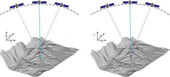
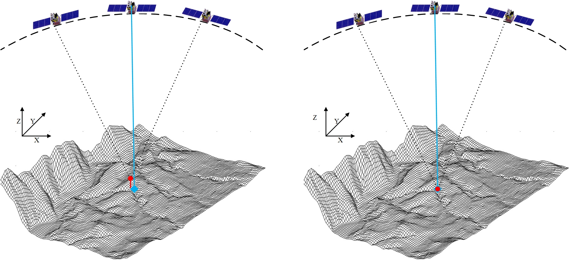
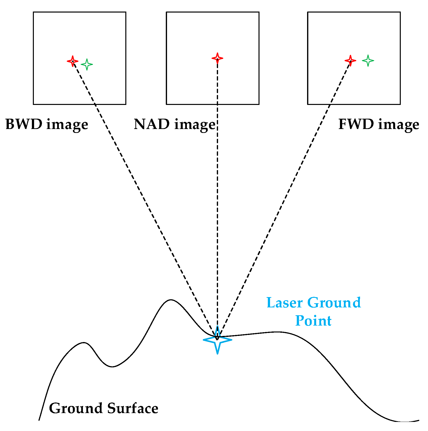
As mentioned previously, the image coordinates for the NAD camera derived by back-projecting the laser ground points can be treated as the intended position of laser ground points on the basis of the NAD camera and laser altimeter onboard ZY3-02 working together simultaneously and the installation angles of them being identical. However, the NAD camera images and corresponding laser altimeter data used in the experiments were captured at different times because simultaneously captured NAD images and laser altimeter data were unavailable due to satellite shooting schedule and limited data collection. Besides, due to the impact of the satellite launch and the physical environment changes in the orbit, the NAD camera and laser altimeter installation angles may slightly change. Therefore, the difference in the capture dates of the two datasets and the slightly different viewing angles could result in accuracy loss for the proposed combined adjustment, but the errors can be analyzed quantitatively. 
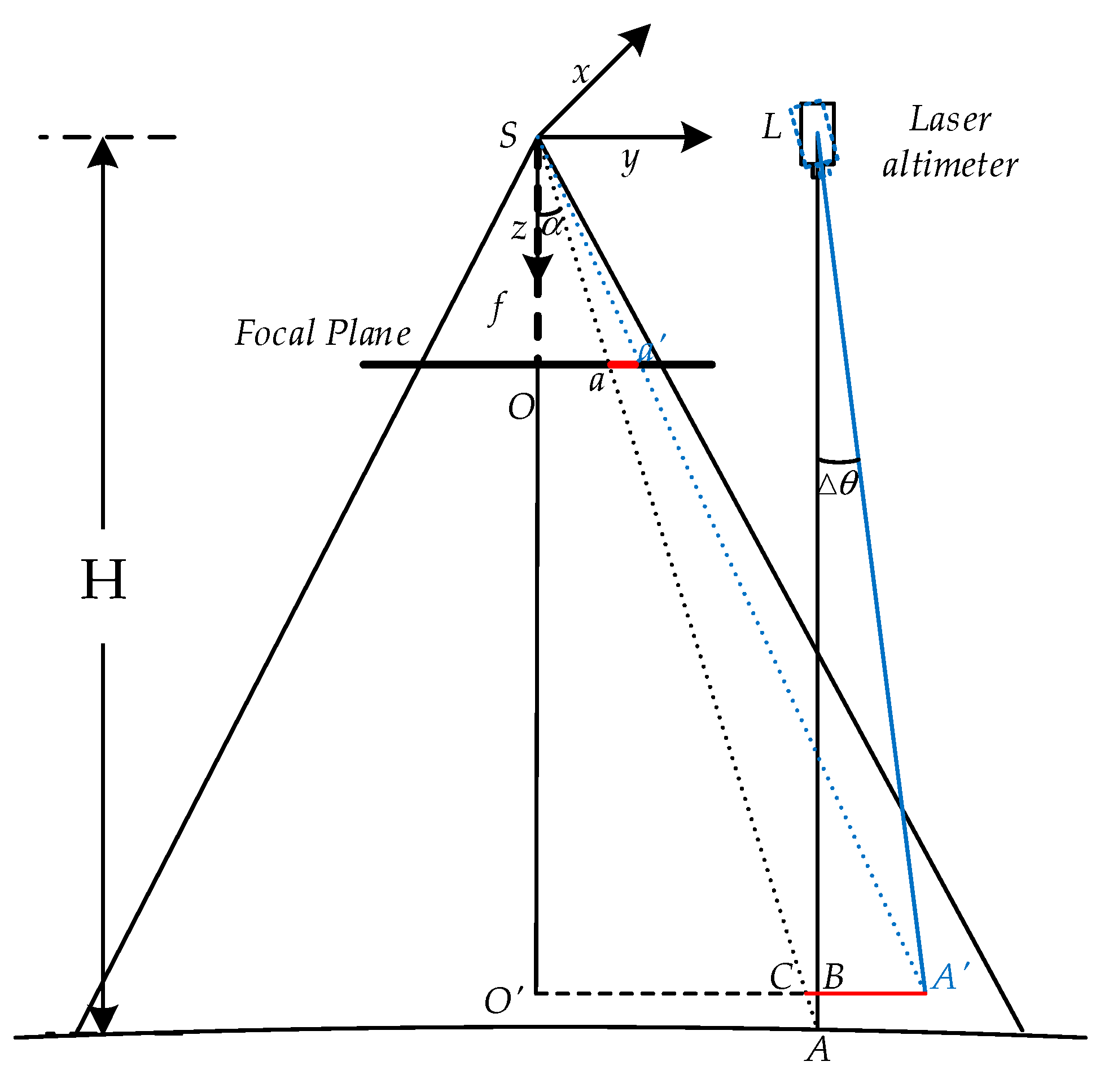
Figure 12 shows the elevation error analysis schematic.
S is the projected center of the NAD camera. The thick solid line represents the focal plane, and SO is the focal length f. The black laser altimeter represents an ideal situation, that it simultaneously works with the NAD camera, while the blue represents the real situation due to some unfavorable factors such as changes in the thermal environment and attitude stability, in which there exists a small deviation angle θ between the true and real pointing angles that ultimately may change and cause variations in the relative geometric relation of the NAD camera. To simplify the analysis, suppose there is θ only along the axis y. Here, only consider the factors outside the laser altimeter, so the difference of measured range between the ideal and true is zero. Laser point A projects to the NAD image at a, and laser point A’ projects to the NAD image at a’. The view angle a S O of image point a in the image coordinate is a. The relative location of LAP in relation to the image can result in different view angles α . Thus, aa’ is the projection error resulting from the capture time interval.
To calculate aa’, we draw a line over A’ parallel to aa’, which intersects LA at B, and SA at C. Then, the projection error aa’ can be calculated by:
a a = A C f S O = A C f H A B = ( H sin θ + H tan α ( 1 cos θ ) ) f H cos θ
Taking the derivative of Equation (19) with respect to, the derivative of aa’ is:
a a α = H ( 1 cos θ ) sec 2 α f H cos θ
Since the value of a a / α is always greater than 0, aa’ is a monotonically increasing function about variable α . Thus, the maximum value of α  at the end pixel of NAD camera image, aa’ is the maximum projection error.
Taking the derivative of Equation (19) with respect to θ , the derivative of aa’ is:
a a θ = ( H cos θ + H tan α ( 1 + sin θ ) ) f H cos θ + ( H sin θ + H tan α ( 1 cos θ ) ) f H sec θ tan θ
Since the value of a a / θ is also always greater than 0, a a is a monotonically increasing function about variable θ .
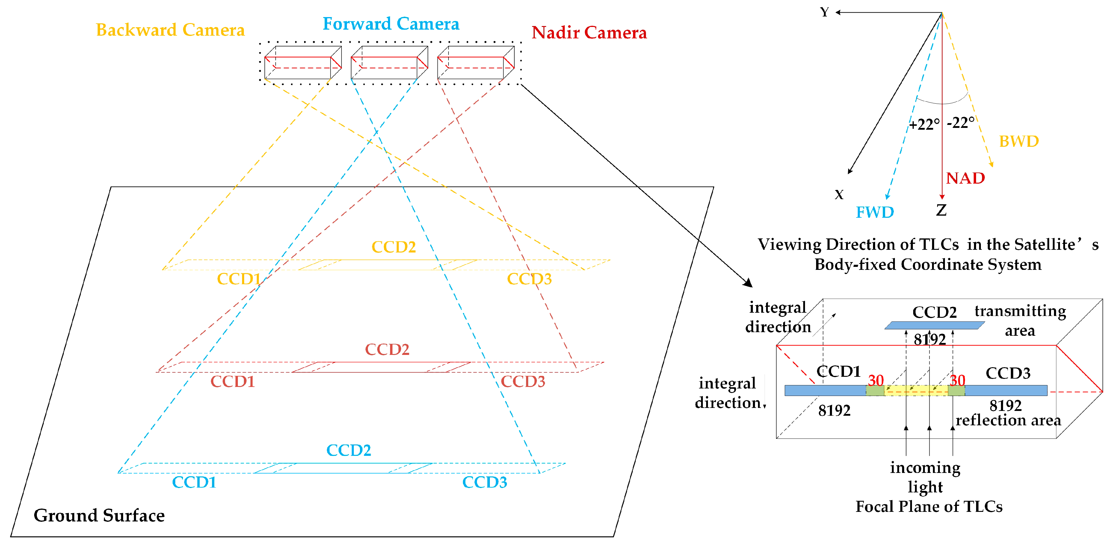
For the ZY3-02 satellite, f is 1.7 m, the NAD image pixel size is 7 µm, and the minimum and maximum view angles are 0° and 2.94°, respectively. Because the interval time is 5 days, suppose the maximum deviation θ is 5 within such a short interval. According to the calculation results, the value of aa’ is approximately 5.88 pixels in the image (12.35 m in ground space), whatever minimum or maximum view angle is used, which demonstrates that the combined adjustment results are insensitive to the location of the LAP in relation to the stereo images. Moreover, all of the LAPs engaged in the experiment were selected at the plain area with slopes of less than 2°. The 12.35 m deviation in the planimetric space will bring about a maximum 0.43 m error in the vertical direction when the slope is 2°. Overall, the error is relatively small compared with the original height accuracy acquired from stereo images of the ZY3-02 satellite. To eliminate the errors caused by capture time interval, the NAD image and laser altimeter data that are captured simultaneously remain the best choice to use for experiments.

5. Conclusions

In this study, a combined adjustment model with one constrain in image space was proposed for integration of ZY3-02 stereo images and laser altimeter data for improved Earth topographic modeling. This proposed approach takes advantage of the accurate laser range to improve the positioning accuracy of stereo images, especially the elevation accuracy. Stereo images and laser altimeter data in several areas were collected as experiment data for validation work. Several conclusions can be drawn from this research, and these are summarized below:
(1)
Inconsistencies exist between the stereo images and laser altimeter data for the ZY3-02 satellite. For the same LAP overlaid on the NAD, BWD, and FWD images, the image points on three-view images are not the homologous points, and this is mainly caused by the errors of orientation parameters. The proposed combined adjustment utilizes the laser range with high accuracy for correcting the orientation parameters and eliminating these inconsistencies.
(2)
After applying the proposed combined adjustment, a superior elevation accuracy can be achieved. Experiments demonstrated that the height accuracy can be improved significantly to the extent of that obtained from block adjustment with four GCPs. Validation work further proved that the improved height accuracy is insensitive to the number of LAPs and locations of LAPs in relation to stereo images. It is suggested that all of the available LAPs in the research area should be involved in the processing of the combined adjustment to obtain results with high reliability.
(3)
By introducing the additional PCPs engaged in the combined adjustment, the planimetric accuracy can be improved along with the elevation accuracy. In the Dengfeng area experiment, the adjustment results derived by using LAPs and additional four LAPs were slightly lower than the results from the block adjustment with four GCPs.
Despite the promising results achieved for integration of stereo images and laser altimeter data of ZY3-02, so far only the elevation accuracy can be improved. This study attempts to improve the planimetric accuracy simultaneously by integration with PCPs, which can be obtained from the results of other sensors. Nevertheless, the final results will be decided by the accuracy of PCPs. Thus, further research about integration with other sensors that can acquire reliable observations in planar space is required, rather than directly using the results. That is, integration of data from multi-sensors is an important topic for future studies.

Author Contributions

K.X., G.Z., and D.L. conceived and designed the experiments; K.X., G.Z. performed the experiments; K.X., P.J. and X.H. analyzed the data; K.X. wrote the paper.

Funding

This research was supported by the Key research and development program of the Ministry of Science and Technology (2018YFB0504905, 2016YFB0500801), Quality improvement of Chinese satellite data and comprehensive application demonstration of Geology and mineral resources, National Natural Science Foundation of China (Grant No. 41601490).

Acknowledgments

We give thanks to the research team at Satellite Surveying and Mapping Application Center, National Administration of Surveying Mapping and Geo-information for freely providing ZY3-02 data. Furthermore, the authors would like to thank the editors and the anonymous reviewers for their constructive comments.

Conflicts of Interest

The authors declare no conflict of interest.

References

  1. Tang, X.M.; Xie, J.F.; Wang, X.; Jiang, W.S. High-Precision Attitude Post-Processing and Initial Verification for the ZY-3 Satellite. Remote Sens. 2015, 7, 111–134. [Google Scholar] [CrossRef]
  2. Kubik, P.; Latry, C.; Lebegue, L. PLEIADES-HR 1A&1B image quality commissioning: Innovative radiometric calibration methods and results. In Proceedings of the SPIE 8866, Earth Observing Systems XVIII, San Diego, CA, USA, 23 September 2013; pp. 886610–886611. [Google Scholar]
  3. Bouillon, A.; Breton, E.; Lussy, F.D.; Gachet, R. SPOT5 geometric image quality. In Proceedings of the 2003 IEEE International Geoscience and Remote Sensing Symposium, IGARSS ′03, Toulouse, France, 21–25 July 2003; pp. 303–305. [Google Scholar]
  4. Abshire, J.B.; Sun, X.L.; Riris, H.; Sirota, M.; McGarry, J.; Palm, S.; Ketchum, E.A.; Follas, R.B. Geoscience laser altimeter system (GLAS) on the ICESat mission: Pre-launch and on-orbit measurement performance. In Proceedings of the IGARSS 2003, 2003 IEEE International Geoscience and Remote Sensing Symposium (IEEE Cat. No.03CH37477), Toulouse, France, 21–25 July 2003; pp. 1534–1536. [Google Scholar]
  5. Schutz, B.E.; Zwally, H.J.; Shuman, C.A.; Hancock, D.; DiMarzio, J.P. Overview of the ICESat Mission. Geophys. Res. Lett. 2005, 32. [Google Scholar] [CrossRef] [Green Version]
  6. Abshire, J.B.; Sun, X.L.; Afzal, R.S. Mars Orbiter Laser Altimeter: Receiver model and performance analysis. Appl. Opt. 2000, 39, 2449–2460. [Google Scholar] [CrossRef] [PubMed]
  7. Shan, J.; Yoon, J.S.; Lee, D.S.; Kirk, R.L.; Neumann, G.A.; Acton, C.H. Photogrammetric Analysis of the Mars Global Surveyor Mapping Data. Photogramm. Eng. Remote Sens. 2005, 71, 97–108. [Google Scholar] [CrossRef]
  8. Cheng, A.F.; Cole, T.D.; Zuber, M.T.; Smith, D.E.; Guo, Y.P.; Davidson, F. In-Flight Calibration of the Near Earth Asteroid Rendezvous Laser Rangefinder. Icarus 2000, 148, 572–586. [Google Scholar] [CrossRef] [Green Version]
  9. Buratti, B.J.; Hillier, J.K.; Wang, M. The Lunar Opposition Surge: Observations by Clementine. Icarus 1996, 124, 490–499. [Google Scholar] [CrossRef] [Green Version]
  10. Ouyang, Z.Y.; Jiang, J.S.; LI, C.L.; Sun, H.X.; Zou, Y.L.; Liu, J.Z.; Liu, J.J.; Zhao, B.C.; Ren, X.; Yang, J.F.; et al. Preliminary Scientific Results of Chang’E-1 Lunar Orbiter: Based on Payloads Detection Data in the First Phase. Chin. J. Space Sci. 2008, 28, 361–379. [Google Scholar] [CrossRef]
  11. Ping, J.S.; Huang, Q.; Yan, J.G.; Cao, J.F.; Tang, G.S.; Shu, R. Lunar topographic model CLTM-s01 from Chang’E-1 laser altimeter. Sci. China Ser. G Phys. Mech. Astron. 2009, 52, 1105–1114. [Google Scholar] [CrossRef]
  12. Li, R.X.; Niu, X.T.; Liu, C.; Wu, B.; Deshpande, S. Impact of Imaging Geometry on 3D Geopositioning Accuracy of Stereo Ikonos Imagery. Photogramm. Eng. Remote Sens. 2009, 75, 1119–1125. [Google Scholar] [CrossRef]
  13. Anderson, S.F.; Parker, T.J. Characterization of MER Landing Sites Using MOC and MOLA. In Proceedings of the 33rd Lunar and Planetary Science Conference, League City, TX, USA, 11–15 March 2002; pp. 11–15. [Google Scholar]
  14. Yoon, J.S.; Shan, J. Combined Adjustment of MOC Stereo Imagery and MOLA Altimetry Data. Photogramm. Eng. Remote Sens. 2005, 71, 1179–1186. [Google Scholar] [CrossRef] [Green Version]
  15. Spiegel, M. Improvement of interior and exterior orientation of the three line camera HRSC with a simultaneous adjustment. In Proceedings of the ISPRS Technical Commission III Symposium, Photogrammetric Image Analysis, Munich, Germany, 19–21 September 2007. [Google Scholar]
  16. Spiegel, M.; Schmidt, R.; Stilla, U.; Neukum, G. Improvement of Exterior Orientation of Mars Express HRSC Imagery Using a Photogrammetric Block. In Proceedings of the 38th Lunar and Planetary Science Conference, Lunar and Planetary Science XXXVIII, League City, TX, USA, 12–16 March 2007; p. 1608. [Google Scholar]
  17. Rosiek, M.R.; Kirk, R.L.; Howington-Kraus, E. Combining Lunar Photogrammetric Topographic Data with Clementine LIDAR Data. In Proceedings of the ISPRS WG IV/9: Extraterrestrial Mapping Workshop “Planetary Mapping 2001”, Flagstaff, AZ, USA, 14–15 October 2001. [Google Scholar]
  18. Di, K.C.; Yue, Z.Y.; Peng, M.; Liu, Z.Q. Co-registration of chang’e-1 stereo images and laser altimeter data for 3d mapping of lunar surface. In Proceedings of the Symposium of ISPRS Technical Commission IV & AutoCartoin Conjunction with ASPRS/CaGIS 2010 Fall Specialty Conference, Orlando, FL, USA, 15–19 November 2010; Volume 38. [Google Scholar]
  19. Besl, P.J.; McKay, N.D. A method for registration of 3-D shapes. IEEE Trans. Pattern Anal. Mach. Intell. 1992, 14, 239–256. [Google Scholar] [CrossRef]
  20. Di, K.C.; Hu, W.M.; Liu, Y.L.; Peng, M. Co-registration of Chang’E-1 stereo images and laser altimeter data with crossover adjustment and image sensor model refinement. Adv. Space Res. 2012, 50, 1615–1628. [Google Scholar] [CrossRef]
  21. Wu, B.; Guo, J.; Zhang, G.; King, B.A.; Li, Z.; Chen, L. Integration of Chang’E-1 Imagery and Laser Altimeter Data for Precision Lunar Topographic Modeling. IEEE Trans. Geosci. Remote Sens. 2011, 49, 4889–4903. [Google Scholar] [CrossRef]
  22. Zwally, H.J.; Schutz, B.; Abdalati, W.; Abshire, J.; Bentley, C.; Brenner, A.; Bufton, J.; Dezio, J.; Hancock, D.; Harding, D.; et al. ICESat’s laser measurements of polar ice, atmosphere, ocean, and land. J. Geodyn. 2002, 34, 405–445. [Google Scholar] [CrossRef]
  23. Teo, T.; Chen, L.; Liu, C.; Tung, Y.; Wu, W. DEM-Aided Block Adjustment for Satellite Images with Weak Convergence Geometry. IEEE Trans. Geosci. Remote Sens. 2010, 48, 1907–1918. [Google Scholar] [CrossRef]
  24. Yamanokuchi, T.; Doi, K.; Shibuya, K. Combined use of InSAR and ICESat/GLAS data for high accuracy DEM generation on antarctica. In Proceedings of the 2007 IEEE International Geoscience and Remote Sensing Symposium, Barcelona, Spain, 23–28 July 2007; pp. 1229–1231. [Google Scholar]
  25. Tang, X.M.; Xie, J.F.; Fu, X.K.; Mo, F.; Li, S.N.; Dou, X.H. ZY3-02 Laser Altimeter On-orbit Geometrical Calibration and Test. Acta Geod. Cartogr. Sin. 2017, 46, 714–723. [Google Scholar] [CrossRef]
  26. Xie, J.F.; Tang, X.M.; Mo, F.; Tang, H.Z.; Wang, Z.M.; Wang, X.; Liu, Y.X.; Tian, S.Q.; Liu, R.; Xia, X.F. In-orbit geometric calibration and experimental verification of the ZY3-02 laser altimeter. Photogramm. Rec. 2018, 33, 341–362. [Google Scholar] [CrossRef]
  27. Li, G.Y.; Tang, X.M.; Gao, X.M.; Wang, X.; Fan, W.F.; Chen, J.Y.; Mo, F. Integration of ZY3-02 Satellite Laser Altimetry Data and Stereo Images for High-Accuracy Mapping. Photogramm. Eng. Remote Sens. 2018, 84, 569–578. [Google Scholar] [CrossRef]
  28. Li, D.R. China’s First Civilian Three-line-array Stereo Mapping Satellite: ZY-3. Acta Geod. Cartogr. Sin. 2012, 41, 317–322. [Google Scholar]
  29. Xu, K.; Jiang, Y.H.; Zhang, G.; Zhang, Q.J.; Wang, X. Geometric Potential Assessment for ZY3-02 Triple Linear Array Imagery. Remote Sens. 2017, 9, 658. [Google Scholar] [CrossRef]
  30. Zhang, G.; Li, S.; Huang, W.; Li, D. Geometric Calibration and Validation of ZY3-02 Satellite Laser Altimeter System. Geomat. Inf. Sci. Wuhan Univ. 2017, 42, 1589–1596. [Google Scholar] [CrossRef]
  31. Tang, X.M.; Zhang, G.; Zhu, X.Y.; Pan, H.B.; Jiang, Y.H.; Zhou, P. Triple linear-array image geometry model of ZiYuan-3 surveying satellite and its validation. Int. J. Image Data Fusion 2012, 4, 33–51. [Google Scholar] [CrossRef]
  32. Poli, D.; Toutin, T. Review of developments in geometric modelling for high resolution satellite pushbroom sensors. Photogramm. Rec. 2012, 27, 58–73. [Google Scholar] [CrossRef]
  33. Wu, Q.B.; Zhao, C.M.; Zhu, G.B.; Wei, Z.B. Rapid Precision Orbit Determination Based on Dual-Frequency GPS Receiver for ZY3-02 Satellite. J. Geod. Geodyn. 2018, 38, 73–77. [Google Scholar] [CrossRef]
  34. Zhang, G.; Jiang, Y.H.; Li, D.R.; Huang, W.C.; Pan, H.B.; Tang, X.M.; Zhu, X.Y. In-Orbit Geometric Calibration and Validation Of ZY-3 Linear Array Sensors. Photogramm. Rec. 2014, 29, 68–88. [Google Scholar] [CrossRef]
  35. Takaku, J.; Tadono, T. PRISM On-Orbit Geometric Calibration and DSM Performance. IEEE Trans. Geosci. Remote Sens. 2009, 47, 4060–4073. [Google Scholar] [CrossRef]
  36. Tang, X.M.; Xie, J.F.; Gao, X.M.; Mo, F.; Feng, W.; Liu, R. The In-Orbit Calibration Method Based on Terrain Matching with Pyramid-Search for the Spaceborne Laser Altimeter. IEEE J. Sel. Top. Appl. Earth Obs. Remote Sens. 2019, 12, 1053–1062. [Google Scholar] [CrossRef]
  37. Deng, M.J.; Zhang, G.; Zhao, R.S.; Zhang, Q.J.; Li, D.R.; Li, J.S. Assessment of the geolocation accuracy of YG-13A high-resolution SAR data. Remote Sens. Lett. 2018, 9, 101–110. [Google Scholar] [CrossRef]
  38. Dial, G.; Grodecki, J. Test ranges for metric calibration and validation of high-resolution satellite imaging systems. In Proceedings of the International Workshop on Radiometric and Geometric Calibration, Gulfport, MI, USA, 2–5 December 2003. [Google Scholar]
  39. Hirschmuller, H. Stereo Processing by Semiglobal Matching and Mutual Information. IEEE Trans. Pattern Anal. Mach. Intell. 2008, 30, 328–341. [Google Scholar] [CrossRef]
Figure 1. Schematic diagram of the installation of the laser altimeter and the triple linear array cameras (TLCs) onboard the ZY3-02 satellite.
Remotesensing 11 02453 g001
Figure 2. Schematic diagram of the stereo imaging geometry and focal plane of TLCs onboard the ZY 3-02 satellite.
Remotesensing 11 02453 g002
Figure 3. Schematic diagram for improving the elevation accuracy of stereo images with the laser range constraint. Geometric relation between stereo images and laser ranging data (a) before and (b) after the combined adjustment.
Remotesensing 11 02453 g003
Figure 4. Principle of constraints in image space for the combined adjustment model.
Remotesensing 11 02453 g004
Figure 5. Experimental data and reference data at the Taihang research area. (a) Spatial coverage of the research area; (b) image showing a GCP (Ground Control Point) measured primarily by using a static Global Positioning (GPS) receiver.
Remotesensing 11 02453 g005
Figure 6. Schematic diagram of a PCP extracted from YG-13 SAR image in the Dengfeng area.
Remotesensing 11 02453 g006
Figure 7. ZY3-02 stereo images and laser ranging data at the Taihang research area before combined adjustment. (a) Planar view of the LA (Laser Altimeter) data overlaid on the stereo images, (b) and (c) are detailed views for LAPs 16 and 18 overlaid on the stereo images, where the left image shows the nadir-view (NAD), the center one shows BWD and the right shows the FWD image.
Remotesensing 11 02453 g007aRemotesensing 11 02453 g007b
Figure 8. Schematic diagram of the points’ (CPs, GCPs, LAPs) distribution in (a) Songshan, (b) Tianjin and (c) Dengfeng.
Remotesensing 11 02453 g008
Figure 9. Schematic diagram of comparison between reference DEM and generated DEMs in the Dengfeng mountainous area. (a) Elevation difference using the P6; (b) Elevation difference using P7.
Remotesensing 11 02453 g009
Figure 10. Schematic diagram of points’ distribution (CP, GCP, LAP, PCP) in Taihang research area.
Remotesensing 11 02453 g010
Figure 11. ZY3-02 LA points projected on the stereo images after the combined adjustment at the Taihang area. (a) and (b) are detailed views for LAPs 16 and 18 overlaid on the stereo images, where the left image shows the NAD, the center one shows BWD and the right shows the FWD image.
Remotesensing 11 02453 g011
Figure 12. Schematic showing the analysis of the error induced by different capture time.
Remotesensing 11 02453 g012
Table 1. Design parameters for the laser altimeter onboard ZY3-02.
ParametersDesigned Value
Laser pulse width7 ns
Repetitive frequency2 Hz
power consumption45 W
Weight40 kg
Single pulse energy200 mJ
Effective distance480~520 km
Laser footprint size>75 m
center wavelength1064 nm
Instantaneous emission field of view0.1 mrad
Instantaneous receiving field of view0.5 mrad
Detection probability≥95% (flat area @ 500 km)
False alarm probability≤5 × 10⁻⁴ (flat area @ 500 km)
Ranging accuracy1 m (3σ, slope < 2°)
Table 2. General information for the experimental data.
AreaStereo ImagesLaser Altimeter Data
Acquisition DateElevation Range (m)Acquisition DateTrack ID* Location
Songshan26 July 2016(123, 1491)31 July 2016Orbit 944Center-right
Taihang26 July 2016(75, 2750)Center-right
Dengfeng3 October 2016(−1, 778)Left
Tianjin30 August 2016(−7, 0)4 September 2016Orbit 1476Center-right
* Location represents the relative position overlaid on the stereo images.
Table 3. Specific information about the reference data.
Area.* GSD of DOM (m)Planimetric Accuracy of the DOM RMS (m)Height Accuracy of the DEM RMS (m)Center Latitude and Longitude
Tianjin0.511.538.00° N, 112.52° E
Songshan0.511.534.65° N, 113.55° E
Dengfeng0.20.40.734.45° N, 113.07° E
* GSD denotes the ground sample distance.
Table 4. Accuracy statistics for the proposed combined adjustment under different types of points’ (CPs, GCPs, LAPs) distribution in the Songshan, Dengfeng, and Tianjin areas.
AreaPlanNo. of LAPs/PPCsNo. of GCPs/CPsRMSE of CPs (m)* CE90 (m)* LE90 (m)
EastNorthHeight
SongshanP10/00/4013.841.9613.9315.8016.73
P20/04/361.611.462.373.363.95
P31/00/4013.302.022.3315.033.79
P42/00/4413.312.052.3515.313.76
P5 3/00/2613.302.022.3415.313.77
TianjinP10/00/4026.357.8418.5128.9020.51
P20/04/361.421.241.862.911.64
P31/00/425.387.991.5928.002.49
P42/00/4025.348.002.0327.971.81
P5 7/00/4025.437.981.7228.052.29
DengfengP10/00/4516.9112.0120.9921.8923.01
P20/04/411.570.981.58`2.782.01
P31/00/4516.9312.041.6021.912.65
P42/00/4516.9312.051.6621.912.55
P5 5/00/4516.9312.041.6321.922.60
P60/40/451.971.4814.453.4716.42
P75/40/452.011.421.613.452.63
* CE90 and LE90 are the circular and linear errors at the 90th percentile respectively.
Table 5. Statistics for the digital surface model (DSM) elevation accuracy in Dengfeng area over various terrain types.
AreaTerrainPlanMinimum (m)Maximum (m)MEAN (m)RMSE (m)
Dengfeng area1MountainousP6−24.2961.7022.945.58
P7−54.3040.223.614.42
Dengfeng area2HillyP6−8.4861.2024.644.98
P7−23.2330.121.024.53
Dengfeng area3PlainP6−0.3251.8022.963.53
P7−23.5526.441.762.98
Table 6. Accuracy statistics for the proposed combined adjustment under different adjustment schemes in the Taihang area.
AreaPlanNo. of LAPsNo. of PCPsNo. of GCPs/CPsRMSE of CPs (m)CE90 (m)LE90 (m)
EastNorthHeight
TaihangP1000/24512.282.218.2914.6910.51
P2004/2411.832.002.484.132.15
P3100/24512.022.552.7914.432.79
P4200/24512.012.552.5714.413.04
P5 1300/24511.982.552.0114.392.87

