Deep Multi-Scale Recurrent Network for Synthetic Aperture Radar Images Despeckling

Abstract

For the existence of speckles, many standard optical image processing methods, such as classification, segmentation, and registration, are restricted to synthetic aperture radar (SAR) images. In this work, an end-to-end deep multi-scale recurrent network (MSR-net) for SAR image despeckling is proposed. The multi-scale recurrent and weights sharing strategies are introduced to increase network capacity without multiplying the number of weights parameters. A convolutional long short-term memory (convLSTM) unit is embedded to capture useful information and helps with despeckling across scales. Meanwhile, the sub-pixel unit is utilized to improve the network efficiency. Besides, two criteria, edge feature keep ratio (EFKR) and feature point keep ratio (FPKR), are proposed to evaluate the performance of despeckling capacity for SAR, which can assess the retention ability of the despeckling algorithm to edge and feature information more effectively. Experimental results show that our proposed network can remove speckle noise while preserving the edge and texture information of images with low computational costs, especially in the low signal noise ratio scenarios. The peak signal to noise ratio (PSNR) of MSR-net can outperform traditional despeckling methods SAR-BM3D (Block-Matching and 3D filtering) by more than 2 dB for the simulated image. Furthermore, the adaptability of optical image processing methods to real SAR images can be enhanced after despeckling.

1. Introduction

Synthetic aperture radar (SAR), owing to its all-weather and all-time condition operation, has been widely applied to microwave remote sensing areas, such as topographic mapping, military target reconnaissance, and natural disaster monitoring [1,2]. SAR imaging achieves high range resolution by exploiting pulse compression technique and high azimuth resolution by using radar platform to form a virtual antenna synthetic aperture along track [3,4]. However, speckle noise exists in the imaging results due to the coherent imaging mechanism of SAR, which leads to images quality and readability reduction. Meanwhile, the existence of speckles limits the effectiveness of the application of common optical image processing methods to SAR images [5]. It thus restricts the SAR images to further understanding and interpretation, increasing the difficulty of extracting roads, farmlands, and buildings in the image and the complexity of spatial feature extraction in image registration, and reducing the accuracy of detection and classification of the objects such as vehicles and ships [6]. Speckle suppression is, therefore, an important task in SAR image post-processing.

To improve the quality of SAR images, there have been various speckle suppression methods proposed, including multi-look processing technologies during imaging and image filtering methods after imaging [1,7]. Multi-look processing divides the whole effective synthetic aperture length into multiple segments. The incoherent sub-views are then superimposed to obtain the high signal-to-noise ratio (SNR) images [8]. However, multi-look processing reduces the utilization of Doppler bandwidth, resulting in a decrease of the spatial resolution of the imaging results, which cannot meet the requirements of high resolution [9].

The filtering methods are mainly divided into three categories: the spatial filtering method, the transform domain filtering method, and the non-local mean filtering method. Median filtering and mean filtering are the earliest spatial filtering methods of traditional digital image processing. Although these two methods can suppress speckles to a certain extent, it leads to image blurring and objects edge information loss. Afterward, Lee filter [10], Frost filter [11], and Kuan filter [12] are designed for speckles suppression of SAR images. Based on the coherent speckle multiplier model, Lee filter selects a fixed local window in the image, assuming that the prior mean and variance can be calculated by the local region [10]. This method has a small amount of computation, but the selection of local window size has a great influence on the result, and the details and edge information of the image may be lost [13]. Frost filter assumes that the SAR image is a stationary random process and coherent spot noise is multiplying noise, and uses the least mean square error criterion to estimate the real image [11]. For the reason that the actual SAR image does not fully meet the hypothesis, the SAR image processed by this method will have blurred edges in areas with rich details. Kuan filters to apply sliding windows to estimate the local statistical properties of the image and then replaces the global characteristics of the image with these local statistical properties [12].

The representatives of transform domain filtering methods are threshold filtering method and multi-resolution analysis method based on wavelet transform. Donoho et al. first proposed a hard threshold and soft threshold denoising method based on wavelet transform [14]. After that, Bruce and Gao et al. proposed semi-soft threshold function methods to improve the hard threshold and soft threshold denoising methods [15,16]. This method solved the problems of discontinuity of hard threshold function and constant deviation of reconstructed signal with soft threshold function. He et al. later proposed a wavelet Markov model [17], which achieved a significant result in SAR images denoising. However, the wavelet transform cannot deal with two- and higher-dimensional images well. Because in the case of high-dimensional wavelet basis, one-dimensional wavelet basis cannot obtain the optimal representation of the two-dimensional function. In recent years, the appearance of multi-scale geometric analysis has made up this defect. Also, multi-scale geometric analysis tools are abundant, such as Ridgelets transformation, Curvelets transformation, Brushlets transformation, and Contourlets transformation [18,19,20]. These transform domain filtering methods have good coherent spots suppression capability, which preserved image details and edge information while speckles are removed. However, the processing of these algorithms is based on local characteristics, which is complex with a large amount of computation and easily producing pseudo-Gibbs stripes.

The non-Local Means (NLM) filtering method [21] proposed by Buades et al. repeatedly searched the whole image with similar image blocks and used similar texture regions instead of noise regions to achieve denoising. [The authors of [22,23] applied NLM to SAR image denoising, which can effectively eliminate the speckles. Kervrann et al. [24] further improved NLM by proposing a new adaptive algorithm that modified the similarity measurement parameters of NLM. Dabov et al. [22] proposed a Block-Matching and 3D filtering (BM3D) algorithm which applied the local linear minimum mean variance (MMSE) criterion and wavelet transform, and combined the non-local mean idea with the transform domain filtering method. It is one of the best methods for denoising at present. However, this algorithm needs a large number of search operations at the cost of a large amount of computation and low efficiency.

In recent years, deep convolutional neural network (CNN) has developed rapidly, which provides a new idea for SAR image despeckling. Wang et al. constructed an image despeckling convolutional neural network (ID-CNN) in [25]. ID-CNN can directly estimate the speckle distribution and eliminate the estimated speckles from the image to obtain a clean image. Different from the ID-CNN, Yue et al. in [6], combining the statistical model with CNN, proposed a framework that does not require reference images and could work in an unsupervised way when trained with real SAR images. Bai et al. [26] added fractional total variational loss to the loss function to remove the obvious noise while maintaining the texture details. [The authors of [27] proposed a CNN framework based on dilated convolutions called SAR-DRN. This network amplified the receptive field by dilated convolutions and further improved the network by exploiting the skip connections and a residual learning strategy. State-of-the-art results are achieved in both quantitative and visual assessments.

In this study, we design an end-to-end multi-scale recurrent network for SAR image despeckling. Unlike [9,25,26,27], which only utilized CNN to acquire speckle distribution characteristics and additional division operation or subtraction operation to remove speckle, we use the network to learn the distribution characteristics of speckle noise, meanwhile automatically implementing speckle suppression to output clean images. The proposed network is based on the encoder–decoder architecture. To improve the operation efficiency, in the decoder part, we use the subpixel unit to implement up-sample on the feature maps instead of the deconvolutional layer. Besides, this paper applies a multi-scale recurrent strategy, which inputs the resized images with different scales to the network, and different scale inputs share the same network weights parameters. So, the network performance can be improved without increasing the network parameters and the output which is friendly to the optical image processing algorithm can be obtained. Also, the convolutional LSTM unit is used to implement information transmit among each scale. Although our network is the same as the network based on noise output, i.e., a fully convolutional network, our MSR-net contains the pooling layer that can reduce the dimension of the network and further reduce the amount of computation to a great extent. Lastly, we propose two evaluation criteria based on image processing methods.

The paper consists of 6 parts. In Section 2, we analyze the speckles of SAR images and briefly introduce CNN, and convolutional LSTM. After providing the framework of our proposed MSR-net in Section 3, the result and discussion of the experiment are shown in Section 4 and Section 5. The last section will summarize this paper.

2. Review of Speckle Model and Neural Network

2.1. Speckle Model of Sar Images

Multiplicative model is usually used to describe speckle noise [28] and the formula is defined as:

$$I=p_s·n,$$

(1)

where I is image intensity, $p_s$ is a constant which denotes the average scattering coefficient of objects or ground, and n denotes the speckle which is independent with $p_s$ statistically.

For the homogeneous SAR image, the single-look intensity I obeys negative exponential distribution [29] and its probability distribution function (PDF) is defined as:

$$p\left(I\right)=\frac{1}{p_s}exp\left(-\frac{I}{p_s}\right).$$

(2)

The multi-look processing methods are usually used to improve the quality of SAR images by diminishing the speckle noise. If the Doppler bandwidth is divided into L sub-bandwidths during imaging, and $I_i$ is the single-look intensity image corresponding to each sub-bandwidth, the result of multi-look processing is:

$$I={\displaystyle \frac{1}{L}}\sum _{i=1}^L{I}_i,$$

(3)

where L is the number of looks. If $I_i$ obeys the exponential distribution in Equation (2), then after multi-look averaging, the L-look intensity image follows the Gamma distribution [1], and the PDF is:

$$p\left(I\right)=\frac{1}{p_s\Gamma \left(L\right)}{\left(\frac{LI}{p_s}\right)}^{L-1}exp\left(-\frac{LI}{p_s}\right),L\ge 1,$$

(4)

where $\Gamma \left(L\right)$ denotes the Gamma function. The PDF of L-look speckle n can be obtained by applying the product model on Equations (1) and (4),

$$p\left(n\right)=\frac{L^L{n}^{L-1}exp(-Ln)}{\Gamma \left(L\right)},L\ge 1.$$

(5)

2.2. Convolutional Long Short-Term Memory

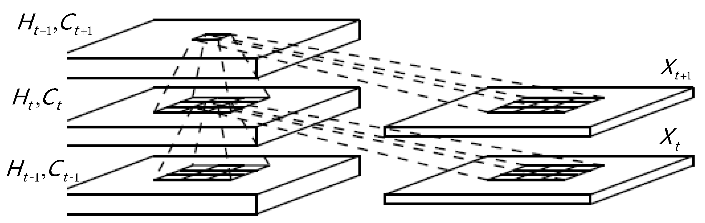
Convolutional neural networks (CNNs) have powerful capabilities of extracting spatial features and can automatically extract universal features through back-propagation algorithms driven by dataset [30,31], however they cannot be used to process sequence signals directly for the reason that the input is independent with each other, and the information flows strictly in one direction from layer to layer.To solve this problem, we introduce convolutional long short-term memory (ConvLSTM) [32] to the network, the inner structure of ConvLSTM is shown in Figure 1. As a special kind of RNN, long short-term memory network (LSTM) has internal hidden memory which allows the model to store information about its past computations and capable of learning long-term dependency [33]. Different than standard LSTM, all of the features variables of ConvLSTM including the input $X_t$, cell state $C_t$, the output of the forget gate $F_t$, input gate $i_t$, and output gate $O_t$ are three-dimensional tensors, the latter two of which are spatial dimensions width and height. The key equations of ConvLSTM are defined as:

$$\begin{array}{cc}\hfill F_t& =\sigma (W_f[H_{t-1},X_t]+b_f),\hfill \\ \hfill i_t& =\sigma (W_i[H_{t-1},X_t]+b_i),\hfill \\ \hfill {\tilde{C}}_t& =tanh(W_C[H_{t-1},X_t]+b_c),\hfill \\ \hfill C_t& =F_t*C_{t-1}+i_t*{\tilde{C}}_t,\hfill \\ \hfill O_t& =\sigma (W_o[H_{t-1},F_t]+b_o),\hfill \\ \hfill H_t& =O_t*tanh\left(C_t\right),\hfill \end{array}$$

(6)

where “*" and “$\sigma$" denote the Hadamard product and the logistic sigmoid function, respectively. $F_t$ controls the abandoned state information of the last layer and $i_t$ is in charge of current state update, i.e., ${\tilde{C}}_t$. $W_f$, $W_i$, $W_c$, and $W_o$ represent weights of each neural unit with $b_f$, $b_i$, $b_c$, and $b_o$ denoting the corresponding offsets.

3. Proposed Method

An end-to-end network MSR-net for SAR image despeckling is proposed in this paper. Rather than using additional division operation [25,26] or subtraction operation [9,27], our network can automatically perform despeckling and generate a clean image. In this section, we first introduce the multi-scale recurrent architecture and then describe specific details through a single-scale model.

3.1. Architecture

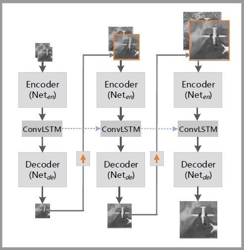
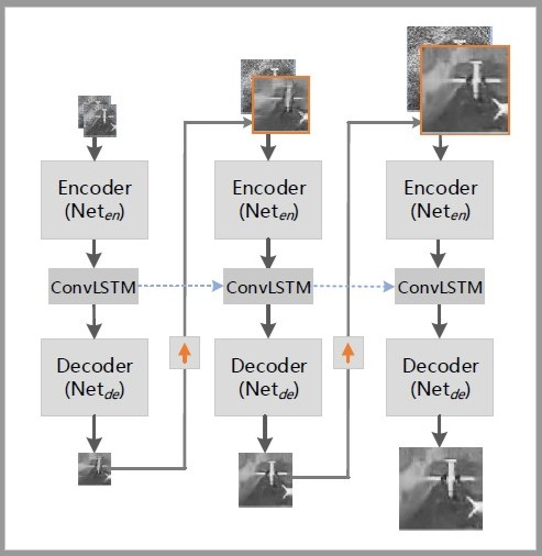
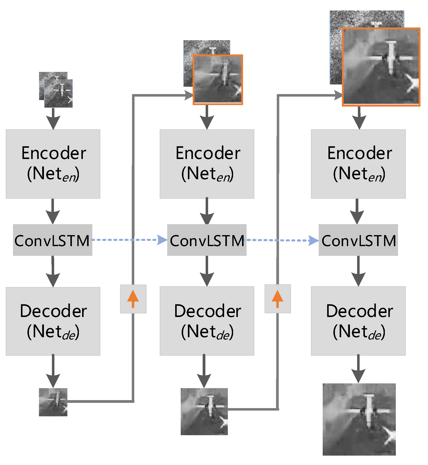
MSR-net is built based on cascaded subnetworks, and each subnetwork contains three parts: encoder, decoder, and ConvLSTM unit, as illustrated in Figure 2. Different levels of subnetworks correspond to different scales of inputs and outputs. The next scale speckled image and the output of current subnetwork are combined as the input of next-level subnetwork. In addition, an LSTM unit with single input and two-output is embedded between encoder and decoder. Specifically, one output is connected to the decoder, and the other output which represents the hidden state is connected to LSTM unit of the next subnetwork.

Different from the general cascaded network like [34], which uses three stages of independent subnetworks, all the state features flow across scales and share the same training parameters in MSR-net. Owing to the multi-scale recurrent and parameter share strategy, the number of parameters that need to be trained in MSR-net is only 1/3 of [34].

For the subnetwork, the output ${\mathbf{F}}^i$ of encoder ${\mathbf{Net}}_{en}$, which takes the speckled image and despeckled result up-sampled from the previous scale as input, can be defined as:

$${\mathbf{F}}^i={\mathbf{Net}}_{en}\left({\mathbf{I}}_{in}^i,up\left({\mathbf{I}}_o^{i+1}\right);{\Theta }_{en}\right),$$

(7)

where ${\mathbf{I}}_{in}^i$ is the input image with speckle noise, ${\Theta }_{en}$ is the weights parameters of ${\mathbf{Net}}_{en}$. $i=0,1,2,...$ is the scale index. The larger i is, the lower the resolution is. $i=0$ represents the original resolution and $i=1$ indicates down sampling once. ${\mathbf{I}}_o^{i+1}$ is the output of the previous coarse scale. $up(·)$ is the operator that adapts features or images from the (i + 1)-th to the i-th scale, which is implemented by bilinear interpolation.

To exploit the information contained in feature maps of different scales, a convolutional LSTM module is embedded between the encoder and the decoder. The ConvLSTM can be defined as:

$${\mathbf{h}}^i,{\mathbf{g}}^i=\mathbf{ConvLSTM}\left(up\left({\mathbf{h}}^{i+1}\right),{\mathbf{F}}^i;{\Theta }_{LSTM}\right),$$

(8)

where ${\Theta }_{LSTM}$ is the set of parameters in ConvLSTM, ${\mathbf{h}}^i$ is the hidden state which is passed to the next scale, ${\mathbf{h}}^{i+1}$ is the hidden state from the previous scales, and ${\mathbf{g}}^i$ is the output of the current state (scale). Finally, we use ${\Theta }_{de}$ to denote the parameters of the decoder, and the output can be defined as:

$${\mathbf{I}}_o^i={\mathbf{Net}}_{de}\left({\mathbf{g}}^i;{\Theta }_{de}\right).$$

(9)

3.2. Single Scale Network

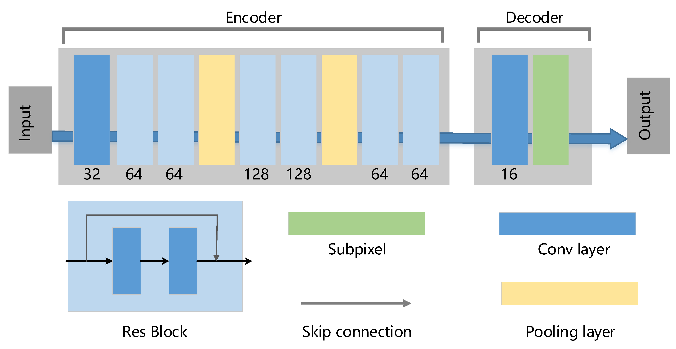
Details of the MSR-net are introduced by the single-scale model in this section. As shown in Figure 3, the single-scale model consists of two parts: encoder and decoder. The encoder includes three building blocks: convolutional layer, pooling layer, and Res block.

The convolution unit performs convolution operation and non-linear activation. Increasing the number of convolutional layers can enhance the feature extraction ability [35,36]. Multiple Res blocks are added after the convolutional layer while designing the network. Unlike the convolution unit, skip connection proposed by He et al. [37] is built into this block, which can effectively avoid gradient explosion or gradient disappearance, as well as increasing the training speed.

The size of the input and output of the convolutional layers keeps the same as the despeckling networks designed in [6,25,27], which increases the amount of computation to a certain extent. We reduce the amount of calculation by decreasing the dimension of the feature maps, i.e., adopting the pooling layer. We choose max pooling operation with the $2\times 2$ pooling kernel in this layer. It should be noted that the pooling layer can also be replaced by strided convolutions [38].

The decoder consists of the convolutional layer and the sub-pixel units. The width and height of the input feature map to the decoder are only $1/4$ of the original image after down-sampling twice through the pooling layer. Therefore, the up-sampling operation is required to make the output image of the network the same as the input size. However, an up-sampling operation such as transposed convolution used in [39,40] needs a high amount of computation and causes unwanted checkerboard artifacts [41,42]. A typical checkerboard pattern of artifacts is shown in Figure 4. To reduce the network runtime and avoid the checkerboard pattern of artifacts, the sub-pixel convolution described in Section 3.3 is used to implement the up-sampling operation.

3.3. Sub-Pixel Convolution

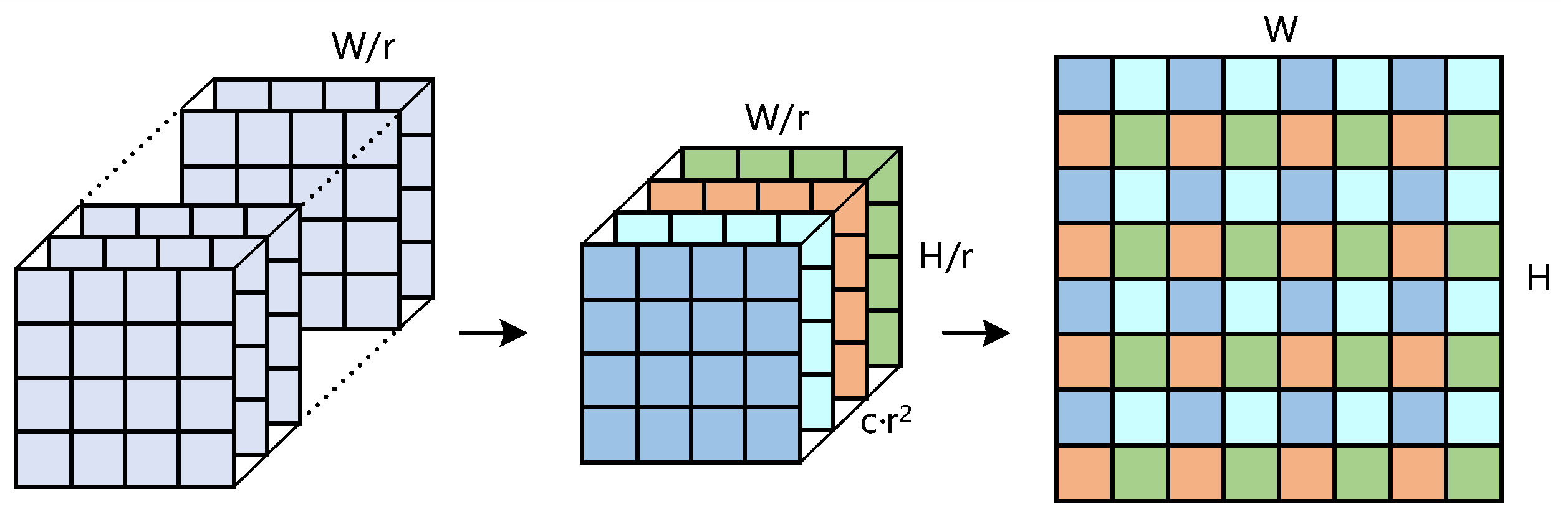
Sub-pixel convolution, also called as pixel shuffle, is an upscaling method first proposed in [43] for image super-resolution tasks. Different from the commonly used up-sampling methods in deep learning such as transposed convolution and fractionally strided convolution, sub-pixel convolution adopts channel to space method which achieves spatial scale-up amplification by rearranging pixels in multiple channels of the feature map, as illustrated in Figure 5.

For a sub-pixel unit with r times up-sampling, its output image is defined as ${\mathbf{I}}^{up}$, and we have ${\mathbf{I}}^{up}\in {\mathbb{R}}^{W\times H\times c}$, in which W, H, and c denote the width, height and channels of ${\mathbf{I}}^{up}$. The sub-pixel convolution operation is defined as:

$${\mathbf{I}}^{up}(x,y,c)=\mathbf{F}\left(\lfloor x/r\rfloor ,|y/r\rfloor ,c·r·mod(y,r)+c·mod(x,r)+c\right)$$

(10)

where ${\mathbf{I}}^{up}(x,y,c)$ is the value of the pixel at the position (x,y) for the c$th$ channel. $\mathbf{F}$ is the input of sub-pixel and $\mathbf{F}\in {\mathbb{R}}^{W/r\times H/r\times c{r}^2}$. $\lfloor ·\rfloor$ represents floor function that takes as input a real number and gives as output the greatest integer less than or equal to it [43]. After sub-pixel convolution operation, the elements of $\mathbf{F}$ are rearranged to the output ${\mathbf{I}}^{up}$ by increasing the horizontal and vertical count, and decreasing channel count. For example, when a $64\times 64\times 4$ feature map is passed through the sub-pixel unit, an output with shape $128\times 128\times 1$ will be obtained.

3.4. Proposed Evaluation Criterion

In this paper, the peak signal to noise ratio (PSNR) [44], structural similarity (SSIM) [45], equivalent number of looks (ENL) [46], and two new proposed evaluation criterions edge feature keep ratio (EFKR) and feature point keep ratio (FPKR) are used to evaluate the performance of despeckling methods.

PSNR is the ratio between the maximum possible power of a signal and the power of corrupting noise that affects the fidelity of its representation, which has been widely used in quality assessment of reconstructed images. SSIM is a metric of image similarity. ENL can describe the smoothness of regions, and no reference image is needed for its calculation, so it can be used to evaluate the performance of despeckling methods for real SAR images.

Edge Feature Keep Ratio and Feature Point Keep Ratio

PSNR and SSIM can effectively evaluate the overall performance of despeckling methods. Specifically, PSNR measures noise level or image distortion, SSIM measures the similarity between two images, and ENL measures the degree of region smoothing. They are not, however, capable of evaluating the edge and typical features retention ability in despeckling tasks directly. In this section, we propose two evaluation criteria that can compensate for the above deficiencies, i.e., edge feature keep ratio (EFKR) and feature point keep ratio (FPKR).

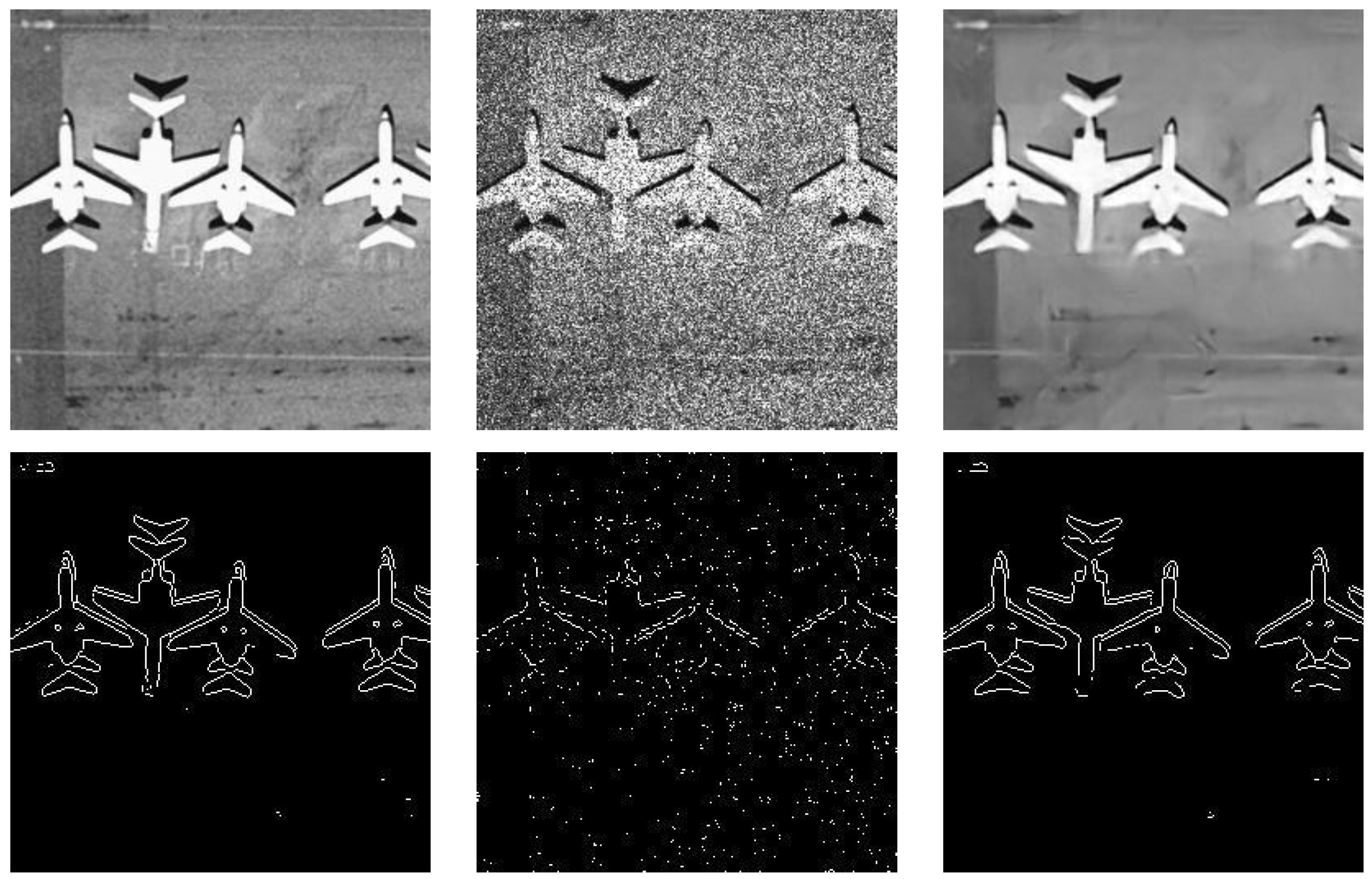
(a) EFKR: from the edge detection results shown in Figure 6, we have the following observations. (1) The edge outline of the speckled image is blurred, and there are discrete points in the image; (2) the edge outline is clear after despeckling and there is no discrete point, which is in agreement with the edge detection results of a clean image. Enlightened by this phenomenon, we design a quantitative evaluation criterion EFKR with the ability of edge retention based on counting the number of pixels of edges. The computation steps are as follows:

• Edge detection processing for clean and test image using edge detection algorithms such as Sobel [47], Canny [48], Prewitt [49], and Roberts [50] methods. After this, two images only with only edge lines are obtained. The values of pixels in the edge position are set to 1, the values of the other position are set to 0.
• Bit-wise and operation on two images from step 1, values at the position where the edges coincide are set to 1, values at other locations are set to 0.
• Count the number of value 1 in the edge detected the result of a clean image and the number of 1 in step 2, and calculate the ratio of the two numbers.

The ratio of these two factors is the edge feature retention ratio, which is defined as:

$$EFKR=\frac{sum\left(\mathbf{edge}\right(X)\&\mathbf{edge}(Y\left)\right)}{sum\left(\mathbf{edge}\right(Y\left)\right)},$$

(11)

where & and $sum$ denotes the bit-wise conjunction operation and sum operation, and $\mathbf{edge}$ represents edge detection.

(b) FPKR: for real SAR images, ENL is only able to evaluate the smooth level but not the retention ability of typical features such as edges, corners in the image. SIFT [51] can find feature points from different scales and obtain the ultimate descriptor of features. Also, the key points found by SIFT are usually corner points, edge points, bright spots in dark areas, and dark points in bright areas. These points are robust to light, affine transformations, and other transformation. The registration method based on SIFT first uses SIFT to obtain the feature points of the image to be registered, the reference image and their descriptor then matches the feature points according to descriptor and obtains one-to-one corresponding feature point pairs. Finally, the transformation parameters are calculated, and the image registration is carried out.

For SAR images, the registration of feature points and descriptors at the lights spots of speckles are redundant, which also reduce the efficiency and accuracy of subsequent searching of matching points. Based on this phenomenon, we design an evaluation criterion FPKR targeting at key feature points. We first execute an affine transformation to the evaluation image, then use the SIFT algorithm to find the feature points in the two images before and after the transformation, and finally match the feature points. The better the despeckling performs, the more typical features are preserved. The more prominent the feature descriptor obtained by SIFT, the greater the difference of descriptor between different features, so more effective feature point pairs can be searched efficiently. FPKR is defined as:

$$FPKR=\frac{N_{match}(X,X_t)}{min(N\left(X\right),N\left(X_t\right))}$$

(12)

where $N\left(X\right),N\left(X_t\right)$ are the number of key points before and after SIFT, and $N_{match}(X,X_t)$ denotes the number of points for calculating transformation parameters.

4. Experiments and Results

4.1. Dataset

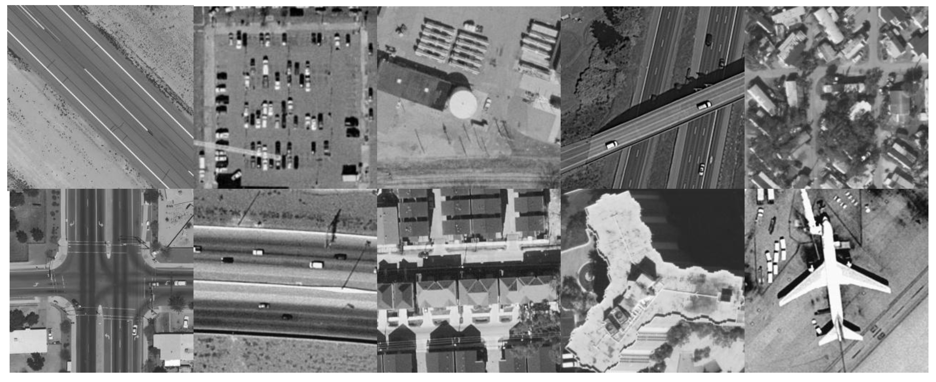
Because it is hard to collect real SAR images without speckle noise, we train networks by using synthetic noise/clean image pairs. Public dataset UC Merced Land Use Dataset (http://weegee.vision.ucmerced.edu/datasets/landuse.html) is chosen as the original clean image for training. The dataset contains 21 scene classes with 100 optical remote sensing images per class. Each image has a size of $256\times 256$ pixels and the pixel resolution is 1 foot [52]. According to [27], we randomly select 400 images from the dataset as the training set and use the remaining images for testing. Some training samples are shown in Figure 7. Finally, after grayscale preprocessing, the speckled images are generated using Equation (1) same as the [25,53]. The noise levels (L = 2, 4, 8, 12) correspond to the number of looks in SAR, and the code of adding speckle noise is available on GitHub (https://github.com/rcouturier/ImageDenoisingwithDeepEncoderDecoder/tree/master/data{_}denoise).

4.2. Experimental Settings

All the networks are trained with stochastic gradient descent (SGD) with a mini-batch size of 32. All weights are initialized by a modified scheme of Xavier initialization [54] proposed by He et al. Meanwhile, we use the Adam optimizer [55] with tuned hyper-parameters to accelerate training. The hyper-parameters are kept the same across all layers and all networks. Experiments are implemented on TensorFlow platform with Intel i7-8700 CPU and an NVIDIA GTX-1080(8G) GPU.

The details of the model are specified here. The number of kernels in each unit is shown in Figure 3. The kernel sizes for the first and last convolutional layers are $5\times 5$, while all others are $3\times 3$. Rectified Linear Units (ReLU) are used as the activation function for all layers except for the last convolutional layer before sub-pixel unit. The ${\mathcal{L}}_1$ loss is chosen to train the network, which is defined as:

$${\mathcal{L}}_1(\Theta )=\frac{1}{N}\sum _{y=1}^W\sum _{x=1}^H|\phi \left(\mathbf{X}(x,y);\Theta \right)-\mathbf{C}(x,y)|,$$

(13)

where $\Theta$ is the filter parameters that need to be updated during training, $\mathbf{C}$, $\mathbf{X}$ and $\phi \left(·\right)$ denote the objective image without noise, the input image with speckle noise, and the output after despeckling, respectively.

4.3. Experimental Results

The test results of our proposed network will be presented in this section. To verify the proposed method, we compare the performance of our MSR-net with other three despeckling methods, SAR-BM3D [22], ID-CNN [25], and Residual Encoder-Decoder network (RED-NET) [53]. The first one is a traditional nonlocal algorithm based on wavelet shrinkage, and the latter two methods are based on deep convolutional neural networks.

4.3.1. Results on Synthetic Images

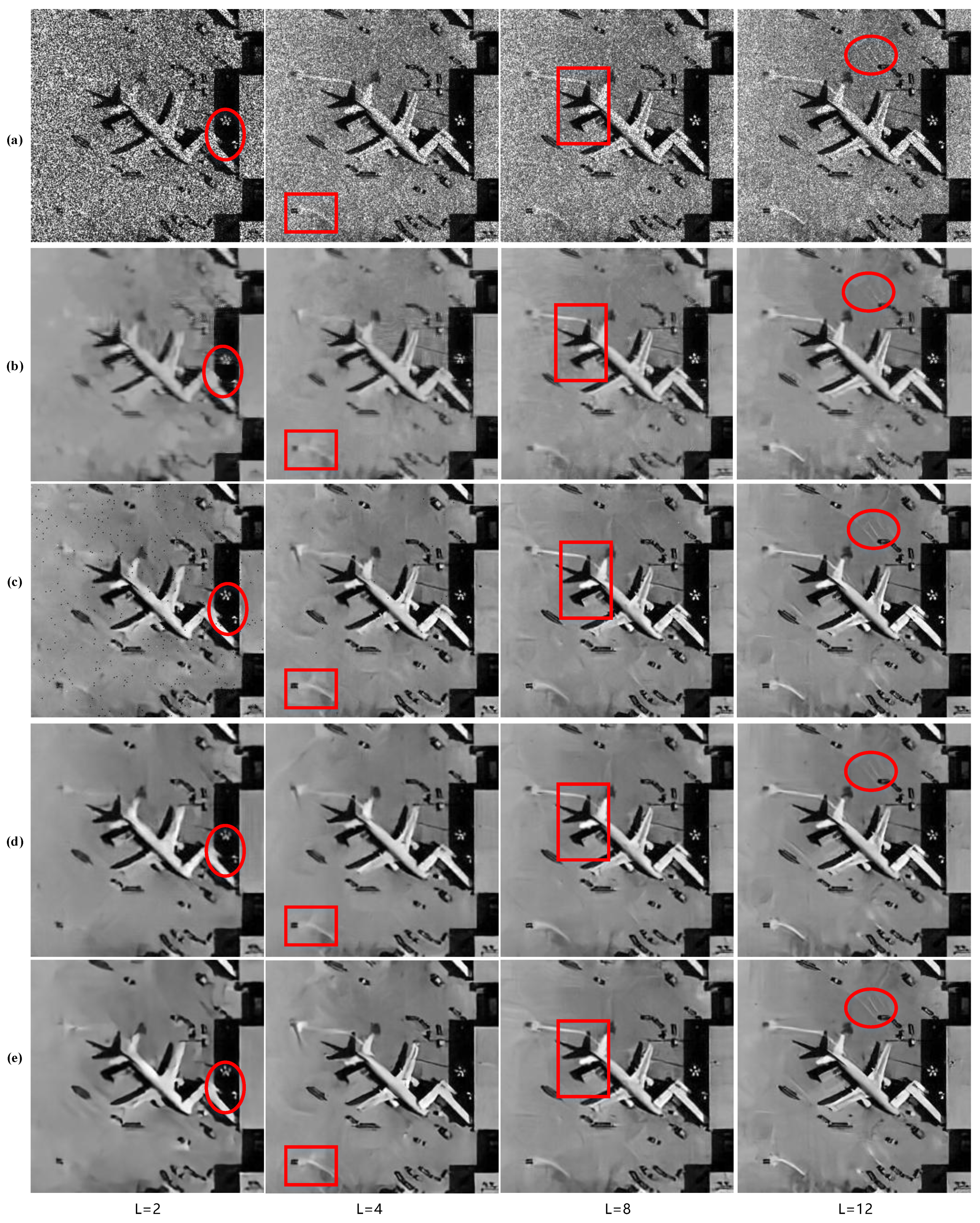
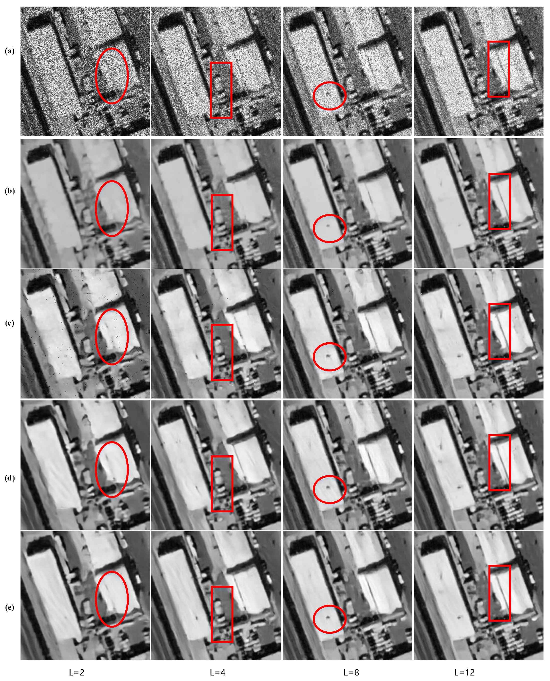
Building, freeway, and airplane, three classes of synthetic images, are chosen as the test set to evaluate the noise reduction ability of each method. Part of the processing results of different algorithms under different levels of noise are shown in Figure 8 and Figure 9.

From the figures, we can observe that the CNN-based methods, including our MSR-net, can preserve more details like texture features in images than SAR-BM3D after despeckling. When the noise is strong, the SAR-BM3D algorithm will cause blurring at the edge of the objects.

ID-CNN has a good performance on image despeckling, however, after filtering by the network, pepper and salt noise appear in the image, which needs to be processed subsequently by using nonlinear filters such as median filtering and pseudo-median filtering. As the noise intensity increases, the salt and pepper noise increase gradually.

MSR-net has excellent retention performance of spatial geometry features like texture features, lines, and feature points. Compared with the other three algorithms, MSR-net has a higher smoothness of smooth areas as well as a smaller loss of sharpness of edges and details, especially for strong speckle noise. Also, more detail information in image will loose when the speckle noise is strong and more local detail can be preserved in output images when the speckle noise is weak.

When the level of noise added to the test set is small, all the CNN-based approaches can get state-of-art results. Therefore, it is difficult to judge the merits of these algorithms by using visual assessments. Experimental results of evaluation indexes such as PSNR and SSIM are necessary for these circumstances. The PSNR, SSIM, and EFKR evaluation indexes of the above methods are listed in

Table 1. The peak signal to noise ratio (PSNR), structural similarity (SSIM), and edge feature keep ratio (EFKR) of test set with noise level L = 2.

Classes	Index	SAR-BM3D	ID-CNN	RED-Net	SS-Net	MSR-Net
	PSNR	20.343 ± 0.043	21.639 ± 0.073	22.321 ± 0.065	22.467 ± 0.039	22.768 ± 0.052
building	SSIM	0.579± 0.005	0.599 ± 0.002	0.672 ± 0.005	0.663 ± 0.002	0.684 ± 0.004
	EFKR	0.3872± 0.061	0.3888 ± 0.058	0.5131 ± 0.053	0.4950± 0.040	0.5322 ± 0.049
	PSNR	22.478 ± 0.081	23.17± 0.046	25.157± 0.033	25.255 ± 0.057	25.526± 0.064
freeway	SSIM	0.581 ± 0.002	0.536 ± 0.003	0.662 ± 0.003	0.663 ± 0.048	0.680 ± 0.002
	EFKR	0.3046± 0.052	0.3376 ± 0.061	0.5071 ± 0.061	0.4929 ± 0.064	0.5065 ± 0.057
	PSNR	21.351± 0.045	24.006 ± 0.058	23.97± 0.062	24.166 ± 0.046	24.433± 0.049
airplane	SSIM	0.602 ± 0.004	0.641 ± 0.003	0.638 ± 0.001	0.636 ± 0.002	0.649 ± 0.005
	EFKR	0.3048± 0.069	0.2965 ± 0.073	0.4929 ± 0.063	0.4800 ± 0.058	0.5123 ± 0.065

The bold number represents the optimal value in each row, while the underlined number denotes the suboptimal value in each row.

,

Table 2. The PSNR, SSIM, and EFKR of test set with noise level L = 4.

Classes	Index	SAR-BM3D	ID-CNN	RED-Net	SS-Net	MSR-Net
	PSNR	21.789 ± 0.046	24.319 ± 0.101	24.366 ± 0.059	24.279 ± 0.032	24.370± 0.038
building	SSIM	0.694 ± 0.003	0.721 ± 0.005	0.737 ± 0.006	0.722 ± 0.001	0.735 ± 0.005
	EFKR	0.5029± 0.059	0.5459± 0.057	0.5646± 0.050	0.5742± 0.0423	0.6021± 0.051
	PSNR	24.351 ± 0.059	26.008 ± 0.051	26.821 ± 0.063	26.734 ± 0.030	26.893 ± 0.049
freeway	SSIM	0.645 ± 0.003	0.670 ± 0.002	0.718 ± 0.005	0.711 ± 0.003	0.722 ± 0.003
	EFKR	0.4897± 0.061	0.5019± 0.060	0.5469± 0.057	0.5511± 0.065	0.5608± 0.051
	PSNR	23.261 ± 0.041	25.747 ± 0.067	25.849 ± 0.050	25.905 ± 0.046	26.046 ± 0.064
airplane	SSIM	0.657 ± 0.003	0.677 ± 0.005	0.691 ± 0.004	0.686 ± 0.002	0.693 ± 0.005
	EFKR	0.4976± 0.061	0.5149 ± 0.058	0.5484 ± 0.056	0.5728 ± 0.039	0.5871 ± 0.055

The bold number represents the optimal value in each row, while the underlined number denotes the suboptimal value in each row.

,

Table 3. The PSNR, SSIM, and EFKR of test set with the noise level L = 8.

Classes	Index	SAR-BM3D	ID-CNN	RED-Net	SS-Net	MSR-Net
	PSNR	23.851 ± 0.071	26.004 ± 0.055	25.685 ± 0.043	25.989 ± 0.064	26.026 ± 0.048
building	SSIM	0.752 ± 0.003	0.780 ± 0.002	0.769 ± 0.05	0.774 ± 0.004	0.782 ± 0.004
	EFKR	0.5992± 0.065	0.6191± 0.055	0.6305± 0.050	0.6261± 0.0525	0.6476± 0.060
	PSNR	26.374 ± 0.081	27.738 ± 0.049	27.785 ± 0.068	28.027 ± 0.053	28.111 ± 0.057
freeway	SSIM	0.714 ± 0.003	0.740 ± 0.006	0.751 ± 0.006	0.753 ± 0.004	0.757 ± 0.003
	EFKR	0.5432± 0.041	0.5809± 0.053	0.5990± 0.052	0.5890 ± 0.057	0.5954± 0.048
	PSNR	25.31 ± 0.064	27.438 ± 0.051	27.161 ± 0.044	27.404 ± 0.061	27.443 ± 0.042
airplane	SSIM	0.71 ± 0.005	0.731 ± 0.004	0.720 ± 0.004	0.728 ± 0.005	0.732 ± 0.002
	EFKR	0.5872± 0.057	0.6039 ± 0.047	0.6113 ± 0.053	0.6187 ± 0.038	0.6293 ± 0.051

The bold number represents the optimal value in each row, while the underlined number denotes the suboptimal value in each row.

and

Table 4. The PSNR, SSIM, and EFKR of test set with the noise level L = 12.

Classes	Index	SAR-BM3D	ID-CNN	RED-Net	SS-Net	MSR-Net
	PSNR	24.979 ± 0.060	26.891 ± 0.043	26.879 ± 0.056	26.929 ± 0.071	26.942 ± 0.052
building	SSIM	0.781 ± 0.004	0.805 ± 0.0002	0.805 ± 0.004	0.802 ± 0.005	0.806 ± 0.003
	EFKR	0.6184± 0.051	0.6441± 0.049	0.6528± 0.047	0.6596± 0.054	0.6664± 0.058
	PSNR	27.444 ± 0.042	28.643 ± 0.059	28.905 ± 0.047	28.787 ± 0.066	28.893 ± 0.050
freeway	SSIM	0.747 ± 0.003	0.768 ± 0.006	0.782 ± 0.007	0.776 ± 0.004	0.778 ± 0.005
	EFKR	0.5975± 0.056	0.6130± 0.053	0.6218± 0.056	0.6247± 0.067	0.6197± 0.051
	PSNR	26.463 ± 0.053	28.362 ± 0.64	28.352 ± 0.078	28.349 ± 0.059	28.407 ± 0.065
airplane	SSIM	0.737 ± 0.005	0.756 ± 0.003	0.758 ± 0.003	0.754 ± 0.005	0.756 ± 0.006
	EFKR	0.6008± 0.059	0.6275 ± 0.057	0.6432 ± 0.052	0.6465 ± 0.052	0.6433 ± 0.053

The bold number represents the optimal value in each row, while the underlined number denotes the suboptimal value in each row.

, respectively. The bold number represents the optimal value in each row, while the underlined number denotes the suboptimal value. We also test MSR-net with only one scale and call it a single scale network (SS-net) during the experiment.

Consistent with the results shown in Figure 8 and Figure 9, our method has much better speckle-reduction ability than non-learned approach SAR-BM3D at different noise levels. In addition, the advantage of MSR-net will increase as the noise level increases. Taking airplane images for instance, the PSNR/SSIM/EFKR of our proposed MSR-net outperform SAR-BM3D by about 3.082 dB/0.047/0.2075, 2.785 dB/0.036/0.0895, 2.133 dB/0.022/0.0421, 1.944 dB/0.019/0.0425 for L = 2, 4, 8, 12.

Compared with CNN-based methods, MSR-net still has an advantage when the noise is strong. When L = 2, the PSNR/SSIM/EFKR of MSR-net outperform ID-CNN, RED-Net by about 1.129 dB/0.014/0.1434, 2.356 dB/0.144/0.1689, 0.427 dB/0.008/0.2152 and 0.447 dB/0.012/0.0191, 0.369 dB/0.018/-0.006, 0.643 dB/0.011/0.0194 for building, freeway, and airplane, respectively. When L = 4, the PSNR/SSIM/EFKR of MSR-net outperform ID-CNN, RED-Net by about 0.051 dB/0.134/0.0562, 0.885 dB/0.052/0.0589, 0.299 dB/0.016/0.0722 and 0.004 dB/-0.002/0.0375, 0.072 dB/0.004/0.0139, 0.197 dB/0.002/0.0143 for building, freeway and airplane, respectively.

In addition, we can see that our network does not always achieve the best test results. We consider this may have a certain relationship with the feature distribution of the images. Although MSR-net can only get sub-optimal test results for a certain class of images, the difference to the best result is small. For other classes of images, the advantages of MSR-net are more considerable. For example, we can observe from Table 1 that the EFKR of RED-Net only outperforms MSR-net by about 0.006 for freeway images, while MSR-net can outperform RED-Net by about 0.0191 and 0.0194 for building and airplane images. When the noise level L = 12, our network only gets four best test values, which suggests the advantage of the multi-scale network becomes smaller while the noise is weaker, as shown in Table 4.

MSR-net with a single scale (SS-net) also has very good speckle-reduction ability. When the noise intensity is weak, the performance is even better than multi-scale. For example, when L = 12, PSNR/SSIM/EFKR of the freeway are 28.787 dB/0.776/0.6247 and 28.893 dB/0.778/0.6197 for SS-net and MSR-net, respectively. Ultimately, we can find by comparison that the edge detection effect of the image has been significantly improved after despeckling.

4.3.2. Results on Real Sar Images

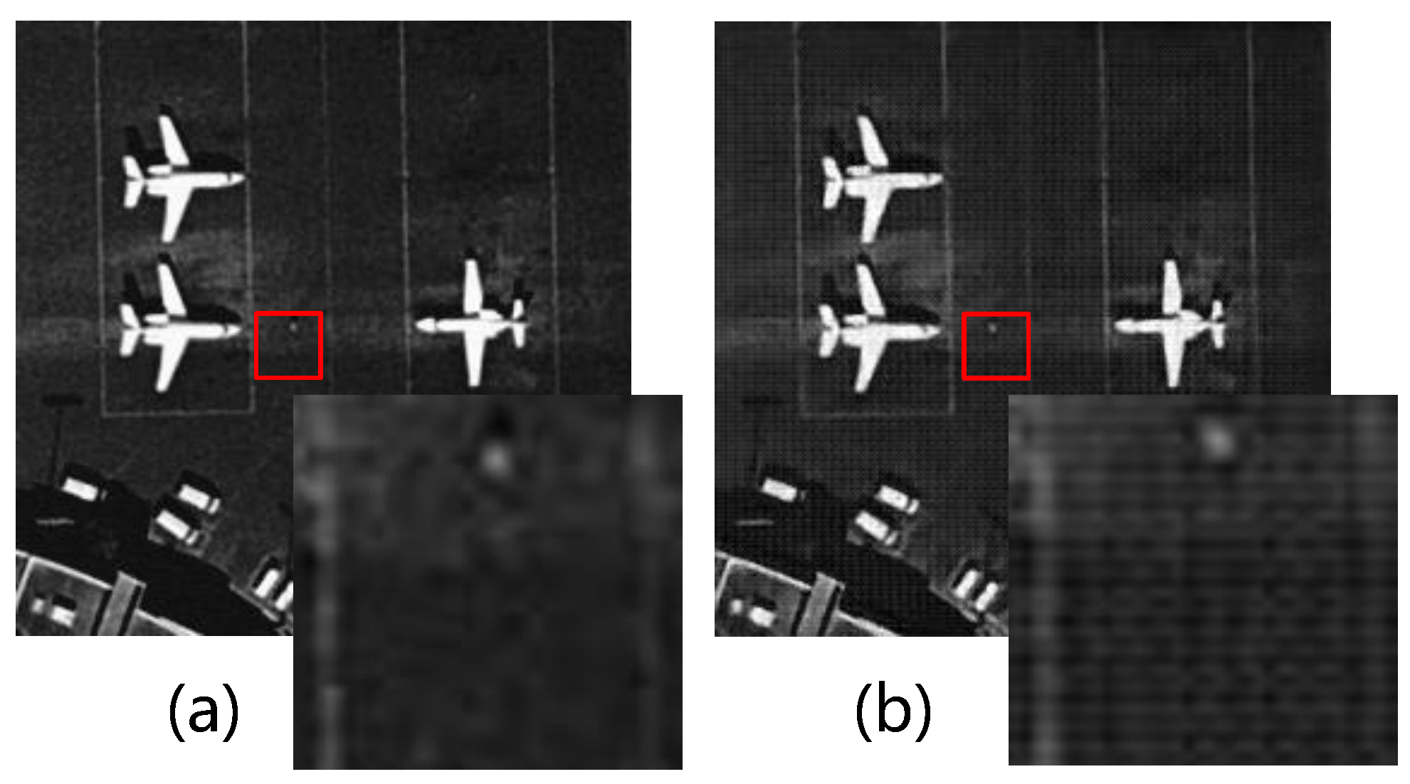
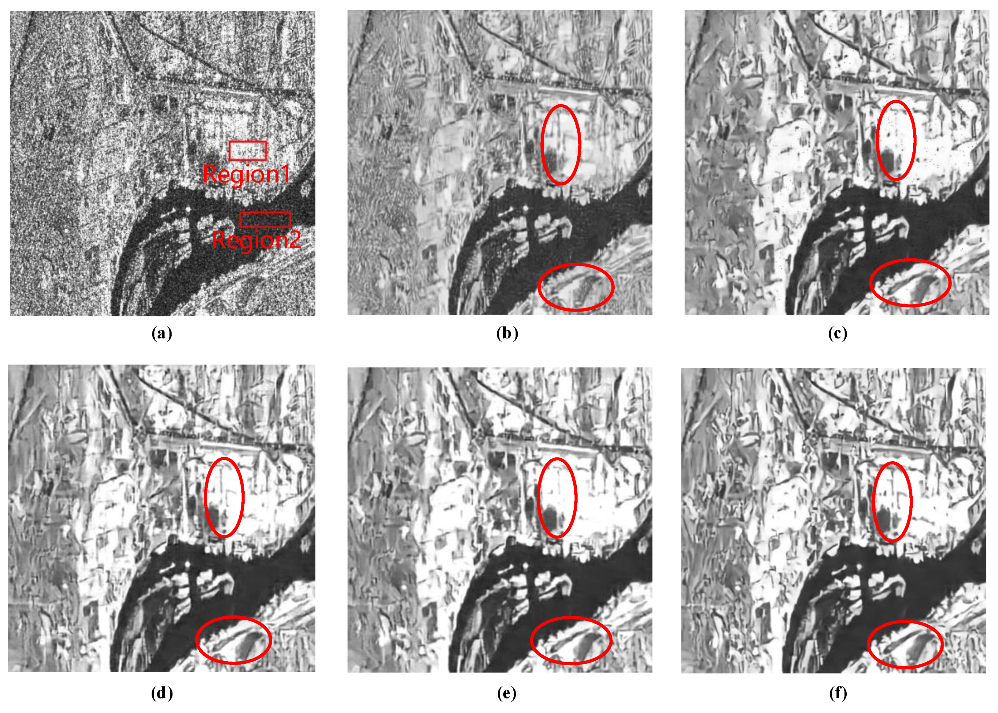
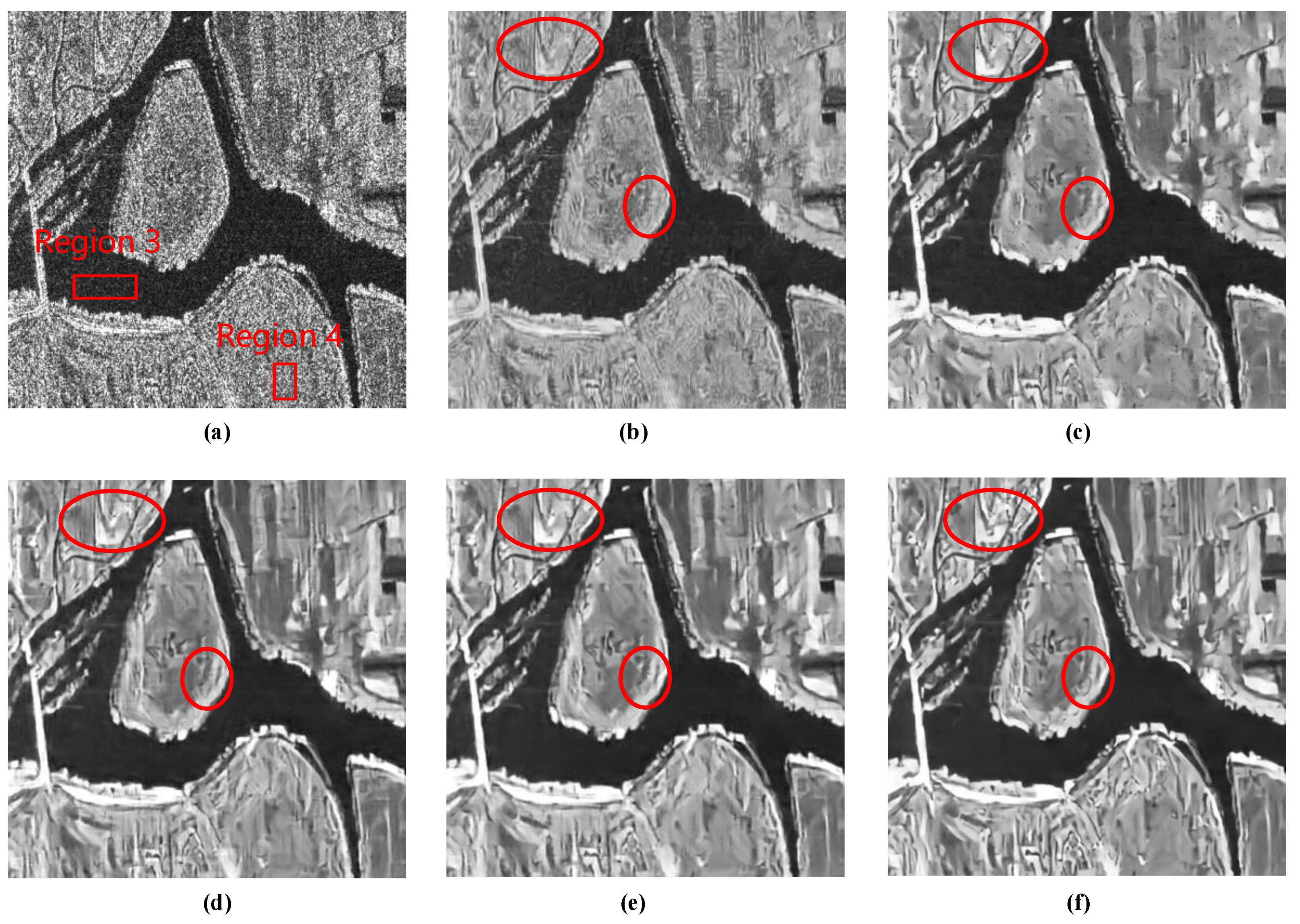
To further verify the speckle-reduction ability of our network for real SAR images, two SAR sceneries are selected, as shown in Figure 10a and Figure 11a, and these two images are imaging results of spaceborne SAR RADARSAT-2.

It can be seen by comparing the subgraphs in Figure 10 and Figure 11 that MSR-net generates the visually best output among all the results and retains the edge sharpness as well as the detail information about the structure in the image while removing the speckle noise. After filtering by SAR-BM3D, the loss of edge sharpness of the original SAR image is obvious and most of the lines and texture feature are blurred. ID-CNN and RED-Net can generate smooth results in homogeneous regions while maintaining textural features in the image. However, from the red boxes, we can observe that they are capable of retaining some texture features but not better than MSR-net. Although SS-net performs well in despeckling for real SAR images, it is still worse than multi-scale MSR-net.

The ENL results are shown in

Table 5. The equivalent number of looks (ENL) of real SAR regions

Data	Original	SAR-BM3D	ID-CNN	RED-Net	SS-Net	MSR-Net
region1	3	51	104	317	394	540
region2	51	195	173	413	2906	644
region3	3	80	101	333	339	622
region4	4	99	95	235	369	560

The bold number represents the optimal value in each row.

. We can observe from the table that MSR-net has an outstanding performance for real SAR image despeckling. For these four evaluation regions, the three highest scores and one second highest score of the ENL are obtained by our MSR-net.

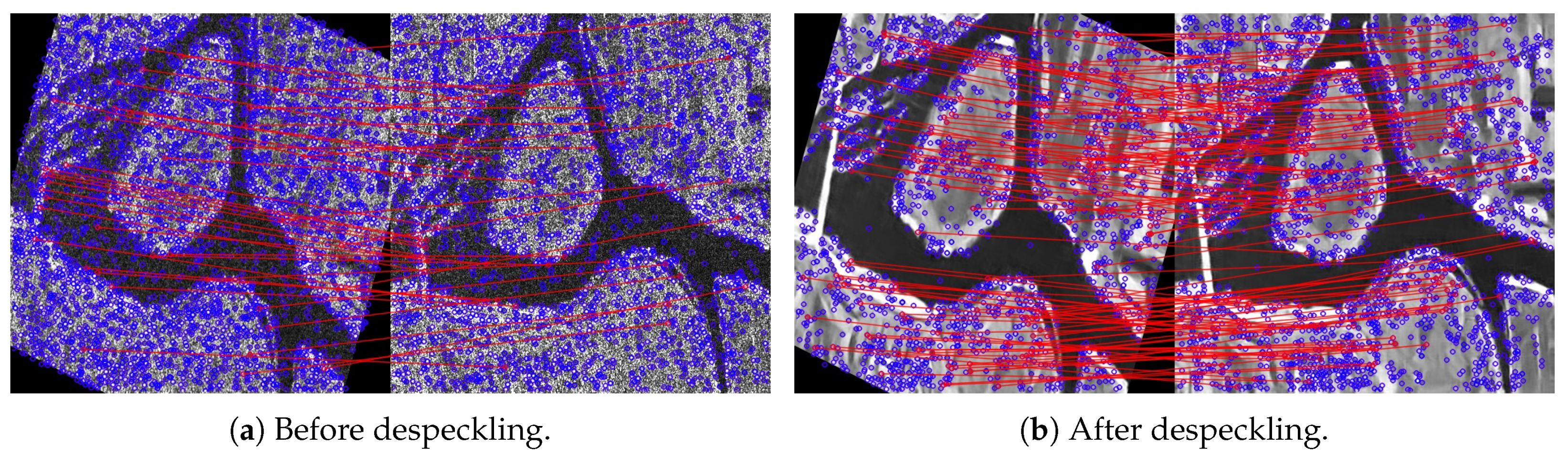
To achieve FPKR results for real SAR data with different methods, we first apply the same affine transformation to each image, as shown in Figure 12. SIFT is then applied to search for the feature points and calculate their descriptors. Matching key points are ultimately conducted by minimizing the Euclidean distance between their SIFT descriptors. Generally, the ratio between distances is used [56] to obtain high matching accuracy. In the experiments, we select three ratios and the FPKR results are shown in

Table 6. Feature point keep ratio (FPKR) results before and after despeckling for real SAR image.

	fp1	fp2	FPKR (r = 0.25)	FPKR (r = 0.30)	FPKR (r = 0.35)
original	5637	4531	0.0004 ( 2 )	0.0077 ( 35 )	0.0362 (164)
SAR-BM3D	4554	5947	0.0046 (21)	0.0212 (110)	0.0894 (407)
ID-CNN	3233	3981	0.0049 (16)	0.0294 ( 95 )	0.1148 (371)
RED-Net	3636	4644	0.0055 (20)	0.0292 (106)	0.0976 (355)
SS-Net	3429	4357	0.0052 (18)	0.0286 ( 98 )	0.1155 (396)
MSR-net	3080	4216	0.0071 (22)	0.0425 (106)	0.0981 (302)

The value inside brackets is the number of feature points. The bold number represents the optimal value in each column.

and

Table 7. FPKR results before and after despeckling for real SAR image.

	fp1	fp2	FPKR (r = 0.25)	FPKR (r = 0.30)	FPKR (r = 0.35)
original	4511	3476	0.0012 ( 4 )	0.0118 ( 41 )	0.0437 (152)
SAR-BM3D	3878	5289	0.0044 (17)	0.0273 (106)	0.0952 (369)
ID-CNN	2021	2533	0.0124 (25)	0.0574 (116)	0.1366 (267)
RED-Net	2137	2797	0.0140 (30)	0.0543 (116)	0.1526 (326)
MSR-net	2021	2533	0.0166 (33)	0.0674(134)	0.1579 (314)

The value inside brackets is the number of feature points. The bold number represents the optimal value in each column.

. By comparing EFKR of each image, MSR-net performs better than SAR-BM3D. Also, MSR-net shows advantages over other neural network-based algorithms. Specifically, MSR-net achieves the best testing results in five out of six sets of experiments. It also indicates that pre-processing to SAR images by MSR-net can effectively enhance the usefulness of SIFT algorithm to SAR images and improve its performance and efficiency.

4.3.3. Runtime Comparisons

To evaluate the algorithm efficiency, we make statistics of the runtime of each algorithm in CPU implementation. The runtime of different methods on images with different sizes is listed in

Table 8. Runtime (s) of different methods of images with sizes of $256\times 256$ and $512\times 512$.

Size	SAR-BM3D	ID-CNN	RED-Net	SS-Net	MSR-Net
$256\times 256$	12.79	0.448	2.241	0.339	0.586
$512\times 512$	52.813	1.562	8.943	1.342	2.375

. We can see that the proposed denoiser is very competitive although its structure is relatively complex. Such a good compromise between speed and performance over MSR-net is properly attributed to the following two reasons. First, two pooling layers that can achieve spatial dimensionality reduction are embedded in the MSR-net. Each pooling layer with the $2\times 2$ pooling kernel can reduce the amount of data that needs to be processed by the subsequent convolution operation to 25% of before. Second, in contrast to the transposed convolution which increases the resolution of feature maps by padding and complex convolution operation, sub-pixel unit, which up-samples feature maps by a periodic shuffling of pixel values, is adopted to build our network.

5. Discussion

5.1. Choice of Scales

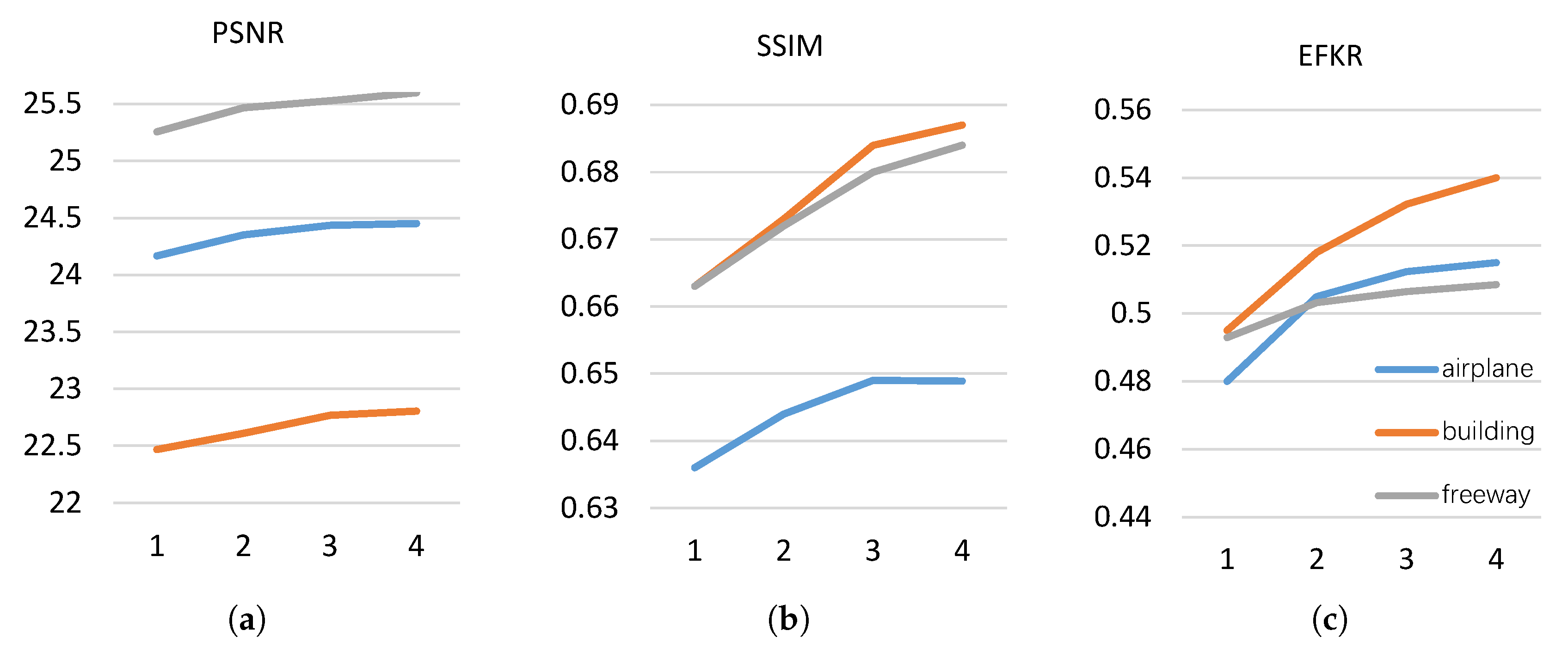
To select a proper scale, building, freeway, and airplane, three classes of test images are used to analyze. Figure 13 shows the testing results of networks with different scales. In the single-scale network, recurrent modules ConvLSTM are replaced by a convolution layer to keep the same number of convolution layers.

We can observe that as the scale increases, the values of the three evaluation metrics are all improved. It suggests that exploiting the multi-scale information can help with improving network performance. However, we can meanwhile find that the improvement is small while the scale is greater than 3. We thus choose s=3 in our network to balance the network performance and complexity.

5.2. Loss Function

The influence of loss function on network performance is also discussed in this paper. Instead of ${\mathcal{L}}_1$ loss, ${\mathcal{L}}_2$ loss function is used to train our MSR-net. ${\mathcal{L}}_2$ norm loss, also called Euclidean loss, is the most commonly used loss function in despeckling tasks. It is defined as:

$${\mathcal{L}}_2(\Theta )=\frac{1}{2N}\sum _{y=1}^W\sum _{x=1}^H{∥\phi \left(\mathbf{X}(x,y);\Theta \right)-\mathbf{C}(x,y)∥}_2^2$$

(14)

where $\Theta$ is the filter parameter that needs to be updated during the training process, $\mathbf{C}$ is the ground truth image without noise, $\mathbf{X}$ is the input image with speckle noise, and $\phi \left(·\right)$ is the output after despeckling. The purpose of training network is to minimize the cost. Smaller loss value suggests a smaller error between the network output and its corresponding ground truth.

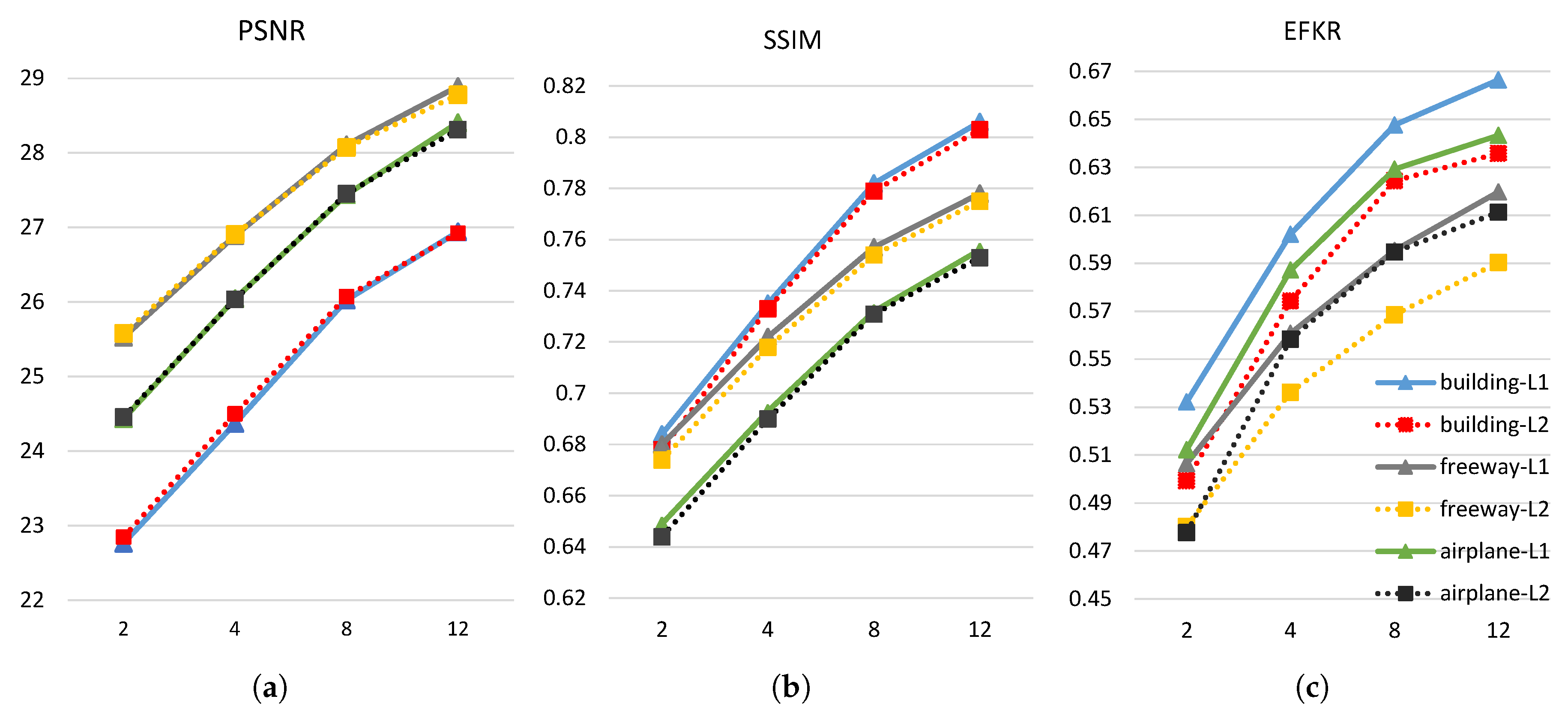
As shown in Figure 14, the network trained by ${\mathcal{L}}_2$ loss function is more likely to obtain a higher PSNR only for building images and the network trained by ${\mathcal{L}}_1$ loss function can obtain both slightly higher PSRN and SSIM with the other images. But for EFKR, the advantage of ${\mathcal{L}}_1$ loss is significant compared to ${\mathcal{L}}_2$ loss. Generally speaking, the ${\mathcal{L}}_1$ loss is more suitable to SAR despeckling task.

6. Conclusions

In summary, different from the existing despeckling network, MSR-net proposed in this paper adopts the coarse-to-fine structure and the convolutional long short-term memory unit that can obtain high-quality despeckling SAR images. During research, we find that the weights sharing strategy of convolutional kernels can reduce network parameters and training complexity, and the sub-pixel unit used in this work can reduce up-sampling complexity, improve network efficiency, and shorten the runtime of the network with respect to the transposed convolutional layer. Meanwhile, new design evaluation metrics EFKR and FPKR are introduced herein to evaluate the compatibility of the despeckling algorithms to the optical image processing algorithms. Experimental results show that our MSR-net has excellent despeckling ability and achieves the state-of-the-art results both for simulated and real SAR images with low computational costs, especially in low signal noise ratio cases. The adaptability of optical image processing algorithms to SAR images can be enhanced after despeckling in our network.

References

- Ranjani, J.J.; Thiruvengadam, S. Dual-tree complex wavelet transform based SAR despeckling using interscale dependence. IEEE Trans. Geosci. Remote Sens. 2010, 48, 2723–2731. [Google Scholar] [CrossRef]
- Ahishali, M.; Kiranyaz, S.; Ince, T.; Gabbouj, M. Dual and Single Polarized SAR Image Classification Using Compact Convolutional Neural Networks. Remote Sens. 2019, 11, 1340. [Google Scholar] [CrossRef]
- Jun, S.; Long, M.; Xiaoling, Z. Streaming BP for non-linear motion compensation SAR imaging based on GPU. IEEE J. Sel. Top. Appl. Earth Obs. Remote Sens. 2013, 6, 2035–2050. [Google Scholar] [CrossRef]
- Tang, X.; Zhang, X.; Shi, J.; Wei, S.; Tian, B. Ground Moving Target 2-D Velocity Estimation and Refocusing for Multichannel Maneuvering SAR with Fixed Acceleration. Sensors 2019, 19, 3695. [Google Scholar] [CrossRef]
- Lee, J.S.; Wen, J.H.; Ainsworth, T.L.; Chen, K.S.; Chen, A.J. Improved sigma filter for speckle filtering of SAR imagery. IEEE Trans. Geosci. Remote Sens. 2008, 47, 202–213. [Google Scholar]
- Yue, D.X.; Xu, F.; Jin, Y.Q. SAR despeckling neural network with logarithmic convolutional product model. Int. J. Remote Sens. 2018, 39, 7483–7505. [Google Scholar] [CrossRef]
- Xie, H.; Pierce, L.E.; Ulaby, F.T. Statistical properties of logarithmically transformed speckle. IEEE Trans. Geosci. Remote Sens. 2002, 40, 721–727. [Google Scholar] [CrossRef]
- Lee, J.S.; Hoppel, K.W.; Mango, S.A.; Miller, A.R. Intensity and phase statistics of multilook polarimetric and interferometric SAR imagery. IEEE Trans. Geosci. Remote Sens. 1994, 32, 1017–1028. [Google Scholar]
- Lattari, F.; Gonzalez Leon, B.; Asaro, F.; Rucci, A.; Prati, C.; Matteucci, M. Deep Learning for SAR Image Despeckling. Remote Sens. 2019, 11, 1532. [Google Scholar] [CrossRef]
- Lopes, A.; Touzi, R.; Nezry, E. Adaptive speckle filters and scene heterogeneity. IEEE Trans. Geosci. Remote Sens. 1990, 28, 992–1000. [Google Scholar] [CrossRef]
- Frost, V.S.; Stiles, J.A.; Shanmugan, K.S.; Holtzman, J.C. A model for radar images and its application to adaptive digital filtering of multiplicative noise. IEEE Trans. Pattern Anal. Mach. Intell. 1982, PAMI-4l, 157–166. [Google Scholar] [CrossRef]
- Kuan, D.T.; Sawchuk, A.A.; Strand, T.C.; Chavel, P. Adaptive noise smoothing filter for images with signal-dependent noise. IEEE Trans. Pattern Anal. Mach. Intell. 1985, PAMI-7, 165–177. [Google Scholar] [CrossRef]
- Lopes, A.; Nezry, E.; Touzi, R.; Laur, H. Structure detection and statistical adaptive speckle filtering in SAR images. Int. J. Remote Sens. 1993, 14, 1735–1758. [Google Scholar] [CrossRef]
- Kaur, L.; Gupta, S.; Chauhan, R. Image Denoising Using Wavelet Thresholding. ICVGIP Indian Conf. Comput. Vision Graph. Image Process. 2002, 2, 16–18. [Google Scholar]
- Cohen, A.; Daubechies, I.; Feauveau, J.C. Biorthogonal bases of compactly supported wavelets. Commun. Pure Appl. Math. 1992, 45, 485–560. [Google Scholar] [CrossRef]
- Donovan, G.C.; Geronimo, J.S.; Hardin, D.P.; Massopust, P.R. Construction of orthogonal wavelets using fractal interpolation functions. Siam J. Math. Anal. 1996, 27, 1158–1192. [Google Scholar] [CrossRef]
- Xie, H.; Pierce, L.E.; Ulaby, F.T. SAR speckle reduction using wavelet denoising and Markov random field modeling. IEEE Trans. Geosci. Remote Sens. 2002, 40, 2196–2212. [Google Scholar] [CrossRef] [Green Version]
- Candes, E.J.; Donoho, D.L. Curvelets: A Surprisingly Effective Nonadaptive Representation for Objects with Edges; Technical Report; Stanford University, Department of Statistics: Stanford, CA, USA, 2000. [Google Scholar]
- Meyer, F.G.; Coifman, R.R. Brushlets: A tool for directional image analysis and image compression. Appl. Comput. Harmon. Anal. 1997, 4, 147–187. [Google Scholar] [CrossRef]
- Do, M.N.; Vetterli, M. The contourlet transform: an efficient directional multiresolution image representation. IEEE Trans. Image Process. 2005, 14, 2091–2106. [Google Scholar] [CrossRef] [Green Version]
- Buades, A.; Coll, B.; Morel, J.M. A non-local algorithm for image denoising. In Proceedings of the 2005 IEEE Computer Society Conference on Computer Vision and Pattern Recognition (CVPR’05), San Diego, CA, USA, 20–25 June 2005; Volume 2, pp. 60–65. [Google Scholar]
- Parrilli, S.; Poderico, M.; Angelino, C.V.; Verdoliva, L. A nonlocal SAR image denoising algorithm based on LLMMSE wavelet shrinkage. IEEE Trans. Geosci. Remote Sens. 2011, 50, 606–616. [Google Scholar] [CrossRef]
- Deledalle, C.A.; Denis, L.; Tupin, F.; Reigber, A.; Jäger, M. NL-SAR: A unified nonlocal framework for resolution-preserving (Pol)(In) SAR denoising. IEEE Trans. Geosci. Remote Sens. 2014, 53, 2021–2038. [Google Scholar] [CrossRef]
- Kervrann, C.; Boulanger, J.; Coupé, P. Bayesian non-local means filter, image redundancy and adaptive dictionaries for noise removal. In Proceedings of the International Conference on Scale Space and Variational Methods in Computer Vision, Ischia, Italy, 30 May–2 June 2007; pp. 520–532. [Google Scholar]
- Wang, P.; Zhang, H.; Patel, V.M. SAR image despeckling using a convolutional neural network. IEEE Signal Process. Lett. 2017, 24, 1763–1767. [Google Scholar] [CrossRef]
- Bai, Y.C.; Zhang, S.; Chen, M.; Pu, Y.F.; Zhou, J.L. A Fractional Total Variational CNN Approach for SAR Image Despeckling. In Proceedings of the International Conference on Intelligent Computing, Bengaluru, India, 6 July 2018; pp. 431–442. [Google Scholar]
- Zhang, Q.; Yuan, Q.; Li, J.; Yang, Z.; Ma, X. Learning a dilated residual network for SAR image despeckling. Remote Sens. 2018, 10, 196. [Google Scholar] [CrossRef]
- Kaplan, L.M. Analysis of multiplicative speckle models for template-based SAR ATR. IEEE Trans. Aerosp. Electron. Syst. 2001, 37, 1424–1432. [Google Scholar] [CrossRef]
- Oliver, C.; Quegan, S. Understanding Synthetic Aperture Radar Images; SciTech Publishing: Noida, India, 2004. [Google Scholar]
- Wang, C.; Shi, J.; Yang, X.; Zhou, Y.; Wei, S.; Li, L.; Zhang, X. Geospatial Object Detection via Deconvolutional Region Proposal Network. IEEE J. Sel. Top. Appl. Earth Obs. Remote Sens. 2019, 12, 3014–3027. [Google Scholar] [CrossRef]
- Lecun, Y.; Bengio, Y.; Hinton, G. Deep learning. Nature 2015, 521, 436. [Google Scholar] [CrossRef]
- Xingjian, S.; Chen, Z.; Wang, H.; Yeung, D.Y.; Wong, W.K.; Woo, W.C. Convolutional LSTM network: A machine learning approach for precipitation nowcasting. In Advances in Neural Information Processing Systems; MIT Press: Cambridge, MA, USA, 2015; pp. 802–810. [Google Scholar]
- Hochreiter, S.; Schmidhuber, J. Long short-term memory. Neural Comput. 1997, 9, 1735–1780. [Google Scholar] [CrossRef]
- Chen, Q.; Koltun, V. Photographic image synthesis with cascaded refinement networks. In Proceedings of the IEEE International Conference on Computer Vision, Venice, Italy, 22–29 October 2017; pp. 1511–1520. [Google Scholar]
- Srivastava, R.K.; Greff, K.; Schmidhuber, J. Highway networks. arXiv 2015, arXiv:1505.00387. [Google Scholar]
- He, K.; Sun, J. Convolutional neural networks at constrained time cost. In Proceedings of the IEEE Conference on Computer Vision and Pattern Recognition, Santiago, Chile, 7–13 December 2015; pp. 5353–5360. [Google Scholar]
- He, K.; Zhang, X.; Ren, S.; Sun, J. Deep residual learning for image recognition. In Proceedings of the IEEE Conference on Computer Vision and Pattern Recognition, Las Vegas, NV, USA, 27–30 June 2016; pp. 770–778. [Google Scholar]
- Dumoulin, V.; Visin, F. A guide to convolution arithmetic for deep learning. arXiv 2016, arXiv:1603.07285. [Google Scholar]
- Long, J.; Shelhamer, E.; Darrell, T. Fully convolutional networks for semantic segmentation. In Proceedings of the IEEE Conference on Computer Vision and Pattern Recognition, Santiago, Chile, 7–13 December 2015; pp. 3431–3440. [Google Scholar]
- He, K.; Gkioxari, G.; Dollár, P.; Girshick, R. Mask r-cnn. In Proceedings of the IEEE International Conference on Computer Vision, Venice, Italy, 22–29 October 2017; pp. 2961–2969. [Google Scholar]
- DeTone, D.; Malisiewicz, T.; Rabinovich, A. Superpoint: Self-supervised interest point detection and description. In Proceedings of the IEEE Conference on Computer Vision and Pattern Recognition Workshops, Salt Lake City, UT, USA, 18–22 June 2018; pp. 224–236. [Google Scholar]
- Odena, A.; Dumoulin, V.; Olah, C. Deconvolution and checkerboard artifacts. Distill 2016, 1, e3. [Google Scholar] [CrossRef]
- Shi, W.; Caballero, J.; Huszár, F.; Totz, J.; Aitken, A.P.; Bishop, R.; Rueckert, D.; Wang, Z. Real-time single image and video super-resolution using an efficient sub-pixel convolutional neural network. In Proceedings of the IEEE Conference on Computer Vision and Pattern Recognition, Las Vegas, NV, USA, 26 June–1 July 2016; pp. 1874–1883. [Google Scholar]
- Goodman, J.W. Statistical properties of laser speckle patterns. In Laser Speckle and Related Phenomena; Springer: Berlin/Heidelberg, Germany, 1975; pp. 9–75. [Google Scholar]
- Wang, Z.; Bovik, A.C.; Sheikh, H.R.; Simoncelli, E.P. Image quality assessment: from error visibility to structural similarity. IEEE Trans. Image Process. 2004, 13, 600–612. [Google Scholar] [CrossRef] [PubMed]
- Anfinsen, S.N.; Doulgeris, A.P.; Eltoft, T. Estimation of the equivalent number of looks in polarimetric synthetic aperture radar imagery. IEEE Trans. Geosci. Remote Sens. 2009, 47, 3795–3809. [Google Scholar] [CrossRef]
- Sobel, I. History and definition of the sobell operator. Retrieved World Wide Web. 2014. Available online: Available online: https://www.researchgate.net/publication/239398674 (accessed on 23 October 2019).
- Bao, P.; Zhang, L.; Wu, X. Canny edge detection enhancement by scale multiplication. IEEE Trans. Pattern Anal. Mach. Intell. 2005, 27, 1485–1490. [Google Scholar] [CrossRef] [PubMed] [Green Version]
- Dim, J.R.; Takamura, T. Alternative approach for satellite cloud classification: edge gradient application. Adv. Meteorol. 2013, 2013, 584816. [Google Scholar] [CrossRef]
- Davis, L.S. A survey of edge detection techniques. Comput. Graph. Image Process. 1975, 4, 248–270. [Google Scholar] [CrossRef]
- Tareen, S.A.K.; Saleem, Z. A comparative analysis of sift, surf, kaze, akaze, orb, and brisk. In Proceedings of the IEEE 2018 International Conference on Computing, Mathematics and Engineering Technologies (iCoMET), Sukkur, Pakistan, 3–4 March 2018; pp. 1–10. [Google Scholar]
- Yang, Y.; Newsam, S. Bag-of-visual-words and spatial extensions for land-use classification. In Proceedings of the 18th SIGSPATIAL International Conference on Advances in Geographic Information Systems, San Jose, CA, USA, 2–5 November 2010; pp. 270–279. [Google Scholar]
- Couturier, R.; Perrot, G.; Salomon, M. Image Denoising Using a Deep Encoder-Decoder Network with Skip Connections. In Proceedings of the International Conference on Neural Information Processing, Siem Reap, Cambodia, 13–16 December 2018; pp. 554–565. [Google Scholar]
- He, K.; Zhang, X.; Ren, S.; Sun, J. Delving deep into rectifiers: Surpassing human-level performance on imagenet classification. In Proceedings of the IEEE International Conference on Computer Vision, Santiago, Chile, 7–13 December 2015; pp. 1026–1034. [Google Scholar]
- Kingma, D.P.; Ba, J. Adam: A method for stochastic optimization. arXiv 2014, arXiv:1412.6980. [Google Scholar]
- Kaplan, A.; Avraham, T.; Lindenbaum, M. Interpreting the ratio criterion for matching SIFT descriptors. In Proceedings of the European Conference on Computer Vision, Amsterdam, The Netherlands, 8–16 October 2016; pp. 697–712. [Google Scholar]
Figure 1.
Inner structure of convolutional long short-term memory (ConvLSTM) [32].
Figure 2.
The architecture of Multi-scale Recurrent. The yellow arrow denotes up-sampling by one time.
Figure 3.
Architecture of Single Scale Modle
Figure 4.
Diagram of checkerboard artifacts. (a) original image without noise; (b) despeckling image with checkerboard artifacts caused by transposed convolution.
Figure 5.
The sub-pixel convolutional operation on the input feature maps with an upscaling factor of r = 2, channel c = 1.
Figure 6.
Edge detection results. Images from left to right correspond to a clean image, an image with speckle noise, and image after despeckling.
Figure 7.
Part of the sample images used to train the network.
Figure 8.
Test results on images of airplanes with four levels of noise. The noise level from left to right is L = 2, L = 4, L = 8, and L = 12. (a) Speckled image (b) SAR-BM3D (Block-Matching and 3D filtering) (c) image despeckling convolutional neural network (ID-CNN) (d) RED-Net (e) multi-scale recurrent network (MSR-net).
Figure 9.
Test results on images of buildings with four levels of noise. The noise level from left to right is L = 2, L = 4, L = 8, and L = 12. (a) Speckled image (b) SAR-BM3D (c) ID-CNN (d) RED-Net (e) MSR-net.
Figure 10.
Test results of Real SAR images (RADARSAT-2). (a) Original, (b) SAR-BM3D, (c) ID-CNN, (d) RED-Net, (e) single scale network (SS-net), (f) MSR-net.
Figure 11.
Test results of Real SAR images (RADARSAT-2). (a) Original, (b) SAR-BM3D, (c) ID-CNN, (d) RED-Net, (e) SS-net, (f) MSR-net.
Figure 12.
Search results of feature point pairs for synthetic aperture radar (SAR) image before and after despeckling.
Figure 13.
Test results of proposed network with scale 1, 2, 3, 4 when nosie level L = 2.
Figure 14.
Evaluation index (PSNR, SSIM, and EFKR) values of MSR-net with L1 and L2 Loss.