In-Field Detection of Yellow Rust in Wheat on the Ground Canopy and UAV Scale

1
INRES-Plant Diseases and Plant Protection, University of Bonn, Nussallee 9, D-53115 Bonn, Germany
2
Institute of Sugar Beet Research (IfZ), Holtenser Landstraße 77, D-37079 Göttingen, Germany
*
Author to whom correspondence should be addressed.
Remote Sens. 2019, 11(21), 2495; https://0-doi-org.brum.beds.ac.uk/10.3390/rs11212495
Submission received: 26 September 2019
/
Revised: 22 October 2019
/
Accepted: 23 October 2019
/
Published: 25 October 2019
(This article belongs to the Special Issue Remote Sensing in Agriculture: State-of-the-Art)
Abstract
:The application of hyperspectral imaging technology for plant disease detection in the field is still challenging. Existing equipment and analysis algorithms are adapted to highly controlled environmental conditions in the laboratory. However, only real time information from the field scale is able to guide plant protection measures and to optimize the use of resources. At the field scale, many parameters such as the optimal measurement distance, informative feature sets, and suitable algorithms have not been investigated. In this study, the hyperspectral detection and quantification of yellow rust in wheat was evaluated using two measurement platforms: a ground-based vehicle and an unmanned aerial vehicle (UAV). Different disease development stages and disease severities were provided in a plot-based field experiment. Measurements were performed weekly during the vegetation period. Data analysis was performed by three prediction algorithms with a focus on the selection of optimal feature sets. In this context, the across-scale application of optimized feature sets, an approach of information transfer between scales, was also evaluated. Relevant aspects for an on-line disease assessment in the field integrating affordable sensor technology, sensor spatial resolution, compact analysis models, and fast evaluation have been outlined and reflected upon. For the first time, a hyperspectral imaging observation experiment of a plant disease was comparatively performed at two scales, ground canopy and UAV.
1. Introduction
Today’s demands of agricultural cropping systems are high. Agroecosystems have to be highly productive, while the undesirable impact on the environment has to be as low as possible. Resource-conserving methods with a minimum of chemical input are in favor. One vision able to approximate this goal is the use site-specific cropping measures. Site-specific management has the potential to lead to a higher or constant productivity with a constant or reduced input of resources [1]. One group of for site-specific applications are plant protection measures [2].
The spatial occurrence of plant diseases in the field, especially in the early season, is often heterogeneous, while in most cases, plant protection compounds are applied homogeneously onto the crop. This spatial heterogeneity of disease occurrence might lead to diverse fungicide demands that are often not considered. Many diseases first occur in patches before they start spreading in the field. One approach for a site-specific application of plant protection measures might be the application of fungicides to patches of disease occurrence [3,4,5]. This could prevent or stop disease spreading without applying a fungicide to the whole field [1].
Spectral sensors might be tools able to contribute to site-specific disease management [6,7]. Spectral sensors measure the light reflected from the crop canopy [1]. During pathogen attack and disease development on the crop leaf, diseases establish a spectral fingerprint in the reflected leaf signature [8,9,10]. These shifts of the signature can be detected using spectral sensors, particularly in the electromagnetic spectrum from 400–2500 nm [11]. Spectral sensors can be divided into hyperspectral and multispectral sensors, depending on their spectral resolution. The number and width of measured wavebands mainly characterize the spectral resolution [11].
Non-imaging hyperspectral sensors average the spectral information over a certain area, while imaging sensors contain the spectral information for each pixel [7]. Hyperspectral imaging sensors (HSIs) provide spectral information in a spatial resolution. Multispectral sensors typically cover the RGB range with an additional NIR band. These sensors are less cost-intensive and the generated data are less complex, but do not cover the broad spectral range like a hyperspectral sensor.
Spectral sensors have been applied on different scales [12]. For field approaches, a hyperspectral camera can be mounted to a ground based vehicle or to a UAV [1,3,11,13]. Depending on the interrogation and measuring setup, each scale can have advantages and disadvantages. On the ground scale, it is possible to detect small features of a few mm through high resolution on close range, while the throughput on the UAV scale is much higher, with still higher resolution compared to satellite imagery [5,14,15,16]. For field applications of spectral sensors, depending on the scale, the resolution or the measurement time can become a limiting factor. Most field applications for disease detection focused on the calculation of vegetation indices (VIs) [17,18,19] using multispectral sensors. VIs are developed by accounting certain band ratios to highlight one factor and reduce the impact of another factor [20]. Depending on the wavelength, these indices can be indicators for crop vitality, general crop stress, pigment content, or a specific plant disease [18,21]. Few works have demonstrated an approach for disease detection using imaging hyperspectral sensors under field conditions [10]. This might be because spectral measurements under field conditions are challenging and the complexity of hyperspectral data is higher than multispectral data [1]. The features of multispectral sensors might result in lower image acquisition durations and lower susceptibility to environmental factors during measurements. The image quality of field data in general is influenced by various factors. Beside suitable weather conditions, the field crop species and the disease symptom type are of high relevance for successful measurements. The leaf architecture and disease occurrence on the plant mainly determine the detectability of the disease. Disease presence on lower plant and leaf levels results in a decreased reflected signal. Disturbing weather conditions such as wind and rain can easily obscure spectral images obtained in the field. One elusive and eminently important factor is the illumination. Changing illumination conditions over time, caused by clouds or solar altitude, can lead to uninterpretable data, because spectra of different images cannot be compared with one another anymore [1,3,22]. The detection of diseases on different leaf levels is also challenging because of inhomogeneous illumination conditions through the leaf altitude in the crop stand and upper leaves that cast shadow. These leaves might also be in different developmental stages, and a senescent leaf has to be differentiated from a healthy green or a diseased leaf. The leaf angle to the camera influences the spectral signal. Not least, the image quality is essentially determined by the spatial resolution of the sensor system used. Small symptoms of a disease can only be visualized when the spatial resolution in combination with the measurement distance is appropriate for the desired data quality.
So far, various field measurements on the ground canopy scale of cereal crops have focused on the detection of biotrophic diseases such as yellow rust [3,10,13,23,24,25], brown rust [18,26], and powdery mildew of wheat [19]. This might be due to the fact that biotrophic diseases are more likely to appear on the upper leaf layers because of wind distribution and a preference for fresh and healthy leaf tissue [27]. Necrotrophic diseases are most severe on lower leaf levels, and therefore more difficult to detect with remote sensors. A detection and quantification of septoria tritici blotch with a hyperspectral radiometer has been demonstrated in the field [28].
The analysis and interpretation of sensor data is crucial for future implementation. Algorithms from machine and deep learning, in combination with suitable sensors and measurement platforms are promising techniques. These methods are particularly able to cope with the number of wavebands provided in hyperspectral data, and can be used for the detection of plant diseases [7,29,30,31,32].
This work presents a new approach for field trial studies using innovative and machine learning for a pixel wise detection of crop diseases. A winter wheat trial was conducted in the vegetation period of 2018. The crop was infected with Puccinia striiformis, the causal agent of yellow rust (YR). Weekly hyperspectral measurements were performed on the ground-canopy and the UAV scale to monitor the spectral dynamic of crop stands during the vegetation period. Measurements were performed using a mobile field platform with a distance of 50 cm to the crop canopy and with a UAV drone at 20 m height over the plots to work on and compare different scales. Hyperspectral images were captured using a line scanner attached to a linear stage in a measurement booth and a frame-based hyperspectral camera for UAV applications. Field data were preprocessed and normalized, and then analyzed using the supervised classification methods spectral angle mapper (SAM) and support vector machine (SVM) to detect yellow rust of wheat. Additionally, a feature selection was performed on the hyperspectral data to verify the potential for a waveband reduction from hyperspectral to multispectral data for disease detection.
2. Materials and Methods
2.1. Field Trial Layout
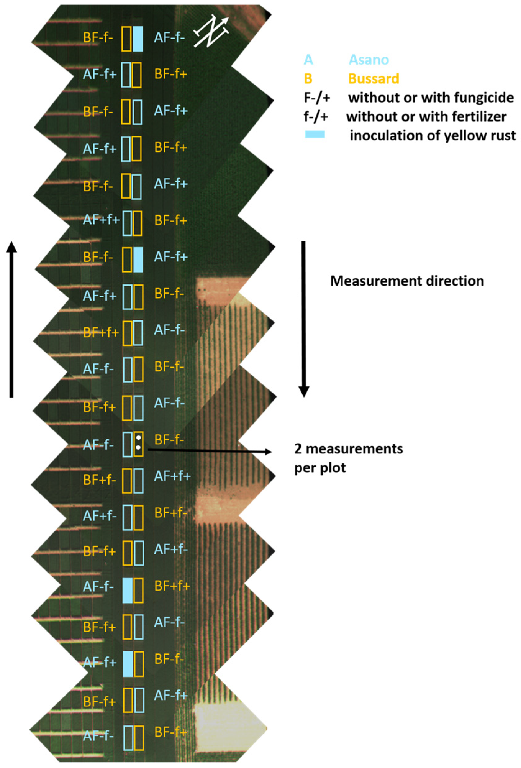
In the vegetation period 2017/2018, a field trial with winter wheat was conducted at trial station Campus Klein-Altendorf 50°37′31.00′’N, 6°59′20.54′’E (Rheinbach, Germany). In 2016/2017, a first field trial was performed to specify the measuring setup and routine (data are not shown). The cultivars JB Asano (Limagrain GmbH, Edemissen, Germany) and Bussard (KWS SAAT SE, Einbeck, Germany) were sown on 26.10.2017 with 320 kernels/m². Field emergence was on 14th November 2017, while harvest took place on 24.07.2018. JB Asano was chosen because of its susceptibility to YR. The field trial was designed in 10 treatments per cultivar with two repetitions, resulting in 40 plots (plot size: 3 × 7 m). The plot design was randomized within each cultivar. With a change of the cultivar after each plot, the direct proximity of plots with the same cultivar was avoided. This was designed to arrange the field trial into two long rows of plots with cultivars alternating one after another in 20 plots per repetition (Figure 1). The treatments within one cultivar were randomized. Two fertilizer intensities (160 kg N/ha and 30 kg N/ha) were applied per cultivar. For cultivar Asano, two treatments were used for additional inoculation with YR. The whole field trial was aligned from northwest to southeast.
2.1.1. Inoculations
Additional inoculations of Puccinia striiformis were performed in April and May (25 April 2019; 12 May 2019). To establish high disease infections, the inoculations were repeatedly performed by applying a spore suspension to the plants immediately after rainfall incidences. Inoculations were timed to forecasted infection risks after the xarvio field manager (BASF Digital Farming GmbH, Münster, Germany). The spore suspension was applied with a garden pump sprayer and contained 8 × 10⁴ spores/mL. Two liters of spore suspension were homogeneously applied over one plot.
2.1.2. Visual Disease Ratings
Visual disease ratings were performed weekly from calendar week 17–23. One plot was rated two times at the same locations where hyperspectral measurements took place. Disease incidence was assessed by the eye of a human rater. The diseased leaf area (%) was rated on 15 leaves per leaf level. Additionally, the growing stage and the visible leaf area of each leaf level in the hyperspectral image (from top view) was ascertained.
2.1.3. Crop Stand and Disease Development
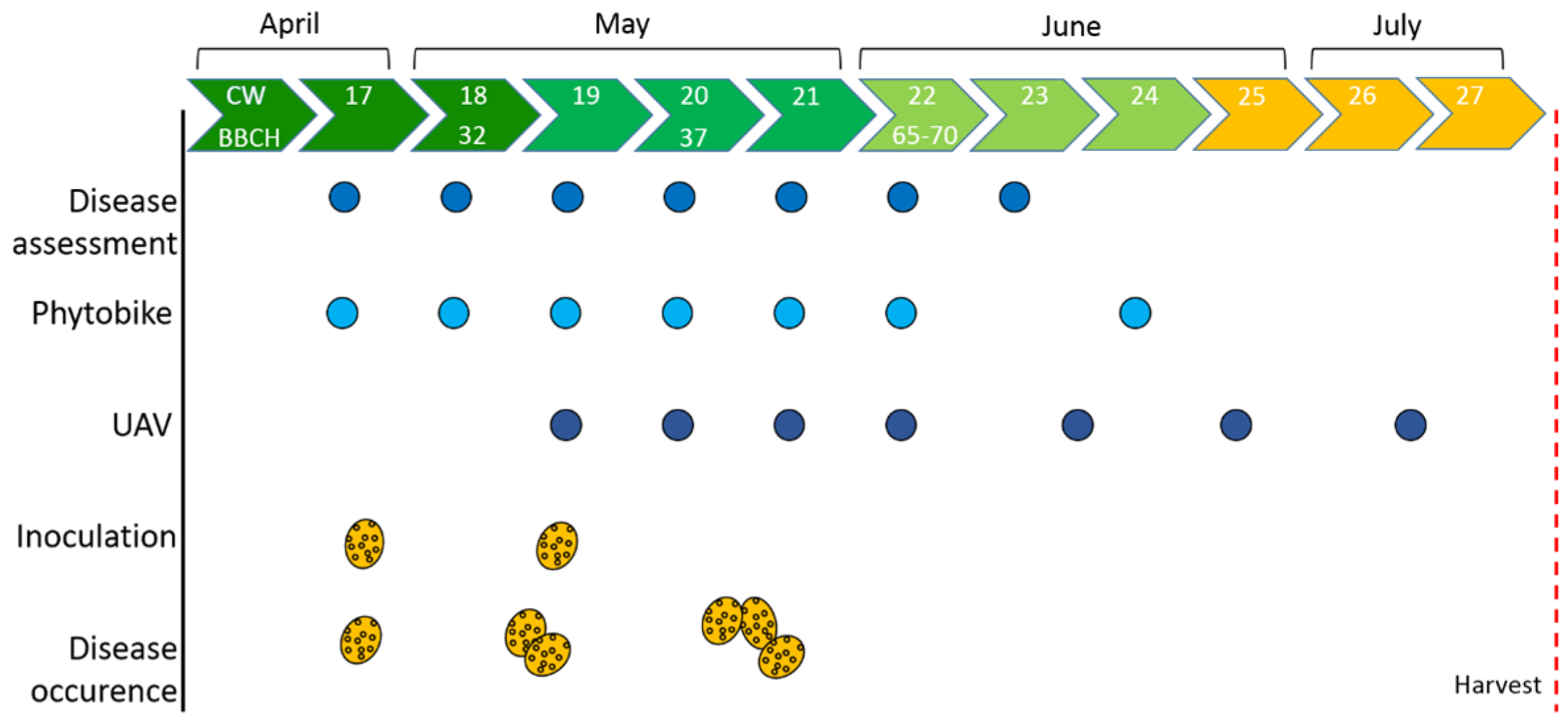
The vegetation in 2018 started late in March and was denoted by a drought that especially affected the length of the growing season and led to an early harvest in July (Figure 2). Septoria tritici blotch, tan spot, and powdery mildew were insignificant throughout the growing season. YR could establish a significant infection on cultivar Asano, and measurements were not aggravated due to mixed infections. The first YR symptoms were found in mid of April and were based on natural infection incidences. Until the beginning of May (BBCH 31), a serious increase of YR was rated. Warm days and cold nights seemed to favor infection incidences through dew formation. Until the middle of May (BBCH 37-39), YR was the dominating disease.
2.2. Measurement Platforms
2.2.1. Field Platform Phytobike
The measurement platform, based on a square steel construction with four wheels and provided by Forschungszentrum Jülich (Jülich, Germany), covered a 3 m wide experimental plot (Figure 3). Sensors for reflectance characteristics, localization systems, power supply, and control of the sensors via a control laptop were mounted to the steel frame. All sensors were variable in height by a moveable aluminum profile construction. In this way, the sensor platform could be adapted to the growth stages of the plants and a constant distance between sensors and crop canopy was enabled. With a weight of around 150 kg, the construction approached the limit of the platforms without steering, and could still be moved by the physical strength of two people.
As a hyperspectral sensor, the Specim V10E line camera (Specim Oy, Oulu, Finland) was used. The motion required for the Specim V10E camera was realized by a linear stage (Velmex, Bloomfield, USA). Measurements were triggered via the control computer, allowing a flexible reaction to changing light situations by an adapted integration time. The Specim V10E camera measured the electromagnetic spectrum in a range from 400 to 1000 nm with a spectral resolution of 2.73 nm. Sunlight was used as a natural light source. A canvas measuring cabin was constructed to avoid shadows cast by the sensors and equipment of the Phytobike.
2.2.2. UAV Measurements
The UAV allowed overview images of whole experiments or at least of parts of the experiment to be collected. Recent technologies have enabled hyperspectral imaging at UAV scale. We combined a UAV DJI Matrice 600 (Da-Jiang Innovations Science and Technology Co., Shenzen, China) with a Rikola hyperspectral camera (Senop Oy, Oulu, Finland) (Figure 3). The Rikola camera measured the reflected light in a range from 500 to 900 nm. The measured wavebands were selectable and spectral resolution was set to 7 nm using 55 wavebands. With flight times of around 20 min, the whole experiment was captured within one battery capacity. For plot observations, a 20 m flight height was selected and the UAV hovered over each plot center for a duration of 10 s. Sunlight was used as a natural light source.
2.3. Data Preprocessing
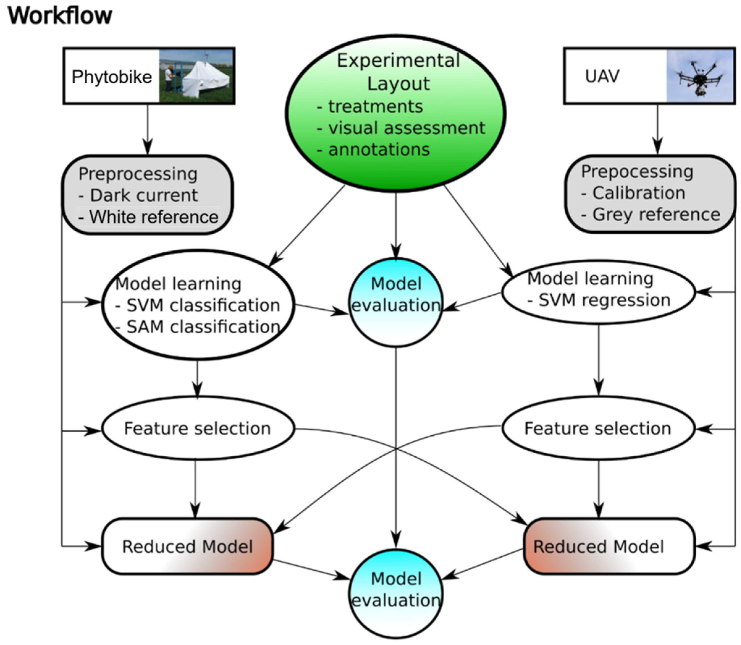
This study focused on the information about relevant wavebands as the central outcome. We used a data flow to assess the ability to transfer this information between observation scales (Figure 4). We built two data sets for yellow rust prediction—a classification data set on field scale and a regression data set on UAV scale. Multiple prediction models and feature selection results were derived. In the final step, models were optimized using the selected features, and feature selection information was also exchanged. The resulting four classification models with selected features, two on the field scale (features selected on the field scale and on the UAV scale) and two on the UAV scale (features selected on the field scale and on the UAV scale), were evaluated. This allowed the values of feature selection and, more specifically, the values of feature information obtained at a different observational scales to be evaluated.
2.3.1. Spectral Preprocessing
The derivation of the physical surface property reflectance from observed intensity values is an essential part of hyperspectral image processing. The normalization procedure has to be adapted to the measurement platform and is based on a spectral reference panel with a known homogeneous reflectance in the observed wavelengths. At all scales, the following equation was applied to calculate the reflectance R from the observation Im, reference Imref, and the corresponding dark currents DCIm and DCref. In the field, the additional DCref was omitted for practical reasons.
On the ground canopy scale, a 50% spectral reference panel was measured within each image of the line scanner. A separate dark current was observed for the Specim V10E camera before every image. For practical reasons, UAV flight sequences were started with the acquisition of a single dark current, and one image of the reference panel immediately before and after flying the frame-based Rikola camera over the wheat plots. Image quality always suffers from motion of the object to be measured or motion of the sensor. To avoid this, images were taken in conditions as calm as possible on the ground canopy scale. The Rikola camera was hovered for at least 10 images over the reference panel to ensure that image quality was sufficient for data normalization. The use of cross-sensor normalization, e.g., by using a separate spectrometer that continuously logs the incoming light intensity, was tested but was not successful due to a deviating response characteristic between the different sensors.
To remove high frequency noise at the spectral border regions of the Specim V10e, the bands 1–20 (400–450 nm) and 181–211 (910–1000 nm) were excluded from further analysis, resulting in 161 used spectral bands. In addition, a Savitzky–Golay filter using 15 centered points and a polynomial of degree 3 smoothed the data of the Specim V10e.
2.3.2. Data Normalization
Plant geometry can present severe distortions due to varying leaf angles, leaf distances to the camera, and specular reflections on particular parts of the leaves. To compare the reflectance characteristics, omitting the additive and multiplicative factors, the standard normal variate (SNV) has been developed [33]. It is able to remove scaling factors due to varying distance or leaf angle, as well as additional factors like specular reflection, e.g., on leaf tips. The normalization was performed on both the ground canopy and field data. The SNV representation was calculated per spectrum S and focuses the shape of the spectral curve:
2.4. Prediction Algorithms
Multiple algorithms can perform predicting a class or continuous value based on features of a sample. In general, they use a vector representation as input. In this study, the classifiers spectral angle mapper (SAM) and support vector machine (SVM), as well as the regression algorithm—support vector regression (SVR)—were applied to the ground canopy data (taken with the phytobike). To train and evaluate the models, four images of one measuring day were annotated to be used as training data and four images were annotated to be used as test data. The number of annotated pixels differed in the different images due to natural heterogeneity in the crop stand. Pixel numbers were at least several thousand for each class, up to several hundred thousand pixels for all classes in one image. Based on the huge number of annotated pixels, models were trained on a subsampled data set, to make them trainable and to rebalance the classes. With the exception of the water class, all classes were trained with 1000 samples per class after subsampling of training data. The SAM was used because it has been described in the literature to work resiliently under inhomogeneous light conditions [34]. The development of the classification model was easy and fast. The SVM was used because, in theory, it is trained on the whole data set and considers the spectrum of each pixel as training data. Vegetation indices (VIs) were used because various published works have focused on VIs as tool for disease detection. VIs can be seen as established representatives for optical measurements of plant parameters. The models were trained using three data representations: full spectra, SNV normalization, and 20 spectral VIs. The results were compared to a SAM that represented the base line accuracy. The comparison was performed on the YR test data from 23 May 2018. The evaluation of different feature representations showed a small advantage of SNV normalizations, whereas it was treated as standard representation in the following. As performance measures, we applied the overall accuracy using six classes for the model, combining the background and the old leaves/straw class. Furthermore, we evaluated the F1 score (Table 1) for the class disease, providing a homogenized combination of precision and recall. The F1 score declares the number of pixels of one class that are correctly classified into this class after the formula 2 × (precision × recall) ÷ (precision + recall)). The two performance measures corresponded in tendency; however, the F1 score decreased faster as the large number of background pixels stabilized the overall accuracy.
2.4.1. Spectral Angle Mapper
The SAM is a prediction algorithm developed for the efficient classification of high- dimensional spectral data. The assignment uses the angle between the spectra to classify and reference spectra, treating a spectrum as high-dimensional vector [34]. The spectrum to be classified was assigned to the reference spectrum/class with the smallest angular distance. In addition, a threshold prohibited the assignment of spectra with a large angular distance.
2.4.2. Support Vector Algorithms
The SVM andSVR are established machine learning methods that have been proven to deal well in situations with many features but a very limited number of samples [35]. This is a common situation in hyperspectral data analysis, and following it is a suitable approach for hyperspectral remote sensing as well as close range imaging. A critical point for the application of SVM and SVR is the selection of the hyper parameters Cost C, kernel parameter γ (SVM) or C, and complexity control ν (ν-SVR). They were selected by grid search combined with a cross validation. Grid points were for C, for ν and for n. The optimization algorithm was the sequential minimal optimization SMO, and LIBSVM 3.18 with Matlab was used for as implementation [36].
2.5. Vegetation Indices
On hyperspectral images of ground canopy data, 20 VIs were tested to visualize crop heterogeneity and to detect yellow rust in the field. The composition was used because it has previously been successfully tested as an indicator for crop vitality [37]. The composition of VIs was chosen according to Behmann et al. [37]. Due to the limitation of available bands of the Rikola camera, only 16 VIs were used for UAV data and the ARVI, mRESR, mRENDVI, and SIPI were excluded.
2.6. Model Evaluation
To compare the performance of the different models on the respective data sets, different measures were applied depending on the model type. All measures were calculated on a test set that was not used in training. For classification models that determined the discrete classes y as a function f(X) of the data X, the accuracy was defined as the percentage of correctly classified data points. The F1 score, in contrast, was based on the precision and recall of each class. In regression tasks with continuous target variables, the coefficient of determination R², correlation, and root mean square error (RMSE) were applied. Due to the limited number of data, we applied leave-one-out cross validation to generate the test predictions. This procedure learns a model on the whole data set except for one sample. This was repeated for all samples in the data set.
2.7. Feature Selection
There are multiple approaches for feature selection, feature subset selection, and feature weighting. Filter approaches like Relief are very fast and provide a weight for each feature. In contrast, wrapper approaches have the big advantage of dealing well with high levels of redundancy and selecting the best subset with minimal size [38]. A major drawback is the high computational load. Feature selection at all scales (on ground-canopy and UAV images) was performed using a wrapper approach comprising a SVM or SVR, respectively. A sequential forward feature selection (Statistics Toolbox, Matlab2013a) was used, and the called criterion function minimizing the prediction error was implemented based on LIBSVM 3.18. For the SVM, the accuracy was maximized and for the SVR, the RMSE was minimized. Due to the limited number of samples in the UAV data set, a leave-one-out cross-validation was performed to generate the test predictions to calculate the criterion.
2.8. Spatial Resolution as a Key Parameter for Disease Detection
Besides the relevant wavelengths, the required spatial resolution or ground sampling distance (GSD) is highly important for the definition of a sensor capable of detecting different wheat diseases in the field. Based on the test and training data sets, simulations were performed where the test data were extracted from subsampled spectra by a factor of 2, 10, 20, and 100. A knn and an aggressive subsampling approach were compared to visualize the effects of different annotation strategies on the F1 score for the detection of YR.
3. Results and Discussion
3.1. Supervised Classification of Hyperspectral Pixels at the Ground Canopy Scale
One approach used to analyze hyperspectral data on the field scale is the pixel-wise classification into usual pixel (background, straw, healthy leaf tissue) and in disease specific symptoms. In the field experiment 2018, YR had a significant disease severity and classifiers for this disease were derived.
The use of 16 VIs reached a reasonable but not competitive performance. However, it has to be noted that we compared 161 features to 16, meaning a significant reduction in dimensionality. The results can be integrated in a later discussion of the various feature sets obtained by feature selection.
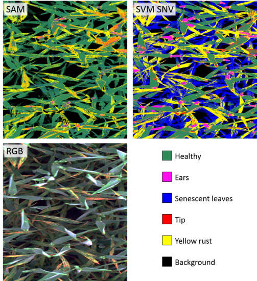
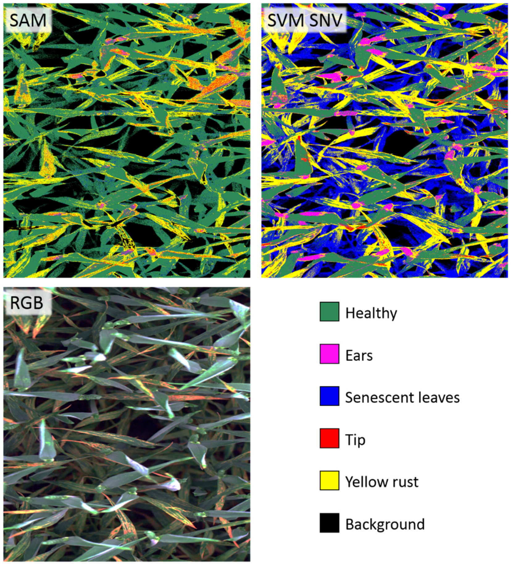
Based on these results, SVM SNV (Table 1) was selected as most appropriate approach. A visual comparison of the SAM results and the SVM SNV result is shown in Figure 5. Significant differences were apparent. The SVM detected many more senescent leaves, e.g., all leaves from the lower leaf levels, whereas the SAM assigned these to the background or the healthy leaves. The SVM was more sensitive for ear detection, which caused major problems in the SAM image, where they were partly assigned to YR. Overall, both approaches were sensitive to YR, but the SVM was much more accurate in the very bright image parts as well as the darker background parts, while the class YR was overrepresented in the SAM classification. The visually most significant aspect was the large number of blue pixels in the visualization of the SVM result. YR disease was present at all leaf levels and led to early senescence in lower leaf levels.
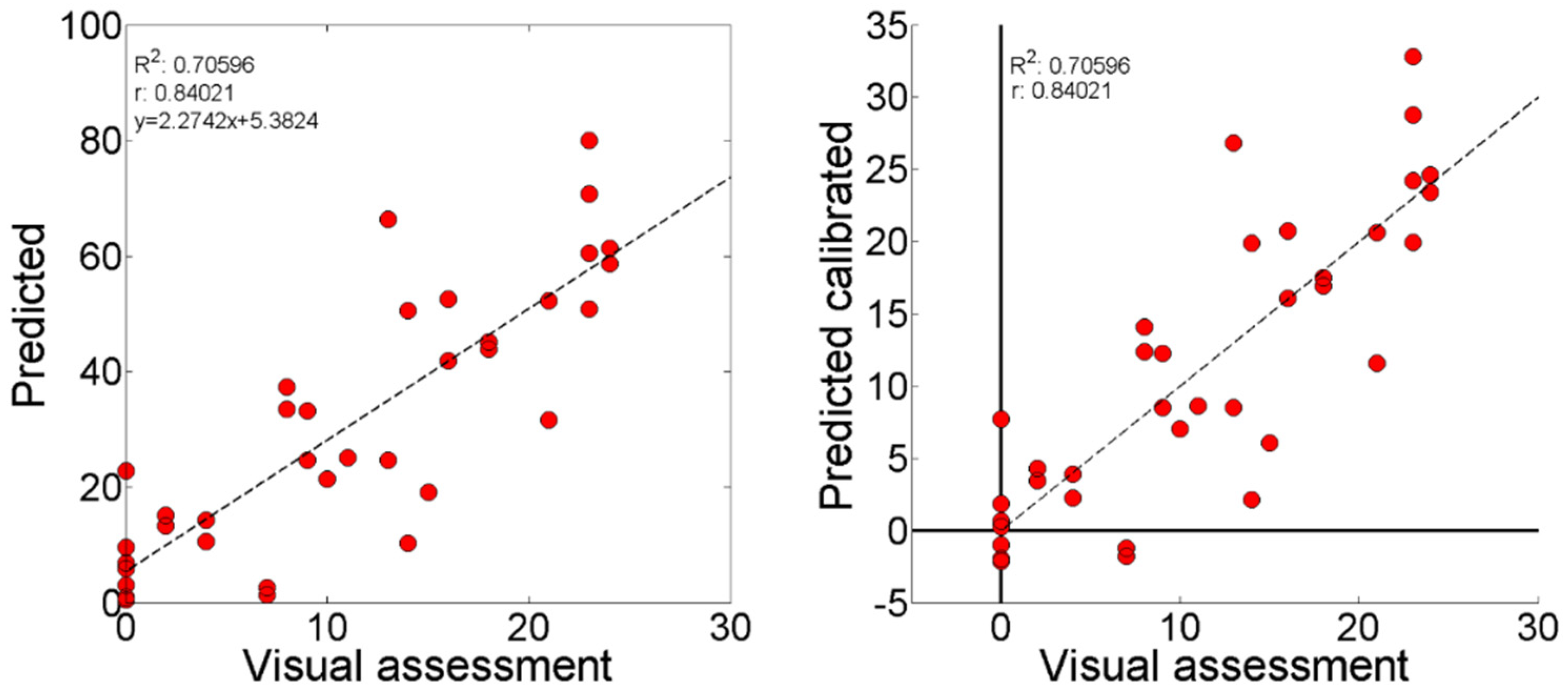
The classification models were validated via two approaches: (1) pixel-wise classification of the hold-out test data set consisting of manually annotated pixels of new images of separate plots, and (2) prediction of pixel classes of all images obtained on a respective day and comparing the total % disease class from all plant pixels to the visual assessment done by the expert (Figure 6). Approach 1 resulted in a confusion matrix allowing the calculation of multiple performance measures such as the overall accuracy, the sensitivity, and the recall, whereas Approach 2 provided the R²value, correlation coefficient, and a regression plot. Table 1 shows the overall accuracy and the F1 score for the different classification methods.
Presumably, due to light reflections and transmission or a deviating weighting of the different canopy levels, the SVM prediction overestimated the ratio of diseased pixels. To compensate for this, a linear regression model was applied. However, deviations between the predicted disease severity and the visual assessment could have various reasons, e.g., the section of the plot observed by the sensor did not represent the true status that was evaluated by the visual assessment. The viewing angle produced a variable composition of different leafs and leaf layers in the field of view of the human and the sensors. Furthermore, the visibility of the lower leaf levels was low for imaging system from the top, and more accurate if the human rater could go deep into the crop stand for individual leaf disease rating. Further points are that the visual assessment produced a single value averaging the affected leaf area. From repeated disease assessments with multiple experts, different deviations have been observed depending on the literature [39,40]. The method of disease detection is subjective to the individuals performing the assessment. Another prime factor for deviations and classification inaccuracies is the biological heterogeneity. This has to be considered as highly dynamic within one field, one plot, and one location, and even on different leaf layers and single leaves. The biological heterogeneity can be affected by many factors, e.g., the leaf color and status, stem elongation (distance of leaf layers), the density of the canopy, and other biological growth processes.
3.2. Evaluation of Hyperspectral UAV Observations Using a Filter-System Hyperspectral Camera
To characterize the reflectance characteristics of the field plots, the spectra of the central 4 × 2 m of each plot were averaged. Intra-plot variations were neglected. Multiple traits were predicted with reasonable accuracy based on SVM and SVR analysis of the 55 recorded bands from 500–900 nm. Table 2 shows the obtained performance parameters based on a SNV representation and the integration of all 55 bands.
Using the SVR approach, a prediction of the disease severity in percent was possible with reasonable accuracy (Figure 7). The interpretation of this result has to take into account that a value from the visual assessment might not represent the average plot value because diseases may occur at zoned locations in the plot, and assessment locations may or may not be in these spots.
3.3. Selection of Relevant Features at Different Scales
One of the main motivations for the application of hyperspectral imaging technology is the potential to find the most relevant wavelength for a specific task, and to subsequently design a specific sensor. Reference [41] showed that specific wavelengths might be useful to identify certain leaf diseases in sugar beet. In wheat, VIs have been described that are capable of detecting brown rust [18]. This shows that a selection of specific wavelengths can be specific for one disease. We applied the introduced technique to the data sets on the ground-canopy and UAV scale and derived important wavelength for the detection of disease symptoms as well as the prediction of disease severity.
3.3.2. Ground Scale
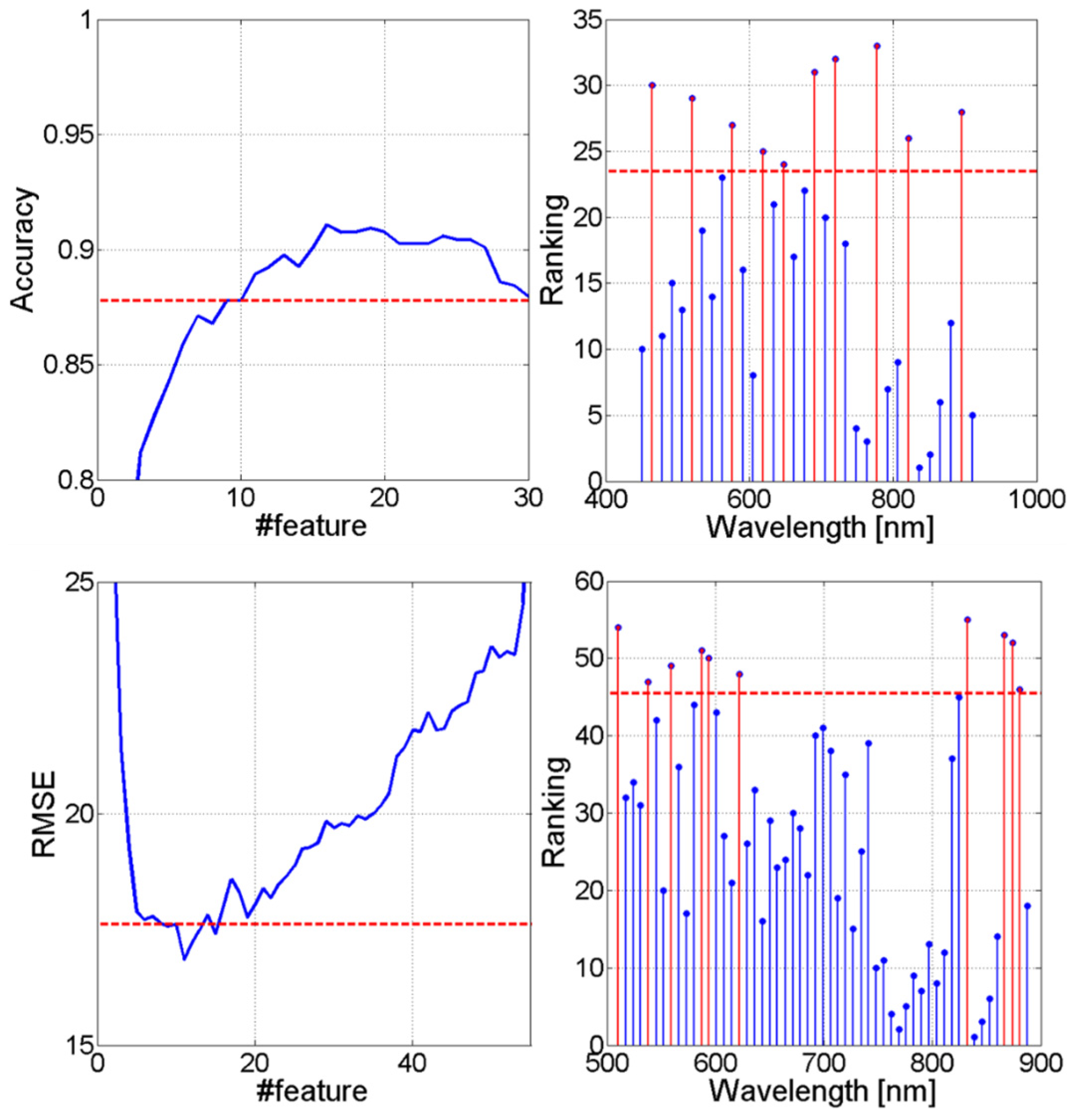
Feature selection on the field scale was performed for the detection of YR. The models were trained on a homogenized sample of training data and validated by a five-fold cross-validation. The final accuracy was determined by the hold-out test set. To reduce the computational complexity, the feature was regularly subsampled by a factor of 5. The resulting 33 bands were ranked and an optimal band number was selected (Figure 8).
For YR, an optimal number of 16 features reached 91% accuracy. However, to allow a comparison with the UAV scale selection, we selected the best 10 features, providing an accuracy of 88%. The waveband of 780 nm in the NIR was the most important for YR detection. The next two bands were also in in the NIR, followed by a band in the blue/green spectral region. Less important was the NIR wavebands > 800 nm and the red part of the spectrum. Various works have shown that VIs using wavelengths out of these spectral regions can be successfully used to detect rust diseases of wheat [17,18,25], or even for necrotrophic diseases of other crop plants such as groundnuts [42]. In the literature, it has been described that pigments and water influence the absorbance and reflectance of light with plant interactions [43,44,45]. The measured reflectance signal is always a mixed signal and the result of complex biochemical interactions [43,46,47]. The visible region is mainly influenced by the light absorption of leaf pigments [48]. Healthy wheat canopies appear dark green because of high amounts of chlorophyll in the leaves [10]. With YR infection in the leaf tissue, a degradation of chlorophyll happens, while the urediniospores of rust fungi are pigmented through the formation of carotenoids [49]. This could explain the importance of certain absorption or reflection bands of pigments for YR detection in the visible range. The effect of chlorophyll degradation and the formation of chlorosis, and a resulting detectability for the disease has also been described for Septoria tritici blotch [28]. The NIR region is strongly influenced by the leaf and cell structures, the architecture of the canopy, and water absorption bands [43,50]. High YR incidence leads to an early senescence of leaves in the upper, but particularly in the lower leaf levels. This changes the appearance of the crop architecture, reduces the vitality of leaves and water content, and could explain the importance of specific wavebands for YR detection.
3.3.3. UAV Scale
For the feature selection on the UAV scale, the detection and quantification of YR infections was investigated. Using the UAV and the filter-system Rikola hyperspectral camera, the mean spectrum of the central part of each plot was measured at multiple days. The first four dates were used, as a suitable disease estimation was not possible later due to the beginning of senescence.
The optimal number of features was 11 features, reaching an RMSE of 17.9 (i.e., to the visual assessment at the ground of around 70%) (Figure 8). Here, the most important bands were 830 nm and 510 nm, followed by NIR bands. Without significance were the red region 630–700 nm and the beginning of the NIR at 700–800 nm. The selection of the spectral border band would be a sign of fitting to noise if the Specim V10E line scanner had been used, but here, the Rikola camera was used without an increased noise at the spectral border regions.
Feature selection results for further traits are shown in Table 3. Important bands were also found in the green and NIR regions, which might have been triggered by the same biochemical reactions as on the ground scale. However, for the fertilizer, fungicide, and the combined treatment the spectral region 600–750 nm had a higher relevance.
3.3.4. Cross-Scale Interpretation
The cross-scale interpretation revealed significant inconsistencies but also some parallels. The inconsistencies were related to sensor characteristics, as the same sensor had not always been applied. Furthermore, additional factors at the different scales (leaf geometry, mixed pixels with background) were included at the higher scales that may have relied on further bands to be regarded properly by the prediction model.
The number of required features varied at the different scales. In a separate experiment (data not shown) with fixed leaves in the laboratory, a perfect differentiation was possible using two bands. Geometry was also not relevant, as the leaves were fixed in a horizontal position. The highest number required on the field scale was 18 on average, as the complex geometry and complex scattering effects in the canopy affected the recorded signal. At the UAV scale, the geometry was the same, but due to the physical smoothing by blur and high pixel size, the signal was simplified again. There, an optimum was reached at 11, omitting the spectral region 620–820 nm.
The red region had a low relevance for the classification of YR on the field and UAV scales. This might have been due to the fact that urediniospores P. striiformis appear more yellow than red (due to carotenoid composition) and do not show strong reflection in the red region. The NIR region had an increased relevance on the UAV scale. Presumably this was related to simple separability based on pigments on the lower scale, whereas in the field, the leaf geometry distorted this signal and the NIR region was required to compensate for this effect.
The differences and parallels of the different feature sets motivated the cross-scale application of feature sets. It was assumed that information about optimal feature sets could also be an advantage at a different scale. Therefore, the feature sets for the assessment of YR were exchanged between the ground scale with the Specim V10, and the UAV scale with the Rikola hyperspectral camera. To allow a comparison of the different feature sets, the number of included features was fixed to 10, based on the previous feature selection runs (Figure 8). Evaluation at the ground and UAV scales was performed following the same principle as for the feature selection. Table 4 shows the performance of multiple feature sets. The highest accuracy was reached by the full data set, followed by the 16 VIs. The feature sets with 10 features reached a slightly lower, but in direct comparison, very similar accuracy. The results indicate that the complex situation in the wheat canopy required more than 10 features. The good performance of the equidistant feature set can be explained by the resemblance to the 10 selected features that were nearly equidistantly distributed over the spectral range. Both feature sets applied wavebands out of the same spectral regions. Furthermore, the performance of the field-selected feature set points to the heterogeneity of reflectance characteristics even within the same treatment group. The test and training data were extracted from separate image sets. Following, this feature set was optimized on the training data, but had no advantages compared to the equidistant feature set on the test data.
The comparison of different feature sets showed the potential positive results of feature selection to a higher degree. The highest accuracy was obtained by the feature set optimized at the UAV scale, whereas the feature set from the ground scale obtained an even lower performance than the equidistant feature set (Table 5). For the UAV data set, a separation of test and training data was not possible due to the much smaller data base. Here, a leave-one-out cross validation was applied to obtain R² and correlation coefficients. The obtained feature set may have been more adapted to the evaluation procedure at the UAV scale compared to the ground scale. The UAV evaluation shows that it was possible to slightly increase the accuracy by feature selection compared to the full data set, and also that uninformed subsampling did not lead to optimal results.
However, the data characteristics at the ground canopy and the UAV scale were so disparate that an advantage of feature set transfer is doubtful. The transferred feature set had a lower performance even compared to the uninformed equidistant sampling. There were multiple factors contributing to the deviating data characteristics expressed by different demands to the feature sets. One of the main points was the use of different sensors with different measurement principles, each adapted to its measurement scale. The noise characteristics of the ground camera showed an increased noise level at the spectral border regions and a noise optimum in the red range. The UAV camera showed a homogenous measurement quality for the whole range, despite some artifact bands around 630 nm, where optical refractions seem to occur at a beam splitter. The suitability of a spectral region can be significantly reduced by such sensor characteristics, but if the effect occurs only at one sensor, the optimal feature set changes. Further points regard the implicit spatial smoothing if a larger area is captured by a single pixel. At the ground scale, the feature set will directly point to the reflectance characteristics of the spores, whereas at the UAV scale, the reduced vitality and even morphological changes have to be taken into account. In contrast, the close-range observations at the ground scale were dominated by the leaf geometry, and more specifically by leaf angle and position within the crop stand. Therefore, the analysis model had to integrate these factors to enable predictions as robust as possible against the plant geometry. At the UAV scale, most of the pixels provided a mixed signal of multiple leaves and, in addition, the analysis was performed on the mean spectra of each plot. Most of the geometric effects averaged out as the characteristics of hundreds of leaves were averaged.
In general, there is no single waveband for individual diseases, but broad regions (blue, green, red, NIR I (700–800), NIR II 800–1000) with varying relevance for the different diseases. This is tightly coupled with the sensor characteristics. The Rikola camera was not able to measure the blue and NIR (900–1000 nm), but provided stable noise conditions over the whole measurement region. The Specim V10E camera had a larger measurement region (400–1000 nm), but the spectral border regions had a much higher noise level.
3.3.5. Spatial Resolution as Key Parameter for Disease Detection
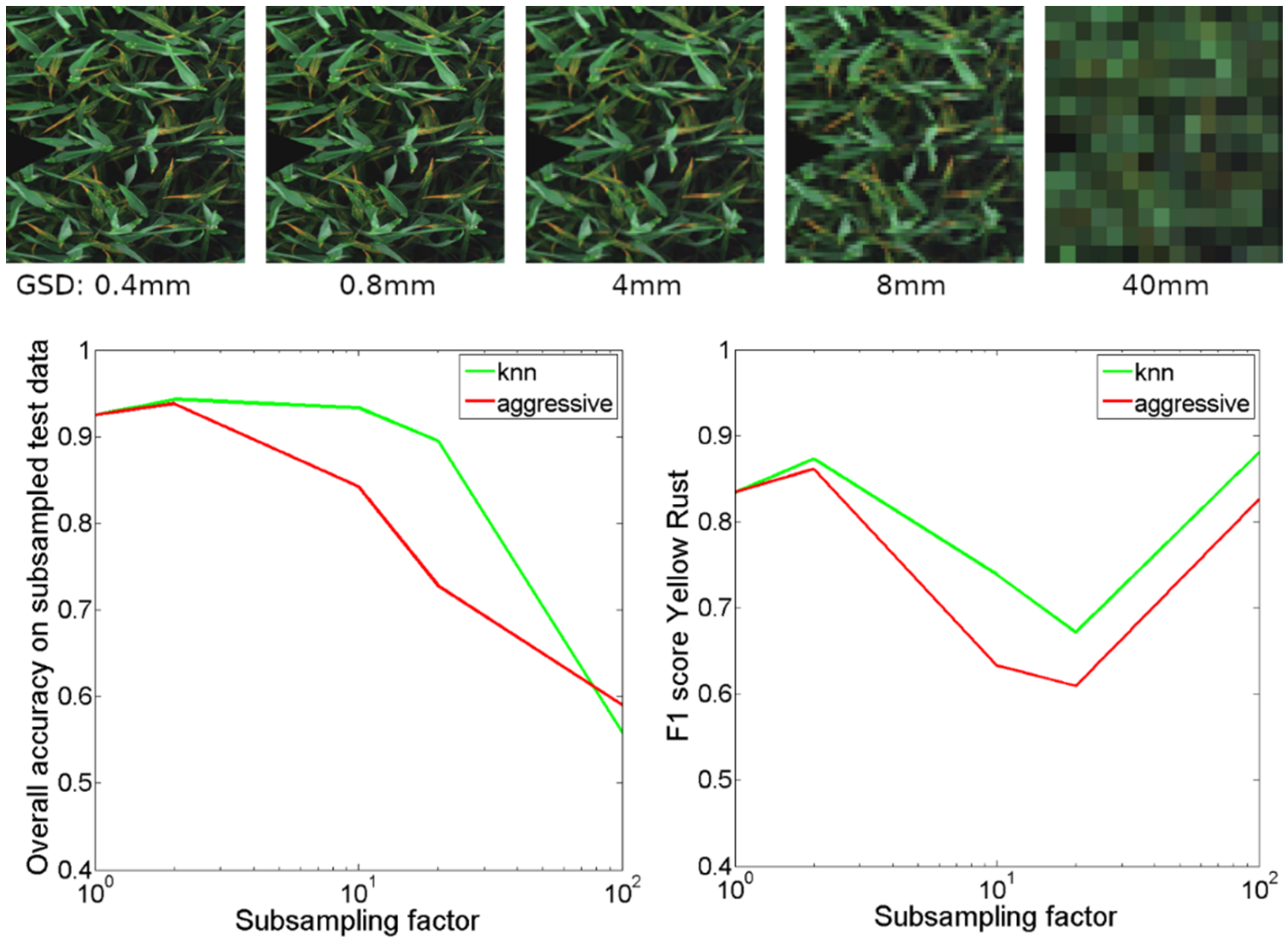
The un-sampled data had a GSD of approximately 0.4 mm (for Specim as well as Rikola). The UAV observations (20 m flight height) had a GSD of approximately 8 mm (Figure 9).
This approach did not regard the adaptation of the model to the new classification scale. By retraining the prediction, the accuracy may be improved, as the smoothing here also affected the data characteristics. However, even then, the disease-specific information will vanish at a certain level. We omitted this evaluation as the performance measures of the retrained models were not comparable anymore as the number of training data declined drastically, e.g., to around 100 samples for YR at higher subsampling scales.
The investigations allowed the definition of a minimal sampling distance at which the mixed information no longer allowed the prediction of plant diseases. Without retraining the model, the accuracy decreased at subsampling factors of 10 and 20. A low subsampling of 2 seems to have had no negative effects. Presumably, the included smoothing removed border cases and outliers which are hard to classify correctly. At higher subsampling levels, more and more mixed pixels occurred where the aggressive label subsampling tended to extend the image regions assigned to a class. Subsequently, the effect was more severe here. The accuracy of more than 50% at the final state was related to the dominant background, which provided a significant majority of test data at the high subsampling levels. It was not related to the ability to predict the presence of YR. This was demonstrated by the F1 score, a measure to quantify the performance of a multi-class prediction model on class level.
In this performance measure, the quality also decreased at subsampling factor of 10. Surprisingly, the F1 score increased to nearly optimal numbers at a subsampling factor of 100. Discussing this fact, it has to be noted that at the highest subsampling factor, only 119 YR samples were included in the data set, which are all correctly classified. Maybe this was related to the accuracy on the UAV scale, where the majority of geometric effects were averaged out. This point remains to be evaluated in further investigations, but it seems that subsampling by a factor of 100 removed the leaf structure completely, whereas at a lower subsampling factor, the leaf structure was still apparent but more and more effects of mixture become present. Without any leaf structure, the classification problem is simplified to the presence of YR within this part or even within the image. At low level disease severities, this will cause major problems, but here, the test data has been selected to show clear disease symptoms.
3.4. Optimal Sensor System for Plant Disease Detection
Two sensor systems were evaluated, both showing strengths and weaknesses. In direct comparison, the flying sensor system had strong advantages in usability, throughput, and commercial viability. The ground sensing system was much more sensitive, as a single symptom with a diameter of a few mm could be recorded. Such a spatial resolution could only be obtained by the flying system at a flight altitude of around 1 m above the canopy. However, with the used system this was not possible, as the downstream from the rotors would have strongly moved the canopy. Alternatively, an optical zoom could be applied, presumably reducing the light flux as well as the throughput of the overall system. This could be compensated for by an increased spatial resolution of the sensing array.
Summarizing, based on the experiments conducted during the presented study, we propose a focus on a UAV flying at low height in combination with a frame-based spectral camera sensing in around 15 equally distributed bands. A tunable band configuration would be an alternative that could use bands optimized for every single disease scenario, e.g., crop species, crop developmental stage, assumed disease setting, assumed symptom maturity. The spatial resolution should be set at around 1 mm GSD, a value that allows the detection small symptoms but neglects the high-frequency noise caused by the complex surface structure of plants [29,51].
4. Conclusions
This study investigated the detection of plant diseases using hyperspectral cameras at ground and UAV scales. In this context, the appropriate data analysis was decisively able to reach suitable results. Supervised classification has the advantage of separating disease-related signals from a huge amount of natural biological, geometrical, and sensor-related variability within a hyperspectral image of a crop canopy in the field. We proved that hyperspectral imaging in combination with supervised classification and regression showed good accordance to visual assessment at the ground. This allows questions to be addressed regarding the transfer of information between different scales and sensors. We showed that a feature selection was able to increase the prediction accuracy if it was performed on the analyzed data set. In contrast, scale or sensor transfer of selected feature sets was not successful, and was even less predictive than an uninformed regularly sampled feature set. This highlighted the importance of a precise specification of a prediction task by representative data samples. Deviations in data characteristics can significantly impair the performance of a data analysis pipeline or a tailored sensor in real-life applications.
This study sets a basis for ongoing research. New, upcoming sensors fulfilling the demands defined in this study might also cope with the current disadvantages. Consequently, there is a high probability that the defined flying sensor system with high resolution spectral camera, computing capabilities, and self-localization will be realized. Adapted legal conditions would allow an integrated system of field managing software, remote sensing based predictions, and current observations from the field using an automatized UAV.
Author Contributions
Conceptualization, D.B., J.B. and A.-K.M.; methodology, D.B. and J.B.; software, D.B. and J.B.; validation, D.B. and J.B.; formal analysis, D.B. and J.B.; investigation, D.B., J.B. and A.-K.M.; resources, D.B., J.B. and A.-K.M.; data curation, D.B., J.B. and A.-K.M.; writing—original draft preparation, D.B. and J.B.; writing—review and editing, D.B., J.B. and A.-K.M.; visualization, D.B., J.B. and A.-K.M.; supervision, J.B. and A.-K.M.; project administration, A.-K.M.; funding acquisition, A.-K.M.
Funding
This work was funded by BASF Digital Farming.
Acknowledgments
The authors would like to thank Onno Muller (Research Center Jülich, Germany) for providing the basic Phytobike frame, Thorsten Kraska for general support at Campus Klein-Altendorf and Winfried Bungert (Campus Klein-Altendorf, Germany) for implementation of cultivation measures during the vegetation period.
Conflicts of Interest
The authors declare no conflict of interest.
References
- West, J.; Bravo, C.; Oberti, R.; Lemaire, D.; Moshou, D.; McCartney, A. The potential of optical canopy measurement for targeted control of field crop diseases. Ann. Rev. Phytopathol. 2003, 41, 593–614. [Google Scholar] [CrossRef] [PubMed]
- Hillnhütter, C.; Mahlein, A.K.; Sikora, R.A.; Oerke, E.C. Remote sensing to detect plant stress induced by Heterodera schachtii and Rhizoctonia solani in sugar beet fields. Field Crops Res. 2011, 122, 70–77. [Google Scholar] [CrossRef]
- Bravo, C.; Moshou, D.; West, J.; McCartney, A.; Ramon, H. Early disease detection in wheat fields using spectral reflectance. Biosyst. Eng. 2003, 84, 137–145. [Google Scholar] [CrossRef]
- Mewes, T.; Franke, J.; Menz, G. Spectral requirements on airborne hyperspectral remote sensing data for wheat disease detection. Precis. Agric. 2011, 12, 795–812. [Google Scholar] [CrossRef]
- Mirik, M.; Jones, D.C.; Price, J.A.; Workneh, F.; Ansley, R.J.; Rush, C.M. Satellite remote sensing of wheat infected by wheat streak mosaic virus. Plant Dis. 2011, 95, 4–12. [Google Scholar] [CrossRef]
- Gebbers, R.; Adamchuk, V.I. Precision agriculture and food security. Science 2010, 327, 828–831. [Google Scholar] [CrossRef]
- Mahlein, A.K.; Kuska, M.T.; Behmann, J.; Polder, G.; Walter, A. Hyperspectral sensors and imaging technologies in phytopathology: State of the art. Ann. Rev. Phytopathol. 2018, 56, 535–558. [Google Scholar] [CrossRef]
- Wahabzada, M.; Mahlein, A.K.; Bauckhage, C.; Steiner, U.; Oerke, E.C.; Kersting, K. Plant phenotyping using probabilistic topic models: Uncovering the hyperspectral language of plants. Sci. Rep. 2016, 6, 22482. [Google Scholar] [CrossRef]
- Whetton, R.; Hassall, K.; Waine, T.W.; Mouazen, A. Hyperspectral measurements of yellow rust and fusarium head blight in cereal crops: Part 1: Laboratory study. Biosyst. Eng. 2017, 166, 101–115. [Google Scholar] [CrossRef]
- Whetton, R.; Waine, T.; Mouazen, A. Hyperspectral measurements of yellow rust and fusarium head blight in cereal crops: Part 2: On-line field measurement. Biosyst. Eng. 2018, 167, 144–158. [Google Scholar] [CrossRef] [Green Version]
- Mahlein, A.K. Plant disease detection by imaging sensors—Parallels and scientific demands for precision agriculture and plant phenotyping. Plant Dis. 2016, 100, 241–251. [Google Scholar] [CrossRef] [PubMed]
- Thomas, S.; Kuska, M.T.; Bohnenkamp, D.; Brugger, A.; Alisaac, E.; Wahabzada, M.; Behmann, J.; Mahlein, A.K. Benefits of hyperspectral imaging for plant disease detection and plant protection: A technical perspective. J. Plant Dis. Prot. 2018, 125, 5–20. [Google Scholar] [CrossRef]
- Bravo, C.; Moshou, D.; Oberti, R.; West, J.; McCartney, A.; Bodria, L.; Ramon, H. Foliar disease detection in the field using optical sensor fusion. Agric. Eng. Int. 2004, 6. [Google Scholar]
- Franke, J.; Menz, G. Multi-temporal wheat disease detection by multi-spectral remote sensing. Precis. Agric. 2007, 8, 161–172. [Google Scholar] [CrossRef]
- Huang, W.; Lamb, D.W.; Niu, Z.; Zhang, Y.; Liu, L.; Wang, J. Identification of yellow rust in wheat using in-situ spectral reflectance measurements and airborne hyperspectral imaging. Precis. Agric. 2007, 8, 187–197. [Google Scholar] [CrossRef]
- Lan, Y.B.; Chen, S.D.; Fritz, B.K. Current status and future trends of precision agricultural aviation technologies. Int. J. Agric. Biol. Eng. 2017, 10, 1–17. [Google Scholar]
- Devadas, R.; Lamb, D.W.; Simpfendorfer, S.; Backhouse, D. Evaluating ten spectral vegetation indices for indentifying rust infection in individual wheat leaves. Precis. Agric. 2009, 10, 459–470. [Google Scholar] [CrossRef]
- Ashourloo, D.; Mobasheri, M.R.; Huete, A. Developing two spectral indices for detection of wheat leaf rust (Puccinia triticina). Remote Sens. 2014, 6, 4723–4740. [Google Scholar] [CrossRef]
- Cao, X.; Luo, Y.; Zhou, Y.; Fan, J.; Xu, X.; West, J.S.; Duan, X.; Cheng, D. Detection of powdery mildew in two winter wheat plant densities and prediction of grain yield using canopy hyperspectral reflectance. PLoS ONE 2015, 10. [Google Scholar] [CrossRef]
- Blackburn, G.A. Hyperspectral remote sensing of plant pigments. J. Exp. Bot. 2007, 58, 855–867. [Google Scholar] [CrossRef]
- Gitelson, A.A.; Keydan, G.P.; Merzlyak, M.N. Three-band model for noninvasive estimation of chlorophyll, carotenoids, and anthocyanin contents in higher plant leaves. Geophys. Res. Lett. 2006, 33, L11402. [Google Scholar] [CrossRef]
- Roosjen, P.P.J.; Suomalainen, J.M.; Bartholomeus, H.M.; Clevers, J.G.P.W. Hyperspectral reflectance anisotropy measurements using a pushbroom spectrometer on an unmanned aerial vehicle—Results for barley, winter wheat and potato. Remote Sens. 2016, 8, 909. [Google Scholar] [CrossRef]
- Moshou, D.; Bravo, C.; West, J.; Wahlen, T.; McCartney, A.; Ramon, H. Automatic detection of ‘yellow rust’ in wheat using reflectance measurements and neural networks. Comput. Electron. Agric. 2004, 44, 173–188. [Google Scholar] [CrossRef]
- Zhang, J.; Pu, R.; Huang, W.J.; Yuan, L.; Luo, J.; Wang, J. Using in-situ hyperspectral data for detecting and discriminating yellow rust disease from nutrient stresses. Field Crop Res. 2012, 134, 165–174. [Google Scholar] [CrossRef]
- Zheng, Q.; Huang, W.; Cui, X.; Dong, Y.; Shi, Y.; Ma, H.; Liu, L. Identification of wheat yellow rust using optimal three-band spectral indices in different growth stages. Sensors 2019, 19, 35. [Google Scholar] [CrossRef]
- Azadbakht, M.; Ashourloo, D.; Aghighi, H.; Radiom, S.; Alimohammadi, A. Wheat leaf rust detection at canopy scale under different LAI levels using machine learning techniques. Comput. Electron. Agric. 2019, 156, 119–128. [Google Scholar] [CrossRef]
- Chen, W.; Wellings, C.; Chen, X.; Kang, Z.; Liu, T. Wheat stripe (yellow) rust caused by Puccinia striiformis f. sp. tritici. Mol. Plant. Pathol. 2014, 15, 433–446. [Google Scholar] [CrossRef]
- Yu, K.; Anderegg, J.; Mikaberidze, A.; Petteri, K.; Mascher, F.; McDonald, B.A.; Walter, A.; Hund, A. Hyperspectral canopy sensing of wheat Septoria tritici blotch disease. Front. Plant Sci. 2018, 9, 1195. [Google Scholar] [CrossRef]
- Behmann, J.; Mahlein, A.K.; Rumpf, T.; Romer, C.; Plümer, L. A review of advanced machine learning methods for the detection of biotic stress in precision crop protection. Precis. Agric. 2015, 16, 239–260. [Google Scholar] [CrossRef]
- Camps-Valls, G.; Tuia, D.; Bruzzone, L.; Benediktsson, J.A. Advances in hyperspectral image classification: Earth monitoring with statistical learning methods. IEEE Signal Process. Mag. 2014, 31, 45–54. [Google Scholar] [CrossRef]
- Lowe, A.; Harrison, N.; French, A.P. Hyperspectral image analysis techniques for the detection and classification of the early onset of plant disease and stress. Plant Methods 2017, 13, 80. [Google Scholar] [CrossRef] [PubMed]
- Singh, A.; Ganapathysubramanian, B.; Singh, A.K.; Sarkar, S. Machine learning for high-throughput stress phenotyping in plants. Trends Plant Sci. 2016, 21, 110–124. [Google Scholar] [CrossRef] [PubMed]
- Barnes, R.J.; Dhanoa, M.S.; Lister, S.J. Standard normal variate transformation and de-trending of near-infrared diffuse reflectance spectra. Appl. Spectrosc. 1989, 43, 772–777. [Google Scholar] [CrossRef]
- Kruse, F.A.; Lefkoff, A.B.; Boardman, J.W.; Heidebrecht, K.B.; Shapiro, A.T.; Barloon, P.J.; Goetz, A.F.H. The spectral image processing system (SIPS)—Interactive visualization and analysis of imaging spectrometer data. Remote Sens. Environ. 1993, 44, 145–163. [Google Scholar] [CrossRef]
- Cortes, C.; Vapnik, V. Support-Vector networks. Mach. Learn. 1995, 20, 273–297. [Google Scholar] [CrossRef]
- Chang, C.C.; Lin, C.J. LIBSVM: A library for support vector machines. ACM Trans. Intell. Syst. Technol. 2011, 2, 27. [Google Scholar] [CrossRef]
- Behmann, J.; Steinrücken, J.; Plümer, L. Detection of early plant stress responses in hyperspectral images. ISPRS 2014, 93, 98–111. [Google Scholar] [CrossRef]
- Guyon, I.; Elisseeff, A. An introduction to variable and feature selection. J. Mach. Learn. Res. 2003, 3, 1157–1182. [Google Scholar]
- Parker, S.R.; Shaw, M.W.; Royle, D.J. The reliability of visual estimates of disease severity on cereal leaves. Plant Pathol. 1995, 44, 856–864. [Google Scholar] [CrossRef]
- Nutter, F.W.; Gleason, M.L.; Jenco, J.H.; Christians, N.C. Assessing the accuracy, intra-rater repeatability, and inter-rater reliability of disease assessment systems. Phytopathology 1993, 83, 806–812. [Google Scholar] [CrossRef]
- Mahlein, A.K.; Rumpf, T.; Welke, P.; Dehne, H.W.; Plümer, L.; Steiner, U.; Oerke, E.C. Development of spectral indices for detectiong and identifying plant diseases. Remote Sens. Environ. 2013, 128, 21–30. [Google Scholar] [CrossRef]
- Chen, T.; Zhang, J.; Chen, Y.; Wan, S.; Zhang, L. Detection of peanut leaf spots disease using canopy hyperspectral reflectance. Comput. Electron. Agric. 2019, 156, 677–683. [Google Scholar] [CrossRef]
- Gates, D.M.; Keegan, H.J.; Schelter, J.C.; Weidner, V.R. Spectral properties of plants. Appl. Opt. 1965, 4, 11–20. [Google Scholar] [CrossRef]
- Curran, P.J. Remote sensing of foliar chemistry. Remote Sens. Environ. 1989, 30, 271–278. [Google Scholar] [CrossRef]
- Heim, R.H.J.; Jurgens, N.; Große-Stoltenberg, A.; Oldeland, J. ; The effect of epidermal structures on leaf spectral signatures of ice plants (Aizoaceae). Remote Sens. 2015, 7, 16901–16914. [Google Scholar] [CrossRef]
- Carter, G.A.; Knapp, A.K. Leaf optical properties in higher plants: Linking spectral characteristics to stress and chlorophyll concentrations. Am. J. Bot. 2001, 88, 677–684. [Google Scholar] [CrossRef]
- Pandey, P.; Ge, Y.; Stoerger, V.; Schnable, J.C. High throughput in vivo analysis of plant leaf chemical properties using hyperspectral imaging. Front. Plant Sci. 2017, 8, 1348. [Google Scholar] [CrossRef]
- Gay, A.; Thomas, H.; James, C.; Taylor, J.; Rowland, J.; Ougham, H. Nondestructive analysis of senescence in mesophyll cells by spectral resolution of protein synthesis-dependent pigment metabolism. New Phytol. 2008, 179, 663–674. [Google Scholar] [CrossRef]
- Bohnenkamp, D.; Kuska, M.T.; Mahlein, A.K.; Behmann, J. Hyperspectral signal decomposition and symptom detection of wheat rust disease at the leaf scale using pure fungal spore spectra as reference. Plant Pathol. 2019, 68, 1188–1195. [Google Scholar] [CrossRef]
- Elvidge, C.D. Visible and near infrared reflectance characteristics of dry plant materials. Int. J. Remote Sens. 1990, 11, 1775–1795. [Google Scholar] [CrossRef]
- Kuska, M.; Wahabzada, M.; Leucker, M.; Dehne, H.W.; Kersting, K.; Oerke, E.C.; Steiner, U.; Mahlein, A.K. Hyperspectral phenotyping on the microscopic scale: Towards automated characterization of plant-pathogen interactions. Plant Methods 2015, 11, 28. [Google Scholar] [CrossRef] [PubMed]
Figure 1.
Field trial layout (RGB stitch from unmanned aerial vehicle (UAV) images) at the research station Campus Klein-Altendorf (Rheinbach, Germany) of winter wheat varieties Bussard and Asano in 2018, with treatment declaration and measurement strategy. The trial was designed in two long rows of plots to reduce the number of turns and keep continuous measurements.

Figure 2.
Schematic overview of the course of the 2018 vegetation period. For each calendar week, the actions are presented and disease occurrence of yellow rust (YR) is shown. Weekly assessments and measurements were performed during the vegetation period (CW = calendar week; BBCH = growing stage).

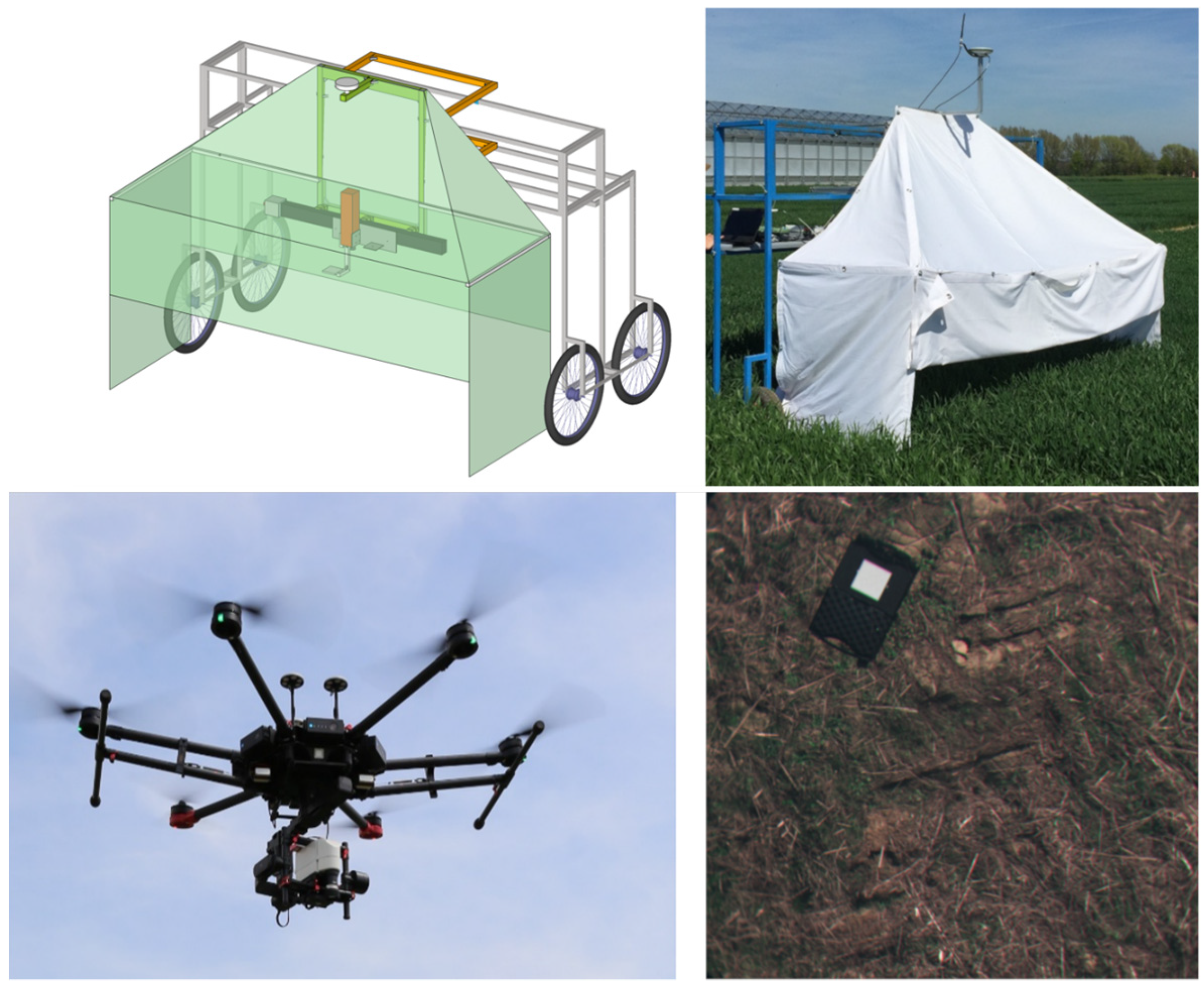
Figure 3.
Construction plan of the Phytobike (top left) and the final appearance in the field including the cotton diffuser (top right). The UAV system used, consisting of a DJI Matrice 600 and a Rikola hyperspectral camera (bottom left). Normalization was performed using a 50% grey reference panel (bottom right).

Figure 4.
Underlying workflow of data assessment to compare different prediction algorithms and evaluate the value of information about selected features at different scales. SVM = support vector machine, SAM = spectral angle mapper.
Figure 4.
Underlying workflow of data assessment to compare different prediction algorithms and evaluate the value of information about selected features at different scales. SVM = support vector machine, SAM = spectral angle mapper.

Figure 5.
Visual comparison of the representative spectral angle mapper (SAM) classification (top left) and the support vector machine standard normal variate (SVM SNV) classification (top right) with the original RGB visualization of the corresponding ground-based image of one representative measurement location of a plot inoculated with YR (bottom left). The image is captured with the hyperspectral camera Specim V10. The classes (bottom right) were generated from manual annotation of train and test data.

Figure 6.
Scatter plot of the relation between visual assessment and predicted disease ratios for yellow rust on 23 May 2018 before (left) and after the application of a linear calibration model (right). The calibration model had the purpose of compensating for scale differences in the prediction values.

Figure 7.
Prediction results of a YR infestation obtained by applying a leave-one-out procedure to the support vector regression (SVR) on the UAV scale. Each point represents a plot observation, and its color, the observation date (DD-MM).
Figure 7.
Prediction results of a YR infestation obtained by applying a leave-one-out procedure to the support vector regression (SVR) on the UAV scale. Each point represents a plot observation, and its color, the observation date (DD-MM).

Figure 8.
Results of the feature selection for the relevant wavebands for the classification of YR in the field on the ground (top) and UAV (bottom) scales. The accuracy reached for the different numbers of features (left) and the ranking of the inclusion within the feature subset (right) is displayed. RMSE = root mean square error.

Figure 9.
Visualization of spatial subsampling effects for the four investigated subsampling levels (images) and the effect of scale on accuracy and F1 score for the two different approaches knn (nearest neighbor) and an aggressive for subsampling the annotation.
Figure 9.
Visualization of spatial subsampling effects for the four investigated subsampling levels (images) and the effect of scale on accuracy and F1 score for the two different approaches knn (nearest neighbor) and an aggressive for subsampling the annotation.


Table 1.
Comparison of evaluation parameters obtained on test data for different data representations and prediction algorithms on the ground scale for the support vector machine (SVM) and the spectral angle mapper (SAM).
Table 1.
Comparison of evaluation parameters obtained on test data for different data representations and prediction algorithms on the ground scale for the support vector machine (SVM) and the spectral angle mapper (SAM).
| SVM Raw | SVM SNV | SVM Indices | SAM | |
|---|---|---|---|---|
| Accuracy | 91.9% | 92.9% | 90.2% | 81.4% |
| F1 disease score | 83.2% | 84.0% | 76.4% | 48.3% |
Table 2.
Performance values for different SVM and SVR models predicting the treatments of the wheat field experiment based on UAV observations.
Table 2.
Performance values for different SVM and SVR models predicting the treatments of the wheat field experiment based on UAV observations.
| Trait/Treatment | Performance |
|---|---|
| Fertilizer level | Accuracy = 82.3% |
| Fungicide | Accuracy = 91.5% |
| Fungicide + fertilizer level (four classes) | Accuracy = 71.4% |
| Disease detection (severity > 0) | Accuracy = 90.0% |
| Disease severity estimation | Correlation = 70.6% |
Table 3.
The six most important bands for selected plot traits at the UAV scale and ranking of the wavebands (in nm) for the importance of feature selection, beginning with the highest. Selected traits: fertilizer (Fert), fungicide (Fung), fungicide + fertilizer (Fert+Fung), yellow rust (YR) detection, yellow rust regression.
| Ranking | Fert | Fung | Fert + Fung | YR Detection | YR Regression |
|---|---|---|---|---|---|
| 1 | 767 | 727 | 734 | 797 | 832 |
| 2 | 725 | 804 | 887 | 881 | 510 |
| 3 | 648 | 762 | 545 | 601 | 867 |
| 4 | 557 | 648 | 559 | 706 | 874 |
| 5 | 627 | 594 | 517 | 874 | 587 |
| 6 | 704 | 767 | 748 | 594 | 594 |
Table 4.
Performance of the different feature sets for the YR detection based on ground observations.
Table 4.
Performance of the different feature sets for the YR detection based on ground observations.
| Ground Class. | All | UAV Select | Field Select | Equidistant | VI |
|---|---|---|---|---|---|
| # feature | 210 | 10 | 10 | 10 | 16 |
| Acc. | 92.9% | 87.4% | 88.9% | 89.2% | 90.2% |
| F1 disease | 0.84 | 0.694 | 0.751 | 0.732 | 0.764 |
Table 5.
Performance of the different feature sets for the YR regression based on UAV observations.
| UAV Regression | All | UAV Select | Field Select | Equidistant |
|---|---|---|---|---|
| # feature | 55 | 10 | 10 | 10 |
| R² | 0.63 | 0.69 | 0.57 | 0.61 |
| Corr. | 79.4% | 83.0% | 75.5% | 78.1% |
© 2019 by the authors. Licensee MDPI, Basel, Switzerland. This article is an open access article distributed under the terms and conditions of the Creative Commons Attribution (CC BY) license (http://creativecommons.org/licenses/by/4.0/).
Share and Cite
MDPI and ACS Style
Bohnenkamp, D.; Behmann, J.; Mahlein, A.-K. In-Field Detection of Yellow Rust in Wheat on the Ground Canopy and UAV Scale. Remote Sens. 2019, 11, 2495. https://0-doi-org.brum.beds.ac.uk/10.3390/rs11212495
AMA Style
Bohnenkamp D, Behmann J, Mahlein A-K. In-Field Detection of Yellow Rust in Wheat on the Ground Canopy and UAV Scale. Remote Sensing. 2019; 11(21):2495. https://0-doi-org.brum.beds.ac.uk/10.3390/rs11212495
Chicago/Turabian StyleBohnenkamp, David, Jan Behmann, and Anne-Katrin Mahlein. 2019. "In-Field Detection of Yellow Rust in Wheat on the Ground Canopy and UAV Scale" Remote Sensing 11, no. 21: 2495. https://0-doi-org.brum.beds.ac.uk/10.3390/rs11212495
Note that from the first issue of 2016, this journal uses article numbers instead of page numbers. See further details here.