Article

Spatial–Temporal Analysis of Land Cover Change at the Bento Rodrigues Dam Disaster Area Using Machine Learning Techniques

Department of Geography and Geospatial Sciences, Kansas State University, Manhattan, KS 66506, USA
*
Author to whom correspondence should be addressed.
Remote Sens. 2019, 11(21), 2548; https://0-doi-org.brum.beds.ac.uk/10.3390/rs11212548
Submission received: 13 September 2019 / Revised: 18 October 2019 / Accepted: 26 October 2019 / Published: 30 October 2019

Abstract

:
Disasters are an unpredictable way to change land use and land cover. Improving the accuracy of mapping a disaster area at different time is an essential step to analyze the relationship between human activity and environment. The goals of this study were to test the performance of different processing procedures and examine the effect of adding normalized difference vegetation index (NDVI) as an additional classification feature for mapping land cover changes due to a disaster. Using Landsat ETM+ and OLI images of the Bento Rodrigues mine tailing disaster area, we created two datasets, one with six bands, and the other one with six bands plus the NDVI. We used support vector machine (SVM) and decision tree (DT) algorithms to build classifier models and validated models performance using 10-fold cross-validation, resulting in accuracies higher than 90%. The processed results indicated that the accuracy could reach or exceed 80%, and the support vector machine had a better performance than the decision tree. We also calculated each land cover type’s sensitivity (true positive rate) and found that Agriculture, Forest and Mine sites had higher values but Bareland and Water had lower values. Then, we visualized land cover maps in 2000 and 2017 and found out the Mine sites areas have been expanded about twice of the size, but Forest decreased 12.43%. Our findings showed that it is feasible to create a training data pool and use machine learning algorithms to classify a different year’s Landsat products and NDVI can improve the vegetation covered land classification. Furthermore, this approach can provide a venue to analyze land pattern change in a disaster area over time.

Graphical Abstract

1. Introduction

Disasters triggered by natural or human processes not only cause considerable loss of life and economic disruption, but also can change land use and land cover and affect the environment [1,2,3]. Over the ten years from 2008 to 2017, there have been around 3,751 large-scale natural disasters recorded, of which 84.20% resulted from weather [4]. With the intervention of human activities and climate change, the frequency of disaster rapidly increased and it has become one main drivers for land use and land cover change at the local scale [5]. Land cover changes in a disaster area can include both temporary and long-time land cover change. Studying land pattern change in the disaster area is necessary because the disaster areas are typically located near agriculture or residence area, and disaster is the consequence of the interaction between human activity and environment. Either way can make remote sensing data became the primary dataset because of its convenience, efficiency, and consistency observation [6,7,8,9].
Remote sensing images can be used to analyze the damage of disaster by comparing the images of before and after the event, however, this initial step just provides some limited information. To fully understand the disaster area, we need to process remote sensing images to get more detailed information. For example, remote sensing images can be used to classify land use and land cover in disaster areas and analyze its pattern of change, or combining them with some social–economic factors to analyze the relationship between human activity and environment [10,11]. Nevertheless, there are some uncertainties about processing remote sensing images in disaster areas. For instance, different classification methods such as unsupervised and supervised classification could have different performance; feature selection can also affect final classification result because of the overfitting or underfitting problem; and the lack of sufficiently large amount of training samples could also affect final results [12,13,14,15]. In addition, because different year’s remote sensing images use different data collection methods, even if we chose the same interested areas, the process results could have some difference.
Some researchers have tried to use NDVI to classify agricultural areas and the accuracy of their results that are higher than 85% [16,17,18]. Compared with pixel-based classification, some scholars have also tried object-based image analysis (OBIA), and they concluded that this type of method can achieve higher performance than pixel-based classification [16,19,20,21]. With the advance of computational efficiency, machine learning methods have been increasingly used and shown to be powerful in a wide variety of scientific disciplines [22]. The remote sensing community has used machine learning based methods for nearly 20 years, and there are a large number of algorithms that can generate thematic maps [7,23,24]. One example of a machine learning method widely used in image classification is the support vector machine (SVM) developed in the early 1990s, but broadly used in the remote sensing community for the past 20 years [9,18,25]. For instance, many studies have used this algorithm to solve landslide susceptibility mapping, soil moisture estimation, and land use and land cover classification problems [9,20,26,27,28]. The core of its mechanism is to use a basis function to translate training data into a higher dimensional feature space, and find the optimal hyperplanes that separate classes with minimum classification errors [25]. The SVM is a supervised non-parametric kernel-based learning system rooted in the statistical learning theory. It is possible to achieve higher accuracy just using a smaller training data and minimizing classification error on unseen data without prior assumptions made on the probability distribution of the data.
Another commonly used machine learning algorithm is the decision tree (DT), which is a hierarchical model using rules to split independent variables into homogeneous decision regions [29]. Decision trees had also been broadly used in land use and land cover sciences to solve classification problems [7,13,25,30]. The basic idea of the decision tree is to use algorithms to select the input feature and threshold value at each splitting, and each node in a decision tree represents a feature in an instance to be classified, and each branch represents a value that the node can assume [23]. Because univariate decision trees have the ability to handle non-linear relationships between features and classes and process data measured on different scales, it can break a very complex classification problem into multiple stages of simpler decision-making processes [25,31,32,33].
An increasing number of studies have used these two machine learning algorithms to classify remote sensing images, but fewer of them applied these two algorithms and Landsat images to improve disaster area remote sensing image processing. We assumed that adding an additional feature like NDVI could improve image processing accuracy. In addition, most studies just extracted training data from processing images and used it to classify the same image. Though it is the main remote sensing image process method, this approach can cause some potential errors because of the quality of training data, especially considering the temporal scale. However, based on the flexibility of the machine learning algorithms, we can create a training pool to do classification, which could improve the accuracy of results and avoid some potential errors. Based on this analysis, we also hypothesized that is it possible to create a training data pool to classify different year’s images using these two algorithms.
These two machine learning algorithms have broadly been used in the remote sensing community to process images, but little is known about the performance of classifying different year’s remote sensing images. The goals of this study are three fold, (1) we tested how NDVI can improve the remote sensing images classification at disaster area; (2) we created a training pool and applied these two machine learning algorithms to classify different year’s remote sensing image and evaluated is performance; (3) we estimated land cover changes in this disaster area from 2000 to 2017 using processed results. To address this knowledge gap, we took as an example of the Bento Rodrigues tailing dam area, which collapsed on 5 November 2015, and has been described as the worst environmental disaster in Brazil’s history [34].

2. Study Area

We conducted our study at Bento Rodrigues dam disaster area located west of the municipality of Marianna, Minas Gerais state (Brazil), the latitudes and the longitudes are −20.23° and −43.42° (Figure 1). The broken tailing dam released about 55–62 million m3 of red mud into the Doce river and destroyed more than 900 hectares of agricultural area [35,36]. The study area includes the cities of Mariana, Ouro Preto, and Pte. Nova; and the river of Gualaxo do Norte, Gualaxo Do Sul, Carmo and Piranga. The climate in this area is tropical savanna, with hot and humid wet season (October to March) and mild dry season (April to September). The annual temperature is between 9 to 35 °C and the average of annual precipitation is 1491.3 mm. Considering the terms of land use (human economic purpose or intent applied to these attributes) and land cover (biophysical attributes of the earth’s surface), we focused on land cover in the disaster area [37]. It is in the Atlantic rain forest biome and because of its suitable climatic condition and growing population, the dominant land cover is agricultural [38]. Near river areas, forest fragmentation is more severe and mapping this area is the essential step to understand its land pattern changes and the relationship between human activity and environment system.

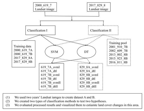
3. Materials and Methods

3.1. Data Collection and Pre-Processing

We collected path 217 and row 74 dry season Landsat 7 ETM+ and Landsat 8 OLI images from the USGS EROS Datacenter (http://eros.usgs.gov). The data we chose was in the same season (dry season) and less than 1% cloud cover (Table 1). After corrected the coordinate system and extracted study area, we calibrated raw images and converted digital numbers into the top of atmosphere radiation to minimize the atmosphere effect using FLAASH (Fast Line-of-slight Atmospheric Analysis of Spectral Hypercubes) module in ENVI 5.2 Software, which has been demonstrated that it works well in the atmospheric correction of multispectral image [39,40].
Using the acquired images, we created two datasets; dataset (A) contains six bands (blue, green, red, NIR, SWIR-1 and SWIR-2) reflectance information as features, and dataset (B), which added normalized difference vegetation index (NDVI) to those six bands. We used pixel-based image analysis to process image because satellite remote sensing-based pattern recognition can group population of pixels in broad classes as per their inherent characteristics (DN values) [17,41].
Finally, we used Google Map as a reference to determine six land cover classes (Water, Forest, Urban, Agriculture, Bareland, and Mine sites) based on the generally accepted land use and land cover classification system [42] (Table 2).

3.2. Training Data

Because the quality of training data plays a critical role in the machine learning based supervised classification, we used Google Map as a reference and randomly selected each land cover patterns in the whole study area. We had two procedures, first, we collected training data from 2000 and 2017 images and built classifier models to classify each year’s remote sensing images respectively. Second, to test the possibility of using the same training data to classify different year’s images, we created a training data pool, which is each land cover type’s training data from 2001, 2002, 2013, 2015 and 2016 remote sensing images. Then, these training data were used to build a classifier model to classify 2000 and 2017 images. It is emphasized that we chose dry season remote sensing images, and some agricultural area were at fallow condition. To avoid potential errors, we selected both crop-covered areas and fallow areas as our agriculture land cover training data.

3.3. Support Vector Machine and Decision Tree

When we use remote sensing images to process data, they typically contain thousands or even millions of pixels. Even if we can select training data, the selected data are too small to apply to the whole image. Previous studies have proved that SVM is a reliable approach to handle high-dimensional data with a limited training set and can achieve substantially higher classification accuracy [18,25,43].
In this study, we used an existing SVM algorithm to build classifier models [25,30]. Because the SVM is a kernel-based machine learning algorithm, comparing several kernel functions, we chose the radial basis function (RBF) kernel, which uses two parameters, contains penalty (C) and kernel width (γ) and it is commonly used in the literature for the classification of remote sensing images [9,30,33,44]. To build optimal models, we chose the grid search method followed by [30] to find the best penalty and kernel width for the model. Once we determined the best parameters, the models were applied to the whole image, yielding the result.
Meanwhile, the second machine learning algorithm chosen in this study is the decision tree (DT), which is a hierarchical model composed of decision rules that recursively split independent variables into homogeneous zones and is also a commonly used machine learning approach in remote sensing community. Unlike support vector machine, which uses all available features simultaneously and makes a single membership decision for each pixel, DT uses a multi-stage or sequential approach to split chain of simple decision based on the results of sequential tests rather than a single and complex decision [33]. There are many existing algorithms for constructing decision tree models such as the Chi-square automatic interaction detector decision tree (CHAID), CART, C4.5 and J48 [24,33]. Considering the influence of accuracy factors such as pruning, boosting methods used and decision thresholds, in this study, we used a J48 decision tree algorithm which uses entropy (measurement of disorder of data) and information gain (measurement of association between inputs and outputs) to make decisions [32]. To improve the tree’s generalization capacity and avoid overfitting, we pruned trees by reducing structural complexity.

3.4. Model Process and Validation

ENVI 5.2 Software and scikit-learn of Python library [45] were chosen to finish this study and we did two types of classification. Classification method I is to test NDVI can improve the remote sensing image classification or not, and we used two datasets with each machine learning algorithm to build models. The process was to classify 2000 and 2017 images with their own training data (first procedure in 3.2). Classification method II fitted our second goal and we just chose the better dataset based on the classification method I result to do classification. The process was to use the training data pool (second procedure in 3.2) to classify 2000 and 2017 images. Since there are different types of processed results, to easily identify them, we created a short name. For example, 619_7A_svmI means the image was acquired at 6/19/2000 and it is Landsat 7 EMT+ image, then A means we used dataset (A), svm is the support vector machine algorithm and I means classification method I (Table 3). In addition, the results in this study just had year of 2000 and 2017, and we did not add year information in the short name.
With two different datasets and two types of machine learning algorithms, we had ten models. We set penalty from 0.1 to 100 and Kernel width from 0.1 to 0.5 to search the optimal model parameters of SVM algorithm and depth of tree is 10 for DT algorithm and all models needed to evaluate the performance of the model before we applied them to the whole study area. A ten-fold cross-validation technique was chosen because of its mild computational cost [46]. We calculated the average accuracy of the ten folds of each model and all models had higher than 97% cross-validation accuracy (Table 4). Generally, we found that SVM training models were constructing more accurate models than DT training models.
Many studies in remote sensing have proved that using the SVM algorithm to process images can reach better performance than decision tree [24,33]. After we classified images using classification method I and dataset A, we selected 619_7A_svmI and 829_8A_svmI and sampled some random areas to compare with Mapbiomas product at the same area. It is the land use and land cover map product operated by the Greenhouse Gas Emissions Estimation System (SEEG) from the Climate Observatory, and it is broadly used to analyze the relationship between human activity and land use and land cover change (http://mapbiomas.org/pages/database/mapbiomas_collection). The other reason we chose this product to validate our result was that it is difficult to find the historical thematic map in the study area. Compared with its same year’s product at the same area, the accuracies of our 2000 and 2017 results were 78.35% and 80.12%. There were some uncertainties about the processed images and Mapbiomas products such as different land cover scheme and different classification method, however, classification of original remote sensing images was not our first obligation in this study. We decided to use 619_7A_svmI and 829_8A_svmI as reference maps to do the following analysis.
To evaluate each land cover type’s performance, we also calculated their sensitivities (true positive rate), which can measure the proportion of actual positives that are correctly identified, and it is commonly used to evaluate results [47,48].
s e n s i t i v i t y i = p i p j i + p i ,
where: i is the current type of land cover, p is the i th land cover pixels that are correctly classified. p j i is the other types of land cover total pixels that incorrectly classified into the i th type of land cover.

4. Results

In this study, we used 2000 and 2017 dry season single remote sensing images to test two hypotheses. First, we processed remote sensing images with dataset A and B with the classification method I to test how NDVI improves the processing accuracy or not. Second, we classified these two remote sensing images with classification method II and dataset B using the training pool. We used processed image against A_svmI and B_svmII to calculated accuracy and Kappa, which are commonly metrics to evaluate land use and land cover classification in remote sensing community [24,49]. The overall accuracy (higher than 75.06%) and Kappa (higher than 0.59) of processed images has been listed in the Table 5.

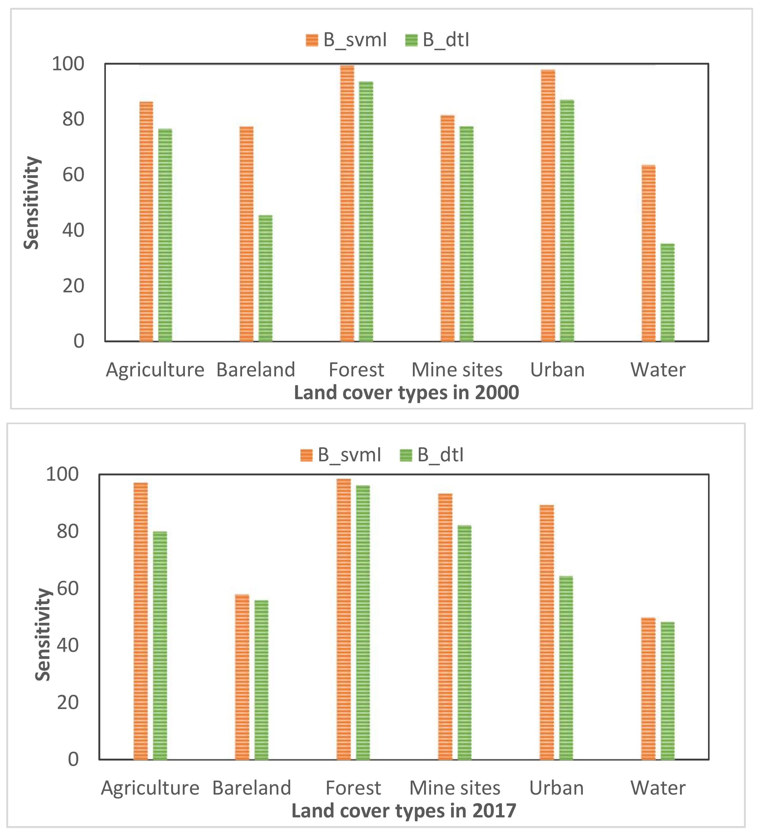
4.1. Performance of Processed Result with Adding NDVI as an Additional Feature

We did classification method I to test the performance of NDVI using dataset A and B. The results showed that accuracies of the 2000 classified images (with dataset B and two machine learning algorithms) were both higher than 80% but the Kappa value ranged from 0.69 to 0.86. The 2017 classified images (with dataset B and two machine learning algorithms) also gave us similar results, but the overall quality of processed images is better than the 2000 images according to accuracy and Kappa (Table 5). It was noticeable that SVM achieved a higher accuracy than DT in the 2000 and 2017 processed images, and some scholars also used support vector machines and cart algorithms with limited training data to classify land use and land cover map and got similar results [24].
The disaster area is covered by Forest and Agricultural land cover, and to deeply analyze each land cover performance with dataset B, we used Equation (1) to calculate each land cover type’s sensitivity using processed images against A_svmI images (Figure 2). The results showed that Agriculture and Forest land covers had higher sensitivities than Bareland, Urban and Water land covers. Particularly, Forest in the 2000 and 2017 images had the highest sensitivity, and a similar condition also happened in Agriculture land cover type. This finding determined that NDVI can improve the vegetated land cover types image processing.
Furthermore, our results also showed that the sensitivity of Bareland and Water land cover types had more variability using SVM and DT algorithms compared 2000 images and 2017 images. Though NDVI can just improve the performance of vegetated land cover, our result also indicated that Mine sites can have a decent performance in both 2000 and 2017 using dataset B.

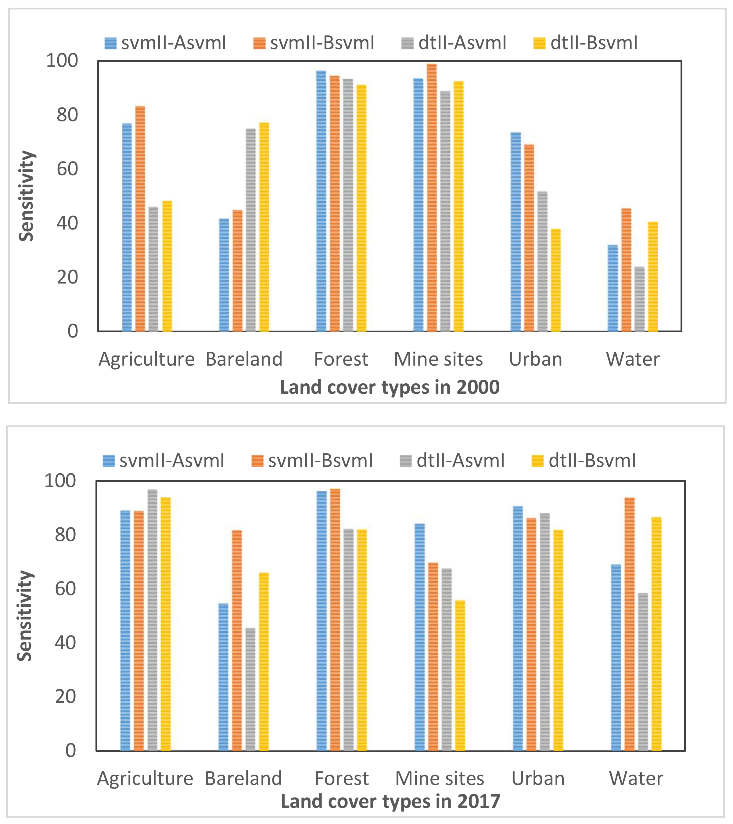
4.2. Performance Assessment of Classified Images using the Training Pool

One of our goals was to test a training data pool and use machine learning algorithms to classify different year’s Landsat images. Since dataset B had a better performance than dataset A with classification method I, we just chose dataset B to process the classification method II. The processed results showed that accuracies of 2000 and 2017 results were reasonable with the average accuracy of 82.93%. But 619_7B_svmII and 829_8B_svmII had higher accuracy (greater than 80%) and kappa values (greater than 0.7) than 619_7B_dtII and 829_8B_dtII results (Table 5).
Furthermore, we used processed images against classification I result (with dataset A and B using the SVM algorithm) to calculate each land cover type’s sensitivity using Equation (1) (Figure 3). Overall, the 2017 processed images had better performance than the year 2000 images with each land cover type. Comparing the processed results, it is notable that Forest and Mine sites in 2000 and Agriculture, Forest and Urban in 2017 had better performance either using the SVM algorithm or the DT algorithm.
In particular, each land cover type had different sensitivities with these two machine learning algorithms. For example, in the 2000 image, Agriculture and Urban had much higher sensitivities when using the SVM algorithm, but Bareland had higher sensitivity when applied the DT algorithm. In the 2017 image, Bareland, Mine sites and Water land covers had different sensitivities. In this study, these land cover types are more complex, and it is not easy to identify them using dry season images. Even if we created the same training pool to process the images, because of the different mechanisms of the algorithm, the performance was different.

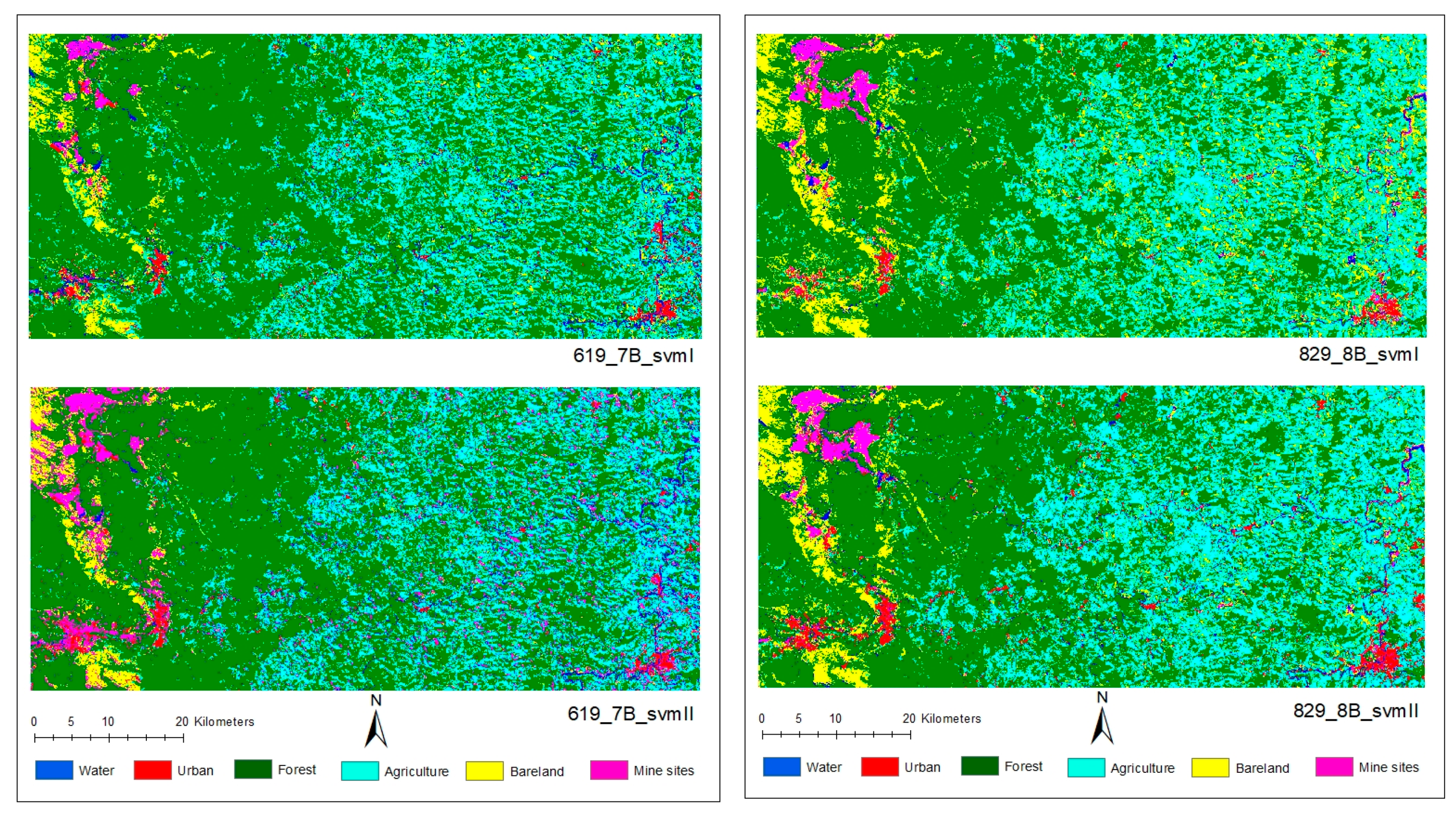
4.3. Land Cover Maps

The ultimate goal of processing remote sensing images is to generate a land cover map and analyze its pattern changes; after we discussed each land cover type’s sensitivity, we chose to visualize 2000 and 2017 land cover maps with dataset (B) using classification method I and II (Figure 4 and Figure 5). Overall, our results clearly identified main land cover types in this disaster area and maps that applied classification method II with the SVM algorithm had better performance.
Though main land cover types can be identified from the results, comparing classification I and II images using the SVM algorithm, we still found some interesting results. Generally, we can identify river channels and small cities from classification II images (Figure 4). Though 829_8B_svmII image can clearly identify some residue along the river channels, the Mine sites in 619_7B_svmII was much bigger than 619_7B_svmI, especially near Oumro Preto and Mariana cities.
The results that used the DT algorithm were less accurate than the results that used the SVM algorithm (Figure 5); 619_7B_dtI and 829_8B_dtI can both identify each land cover types and had a general performance, but there was a problem in 619_7B_dtII and 829_8B_dtII. The Bareland area in 619_7B_dtII was much larger than 619_7B_dtI.

4.4. Land Cover Change Estimation

We calculated each pixel’s land cover to estimate each land cover changes during these 17 years. In particular, we did three different calculations by removing much higher or lower pixel values of each land cover types (each land cover average pixels from classification method I and II, each land cover average pixels from classification method I, and each land cover pixels from classification method II with dataset B and the SVM algorithm) (Figure 6). During these 17 years, our results indicated that the Forest decreased by about 12.43%. The study area is located in the Atlantic forest biome, which consisted of evergreen and seasonally-dry forests, however, since the 16th century following the European arrival in Brazil, this area was deforested, in favor of urbanization and agricultural expansion, the forest has decreased to 10% of its original size. Our results showed that Agricultural and Bareland areas increased 19.22% and 37.75%. Near river valley areas, because of accessibility to water resources, people frequently converted forest to urban areas or agriculture areas and forest fragmentation is much worse than other areas [50]. Besides, the study area contains a big mining dam at the top left corner, and with these year’s development, its size increased 117.76%.

5. Discussion

5.1. General Analysis of the Processed Methods

The study area considered here was a good case study to estimate land cover changes over time, but interpretations of images are not easy because of having some limitations such as random noise, cloud cover, spatial resolution, and temporal resolution problems. In this study, we tried to test if NDVI can improve the results of image processing and use a training pool to classify different year’s remote sensing images. The overall accuracy of our classification I results are higher than 77.50% (Table 5) and each land cover’s sensitivity analysis indicated that that NDVI can modestly improve the performance of vegetated land cover types in the disaster area. Besides, our classification II results determined that creating a training pool to process different year’s remote sensing images is a feasible approach to analyze land use and land cover change in a disaster area at a local scale. However, according to our results, there are still some details that need to be discussed.
In classification method I, we used two datasets and two machine learning algorithms to classify 2000 and 2017 images, and the only difference with these two datasets is the NDVI feature. Some studies have shown that NDVI is a good indicator to detect and monitor vegetation condition, especially during vegetation growing season [14,18,51]. In addition, some researchers pointed out that vegetated land cover were found to have better NDVI agreement than non-vegetated land cover types using different platforms such as Landsat 8 OLI, Landsat 7 ETM+ and Moderate Resolution Imaging Spectroradiometer (MODIS) [52]. When we process remote sensing images that are in vegetation-covered areas such as grassland, cropland and forests, we can definitely improve the accuracy of the result [14,53], and our results also are in line with these studies. However, comparison of each land cover’s sensitivity with different machine learning algorithms and different years (Figure 2), we found that some land covers such as Bareland and Water in 2000 images have more unstable sensitivity. In the disaster area, these two land covers are more complex than other types land covers; even if we add one more feature (NDVI), these land covers still cause some errors. In addition, we also noticed that Bareland in 2017 image had lower sensitivity (50%) (Figure 2) and visualization results showed that the Bareland area is bigger than expected (Figure 4). We acquired remote sensing images at dry season, and some agricultural areas were at fallow season and this limitation is the main factor to affect the performance of Bareland. This finding also determined that classifying more complex land surface that contains Urban or Bareland land cover types, NDVI does not help to improve the performance.
In the classification method II, we used dataset B to create a training pool and classified 2000 and 2017 images with support vector machine and decision tree algorithms. Sensitivity analysis claimed that this image processing method has better performance than classification method I. To analyze land use and land cover change over time, there are some common methods such as image differencing, principal component analysis, and post-classification comparison [54]. The general idea of these methods is that we need to classify remote sensing images and compare the different processed images, which make the image classification become the most important part during the change detection analysis. Many studies have tried these two algorithms to classify single year’s remote sensing image and their classification results indicated that these two machine learning algorithms are the robust methods to process remote sensing images [17,20,21,25]. However, when considering different year’s remote sensing images, processing methods such as classification I in this study could run into some errors and increase the bias of processed image analysis. Compared with the classification I method, we found that classification II method has better performance than classification I method, which can reduce the potential errors and improve change detection analysis. For example, the overall quality of the processed images is better because we can identify more details in the disaster area (Figure 4 and Figure 5). Nevertheless, there are some uncertainties in some land covers such as Bareland, Water and Urban. We carefully selected training data from different year’s remote sensing images and optimized the classifier model, but the sensitivities of these three land covers are still low in 2000 images. In spite of these shortcomings, our findings still provided a new approach to analyze land use and land cover change detection at a local scale.

5.2. Limitations about Remote Sensing Images and Algorithms

We chose the Landsat 7 EMT+ and the Landsat 8 OLI images to do the classification, and results indicated that the Landsat 8 images had better performance than the Landsat 7 image. Compared with Landsat 7, Landsat 8 has higher 12-bit radiometric resolution and more precise geometry, which can avoid potential error and achieve a better performance. In addition, different types of sensors, spectral band responses, instrument performances, and atmospheric conditions at the time of observation could increase bias in each remote sensing image [52]. For example, near infrared band in Landsat 7 ETM+, the range is from 0.772 to 0.898 um, but in Landsat 8 OLI, the range changed to 0.851–0.879 um to avoid water vapor absorption. In addition, the OLI sensor in Landsat 8 employs the pushbroom technology, which enables the data acquisition with much better signal-to-noise (SNR) performance and higher radiometric resolution [55].
The limitation of the spatial resolution can also reduce the accuracy of remote sensing image processing. For example, many studies used Landsat product to process remote sensing images, because of its finer spatial resolution compared to MODIS or other coarser resolution data products. But it is highlighted that one single pixel in Landsat product is about 900 m2 and the one pixel could just have one type of land cover or could mix with others. In our study, one possible reason of some land cover types had lower sensitivity is mixed pixels, which could cause misclassification. For instance, some river channels are narrow in this disaster area and one pixel could have reflectance errors with mixed land cover. In addition, in this study, dry season remote sensing images could arise problems. For example, some agriculture areas were fallow during the dry season, and the boundary of mine areas had similar reflectance with some urban areas, even if we had Google Map as a reference, there could also occurred misclassification problems.
Recently, support vector machine and decision tree algorithms have been broadly used by the remote sensing community to solve classification problems, and some studies also concluded that support vector machine can generate better results compared to the decision tree algorithm [7,24,56]. Processing remote sensing images is a difficult task; our results showed that decision tree is not the best one to process different year’s remote sensing images using the classification II method.
With the development of computer sciences, some studies have started to apply deep learning technique to process remote sensing images [57,58,59]. Because of the unique character of remote sensing images, some deep learning techniques such as Convolutional Neural Network (CNN) and Recurrent Neural Network (RNN) have been proven to generate a higher performance [60,61,62]. Nevertheless, there are some parts that need to be improved in future research. First, we can use the same Landsat products and collect more data to avoid different Landsat product problems and solve dry season reflectance problems. Second, to improve the accuracy of the result, we can consider an object-based approach and add more secondary information as features to improve the accuracy.

6. Conclusions

Disasters are an unpredicted way to change land use and land cover and affect local environment; remote sensing images are primary data sources to map land cover and analyze land cover change. In this study, we used two datasets and two classification methods to test whether NDVI can improve the accuracy of processing images and if it is easy to create a training data pool to classify different years Landsat images use support vector machine and decision tree algorithms. We collected the dry season of 2000, 2001, 2002, 2013, 2015, 2016, and 2017 images and did atmosphere correction. After image preparation, we classified 2000 and 2017 Landsat images using classification methods I and II.
We validated training models using ten-fold cross-validation and chose optimal models to process the whole disaster area. We assessed classification I images, and the overall accuracy was higher than 80%. Analyzing each land cover’s sensitivities, we found that NDVI can help improve the accuracy of vegetated land cover types. After we got classification II images of 2000 and 2017, we also assessed their accuracies and calculated each land cover type’s sensitivity, and the overall accuracy was around 80%. Finally, we estimated each land cover change, and found that from 2000 to 2017, Forests decreased by 174.64 km2 but the Urban area, Agriculture and Mine sites increased by 13.69 km2, 121.34 km2 and 27.15 km2, respectively.
In the present study, although there are some limitations about remote sensing data and machine learning algorithms, we still conclude that it is feasible to use the same training data pool to classify different year’s Landsat images using support vector machine and decision tree algorithms. We also proved that NDVI as a broadly used vegetation index can improve the accuracy of classification at vegetated covered land in disaster areas. Our findings can apply to other similar areas with limited data sources to help land planners to effectively manage land use and land cover and analyze land changes over time.

Author Contributions

Conceptualization, D.G.G. and M.M.C.; Data curation, D.L.; Formal analysis, D.L.; Funding acquisition, D.G.G. and M.M.C.; Methodology, D.L. and D.G.G.; Resources, M.M.C.; Software, D.L.; Validation, D.L.; Visualization, D.L.; Writing–original draft, D.L.; Writing–review & editing, D.G.G. and M.M.C.

Funding

This research received no external funding, but D.L. received scholarship from the department of Geography and Geospatial Sciences and used it in this research. The APC was funded in part by the Kansas State University Open Access Publishing Fund.

Acknowledgments

We would like to thank the anonymous reviewers for their constructive comments in improving the manuscript. We also thank USGS for providing Landsat images with free of charge.

Conflicts of Interest

The authors declare no conflict of interest. The funders had no role in the design of the study; in the collection, analyses, or interpretation of data; in the writing of the manuscript, or in the decision to publish the results.

References

  1. Aires, U.R.V.; Santos, B.S.M.; Coelho, C.D.; Da Silva, D.D.; Calijuri, M.L. Changes in land use and land cover as a result of the failure of a mining tailings dam in Mariana, MG, Brazil. Land Use Policy 2018, 70, 63–70. [Google Scholar] [CrossRef]
  2. Kavzoglu, T.; Sahin, E.K.; Colkesen, I. Landslide susceptibility mapping using GIS-based multi-criteria decision analysis, support vector machines, and logistic regression. Landslides 2014, 11, 425–439. [Google Scholar] [CrossRef]
  3. Chen, W.; Chai, H.; Zhao, Z.; Wang, Q.; Hong, H. Landslide susceptibility mapping based on GIS and support vector machine models for the Qianyang County, China. Environ. Earth Sci. 2016, 75, 1–13. [Google Scholar] [CrossRef]
  4. IFRC. Leaving Millions Behind; IFRC: Geneva, Switzerland, 2018; ISBN 9782970128908. [Google Scholar]
  5. Habib, M.S.; Sarkar, B. An Integrated Location-Allocation Model for Temporary Disaster Debris Management under an Uncertain Environment. Sustainability 2017, 9, 716. [Google Scholar] [CrossRef]
  6. Rogan, J.; Chen, D. Remote sensing technology for mapping and monitoring land-cover and land-use change. Prog. Plan. 2004, 61, 301–325. [Google Scholar] [CrossRef]
  7. Otukei, J.; Blaschke, T. Land cover change assessment using decision trees, support vector machines and maximum likelihood classification algorithms. Int. J. Appl. Earth Obs. Geoinf. 2010, 12, S27–S31. [Google Scholar] [CrossRef]
  8. Yuan, Z.; Khakzad, N.; Khan, F.; Amyotte, P. Risk analysis of dust explosion scenarios using bayesian networks. Risk Anal. 2015, 35, 278–291. [Google Scholar] [CrossRef] [PubMed]
  9. Mountrakis, G.; Im, J.; Ogole, C. Support vector machines in remote sensing: A review. ISPRS J. Photogramm. Remote. Sens. 2011, 66, 247–259. [Google Scholar] [CrossRef]
  10. Dewan, A.M.; Yamaguchi, Y. Land use and land cover change in Greater Dhaka, Bangladesh: Using remote sensing to promote sustainable urbanization. Appl. Geogr. 2009, 29, 390–401. [Google Scholar] [CrossRef]
  11. Khan, M.M.H.; Bryceson, I.; Kolivras, K.N.; Faruque, F.; Rahman, M.M.; Haque, U. Natural disasters and land-use/land-cover change in the southwest coastal areas of Bangladesh. Reg. Environ. Chang. 2014, 15, 241–250. [Google Scholar] [CrossRef]
  12. Congalton, R.G. A review of assessing the accuracy of classifications of remotely sensed data. Remote. Sens. Environ. 1991, 37, 35–46. [Google Scholar] [CrossRef]
  13. Rodriguez-Galiano, V.F.; Ghimire, B.; Rogan, J.; Olmo, M.C.; Rigol-Sanchez, J.P. An assessment of the effectiveness of a random forest classifier for land-cover classification. ISPRS J. Photogramm. Remote. Sens. 2012, 67, 93–104. [Google Scholar] [CrossRef]
  14. Maxwell, S.K.; Sylvester, K.M. Identification of “ever-cropped” land (1984–2010) using Landsat annual maximum NDVI image composites: Southwestern Kansas case study. Remote. Sens. Environ. 2012, 121, 186–195. [Google Scholar] [CrossRef]
  15. Ma, L.; Li, M.; Ma, X.; Cheng, L.; Du, P.; Liu, Y. ISPRS Journal of Photogrammetry and Remote Sensing A review of supervised object-based land-cover image classification. ISPRS J. Photogramm. Remote Sens. 2017, 130, 277–293. [Google Scholar] [CrossRef]
  16. Whiteside, T.G.; Boggs, G.S.; Maier, S.W. Comparing object-based and pixel-based classifications for mapping savannas. Int. J. Appl. Earth Obs. Geoinf. 2011, 13, 884–893. [Google Scholar] [CrossRef]
  17. Duro, D.C.; Franklin, S.E.; Dubé, M.G. A comparison of pixel-based and object-based image analysis with selected machine learning algorithms for the classification of agricultural landscapes using SPOT-5 HRG imagery. Remote. Sens. Environ. 2012, 118, 259–272. [Google Scholar] [CrossRef]
  18. Zheng, B.; Myint, S.W.; Thenkabail, P.S.; Aggarwal, R.M. A support vector machine to identify irrigated crop types using time-series Landsat NDVI data. Int. J. Appl. Earth Obs. Geoinf. 2015, 34, 103–112. [Google Scholar] [CrossRef]
  19. Blaschke, T. ISPRS Journal of Photogrammetry and Remote Sensing Object based image analysis for remote sensing. ISPRS J. Photogramm. Remote Sens. 2010, 65, 2–16. [Google Scholar] [CrossRef]
  20. Goodin, D.G.; Anibas, K.L.; Bezymennyi, M. Mapping land cover and land use from object-based classification: An example from a complex agricultural landscape. Int. J. Remote. Sens. 2015, 36, 4702–4723. [Google Scholar] [CrossRef]
  21. Khatami, R.; Mountrakis, G.; Stehman, S.V. A meta-analysis of remote sensing research on supervised pixel-based land-cover image classification processes: General guidelines for practitioners and future research. Remote. Sens. Environ. 2016, 177, 89–100. [Google Scholar] [CrossRef] [Green Version]
  22. Guo, Q.; Kelly, M.; Graham, C.H.; Kelly, N.M. Support vector machines for predicting distribution of Sudden Oak Death in California. Ecol. Model. 2005, 182, 75–90. [Google Scholar] [CrossRef]
  23. Kotsiantis, S.B.; Zaharakis, I.D.; Pintelas, P.E.; Kotsiantis, S. Machine learning: A review of classification and combining techniques. Artif. Intell. Rev. 2006, 26, 159–190. [Google Scholar] [CrossRef]
  24. Shao, Y.; Lunetta, R.S. Comparison of support vector machine, neural network, and CART algorithms for the land-cover classification using limited training data points. ISPRS J. Photogramm. Remote. Sens. 2012, 70, 78–87. [Google Scholar] [CrossRef]
  25. Huang, C.; Davis, L.S.; Townshend, J.R.G. An assessment of support vector machines for land cover classification. Int. J. Remote. Sens. 2002, 23, 725–749. [Google Scholar] [CrossRef]
  26. Yao, X.; Tham, L.; Dai, F. Landslide susceptibility mapping based on Support Vector Machine: A case study on natural slopes of Hong Kong, China. Geomorphology 2008, 101, 572–582. [Google Scholar] [CrossRef]
  27. Ahmad, S.; Kalra, A.; Stephen, H. Estimating soil moisture using remote sensing data: A machine learning approach. Adv. Water Resour. 2010, 33, 69–80. [Google Scholar] [CrossRef]
  28. Ali, I.; Cawkwell, F.; Dwyer, E.; Green, S. Modeling Managed Grassland Biomass Estimation by Using Multitemporal Remote Sensing Data—A Machine Learning Approach. IEEE J. Sel. Top. Appl. Earth Obs. Remote Sens. 2016, 10, 1–16. [Google Scholar] [CrossRef]
  29. Al-shalabi, M.; Billa, L.; Pradhan, B.; Mansor, S.; Al-Sharif, A.A.A. Modelling urban growth evolution and land-use changes using GIS based cellular automata and SLEUTH models: The case of Sana’a metropolitan city, Yemen. Environ. Earth Sci. 2013, 70, 425–437. [Google Scholar] [CrossRef]
  30. Kavzoglu, T.; Colkesen, I. A kernel functions analysis for support vector machines for land cover classification. Int. J. Appl. Earth Obs. Geoinf. 2009, 11, 352–359. [Google Scholar] [CrossRef]
  31. DeFries, R. Multiple Criteria for Evaluating Machine Learning Algorithms for Land Cover Classification from Satellite Data. Remote. Sens. Environ. 2000, 74, 503–515. [Google Scholar] [CrossRef]
  32. Bhargava, N.; Sharma, G. Decision Tree Analysis on J48 Algorithm for Data Mining. Int. J. Adv. Res. Comput. Sci. Softw. Eng. 2013, 3, 1114–1119. [Google Scholar]
  33. Pal, M.; Mather, P.M. An assessment of the effectiveness of decision tree methods for land cover classification. Remote. Sens. Environ. 2003, 86, 554–565. [Google Scholar] [CrossRef]
  34. Fernandes, G.W.; Goulart, F.F.; Ranieri, B.D.; Coelho, M.S.; Dales, K.; Boesche, N.; Bustamante, M.; Carvalho, F.A.; Carvalho, D.C.; Dirzo, R.; et al. Deep into the mud: Ecological and socio-economic impacts of the dam breach in Mariana, Brazil. Nat. Conserv. 2016, 14, 35–45. [Google Scholar] [CrossRef]
  35. Neves, A.C.D.O.; Nunes, F.P.; De Carvalho, F.A.; Fernandes, G.W. Neglect of ecosystems services by mining, and the worst environmental disaster in Brazil. Nat. Conserv. 2016, 14, 24–27. [Google Scholar] [CrossRef] [Green Version]
  36. Carmo, F.F.D.; Kamino, L.H.Y.; Junior, R.T.; De Campos, I.C.; Carmo, F.F.D.; Silvino, G.; Castro, K.J.D.S.X.D.; Mauro, M.L.; Rodrigues, N.U.A.; Miranda, M.P.D.S.; et al. Fundão tailings dam failures: The environment tragedy of the largest technological disaster of Brazilian mining in global context. Perspect. Ecol. Conserv. 2017, 15, 145–151. [Google Scholar] [CrossRef]
  37. Lambin, E.F.; Geist, H.J.; Lepers, E.D. Ynamics of L and -U Se and L And -C over C Hange in T Ropical R Egions. Annu. Rev. Environ. Resour. 2003, 28, 205–241. [Google Scholar] [CrossRef]
  38. Teixeira, A.M.G.; Soares-Filho, B.S.; Freitas, S.R.; Metzger, J.P. Modeling landscape dynamics in an Atlantic Rainforest region: Implications for conservation. For. Ecol. Manag. 2009, 257, 1219–1230. [Google Scholar] [CrossRef]
  39. Mishra, N.; Helder, D.; Barsi, J.; Markham, B. Continuous calibration improvement in solar reflective bands: Landsat 5 through Landsat 8. Remote. Sens. Environ. 2016, 185, 7–15. [Google Scholar] [CrossRef] [Green Version]
  40. Lin, C.; Wu, C.C.; Tsogt, K.; Ouyang, Y.C.; Chang, C.I. Effects of atmospheric correction and pansharpening on LULC classification accuracy using WorldView-2 imagery. Inf. Process. Agric. 2015, 2, 25–36. [Google Scholar] [CrossRef] [Green Version]
  41. Singh, S.K.; Srivastava, P.K.; Gupta, M.; Thakur, J.K.; Mukherjee, S. Appraisal of land use/land cover of mangrove forest ecosystem using support vector machine. Environ. Earth Sci. 2014, 71, 2245–2255. [Google Scholar] [CrossRef]
  42. Huang, C.; Yang, L.; Wylie, B.; Falls, S. Development of a circa 2000 landcover database for the United States. USGS 2000, 70, 13. [Google Scholar]
  43. Pal, M.; Mather, P.M. Support vector machines for classification in remote sensing. Int. J. Remote. Sens. 2005, 26, 1007–1011. [Google Scholar] [CrossRef]
  44. Zheng, D.; Rademacher, J.; Chen, J.; Crow, T.; Bresee, M.; Le Moine, J.; Ryu, S.R. Estimating aboveground biomass using Landsat 7 ETM+ data across a managed landscape in northern Wisconsin, USA. Remote Sens. Environ. 2004, 93, 402–411. [Google Scholar] [CrossRef]
  45. Pedregosa, F.; Varoquaux, G.; Gramfort, A.; Michel, V.; Thirion, B.; Grisel, O.; Blondel, M.; Prettenhofer, P.; Weiss, R.; Dubourg, V.; et al. Scikit-learn: Machine Learning in Python. J. Mach. Learn. Res. 2012, 12, 2825–2830. [Google Scholar]
  46. Fushiki, T. Estimation of prediction error by using K-fold cross-validation. Stat. Comput. 2011, 21, 137–146. [Google Scholar] [CrossRef]
  47. Veropoulos, K.; Campbell, C.; Cristianini, N. Others Controlling the sensitivity of support vector machines. In Proceedings of the International Joint Conference on Artificial Intelligence, Stockholm, Sweden, 31 July–6 August 1999; pp. 55–60. [Google Scholar]
  48. Crosetto, M.; Tarantola, S.; Saltelli, A. Sensitivity and uncertainty analysis in spatial modelling based on GIS. Agric. Ecosyst. Environ. 2000, 81, 71–79. [Google Scholar] [CrossRef]
  49. Rodriguez-Galiano, V.F.; Chica-Rivas, M. Evaluation of different machine learning methods for land cover mapping of a Mediterranean area using multi-seasonal Landsat images and Digital Terrain Models. Int. J. Digit. Earth 2014, 7, 492–509. [Google Scholar] [CrossRef]
  50. Edraki, M.; Baumgartl, T.; Manlapig, E.; Bradshaw, D.; Franks, D.M.; Moran, C.J. Designing mine tailings for better environmental, social and economic outcomes: A review of alternative approaches. J. Clean. Prod. 2014, 84, 411–420. [Google Scholar] [CrossRef]
  51. Sweet, S.K.; Asmus, A.; Rich, M.E.; Wingfield, J.; Gough, L.; Boelman, N.T. NDVI as a predictor of canopy arthropod biomass in the Alaskan arctic tundra. Ecol. Appl. 2015, 25, 779–790. [Google Scholar] [CrossRef]
  52. Ke, Y.; Im, J.; Lee, J.; Gong, H.; Ryu, Y. Characteristics of Landsat 8 OLI-derived NDVI by comparison with multiple satellite sensors and in-situ observations. Remote. Sens. Environ. 2015, 164, 298–313. [Google Scholar] [CrossRef]
  53. Brown, J.C.; Kastens, J.H.; Coutinho, A.C.; Victoria, D.D.C.; Bishop, C.R. Classifying multiyear agricultural land use data from Mato Grosso using time-series MODIS vegetation index data. Remote. Sens. Environ. 2013, 130, 39–50. [Google Scholar] [CrossRef] [Green Version]
  54. Lu, D.; Mausel, P.; Brondízio, E.; Moran, E. Change detection techniques. Int. J. Remote Sens. 2004, 25, 2365–2407. [Google Scholar] [CrossRef]
  55. Roy, D.; Kovalskyy, V.; Zhang, H.; Vermote, E.; Yan, L.; Kumar, S.S.; Egorov, A. Characterization of Landsat-7 to Landsat-8 reflective wavelength and normalized difference vegetation index continuity. Remote. Sens. Environ. 2016, 185, 57–70. [Google Scholar] [CrossRef] [Green Version]
  56. Maxwell, A.E.; Warner, T.A.; Fang, F. Implementation of machine-learning classification in remote sensing: An applied review. Int. J. Remote. Sens. 2018, 39, 2784–2817. [Google Scholar] [CrossRef]
  57. Zhang, C.; Sargent, I.; Pan, X.; Li, H.; Gardiner, A.; Hare, J.; Atkinson, P.M. Joint Deep Learning for land cover and land use classification. Remote. Sens. Environ. 2019, 221, 173–187. [Google Scholar] [CrossRef]
  58. Kussul, N.; Lavreniuk, M.; Skakun, S.; Shelestov, A. Deep Learning Classification of Land Cover and Crop Types Using Remote Sensing Data. IEEE Geosci. Remote. Sens. Lett. 2017, 14, 778–782. [Google Scholar] [CrossRef]
  59. Chen, Y.; Lin, Z.; Zhao, X.; Wang, G.; Gu, Y. Deep Learning-Based Classification of Hyperspectral Data. IEEE J. Sel. Top. Appl. Earth Obs. Remote. Sens. 2014, 7, 2094–2107. [Google Scholar] [CrossRef]
  60. Yue, J.; Zhao, W.; Mao, S.; Liu, H. Spectral–spatial classification of hyperspectral images using deep convolutional neural networks. Remote. Sens. Lett. 2015, 6, 468–477. [Google Scholar] [CrossRef]
  61. Wang, Q.; Zhang, X.; Chen, G.; Dai, F.; Gong, Y.; Zhu, K. Change detection based on Faster R-CNN for high-resolution remote sensing images. Remote. Sens. Lett. 2018, 9, 923–932. [Google Scholar] [CrossRef]
  62. Lyu, H.; Lu, H.; Mou, L. Learning a Transferable Change Rule from a Recurrent Neural Network for Land Cover Change Detection. Remote. Sens. 2016, 8, 506. [Google Scholar] [CrossRef]
Figure 1. Geographic location of the disaster area and Landsat images at 19 June 2000 and 29 August 2017.
Remotesensing 11 02548 g001
Figure 2. The sensitivity of each land cover types in 2000 and 2017 classification method I images using dataset (A) and (B) and two different machine learning algorithms against 2000_619_7_A_svmI and 2017_829_8_A_svmI.
Remotesensing 11 02548 g002
Figure 3. The sensitivity of each land cover types in classification method II results against with 2000 and 2017 A_svmI and B_svmI images.
Remotesensing 11 02548 g003
Figure 4. Classification method I and II with 2000 and 2017 images used dataset (B) with SVM algorithm.
Remotesensing 11 02548 g004
Figure 5. Classification method I and II with 2000 and 2017 images used dataset (B) with DT algorithm.
Remotesensing 11 02548 g005
Figure 6. Distribution of each land cover type’s total pixels at 2000 and 2017 with three different calculations. svmBII means land cover pixel came from dataset B and SVM algorithm, AveI means land cover pixel came from the average of classification method I, and AveIII means pixel came fromteh average of classification method I and II. (a) contains Agriculture (A), Bareland (B), and Forest (F); (b) contains Mine sites (M), Urban (U), and Water (W).
Remotesensing 11 02548 g006
Table 1. Landsat imagery (path217/raw74) with less than 1% clouds at selected years and dates.
YearLandsat sensorAcquisition DateDataset (A)Dataset (B)
20007 ETM+9 June1,2,3,4,5,71,2,3,4,5,7, NDVI
20017 ETM+10 September1,2,3,4,5,71,2,3,4,5,7, NDVI
20027 ETM+9 June1,2,3,4,5,71,2,3,4,5,7, NDVI
20138 OLI2 August2,3,4,5,6,71,2,3,4,5,7, NDVI
20158 OLI25 September2,3,4,5,6,71,2,3,4,5,7, NDVI
20168 OLI11 August2,3,4,5,6,71,2,3,4,5,7, NDVI
20178 OLI29 August2,3,4,5,6,71,2,3,4,5,7, NDVI
Table 2. Land cover classification scheme.
Class NumberClass NameDescription
1UrbanResidential, commercial services, industrial, transportation, built-up land and other urban area
2AgricultureCropland, some fallow land, pasture and other agricultural land
3Mine sitesStrip mines, quarries and gravel pits, and mining factory
4ForestDeciduous, evergreen and mixed forest land
5BarelandExposed soil, rocks and spare to no vegetation cover
6WaterLakes, reservoirs and stream or rivers
Table 3. Distribution of different image processing methods of 2000 and 2017 images with different datasets.
Full NameShort NameClassification IClassification II
2000_619_7_A_svm619_7A_svmI
2000_619_7_A_dt619_7A_dtI
2000_619_7_B_svm619_7B_svmIII
2000_619_7_B_dt619_7B_dtIII
2017_829_8_A_svm829_8A_svmI
2017_829_8_A_dt829_8A_dtI
2017_829_8_B_svm829_8B_svmIII
2017_829_8_B_dt829_8B_dtIII
Table 4. Parameters of classifier models and average accuracy of 10-fold cross-validation.
ModelsPenaltyKernel Width Depth of Tree10 Fold Validation Average Accuracy
classification I619_7A_svm100.5---0.992
619_7B_svm1000.2---0.986
829_8A_svm1000.35---0.990
829_8B_svm1000.35---0.993
classifition II_svm1000.2---0.987
classification I619_7A_dt------100.971
619_7B_dt------100.970
829_8A_dt------100.973
829_8B_dt------100.985
classification II_dt------100.972
Table 5. The accuracy and kappa values of processed images against with each other at selected years (2000 and 2017) with different machine learning algorithms.
2000619_7A_svmI619_7B_svmI619_7B_svmIIEvaluation829_8B_svmII829_8B_svmI829_8A_svmI2017
619_7B_svmI92.17
0.86
100
1
Accuracy
Kappa
100
1
90.95
0.85
829_8B_svmI
619_7B_svmII83.10
0.71
85.80
0.75
100
1
Accuracy
Kappa
100
1
92.11
0.87
87.10
0.79
829_8B_svmII
619_7A_dtI84.08
0.72
85.22
0.74
81.49
0.67
Accuracy
Kappa
71.45
0.57
73.22
0.60
77.50
0.67
829_8A_dtI
619_7B_dtI81.98
0.69
84.92
0.74
80.68
0.66
Accuracy
Kappa
87.35
0.79
87.59
0.79
84.17
0.74
829_8B_dtI
619_7B_dtII75.06
0.59
76.17
0.60
71.66
0.53
Accuracy
Kappa
81.34
0.71
83.79
0.74
80.28
0.70
829_8B_dtII

