Article

Using Vegetation Indices and a UAV Imaging Platform to Quantify the Density of Vegetation Ground Cover in Olive Groves (Olea Europaea L.) in Southern Spain

by
Francisco J. Lima-Cueto
*,
Rafael Blanco-Sepúlveda
,
María L. Gómez-Moreno
and
Federico B. Galacho-Jiménez
Geographic Analysis Research Group, Department of Geography, University of Malaga, Campus of Teatinos, s/n. 29071 Malaga, Spain
*
Author to whom correspondence should be addressed.
Remote Sens. 2019, 11(21), 2564; https://0-doi-org.brum.beds.ac.uk/10.3390/rs11212564
Submission received: 25 September 2019 / Revised: 23 October 2019 / Accepted: 29 October 2019 / Published: 1 November 2019
(This article belongs to the Special Issue UAVs for Vegetation Monitoring)

Abstract

:
In olive groves, vegetation ground cover (VGC) plays an important ecological role. The EU Common Agricultural Policy, through cross-compliance, acknowledges the importance of this factor, but, to determine the real impact of VGC, it must first be quantified. Accordingly, in the present study, eleven vegetation indices (VIs) were applied to quantify the density of VGC in olive groves (Olea europaea L.), according to high spatial resolution (10–12 cm) multispectral images obtained by an unmanned aerial vehicle (UAV). The fieldwork was conducted in early spring, in a Mediterranean mountain olive grove in southern Spain presenting various VGC densities. A five-step method was applied: (1) generate image mosaics using UAV technology; (2) apply the VIs; (3) quantify VGC density by means of sampling plots (ground-truth); (4) calculate the mean reflectance of the spectral bands and of the VIs in each sampling plot; and (5) quantify VGC density according to the VIs. The most sensitive index was IRVI, which accounted for 82% (p < 0.001) of the variability of VGC density. The capability of the VIs to differentiate VGC densities increased in line with the cover interval range. RVI most accurately distinguished VGC densities > 80% in a cover interval range of 10% (p < 0.001), while IRVI was most accurate for VGC densities < 30% in a cover interval range of 15% (p < 0.01). IRVI, NRVI, NDVI, GNDVI and SAVI differentiated the complete series of VGC densities when the cover interval range was 30% (p < 0.001 and p < 0.05).

Graphical Abstract

1. Introduction

The Mediterranean basin contains 93.44% of the 10.24 million hectares of global olive cultivation (Olea europaea L.). Spain is the world’s leading producer, with an annual crop production of 6.56 million tons, obtained from a growing area of over 2.57 million hectares (24.40% of the worldwide surface area in this respect), of which 1.55 million hectares are in Andalusia [1,2]. In the 1980s, the surface area of land dedicated to olive cultivation in Andalusia was expanded and production methods intensified. These changes, together with the continued existence of inappropriate practices linked to traditional land management, such as deep and continuous tillage in areas with high slopes or the elimination of vegetation ground cover (VGC) that protects the soil from torrential rains, aggravated the unsustainability environmental in the Andalusian olive groves [3,4].
VGC is the vegetal cover that grows spontaneously on the ground surface. This provides significant benefits to agricultural soils in the olive groves of southern Spain. Maintaining this cover is the best management option in rain-fed conditions, facilitating greater biomass and more bacterial diversity than in soils lacking vegetation cover. The microbial diversity of the soil deserves special attention because it an accurate biological indicator of soil quality, since it is very sensitive to changes that occur as a result of a bad crop management (weeds chemical control and soil tillage) [5]. Furthermore, the reduction of the soil biological diversity leads to a reduction of the stability of the microbial community, which causes a malfunction of the soil biota and its associated functions relating to the decomposition of the soil organic matter, with the nutrient cycle and, ultimately, with the plant production [6]. It is also important to highlight the advantages of maintaining VGC, compared to conventional tillage practices, in terms of improving soil fertility and water retention [7], and reducing water erosion in olive groves [8].
The importance of vegetation cover is also acknowledged in the cross-compliance system of the EU Common Agricultural Policy (CAP) (Regulation No. 1306/2013), specifically in the Good Agricultural and Environmental Conditions (GAEC) related to soil and the carbon stock, i.e., “minimum soil cover” (GAEC 4) and the “maintenance of soil organic matter level through appropriate practices including ban on burning arable stubble, except for plant health reasons” (GAEC 6). The application of these rules, which are mandatory for recipients of CAP assistance, requires the VGC density on the farms to be quantified. However, the effective control and monitoring of compliance is hampered by methodological shortcomings.
At present, VGC is usually analysed by means of vegetation indices (VIs), especially those using the R and NIR bands [9]. As is known, in remote sensing, the relationship between the two bands is basic because they are a test of vigour of vegetation check. VIs can be a more precise plant cover detection element than other traditional techniques, such as supervised or unsupervised classification, as they have the advantage of maintaining detailed spectral information and the image with all its sharpness. The basic principles are widely known: the vigorous vegetation, in the visible spectrum, between 400 and 700 nm (Red) appears in dark colour due to the high absorption of the pigments of its leaves (mainly chlorophyll), with a small increase of the reflectance around 550 nm (Green), in contrast to its high reflectance between 700–1300 nm (Near-Infrared).
VIs are derived from arithmetical operations performed on spectral information from the radiation reflected by the vegetation at different wavelengths [10]. These indices are used to evaluate the biophysical characteristics of the plant canopy, such as the leaf area index, biomass and physiological activities [11,12]; to classify types of vegetation cover [13]; and to determine the proportion of each type of cover with respect to the total area studied [14,15,16,17]. To our knowledge, VIs have not previously been used to quantify VGC density.
In olive cultivation (Olea europea L.), VIs are usually employed to differentiate types of soil cover (cover crop, bare soil and tree areas) [18] and to determine the agronomic and environmental characteristics of tree orchards [19]. They have also been used to analyse the three-dimensional geometric characteristics of individual trees and tree-rows [20] and their physiological characteristics, according to the canopy reflectance for cultivar recognition in an olive grove [21].
Traditionally, satellites have provided the platforms used for vegetation analysis [22]. However, the quantification of land cover in woody crops, such as olive groves, is subject to an important limitation, because the trees partially cover the soil, which generates high error rates in remote sensing [23]. This problem is exacerbated when the VGC presents heterogeneous densities, due to climatic seasonality and soil management (tillage vs. no tillage). Thus, in situations of scant VGC, the resulting radiance depends on both the nature of the underlying soil and the current level of vegetation cover [24,25].
The use of unmanned aerial vehicles (UAVs) for low-altitude remote sensing provides an interesting alternative to traditional detection systems [26], presenting numerous advantages [27]. For the purposes of this study, the following are particularly important: (a) UAVs provide considerable temporal flexibility for image capture, which enables periodic monitoring of the vegetation cover [28], and also enables the operator to obtain images unaffected by clouds; and (b) ultra-high resolution images can be obtained, with a low proportion of mixed pixels (in which both soil and vegetation are reflected) [15].
The aim of this study was to analyse the capacity of VIs, applied to images obtained by UAV technology, to quantify the density of VGC in olive groves.

2. Materials and Methods
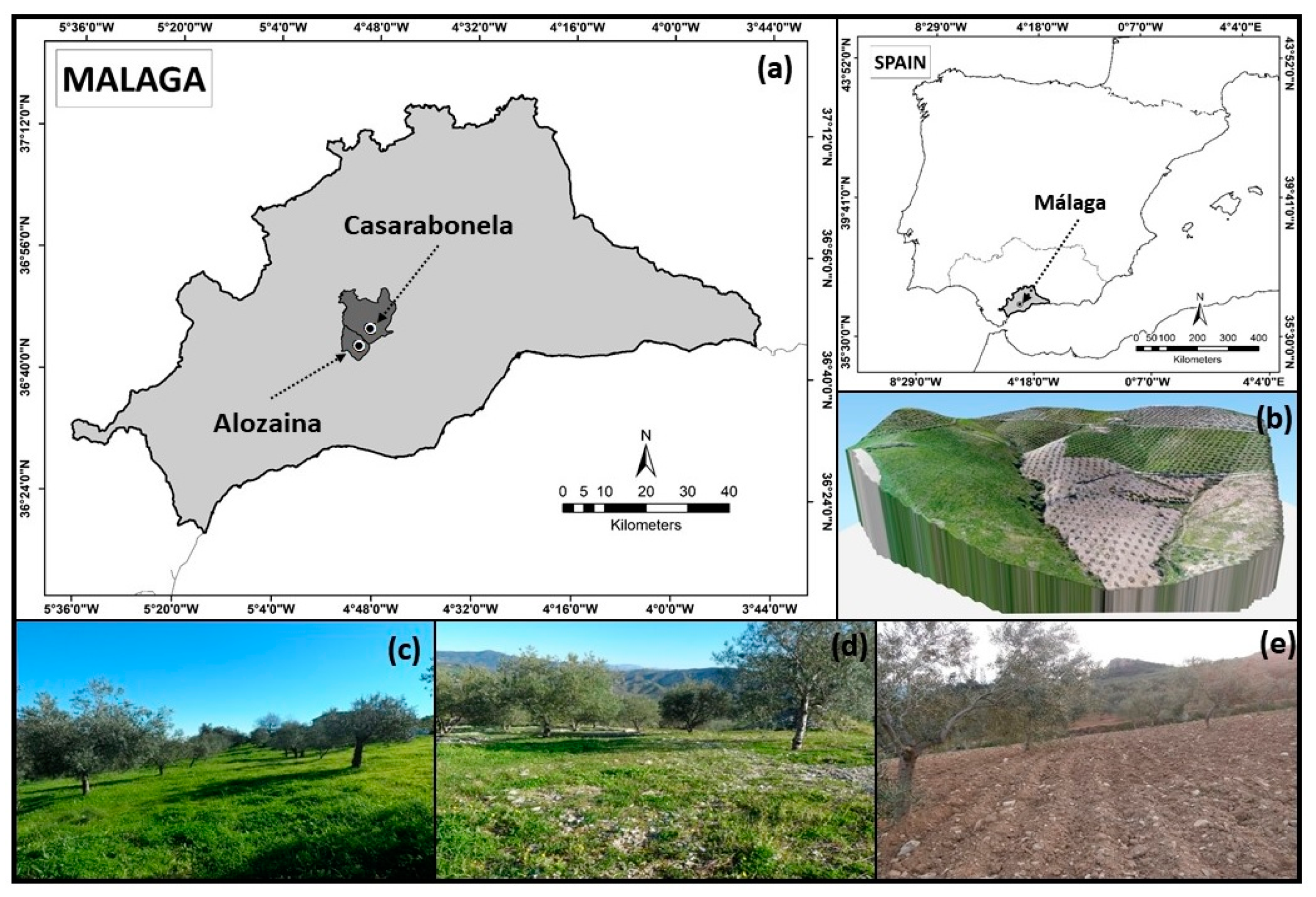
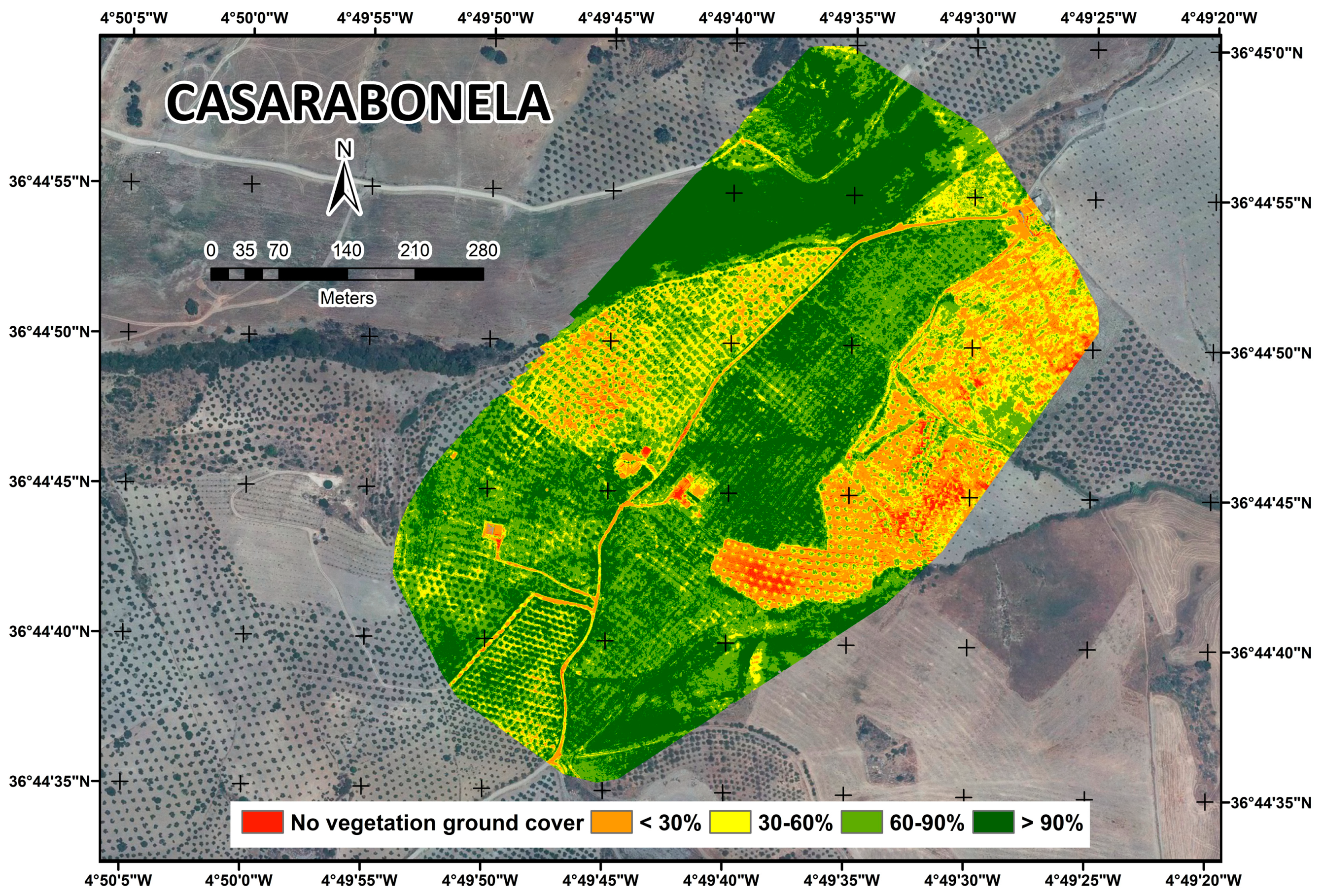
2.1. Study Site

The study was carried out in 57 privately-owned olive groves located in the centre-west of the province of Malaga (southern Spain), in the municipalities of Alozaina (334494,72N, 4064214,89W ETRS 1989 UTM Zone 30N) and Casarabonela (336842, 64N, 4068297.68W ETRS 1989 UTM Zone 30N) (Figure 1a). The relief is undulating (flysch) with slopes ranging 7–30% (Figure 1b).
The predominant soils are Calcic Cambisols, Vertic Cambisols, Calcaric Regosols and Haplic Vertisols [29], with an average depth of 66.4 ± 30.9 cm and an average organic carbon content of 20.3 ± 13.5 g kg−1.
The climate is temperate Mediterranean, with an average annual temperature of 18.4° C and mean annual precipitation of 636 mm. There is a period of prolonged water deficit, from April to September, which, together with the type of soil and its management, influence the development and seasonality of the VGC. These circumstances mean that the density of land cover is highly variable during the year (Figure 1c–e), with a vertical development that varies depending on the species, but in no case exceeds 1 m in height, as it is eliminated beforehand by the farmer. The VGC is mainly composed of grasses, together with weeds and ruderal nitrophytes of the Ruderali-Secalietea class. The Thero-Brometalia order is represented by species such as Aegilops triuncialis, Bromus spp. and Inula viscosa, while examples of the Chenopodietalia order (found in more nitrified environments) include species such as Hordeum murinum and Malva sylvestris, especially in compact surface soils, and Chenopodium album where there is more humidity and a high concentration of nitrogen [30].
Olive trees are cultivated in non-irrigated land, in geometric planting frameworks with 8–10 m between each tree, which provides an average density of 160 trees per hectare (Figure 1b). VGC is managed by means of deep (15–20 cm) and continuous mouldboard ploughing (2–3 times per year), beginning in January and continuing until June. As a result, the soil is bare for most of the year (Figure 1e), except for periods between ploughing operations, especially in the spring, which is when the VGC quickly returns (Figure 1c,d).

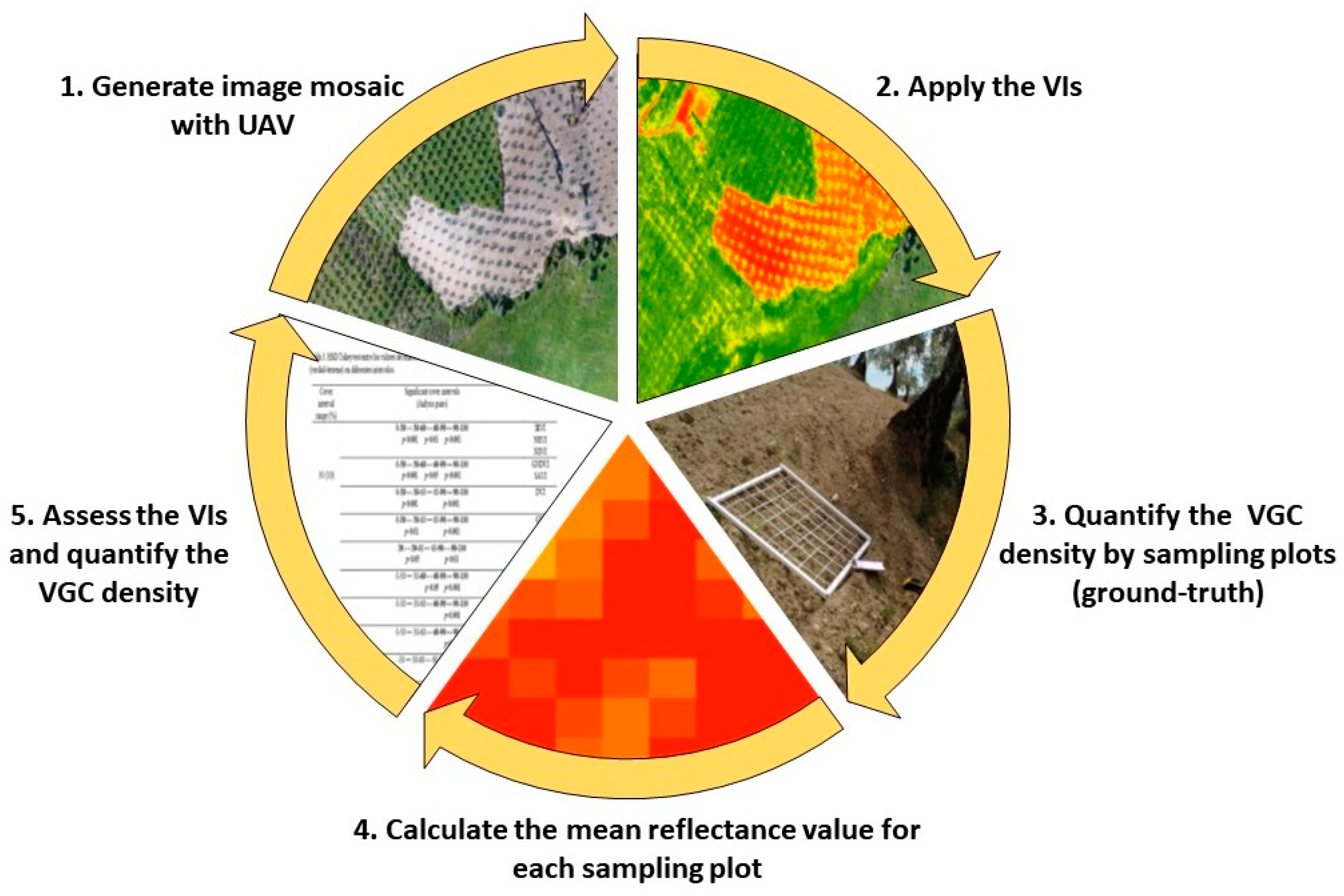
2.2. Quantifying the VGC Density

VGC density is the amount of vegetal cover present on the ground surface. As a preliminary step to quantifying the VGC, a field survey was carried out in each farm and the owners were interviewed to characterise the form of VGC management employed and determine the most appropriate time to perform the UAV flights and obtain the aerial images. The ideal time for this was considered to be mid-April (early spring), when the VGC presented greater variability of surface density, having been present in some cases for several months, giving rise to dense coverage (Figure 1c), while, in other plots, recently cleared, the soil was bare or had only minimal VGC (Figure 1e).
The flights were performed on 16 April at an altitude of 85 m in Alozaina and 90 m in Casarabonela. The difference in altitude was to ensure the safety of the device, because the relief is more abrupt in the Casarabonela farms. As a result of this difference, there was a slight variation in the spatial resolutions obtained (mean ground sampling distance), which were 10.11 cm/pixel and 11.18 cm/pixel in the Alozaina and Casarabonela images, respectively. This difference in altitude had no impact on the study results, as has been reported previously [16].
The method used to quantify VGC consisted of the following steps (Figure 2): (1) conduct the UAV flights and generate image mosaics; (2) apply the VIs; (3) quantify the VGC density by means of sampling plots (SP) (ground-truth); (4) calculate the mean reflectance value of the spectral bands and the VIs in the SPs; and (5) assess the VIs in order to quantify the density of the VGC.

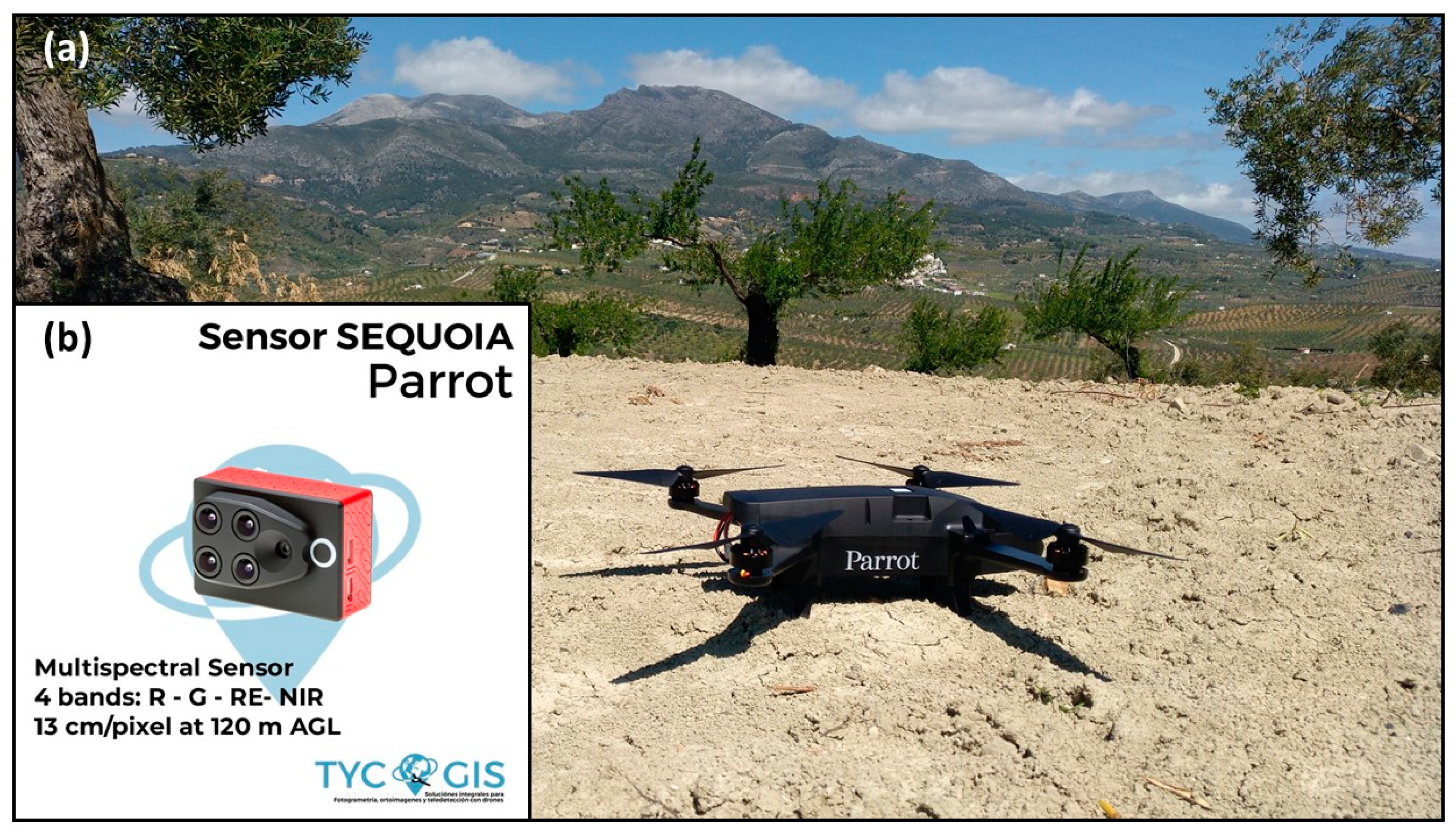
2.2.1. UAV Flights and Image Mosaicking

The images required for this study were obtained using a Parrot Bluegrass quadcopter (Parrot S. A, Paris, France) (Figure 3a), with vertical take off and landing. This device carries a Parrot Sequoia multispectral sensor (Parrot S. A, Paris, France) (Figure 3b), composed of four single-band global shutter cameras with a resolution of 1.2 Mpx (1280 × 960 pixels), capable of capturing four spectral bands in visible and invisible infrared light: Green (G), Red (R), Red Edge (RE), and Near Infrared (NIR). In addition, it has a brightness sensor that records the light conditions, the GPS location and inertial data.
In each flight mission, a sequence of overlapping images (30% side-lap and 60% forward-lap) was taken of each farm in the study area. Pix4Dmapper Pro software, version 4.2.25 (Pix4D S. A, Prilly, Switzerland), was used for the mosaicking and for the radiometric calibration of the images. First, the overall orthomosaic reflectance was obtained for each band. These values were then spectrally corrected by applying an empirical linear relationship [31] from the light sensor data and from the reference photographs taken of the calibrated reflectance panel (Diana Parrot Sequoia 19 cm × 13.5 cm). The geometric calibration was obtained using the GPS parameters and the inertial measurement units from the sensor.

2.2.2. Application of the Vegetation Indices (VIs)

We selected the VIs based on two criteria. Firstly, if they used some of the four bands (G, R, RE and NIR) offered by the multispectral camera used in the flights in their calculations, they were selected. Secondly, the scientific literature has shown that the behaviour of the IVs is variable depending on the existing density of ground cover. Thus, some indices have provided better results when they have been applied in an area with high vegetation ground cover density, while others have responded better in areas with low cover. Taking into account the high heterogeneity of the VGC present in the study area, varied indices were selected to assess their responses to this situation.
The VIs used can be classified as conventional ratio or differential indices (IRVI, RVI, DVI, GVI, GRVI and VREI), indices corrected and derived from the traditional indicators (normalised difference vegetation indices) (NDVI, NRDE, NRVI and GNDVI) and soil reflectance adjusted indices (SAVI) (Table 1).

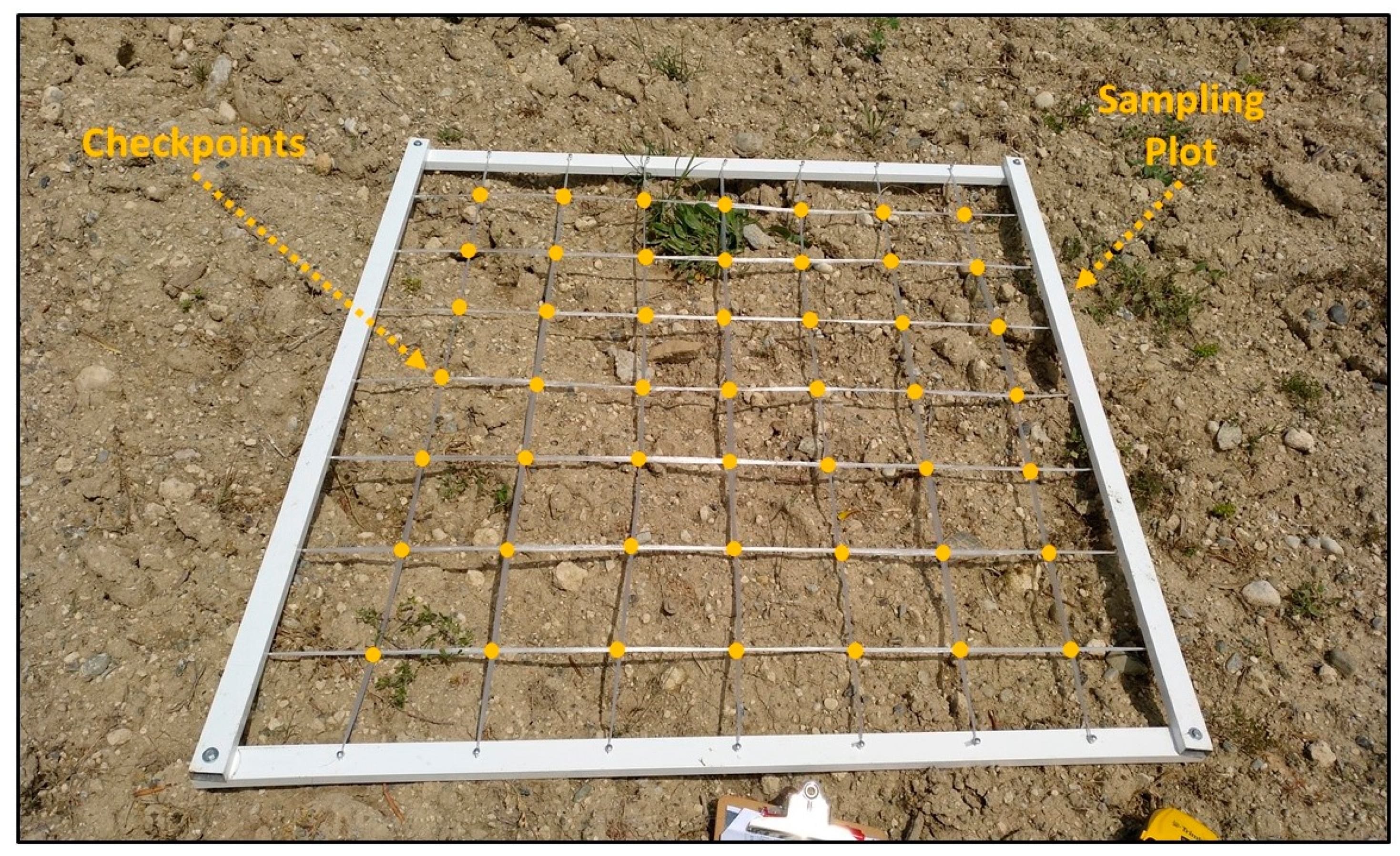
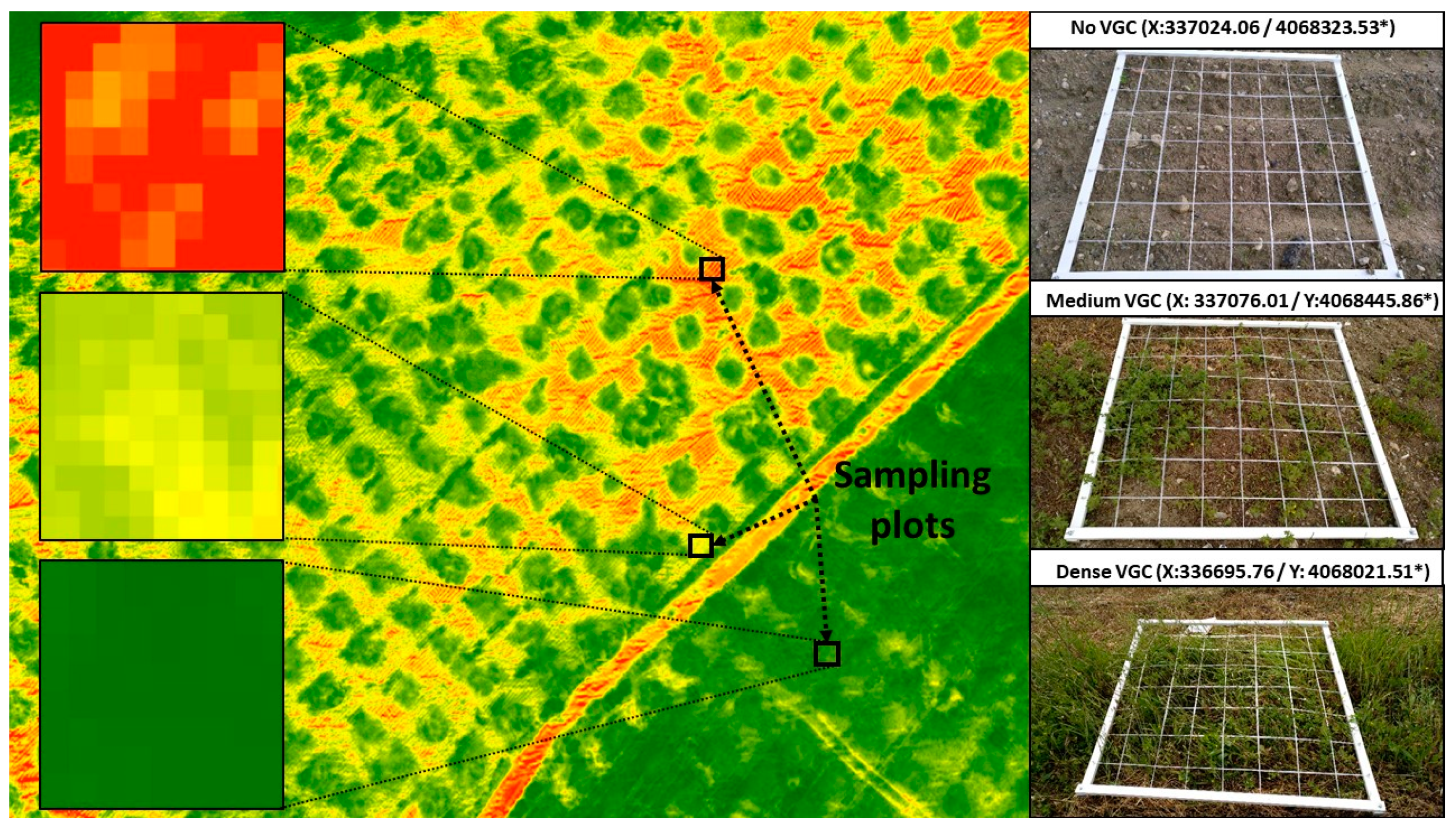
2.2.3. Quantifying VGC Density by Means of Sampling Plots (Ground-Truth)

VIs provide an abstract number that reproduces, in each pixel, the relationship between the bands used. These results must then be related to the real level of ground cover. To do so, a ground-truth field quantification survey of VGC density was performed in 115 sampling plots (SP), distributed randomly (1 SP per 0.5 ha of surface). No samples were taken in areas close to the tree canopies in order to avoid the influence of shade. With a surface area of 1 m2, each SP was divided into quadrants measuring 12.5 cm × 12.5 cm, which provided 49 checkpoints per SP (Figure 4) in which the VGC was quantified by the binary classes “vegetation present” and “vegetation absent”.
The SPs were located in the field using a Trimble Geo XH 6000 real-time decimetric precision GPS collector (10 cm DGNSS real-time accuracy) (Trimble GeoSpatial, Munich, Germany).

2.2.4. Calculating the Mean Reflectance Values of the Spectral Bands and the Vis in the Sampling Plots

The mean reflectance value of the spectral bands and the VIs in each SP was then calculated (Figure 5). Due to the above-discussed differences in spatial resolution, in the Alozaina farms, each SP contained 98 pixels, while in those in Casarabonela there were 80 pixels per SP.

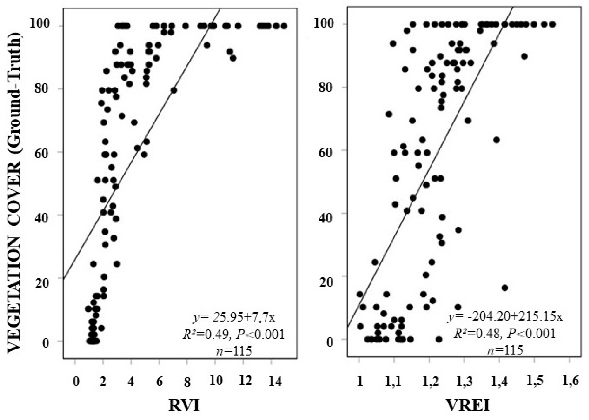
2.2.5. Assessing the VIs to Quantify the VGC Density

The relationship among the spectral bands, the VIs and the ground-truth data was determined by linear regression analysis (stepwise method). We then determined how well the VIs differentiated VGC density at different ranges, using analysis of the variance (ANOVA) and Tukey’s honestly-significant-difference (HSD) test. All statistical analyses were performed using IBM SPSS Statistics 25.0.

3. Results

Regression analysis between the reflectance of the spectral bands used alone and the VGC density shows that the R and G wavelengths have a greater explanatory capacity (R2 = 0.58 and R2 = 0.50, p < 0.001, respectively) than the NIR and RE bands (R2 = 0.33 and R2 = 0.17, p < 0.001, respectively) (Table 2). Multiple regression analysis significantly improves the results when the R and NIR bands are combined (adjusted R2 = 0.74, p < 0.001). The equation with the R, NIR and G bands has the same explanatory capacity (Table 2).
Application of the VIs substantially improves the results. IRVI, NDVI and NRVI provide the most accurate estimates of VGC density (R2 > 0.81, p < 0.001) (Figure 6).
Analysis of the capability of VIs to differentiate intervals of VGC densities highlighted the existence of important differences. Cover interval range is the reference value taken to establish the VGC density. The increase in the range in which the VGC density intervals are expressed was directly proportional to the separability of the VIs (Table 3). For a 10% cover interval range, Tukey’s HSD test shows that RVI (p < 0.001); DVI, GVI and SAVI (p < 0.01); and NRVI and NDVI (p < 0.05) are the only VIs with the ability to differentiate VGC densities > 80%. Lower VGC densities are not differentiated by any of the VIs used.
Increasing the cover interval range to 15% raises the number of indices capable of differentiating VGC densities greater than 75% and, at the same time, improves the accuracy of those that were already significant in the previous interval (10%) (Table 3). Thus, in addition to the high level of significance already found for RVI (p < 0.001), NRVI, NDVI, SAVI, DVI and GVI are now significant. Moreover, new significant indices appear: GNDVI (p < 0.001), IRVI (p < 0.01) and VREI (p < 0.05). In this range, too, we observe the first indices capable of differentiating VGC densities below 30%, namely IRVI (p < 0.01) and NRVI, NDVI and GNDVI (p < 0.05). On the other hand, VGC densities between 30% and 75% remain undifferentiated.
The results obtained for VGC intervals of 20–25% are similar to those for the lower value (15%). New indices (NDRE and GRVI) are capable of differentiating VGC densities greater than 60% and 75%, respectively (Table 3). With VGC densities below 40% and 50%, respectively, the VIs found to be significant in the previous cover interval range (IRVI, NRVI, NDVI and GNDVI) become even more significant (p < 0.001), and further indices become significant, i.e., SAVI (p < 0.01) and NDRE (p < 0.05). VGC densities of 40–60% and 25–75%, respectively, continue to be undifferentiated. Only when the cover interval range reaches 30% do IRVI, NRVI and NDVI (p < 0.01) and GNDVI and SAVI (p < 0.05) discriminate the complete series of VGC density intervals (Table 3).
Figure 7 and Figure 8 show the quantification of the VGC from the application of the regression equation obtained by IRVI. In both figures, the heterogeneity of VGC densities of the study area is clearly observed, which denotes the existence of different temporality in the management of the soil by farmers.
Lima et al. [8] showed for the study area that zones in which the VGC is non-existent or very scarce (with percentages below 30%) correspond to areas ploughed later (early April), when normally they are ploughed in March. For this reason, on the date of the flight (mid-April), the lands were recently ploughed and, therefore, the soil had little vegetation cover. However, the areas that present VGC intervals greater than 60% are those that have not yet were ploughed, which has allowed the ground cover development, taking into account that the last ploughing was approximately in the months of January and February. All these temporality differences in soil management, an aspect that is normal in situations of real use outside the controlled conditions of experimental farmland, increase the demands on the VGC detection and quantification system.

4. Discussion

According to the study results obtained, VIs can be used to quantify VGC density, increasing the vegetation reflectance information obtained by the spectral bands alone. The IRVI, NDVI and NRVI provide the most accurate estimates of VGC density (R2 > 0.81, p < 0.001) in the study area. Although these VIs obtain very similar values, the best result is obtained with IRVI (R2 = 0.82, p < 0.001). The ability of this index to measure green herbaceous biomass at the end of the rainy season was reported by Verbesselt et al. [43]. In the present analysis, we show that the results obtained by the inverse indices such as IRVI are substantially better than those from simple indices such as RVI (R2 = 0.49, p < 0.001). The remaining simple VIs (DVI, GVI and VREI) present the lowest values, and only account for 48–67% of VGC variability.
The corrected indices derived from traditional indicators are also interesting. Normalisation substantially improves the results of the VIs. One example of this improvement is that of NDVI (R2 = 0.81, p < 0.001). This same index, without normalisation (i.e., DVI), is less able to distinguish VGC (R2 = 0.67, p < 0.001). The difference is even more apparent with NRVI (R2 = 0.81, p < 0.001), which prior to normalisation (RVI) had a 32% poorer explanatory capability (R2 = 0.49, p < 0.001). These results are consistent with those obtained by Carlson and Ripley [44] and by Hassan et al. [45], who obtained good results with normalised indices, such as NDVI, to estimate the fraction of vegetation cover. Index normalisation usually improves the results obtained because it provides a greater separation of the green vegetation from its background soil brightness [34] and reduces the effects produced by topographic, atmospheric and lighting factors [10].
The soil reflectance adjusted index (SAVI) is not among the best-performing indices (R2 = 0.77, p < 0.001), because the study area considered has a predominance of areas with high cover density (in 44% of the SP the VGC was greater than 80%) and this VI was designed to analyse areas with little vegetation cover [40].
In our study, the VGC is best quantified by the VIs based on the R and NIR bands, due to the spectral behaviour of the vegetation; the chlorophyll absorbs a greater proportion of the electromagnetic waves in the R region, and high reflectance values are observed in the NIR region due to the microcellular structures of the leaf material [46].
However, this is not the case with the VIs derived from the G or RE bands. While the G band, used individually, obtains an acceptable result (R2 = 0.50, p < 0.001), its incorporation into the VIs worsens their performance. This deterioration is apparent with GNDVI (R2 = 0.79, p < 0.001) and even more so with GRVI (R2 = 0.52, p < 0.001), with respect to NDVI (R2 = 0.81, p < 0.001). Both of these VIs perform worse when the G band replaces the R band (GNDVI) or the NIR band (GRVI). These results corroborate those of Khajeddin [14] and Barati et al. [47], who reported that the use of the G band reduces the sensitivity of the VIs.
The RE band, used individually, does not obtain good results (R2 = 0.17, p < 0.001). This is reflected in the VIs that incorporate this band, such as VREI (R2 = 0.48, p < 0.001) and NDRE (R2 = 0.50, p < 0.001). From these results, we conclude that VIs based on the RE band are relatively insensitive to the quantification of VGC, although Dong et al. [48] stated that RE-based VIs are more sensitive to chlorophyll and can be used to derive an empirical model for estimating the leaf area index in different crops.
As expected, the behaviour of the VIs in response to different VGC densities is not homogeneous, but improves in line with the increase in cover interval ranges. Tukey’s HSD test shows that the most suitable indices to quantify areas with VGC densities greater than 80%, at a cover interval range of 10%, are RVI (p < 0.001); DVI, GVI and SAVI (p < 0.01); and NRVI and NDVI (p < 0.05). NDRE and VREI are expected to obtain very similar results, since these indices are normally more robust and perform better in areas of greater canopy density [49], and hence no saturation deficiencies [50,51,52]. These VIs begin to be significant (p < 0.05) at a cover range of 15% (VREI) and 20% (NDRE).
For the discrimination of areas with a VGC density of less than 30%, IRVI (p < 0.01) is the most significant at a cover interval range of 15%. Its estimation capacity decreases as the biomass increases, since the greater is the biomass, the lower is the reflectance of the R band and the greater is the reflectance of the NIR band [43].
IRVI, NRVI and NDVI (p < 0.001 and p < 0.01) and GNDVI and SAVI (p < 0.001 and p < 0.05) only achieve a significant differentiation at all coverage intervals within the same range when the cover interval range reaches 30%. From these results, we conclude that VIs are especially useful for detecting and quantifying homogeneous surfaces, such as areas that are either completely covered or have very little vegetation cover. However, when the VGC is slight or moderate, the reflectance measured does not depend exclusively on the vegetation cover, but also on other factors, such as the soil. The VI is then a less precise instrument. As mentioned above, the analysis of land cover in woody crops, such as olive groves, tends to generate high error rates in remote sensing. In the present study, the differentiation capacity of the VIs was severely tested by their use in a region of very heterogeneous soil cover; some of the olive groves had not been cleared for several months and so the VGC was quite dense, while in others the soil was bare, and subjected to diverse soil management regimes (tillage vs. no tillage). In this context, it can be considered normal that some of the VIs were only able to significantly differentiate all vegetation cover intervals with the same range above a cover interval range of 30%. Better results are to be expected for crops or areas in which the ground cover is more homogeneous.

5. Conclusions

In this paper, we show that UAV technology, together with image processing based on VIs, makes it possible to remotely quantify the density of VGC produced spontaneously in olive groves. Of the 11 VIs considered, IRVI was the most sensitive to quantify VGC density at intervals of 10–25%. Only when the cover interval range rose to 30% did IRVI, NRVI, NDVI, GNDVI and SAVI differentiate the complete series of densities.
The study described in this paper provides: (a) a better understanding of the behaviour of VIs in response to different soil cover densities; (b) a demonstration of the ability to remotely quantify the VGC in olive groves with heterogeneous soil cover; (c) a contribution to providing control and monitoring tools enabling recipients of CAP benefits to comply with cross-compliance requirements in terms of minimum soil cover; and (d) to know the temporality of the operations carried out in the soil, which is of great importance to adapt this to the rainfall conditions of the area, and avoid the existence of bare soils in the periods of more intense rainfall.
However, due to the dynamic, heterogeneous nature of the VGC in olive groves, further research is needed in this area, applying the method to images obtained in other seasons (i.e., in summer, autumn and winter), and in regions where there is less ground cover heterogeneity.

Author Contributions

F.J.L.-C. designed and processed the research and drafted the manuscript; F.J.L.-C., R.B.-S., and M.L.G.-M. worked on contextualising the document; F.J.L.-C. and R.B.-S. determined the approach taken to the study methodology, formal analysis and validation; and F.J.L.-C., R.B.-S., M.L.G.-M. and F.B.G.-J. played an active role in writing, reviewing and editing the manuscript. All authors contributed substantially to the paper.

Funding

This study was conducted within the framework of a predoctoral contract (A.2) under the I Research and Transfer Plan of the University of Málaga, and was also funded by the University of Málaga through the mode B3 of assistance for research projects.

Acknowledgments

Invaluable cooperation was provided by the farmers of the lower Guadalhorce Valley-Sierra de las Nieves and by the company TYC-GIS Soluciones Integrales (http://tycgis.com/), to whom we express our gratitude.

Conflicts of Interest

The authors declare they have no conflict of interest.

References

  1. FAO. Food and Agriculture Organization of the United Nations, FAOSTAT. 2016. Available online: http://www.fao.org/faostat/es/#data/QC (accessed on 6 September 2018).
  2. INE. National Institute of Statistics of Spain. Agrarian Census. 2009. Available online: https://www.ine.es/dyngs/INEbase/es/operacion.htm?c=Estadistica_C&cid=1254736176851&menu=resultados&secc=1254736194950&idp=1254735727106 (accessed on 6 September 2018).
  3. Infante, J. The ecology and history of the Mediterranean olive grove: The Spanish great expansion, 1750–2000. Rural Hist. 2012, 23, 161–184. [Google Scholar] [CrossRef]
  4. Lima-Cueto, F.J.; Gómez-Moreno, M.L.; Blanco-Sepúlveda, R. Mountain olive groves and soil preservation in the transition from an organic to an industrial economy: The case of Sierra de las Nieves (Málaga, Spain), 1940–1975. J. Depopulation Rural Dev. Stud. 2017, 23, 97–128. [Google Scholar]
  5. Moreno, B.; García-Rodriguez, S.; Cañizares, R.; Castro, J.; Benítez, E. Rainfed olive farming in south-eastern Spain: Long-term effect of soil management on biological indicators of soil quality. Agric. Ecosyst. Environ. 2009, 131, 333–339. [Google Scholar] [CrossRef]
  6. Brussaard, L.; Kuyper, T.W.; Didden, W.A.M.; de Goede, R.G.M.; Bloem, J. Biological soil quality from biomass to biodiversity–Importance and resilience to management stress and disturbance. In Managing Soil Quality: Challenges in Modern Agriculture; Schjønning, P., Elmholt, S., Christensen, B.T., Eds.; CAB International: Wallingford, UK, 2004; pp. 139–171. [Google Scholar]
  7. Sastre, B.; Marques, M.J.; García-Díaz, A.; Bienesa, R. Three years of management with cover crops protecting sloping olive groves soils, carbon and water effects on gypsiferous soil. Catena 2018, 171, 115–124. [Google Scholar] [CrossRef]
  8. Lima-Cueto, F.J.; Blanco-Sepúlveda, R.; Gómez-Moreno, M.L. Soil erosion and environmental regulations in the European Agrarian Policy for olive groves (Olea europea L.) of southern Spain. Agrociencia 2018, 52, 293–308. [Google Scholar]
  9. Fang, H.; Liang, S. Leaf Area Index Models. Reference Module in Earth Systems and Environmental Sciences. Encycl. Ecol. 2014, 2139–2148. Available online: https://0-www-sciencedirect-com.brum.beds.ac.uk/science/article/pii/B9780080454054001907 (accessed on 1 September 2018).
  10. Broge, N.H.; Leblanc, E. Comparing prediction power and stability of broadband and hyperspectral vegetation indices for estimation of green leaf area index and canopy chlorophyll density. Remote Sens. Environ. 2000, 76, 156–172. [Google Scholar] [CrossRef]
  11. Baret, F.; Guyot, G. Potentials and limits of vegetation indices for LAI and APAR assessment. Remote Sens. Environ. 1991, 35, 161–173. [Google Scholar] [CrossRef]
  12. Richardson, A.J.; Wiegand, C.L.; Wajura, D.F.; Dusek, D.; Steiner, J.L. Multisite analyses of spectral-biophysical data for sorghum. Remote Sens. Environ. 1992, 41, 71–82. [Google Scholar] [CrossRef]
  13. Song, W.; Mu, X.; Ruan, G.; Gao, Z.; Li, L.; Yan, G. Estimating fractional vegetation cover and the vegetation index of bare soil and highly dense vegetation with a physically based method. Int. J. Appl. Earth Obs. Geoinf. 2017, 58, 168–176. [Google Scholar] [CrossRef]
  14. Xiao, J.; Moody, A. A comparison of methods for estimating fractional green vegetation cover within a desert-to-upland transition zone in central New Mexico, USA. Remote Sens. Environ. 2005, 98, 237–250. [Google Scholar] [CrossRef]
  15. Barati, S.; Rayegani, B.; Saati, M.; Sharifi, A.; Nasri, M. Comparison the accuracies of different spectral indices for estimation of vegetation cover fraction in sparse vegetated areas. Egypt. J. Remote Sens. Space Sci. 2011, 14, 49–56. [Google Scholar] [CrossRef] [Green Version]
  16. Torres, J.; Peña, J.M.; De Castro, A.I.; Lopez, F. Multi-temporal mapping of the vegetation fraction in early-season wheat fields using images from UAV. Comput. Electron. Agric. 2014, 103, 104–113. [Google Scholar] [CrossRef]
  17. Yun, H.S.; Park, S.H.; Kim, H.J.; Lee, W.D.; Lee, K.D.; Hong, S.Y.; Jung, G.H. Use of unmanned aerial vehicle for multi-temporal monitoring of soybean vegetation fraction. J. Biosyst. Eng. 2016, 41, 126–137. [Google Scholar] [CrossRef]
  18. Peña-Barragán, J.M.; Jurado-Expósito, M.; López-Granados, F.; Atenciano, S.; Sánchez-De la Orden, M.; García-Ferrer, A.; García-Torres, L. Assessing land-use in olive groves from aerial photographs. Agric. Ecosyst. Environ. 2004, 103, 117–122. [Google Scholar] [CrossRef]
  19. García, L.; Peña-Barragán, J.M.; López-Granados, F.; Jurado-Expósito, M.; Fernández-Escobar, R. Automatic assessment of agro-environmental indicator from remotely sensed images of tree orchards and its evaluation using olive plantions. Comput. Electron. Agric. 2008, 61, 179–191. [Google Scholar] [CrossRef]
  20. Torres-Sánchez, J.; López-Granados, F.; Serrano, N.; Arquero, O.; Peña, J.M. High-throughput 3-d monitoring of agricultural-tree plantations with unmanned aerial vehicle (UAV) technology. PLoS ONE 2015, 10, e0130479. [Google Scholar] [CrossRef] [PubMed]
  21. Avola, G.; Di Gennaro, S.F.; Cantini, C.; Riggi Ezio Muratore, F.; Tornambe, C.; Matese, A. Remotely sensed vegetation indices to discriminate field-grown olive cultivars. Remote Sens. 2019, 11, 1242. [Google Scholar] [CrossRef]
  22. De Castro, A.I.; Six, J.; Plant, R.E.; Peña, J.M. Mapping Crop Calendar Events and Phenology-Related Metrics at the Parcel Level by Object-Based Image Analysis (OBIA) of MODIS-NDVI Time-Series: A Case Study in Central California. Remote Sens. 2018, 10, 1745. [Google Scholar] [CrossRef]
  23. Pinilla, C.; Ariza, F.J.; Sánchez, M.; Tovar, J. Improvement of the reliability in the identification of the olive grove using a geometric reflectance model. J. Remote Sens. 2001, 16, 11–15. (In Spanish) [Google Scholar]
  24. Huete, A.R.; Jackson, R.D.; Post, D.F. Spectral response of a plant canopy with different soil backgrounds. Remote Sens. Environ. 1985, 17, 37–53. [Google Scholar] [CrossRef]
  25. Iaquinta, J.; Fouilloux, A. Influence of the heterogeneity and topography of vegetated land surfaces for remote sensing applications. Int. J. Remote Sens. 1988, 19, 1711–1723. [Google Scholar] [CrossRef]
  26. Saberioon, M.M.; Amin, M.S.M.; Anuar, A.R.; Gholizadeh, A.; Wayayok, A.; Khairunniza-Bejo, S. Assessment of rice leaf chlorophyll content using visible bands at different growth stages at both the leaf and canopy scale. Int. J. Appl. Earth Obs. Geoinf. 2014, 32, 35–45. [Google Scholar] [CrossRef]
  27. De Castro, A.I.; Jiménez-Brenes, F.M.; Torres-Sánchez, J.; Peña, J.M.; Borra-Serrano, I.; López-Granados, F. 3-D Characterization of Vineyards Using a Novel UAV Imagery-Based OBIA Procedure for Precision Viticulture Applications. Remote Sens. 2018, 10, 584. [Google Scholar] [CrossRef]
  28. Catur, A.R. The potential of UAV-based remote sensing for supporting precision agriculture in Indonesia. Procedia Environ. Sci. 2015, 24, 245–253. [Google Scholar]
  29. FAO. World Reference Base for Soil Resources 2014. International Soil Classification System for Naming Soils and Creating Legends for Soil Maps. Update 2015; Food and Agriculture Organization of the United Nations: Rome, Italy, 2014; ISSN 0532-0488. [Google Scholar]
  30. Foraster, L.; Gómez, E.J.; Iglesias, I.; Macías, F.J.; Ruiz, M. Study for the Delimitation of Experimental Zones. Olive Grove of the Sierra de Las Nieves Region. Characterization and Recommendations for Ecological Management; Mancomunidad de Municipios Sierra de las Nieves: Málaga, Spain, 2011; ISBN 978-84-930235-5-4. (In Spanish) [Google Scholar]
  31. Hunt, E.R.; Hively, W.D.; Fujikawa, S.J.; Linden, D.S.; Daughtry, C.S.T.; McCarty, G.W. Acquisition of NIR-green–blue digital photographs from unmanned aircraft for crop monitoring. Remote Sens. 2010, 2, 290–305. [Google Scholar] [CrossRef]
  32. Richardson, A.J.; Wiegand, C.L. Distinguishing vegetation from soil background information. Photogramm. Eng. Remote Sens. 1977, 43, 1541–1552. [Google Scholar]
  33. Birth, G.S.; Birth, G.R. Measuring the color of growing turf with a reflectance spectrophotometer. Am. Soc. Agron. 1968, 60, 640–643. [Google Scholar] [CrossRef]
  34. Rouse, J.W.; Haas, R.H.; Schell, J.A.; Deering, D.W. Monitoring vegetation systems in the Great Plains with ERTS. In Third Earth Resources Technology Satellite–1 Syposium; Freden, S.C., Mercanti, E.P., Becker, M., Eds.; Technical Presentations, NASA SP-351; NASA: Washington, DC, USA, 1973; Volume 1, pp. 309–317. [Google Scholar]
  35. Gitelson, A.A.; Kaufman, Y.J.; Merzlyak, M.N. Use of a green channel in remote sensing of global vegetation from EOS-MODIS. Remote Sens. Environ. 1996, 58, 289–298. [Google Scholar] [CrossRef]
  36. Gitelson, A.A.; Merzlyak, M.N. Spectral reflectance changes associated with autumn senescence of Aesculus hippocatanum I and Hacer plantanoides I. leaves. Spectral features and relation to chlorophyll estimation. J. Plant Physiol. 1994, 143, 286–292. [Google Scholar] [CrossRef]
  37. Tucker, C.J. Red and photographic infrared linear combinations for monitoring vegetation. Remote Sens. Environ. 1979, 8, 127–150. [Google Scholar] [CrossRef] [Green Version]
  38. Falkowski, M.J.; Gessler, P.E.; Morgan, P.; Hudak, A.T.; Smith, A.M.S. Characterizing and mapping forest fire fuels using ASTER imagery and gradient modeling. For. Ecol. Manag. 2005, 217, 129–146. [Google Scholar] [CrossRef] [Green Version]
  39. Cruden, B.A.; Prabhu, D.; Martinez, R. Absolute radiation measurement in Venus and Mars entry conditions. J. Spacecr. Rocket. 2012, 49, 1069–1079. [Google Scholar] [CrossRef]
  40. Huete, A.R. A soil vegetation adjusted index (Savi). Remote Sens. Environ. 1988, 25, 295–309. [Google Scholar] [CrossRef]
  41. Vogelmann, B.N.; Rock, D.M. Moss Red edge spectral measurements from sugar maple leaves. Int. J. Remote Sens. 1993, 14, 1563–1575. [Google Scholar] [CrossRef]
  42. Richardson, A.; Everitt, J. Using spectral vegetation indices to estimate rangeland productivity. Geocarto. Int. 1992, 1, 63–77. [Google Scholar] [CrossRef]
  43. Verbesselt, J.; Somers, B.; Van Aardt, J.; Jonckheere, I.; Coppin, P. Monitoring herbaceous biomass and water content with spot vegetation time-series to improve fire risk assessment in savanna ecosystems. Remote Sens. Environ. 2006, 101, 399–414. [Google Scholar] [CrossRef]
  44. Carlson, D.A.; Ripley, D.A. On the relation between NDVI, fractional vegetation cover, and leaf area index. Remote Sens. Environ. 1997, 62, 241–252. [Google Scholar] [CrossRef]
  45. Hassan, M.A.; Yang, M.; Rasheed, A.; Yang, G.; Reynolds, M.; Xia, X.; Xiao, Y.; He, Z. A rapid monitoring of NDVI across the wheat growth cycle for grain yield prediction using a multi-spectral UAV platform. Plant Sci. 2019, 282, 95–103. [Google Scholar] [CrossRef]
  46. Tucker, C.J. A spectral method for determining the percentage of green herbage material in clipped samples. Remote Sens. Environ. 1980, 9, 175–181. [Google Scholar] [CrossRef]
  47. Khajeddin, S.J. A Survey of the Plant Communities of the Jazmorian, Iran, Using Landsat MSS Data; Reading University: Reading, UK, 1995. [Google Scholar]
  48. Dong, T.; Lui, J.; Shang, J.; Qian, B.; Ma, B.; Kovacs, J.M.; Walters, D.; Jiao, X.; Geng, X.; Shi, Y. Assessment of red-edge vegetation indices for crop leaf area index estimation. Remote Sens. Environ. 2019, 222, 133–143. [Google Scholar] [CrossRef]
  49. Mutanga, O.; Skidmore, A.K. Narrow band vegetation indices overcome the saturation problem in biomass estimation. Int. J. Remote Sens. 2004, 25, 3999–4014. [Google Scholar] [CrossRef]
  50. Huete, A.; Didan, K.; Miura, T.; Rodriguez, E.P.; Gao, X.; Ferreira, L.G. Overview of the radiometric and biophysical performance of the MODIS vegetation indices. Remote Sens. Environ. 2002, 83, 195–213. [Google Scholar] [CrossRef]
  51. Eitel, J.U.H.; Vierling, L.A.; Litvak, M.E.; Long, D.S.; Schulthess, U.; Ager, A.A.; Krofcheck, D.J.; Stoscheck, L. Broadband, red-edge information from satellites improves early stress detection in a New Mexico conifer woodland. Remote Sens. Environ. 2011, 115, 3640–3646. [Google Scholar] [CrossRef]
  52. Marx, A. The Impact of the RapidEye Red Edge Band in Mapping Defoliation Symptoms; ESA Living Planet Symposium: Edinburgh, UK, 2013; Available online: http://seom.esa.int/LPS13/5405ddfb/ (accessed on 1 July 2017).
Figure 1. Study area: (a) location in the province of Malaga; (b) undulating relief and geometric planting framework; (c) areas with high VGC density; (d) areas with medium VGC density; and (e) no VGC (bare soil).
Remotesensing 11 02564 g001
Figure 2. Stages of the method used to quantify the density of vegetation ground cover (VGC).
Remotesensing 11 02564 g002
Figure 3. UAV quadcopter (a) and multispectral sensor (b).
Remotesensing 11 02564 g003
Figure 4. Quadrant-based method for quantifying VGC.
Remotesensing 11 02564 g004
Figure 5. Random distribution of the sampling plots within the NDVI image (centre), detail of the pixels constituting the average NDVI reflectance value for each SP (left), ground-truth (right) (* Coordinate System: ETRS 1989 UTM Zone 30N).
Remotesensing 11 02564 g005
Figure 6. Scatter diagrams and regression curves of the relation between vegetation cover (Ground-Truth) and VIs.
Remotesensing 11 02564 g006aRemotesensing 11 02564 g006b
Figure 7. Quantification map of the VGC in Alozaina, made at a cover interval range of 30 % using IRVI index.
Remotesensing 11 02564 g007
Figure 8. Quantification map of the VGC in Casarabonela, made at a cover interval range of 30% using IRVI index.
Remotesensing 11 02564 g008
Table 1. Vegetation indices applied.
IndexFormula aReference
IRVI (Inverse Ratio Vegetation Index) R N I R [32]
RVI (Ratio Vegetation Index) N I R R [33]
DVI (Difference Vegetation Index) N I R R [32]
NDVI (Normalised Difference Vegetation Index) N I R R N I R + R [34]
GNDVI (Green Normalised Difference Vegetation Index) N I R G N I R + G [35]
NDRE (Normalised Difference Red Edge) N I R R E N I R + R E [36]
GRVI (Green-Red Vegetation Index) G R G + R [37,38]
GVI (Green Vegetation Index) N I R G [39]
NRVI (Normalised Ratio Vegetation Index) R V I 1 R V I + 1 [11]
SAVI (Soil-Adjusted Vegetation Index) b N I R R N I R + R + L   ( 1 + L ) [40]
VREI (Vogelmann Rededge Index) N I R R E [41]
a Wavelength band values G (550 nm centre, 40 nm bandwidth), R (660 nm centre, 40 nm bandwidth), RE (735 nm centre, 10 nm bandwidth), NIR (790 nm centre, 40 nm bandwidth). b L= Soil adjustment factor 0.5 for intermediate coverage values [42].
Table 2. Estimating VGC density from spectral bands (n = 115).
BandRegression ModelRR2Adjusted R2P-Value
Ry = 108.05 − 413R0.7650.5840.581p < 0.001
Gy = 135.63 − 659.93G0.7100.5040.500p < 0.001
NIRy = − 14.46 + 217.92NIR0.5710.3260.320p < 0.001
REy = − 6.08 + 237.197RE0.4090.1670.160p < 0.001
R, NIRy = 49.53 − 358.58R + 155.76NIR0.8610.7410.737p < 0.001
R, NIR, Gy = 60.41−161.04R + 173.28NIR−346.05G0.8670.7520.745p < 0.001
G: Green; R: Red; RE: Red Edge; NIR: Near Infrared.
Table 3. Tukey’s HSD test of reflectance values for VIs and ground-truth VGC at different intervals. The table expresses in a range of increasing coverage interval (from 10% to 30%) the separability between coverage intervals for each VI applied. The coverage interval ranges within the parentheses correspond to VGC values greater than 90% because the entire series could not be divided into regular intervals. Bold letters indicate that there is statistically significant separability in coverage intervals, accompanied by the level of significance (p).
Cover Interval Range (%) Significant Cover Intervals (Analysis Pairs)VI
100–10 10–20 20–30 30–40 40–50 50–60 60–70 70–80 80–90 90–100
                                p < 0.001
RVI
0–10 10–20 20–30 30–40 40–50 50–60 60–70 70–80 80–90 90–100
                                p < 0.01
DVI
GVI
SAVI
0–10 10–20 20–30 30–40 40–50 50–60 60–70 70–80 80–90 90–100
                                p < 0.05
NRVI
NDVI
0–10 10–20 20–30 30–40 40–50 50–60 60–70 70–80 80–90 90–100Other VIs
15 (10)0–15 15–30 30–45 45–60 60–75 75–90 90–100
p < 0.01                 p < 0.01
IRVI
0–15 15–30 30–45 45–60 60–75 75–90 90–100
p < 0.05                 p < 0.001
NRVI
NDVI
GNDVI
0–15 15–30 30–45 45–60 60–75 75–90 90–100
                     p < 0.001
RVI
DVI
GVI
SAVI
0–15 15–30 30–45 45–60 60–75 75–90 90–100
                     p < 0.05
VREI
0–15 15–30 30–45 45–60 60–75 75–90 90–100Other VIs
200–20 20–40 40–60 60–80 80–100
p < 0.001        p < 0.001
IRVI
NRVI
NDVI
GNDVI
0–20 20–40 40–60 60–80 80–100
p < 0.01         p < 0.001
SAVI
0–20 20–40 40–60 60–80 80–100
p < 0.05         p < 0.05
NDRE
0–20 20–40 40–60 60–80 80–100
            p < 0.001
RVI
DVI
GVI
0–20 20–40 40–60 60–80 80–100
            p < 0.05
VREI
0–20 20–40 40–60 60–80 80–100Other VIs
250–25 25–50 50–75 75–100
p < 0.001    p < 0.001
IRVI
NRVI
NDVI
GNDVI
SAVI
0–25 25–50 50–75 75–100
p < 0.05    p < 0.001
DVI
NDRE
0–25 25–50 50–75 75–100
        p < 0.001
RVI
GVI
GRVI
VREI
0–25 25–50 50–75 75–100Other VIs
30 (10)0–30 30–60 60–90 90–100
  p < 0.001 p < 0.01 p < 0.001
IRVI
NRVI
NDVI
0–30 30–60 60–90 90–100
  p < 0.001  p < 0.05  p < 0.001
GNDVI
SAVI
0–30 30–60 60–90 90–100
p < 0.001     p < 0.001
DVI
0–30 30–60 60–90 90–100
p < 0.01     p < 0.001
GVI
0–30 30–60 60–90 90–100
p < 0.05    p < 0.01
NDRE
0–30 30–60 60–90 90–100
    p < 0.05 p < 0.001
GRVI
0–30 30–60 60–90 90–100
        p < 0.001
RVI
0–30 30–60 60–90 90–100
        p < 0.01
VREI
0–30 30–60 60–90 90–100Other VIs

