Lifting Scheme-Based Deep Neural Network for Remote Sensing Scene Classification

Abstract

Recently, convolutional neural networks (CNNs) achieve impressive results on remote sensing scene classification, which is a fundamental problem for scene semantic understanding. However, convolution, the most essential operation in CNNs, restricts the development of CNN-based methods for scene classification. Convolution is not efficient enough for high-resolution remote sensing images and limited in extracting discriminative features due to its linearity. Thus, there has been growing interest in improving the convolutional layer. The hardware implementation of the JPEG2000 standard relies on the lifting scheme to perform wavelet transform (WT). Compared with the convolution-based two-channel filter bank method of WT, the lifting scheme is faster, taking up less storage and having the ability of nonlinear transformation. Therefore, the lifting scheme can be regarded as a better alternative implementation for convolution in vanilla CNNs. This paper introduces the lifting scheme into deep learning and addresses the problems that only fixed and finite wavelet bases can be replaced by the lifting scheme, and the parameters cannot be updated through backpropagation. This paper proves that any convolutional layer in vanilla CNNs can be substituted by an equivalent lifting scheme. A lifting scheme-based deep neural network (LSNet) is presented to promote network applications on computational-limited platforms and utilize the nonlinearity of the lifting scheme to enhance performance. LSNet is validated on the CIFAR-100 dataset and the overall accuracies increase by 2.48% and 1.38% in the 1D and 2D experiments respectively. Experimental results on the AID which is one of the newest remote sensing scene dataset demonstrate that 1D LSNet and 2D LSNet achieve 2.05% and 0.45% accuracy improvement compared with the vanilla CNNs respectively.

1. Introduction

1.1. Background

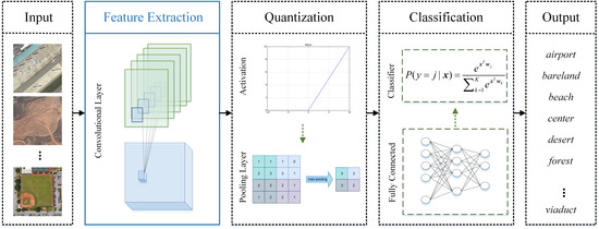
High-resolution remote sensing images contain complex geometrical structures and spatial patterns and thus scene classification is a challenge for remote sensing image interpretation. Discriminative feature extraction is vital for scene classification which aims to automatically assign a semantic label to each remote sensing image to know the category it belongs to. Recently, convolutional neural networks (CNNs) has attracted increasing attention in remote sensing community [1,2], which can learn more abstract and discriminative features and achieve the state-of-the-art performance on classification. A typical CNN framework is shown in Figure 1, where three types of modules are cast into, including feature extraction module, quantization module, and trick module. The quantization module includes spatial quantization, amplitude quantization, and evaluation quantization. Pooling is a typical spatial quantization used for downsampling and dimensionality reduction to reduce the number of parameters and calculations while maintaining significant information. Amplitude quantization is a nonlinear process that compresses real values into a specific range. Examples are sigmoid, tanh, ReLU [3] and its variants [4,5,6], which are often used to activate neurons because nonlinearity is vital for strengthening the approximation and representation abilities. Evaluation quantization is performed to obtain the outputs that meet the specific requirements. For instance, the softmax function is often used in the final hidden layer of a neural network to output classification probabilities. The trick module contains some algorithms such as dropout [7] and batch normalization [8], for improving training effects and achieving better performance. Among all the modules, the feature extraction module is the most essential, which is based on convolution to extract image features. It invests CNN with some favourable characteristics such as local perception, parameter sharing, and translation invariance.

The extraction of scene-level discriminative features is the key step of scene classification. In CNN-based methods, convolution is the most critical technology for remote sensing imagery feature extraction. It has the properties of local connection, weight sharing, and translation invariance, which makes full use of the spatial relationship between pixels. However, convolution has some intrinsic drawbacks, such as considerable computational complexity and limitation in transformation capacity due to its linearity. For high-resolution remote sensing images, the computation challenge is severe, and the considerable computational complexity restrains scene classification from that conducted on computationally limited hardware platforms. In addition, it is vital to learn discriminative feature representation of remote sensing images, but the linearity impedes CNNs from extracting more powerful features with better representation and fitting well on complex functions. To extract more representative features, the literature [9] employs collaborative representation after a pre-trained CNN. The literature [10] integrates multilayer features of CNNs. In [11], the last two fully connected layer features of pre-trained VggNet are fused to improve the discriminant ability. In [12], the pre-trained deep CNN is combined with a sparse representation to improve the performance. Most of these methods increase the dimension of features and none of them are proposed to improve the convolutional layer. Therefore, exploration for a better method to extract features is still of great significance for future CNN-based scene classification research.

Convolution is also the paramount operation of the traditional implementation of the wavelet transform (WT). The discrete wavelet transform (DWT) is one branch of WT, which is traditionally implemented by the two-channel filter bank representation [13]. It is widely applied in scientific fields because it has the favourable characteristic of time-frequency localization, but is limited by the considerable computation complexity and the linearity brought by convolution. To overcome those difficulties, W. Sweldens proposed the lifting scheme [14,15,16,17,18], which mainly contains three steps: split, predict, and update. Split: The input signal is decomposed into two non-overlapping sample sets. A common method is the lazy wavelet transform, which splits the original signal into an even subset and an odd subset, both of which contain half the number of input samples. Predict: The two subsets divided by a signal with strong local correlation are highly correlated in most cases. With one subset known, another subset is reasonably predicted with some predicted error produced. In particular, the predicted errors are all zero for a constant signal. Update: One key characteristic of coarse signals is that they have the same average as the input signal, which is guaranteed by this step. The lifting scheme is an efficient algorithm for traditional DWT as Daubechies and W. Sweldens proved that any FIR wavelet transform can be decomposed into a series of prediction and update steps [19]. The form of the lifting scheme makes it easier to perform DWT on a hardware platform, which was adopted as the algorithm used in the wavelet transform module in the JPEG2000 standard [20,21]. Furthermore, the second-generation wavelet, produced directly by designing the prediction and update operators in the lifting scheme [16], can be constructed to perform the nonlinear transformation [22,23,24,25,26]. Briefly, compared with the traditional wavelet transform, the lifting scheme is superior in the following aspects [19]: (1) It leads to a faster implementation of the discrete wavelet transform. (2) It allows a fully in-place implementation of the fast wavelet transform, which signifies that the wavelet transform can be calculated without allocating auxiliary memory. (3) Nonlinear wavelet transforms are easy to build with the lifting scheme. A typical example is the integer wavelet transforms [25].

Therefore, the lifting scheme is a more efficient algorithm for DWT compared with the convolution-based method. In this paper, we prove that the lifting scheme is also an efficient implementation for convolution in the CNN and can substitute the convolutional layer to extract better representations. With the lifting scheme introduced, neural networks share the advantages of nonlinear transformation, all-integral transformation, and the facility of hardware implementation.

1.2. Problems and Motivations

This paper develops the method from the following aspects:

• Compressing the convolutional layer is critical for easing the computational burden of high-resolution remote sensing imagery analysis and promoting CNN applications on computationally limited platforms. Methods of compressing the convolutional layer are diverse, including utilizing 1 × 1 convolution to reduce the number of parameters [27,28], depthwise separable convolution [29], and replacing the large size convolutional kernel with several small-size kernels [30]. Most of these methods inevitably result in some accuracy losses. While the lifting scheme is an equivalent implementation for traditional DWT, this paper provides a new perspective on this problem, inspired by the successful application of the lifting scheme on the hardware implementation of the JPEG2000 standard. From this aspect, this paper replaces the vanilla convolutional layer with the lifting scheme, which may be a new direction for better implanting the neural network to computationally limited hardware platforms.
• Nonlinearity is vital for expanding the function space of CNN and learning discriminative feature representation of remote sensing images. However, the utilization of the convolutional layer limits CNN in extracting favourable representations, where the intrinsic linear characteristic of convolution is responsible. Considering that one of the advantages of the lifting scheme is its extension to nonlinear transformation, this paper proposes a nonlinear feature extractor to enhance the representation ability of neural networks.
• To insert the lifting scheme into neural networks, for example, to substitute the convolutional layer with the lifting scheme, it is necessary to determine the inner relationship between the lifting scheme and the convolution. Daubechies and W. Sweldens proved that any FIR wavelet transform can be decomposed into a series of lifting and dual lifting steps [19]. In other words, all the first-generation wavelets have the equivalent lifting scheme. However, convolution kernels in CNN are somewhat different from the filters in the two-channel filter bank representation of DWT. In DWT, filter coefficients are pre-designed with some strict restraints and prefixed. In contrast, parameters of convolutional kernels in CNN, which are commonly called weights, are trained and updated ceaselessly in the training stage. Moreover, two-dimensional convolution kernels in the CNN are most non-separable, bringing difficulties for lifting scheme implementation. Therefore, this paper places great emphasis on expanding the few filters that can be replaced with the lifting scheme to convolution kernels with random-valued parameters.
• The lifting scheme must be compatible with the backpropagation mechanism for optimization. Backpropagation empowers neural networks such that they can learn any arbitrary mapping of input to output [31]. To embed the lifting scheme into neural networks without harming the learning ability, parameters in the lifting scheme must also be trained and updated through backpropagation, which needs to break through some restricts in the original lifting scheme.

1.3. Contributions and Structure

In this paper, the lifting scheme is introduced into neural networks to serve as the feature extraction module, and a lifting scheme-based deep neural network (LSNet) method is proposed to enhance network performance. The main contributions are summarized as follows. (1) This paper introduces the lifting scheme to propose a novel CNN-based method for scene classification, which has potential in easing the computational burden. (2) This paper expands the range of filter bases that can be replaced with the lifting scheme, and the convolution kernel with random-valued parameters are proven to have the equivalent lifting scheme. (3) A learnable lifting scheme block and the backpropagation approach are given. Therefore, any vanilla convolutional layer in CNNs can be replaced with its relative lifting scheme. (4) A novel lifting scheme-based deep neural network (LSNet) model is presented using a nonlinear lifting scheme that is constructed by nonlinear operators. The nonlinear lifting scheme is used as a feature extractor to substitute the vanilla linear convolutional layer to learn discriminative feature representation of remote sensing images. (5) LSNet is validated on the CIFAR-100 and then evaluated on the AID datasets. Experimental results demonstrate that the LSNet outperforms the vanilla CNN and has potential in remote sensing scene classification.

The rest of this paper is organized as follows. Section 2 describes the proposed method and the datasets. Section 3 describes the experimental results on the CIFAR-100 and AID datasets. Section 4 analyzes the results and discusses our future research directions. Section 5 closes with a conclusion.

2. Materials and Methods

In this section, the equivalence between the lifting scheme and the convolution in CNNs is first proven, extending the few wavelet bases that can be replaced with the lifting scheme to convolution kernels with random-valued parameters. With that, the relative lifting scheme is derived for a 1 × 3 convolution kernel as an example. Finally, we propose a novel lifting scheme-based deep neural network (LSNet), substituting the linear convolutional layers in CNNs with the nonlinear lifting scheme, demonstrating the superiority of the lifting scheme to introduce nonlinearity into the feature extraction module. The datasets used in the experiment are also described in this section.

2.1. Equivalence between the Lifting Scheme and Convolution

In the two-channel filter bank representation of the traditional wavelet transform, a low-pass digital filter $\mathit{h}$ and a high-pass digital filter $\mathit{g}$ are used to process the input signal $\mathit{x}$, followed by a downsampling operation with base 2, as shown in Equations (1) and (2).

$$\mathit{a}=(\mathit{x}\ast \mathit{h})\downarrow 2$$

(1)

$$\mathit{d}=(\mathit{x}\ast \mathit{g})\downarrow 2$$

(2)

The filter bank is elaborately designed according to requirements such as compact support and perfect reconstruction, while downsampling is used for redundancy removal. The low-pass filter is highly contacted with the high-pass filter. In other words, with the low-pass filter designed, the high-pass filter is consequently generated. Therefore, the wavelet bases of the first-generation wavelets are finite, restricted, and prefixed. In contrast, parameters of convolution kernels in CNNs are changing ceaselessly during backpropagation, which makes it necessary to expand the lifting scheme to be equivalent to a random-valued filter. In addition, to fit the structure of the convolutional layer, the detailed component $\mathit{d}$ generated by the lifting scheme is removed while the coarse component $\mathit{a}$ is retained in the following proof.

Consider a 1D convolution kernel represented by $\mathit{h}=[h_0,h_1,\dots ,h_{k-1}]$. It is a finite impulse response (FIR) filter from the signal processing perspective, as only a finite number of filter coefficients are non-zero. The z-transform of the FIR filter $\mathit{h}$ is a Laurent polynomial given by

$$H\left(z\right)=\sum _{i=0}^{k-1}{h}_i{z}^{-i}$$

(3)

The degree of the Laurent polynomial H(z) is

$$deg\left(H\right(z\left)\right)=k-1$$

(4)

In contrast to the convolution in the signal processing field [32,33], convolution in the CNN omits the reverse operation. The convolution between the input signal $\mathit{x}$ and the convolution kernel $\mathit{h}$ can be written as

$$\mathit{y}=\mathit{x}\odot \mathit{h}=\mathit{x}\ast \overline{\mathit{h}}$$

(5)

where $\mathit{y}$ represents the matrix of output feature maps. Operators “⊙” and “*” represent the cross-correlation and the convolution in the spotlight of digital signal processing, respectively, while $\overline{\mathit{h}}$ is the reversal signal of $\mathit{h}$. The z-transform of Equation (5) is

$$Y\left(z\right)=X\left(z\right)H\left(z^{-1}\right)$$

(6)

where $H\left(z^{-1}\right)$ is the z-transform of the reversal sequence $\overline{\mathit{h}}=[h_{k-1},\dots ,h_1,h_0]$.

In the lifting scheme implementation of traditional wavelets, a common method in the split stage is splitting the original signal $\mathit{x}=[x_0,x_1,x_2,\dots ]$ into an even subset ${\mathit{x}}_{\mathit{e}}=[x_0,x_2,\dots ,x_{2k},\dots ]$ and an odd subset $\mathit{x}=[x_1,x_3,\dots ,x_{2k+1},\dots ]$. Transforming the signal space to the z-domain, the two-channel filter bank representation shown in Equations (1) and (2) is equivalent to Equation (7), with $A\left(z\right)$ and $D\left(z\right)$ to represent the z-transform of $\mathit{a}$ and $\mathit{d}$.

$$\left(\begin{array}{c}A\left(z\right)\\ D\left(z\right)\end{array}\right)=P^T\left(z^{-1}\right)\left(\begin{array}{c}{X}_e\left(z\right)\\ X_o\left(z\right)\end{array}\right)$$

(7)

$X_e\left(z\right)$ and $X_o\left(z\right)$ are the z-transform of ${\mathit{x}}_{\mathit{e}}$ and ${\mathit{x}}_{\mathit{o}}$, which are the even subset and odd subset of $\mathit{x}$, respectively. $P\left(z\right)$ is the polynomial matrix of $\mathit{h}$ and $\mathit{g}$:

$$P\left(z\right)=\left(\begin{array}{cc}{H}_e\left(z\right)& G_e\left(z\right)\\ H_o\left(z\right)& G_o\left(z\right)\end{array}\right)$$

(8)

where $H_e\left(z\right)$ and $H_o\left(z\right)$ are the z-transform of the even subset ${\mathit{h}}_{\mathit{e}}$ and the odd subset ${\mathit{h}}_{\mathit{o}}$ of $\mathit{h}$, respectively, while $G_e\left(z\right)$ and $G_o\left(z\right)$ are the z-transform of the even subset ${\mathit{g}}_{\mathit{e}}$ and the odd subset ${\mathit{g}}_{\mathit{o}}$ of $\mathit{g}$, respectively.

Different from the DWT in Equations (1) and (2), there is only one branch in the convolution in CNN, as shown in Equation (6). To adapt to the particular form of the convolution in CNN, we maintain the low-pass filter $\mathit{h}$ while discarding the high-pass filter $\mathit{g}$, and modify the polynomial matrix to preserve only the relative part of $H\left(z\right)$, as in Equation (9).

$$P\left(z\right)=\left(\begin{array}{c}{H}_e\left(z\right)\\ H_o\left(z\right)\end{array}\right)$$

(9)

Instead of the lazy wavelet transform, we use the original signal $\mathit{x}=[x_0,x_1,x_2,\dots ]$ and a time-shift signal ${\mathit{x}}^{\prime }=[x_1,x_2,\dots ]$ as ${\mathit{x}}_{\mathit{e}}$ and ${\mathit{x}}_{\mathit{o}}$ in the first stage to obtain the same form as Equation (6), as shown in Equation (10).

$$\begin{array}{cc}\hfill P^T\left(z^{-2}\right)\left(\begin{array}{c}X\left(z\right)\\ zX\left(z\right))\end{array}\right)& =(H_e\left(z^{-2}\right)+z{H}_o\left(z^{-2}\right))X\left(z\right)\hfill \\ & =X\left(z\right)H\left(z^{-1}\right)\hfill \end{array}$$

(10)

Furthermore, the polynomial matrix $P\left(z\right)$ can be decomposed into a multiplication form of finite matrices and thus is completed by finite prediction and update steps. As mentioned above, both $H_e\left(z\right)$ and $H_o\left(z\right)$ are Laurent polynomials. If the following conditions are satisfied:

$$\begin{array}{cc}\hfill H_e\left(z\right)\ne 0,& H_o\left(z\right)\ne 0\hfill \\ \hfill deg\left(H_e\left(z\right)\right)& \ge deg\left(H_o\left(z\right)\right)\hfill \end{array}$$

(11)

There always exists a Laurent polynomial $q\left(z\right)$ (the quotient) with $deg\left(q\left(z\right)\right)=deg\left(H_e\left(z\right)\right)-deg\left(H_o\left(z\right)\right)$, and a Laurent polynomial $r\left(z\right)$ (the remainder) with $deg\left(r\left(z\right)\right)<deg\left(H_o\left(z\right)\right)$ so that

$$q\left(z\right)=H_e\left(z\right)/H_o\left(z\right)$$

(12)

$$r\left(z\right)=H_e\left(z\right)\%H_o\left(z\right)$$

(13)

Iterating the above step, $P\left(z\right)$ is then decomposed. As convolution kernels frequently used in CNN are commonly oddly size, such as 1 × 3, 3 × 1 [34], 3 × 3, 5 × 5, the above conditions are generally satisfied. Comparing Equation (6) with (10), we reach a conclusion that convolution in CNN, which is with random-valued parameters, has equivalent lifting scheme implementation.

2.2. Derivation of the Lifting Scheme for a Relative Convolutional Layer

2.2.1. Lifting Scheme for 1 × 3 Convolutional Layer

In this subsection, we derive the relative lifting scheme for a 1 × 3 convolutional layer as an example to illustrate the decomposition of $P\left(z\right)$ with the Euclidean algorithm. Given a convolution kernel $\mathit{h}=[h_0,h_1,h_2]$, its polynomial matrix specifically is

$$P\left(z\right)=\left(\begin{array}{c}{H}_e\left(z\right)\\ H_o\left(z\right)\end{array}\right)=\left(\begin{array}{c}{h}_0+h_2{z}^{-1}\\ h_1\end{array}\right)$$

(14)

The first step of decomposition is to divide $H_e\left(z\right)$ by $H_o\left(z\right)$ and obtain the quotient and remainder.

$$\begin{array}{cc}\hfill r_1\left(z\right)& =H_e\left(z\right)\%H_o\left(z\right)=h_0\hfill \\ \hfill q_1\left(z\right)& =H_e\left(z\right)/H_o\left(z\right)=\frac{h_2}{h_1}{z}^{-1}\hfill \end{array}$$

(15)

Then, the divisor $H_o\left(z\right)$ in the first step serves as the dividend in the second step, divided by the remainder $r_1\left(z\right)$ in the first step.

$$\begin{array}{cc}\hfill r_2\left(z\right)& =H_o\left(z\right)\%r_1\left(z\right)=0\hfill \\ \hfill q_2\left(z\right)& =H_o\left(z\right)/r_1\left(z\right)=\frac{h_1}{h_0}\hfill \end{array}$$

(16)

Iteration stops after two steps as the final remainder is 0 and the dividend in the final step $H_o\left(z\right)=h_1=gcd(H_e\left(z\right),H_o\left(z\right))$, where the operator $gcd(·)$ stands for the greatest common divisor.

With quotients and remainders obtained above, $P\left(z\right)$ is decomposed into the form of matrix multiplication, as Equation (17) shows.

$$\begin{array}{c}\hfill P\left(z\right)=\left(\begin{array}{cc}{q}_1\left(z\right)& 1\\ 1& 0\end{array}\right)\left(\begin{array}{cc}{q}_2\left(z\right)& 1\\ 1& 0\end{array}\right)\left(\begin{array}{c}{h}_0\\ 0\end{array}\right)=\left(\begin{array}{cc}1& \frac{h_2}{h_1}{z}^{-1}\\ 0& 1\end{array}\right)\left(\begin{array}{cc}1& 0\\ \frac{h_1}{h_0}& 1\end{array}\right)\left(\begin{array}{c}{h}_0\\ 0\end{array}\right)\end{array}$$

(17)

Therefore,

$$\begin{array}{cc}\hfill P^T\left(z^{-2}\right)& =\left(\begin{array}{cc}{h}_0& 0\end{array}\right)\left(\begin{array}{cc}1& \frac{h_1}{h_0}\\ 0& 1\end{array}\right)\left(\begin{array}{cc}1& 0\\ \frac{h_2}{h_1}{z}^2& 1\end{array}\right)\hfill \end{array}$$

(18)

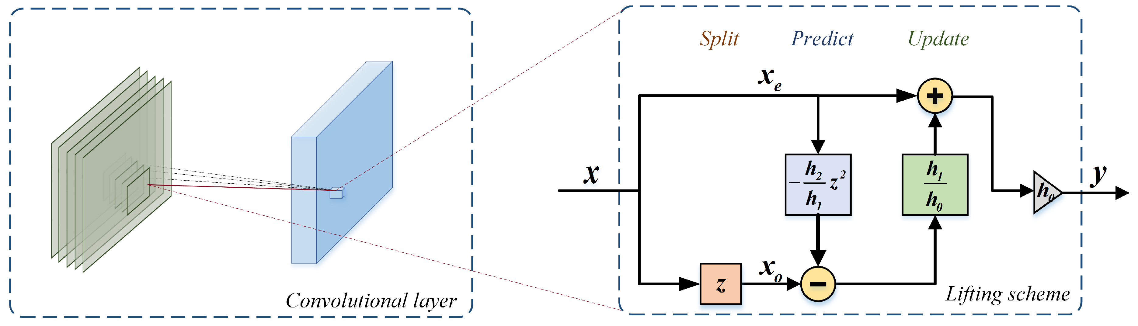
Given the matrix multiplication form in Equation (18), parameters of the lifting scheme, including the prediction and update operators and the scaling factor, are thus obtained. The 1 × 3 convolutional layer and its equivalent lifting scheme in one spatial plane are shown in Figure 2. In the 1 × 3 convolution, the convolution kernel moves across the input row by row in the horizontal direction to perform the sliding dot product. The lifting scheme can simultaneously process the entire input image within each of the steps listed in

Table 1. Steps of the lifting scheme equivalent to 1 × 3 convolutional layer.

Step	Illustration
split	${\mathit{x}}_{\mathit{e}}\left[i\right]=\mathit{x}\left[i\right]$, ${\mathit{x}}_{\mathit{o}}\left[i\right]=\mathit{x}[i+1]$
predict	${\mathit{x}}_{\mathit{o}}\left[i\right]={\mathit{x}}_{\mathit{o}}\left[i\right]+\frac{h_2}{h_1}\times {\mathit{x}}_{\mathit{e}}[i+2]$
update	${\mathit{x}}_{\mathit{e}}\left[i\right]={\mathit{x}}_{\mathit{e}}\left[i\right]+\frac{h_1}{h_0}\times {\mathit{x}}_{\mathit{o}}\left[i\right]$
scaling	$\mathit{y}\left[i\right]=h_0\times {\mathit{x}}_{\mathit{e}}\left[i\right]$

Note that notation $\mathit{x}\left[i\right]$ represents the ith column in image $\mathit{x}$.

.

As illustrated in Table 1, the input image passes through the three steps in the lifting scheme. In the split stage, the input is transformed into 2 branches, ${\mathit{x}}_{\mathit{e}}$ and ${\mathit{x}}_{\mathit{o}}$. Different from the lifting scheme in [14], we utilize a sliding window to obtain two branches instead of the lazy wavelet transform. Then, ${\mathit{x}}_{\mathit{o}}$ is predicted by ${\mathit{x}}_{\mathit{e}}$ with the predict operator $\frac{h_2}{h_1}{z}^2$, the outcome of which is used to update ${\mathit{x}}_{\mathit{e}}$. The final output is obtained by scaling the updated ${\mathit{x}}_{\mathit{e}}$ by the factor $h_0$.

2.2.2. The Lifting Scheme for the 2D Convolutional Layer

For a convolutional layer with 2D convolutional kernels, the lifting scheme can also be realized through the 1D lifting scheme. The 2D convolution operation is the sum of several 1D convolution operations. For instance, the output of the convolution operation between a $m\times n$ input image and a $3\times 3$ convolutional kernel has a size of $(m-2)\times (n-2)$. Then, the element on the i-th row, j-th column of the output matrix is obtained by

$$y(i,j)=\sum _{u=0}^2\sum _{v=0}^{2}x(i+u,j+v)·h(u,v)$$

(19)

which can be rewritten as

$$y(i,j)=\sum _{v=0}^{2}x(i,j+v)·h(0,v)+\sum _{v=0}^{2}x(i+1,j+v)·h(1,v)+\sum _{v=0}^{2}x(i+2,j+v)·h(2,v)$$

(20)

In other words, the 2D convolution operation is equivalent to the summation of three 1D convolution operations. As the relative lifting scheme of the 1D convolution has been worked out as the right side of Figure 2 shown, the 2D lifting scheme is simply the summation of the relative 1D lifting scheme.

Thus, any convolution kernels with random-valued parameters have equivalent lifting scheme implementation. As the prediction operator and update operator in the lifting scheme can be designed to fit other requirements, which correspond to a larger serving range than vanilla convolution, the lifting scheme is the superset of vanilla convolution. In other words, the vanilla convolutional layer is just a special case of the lifting scheme. To improve the feature extractor in the CNN, a more powerful lifting scheme structure can be designed by choosing other predict operators and update operators.

2.2.3. Backpropagation of the Lifting Scheme

In this part, we propose the backpropagation algorithm to train and update parameters in the lifting scheme. For simplicity, a new list of weights $\mathit{w}=[w_0,w_1,w_2]$ is used to represent the parameters in Figure 2 as

$$w_0=h_0,w_1=\frac{h_1}{h_0},w_2=\frac{h_2}{h_1}$$

(21)

Assume the backpropagation error from the next layer is L, then the gradient with respect to this layer’s output $\mathit{y}$ is obtained by

$$\Delta y(i,j)=\frac{\partial L}{\partial y(i,j)}$$

(22)

where $y(i,j)$ represents one pixel in the output feature map $\mathit{y}$.

According to the derivation rule, the gradients with respect to the weights are obtained as follows.

$$\begin{array}{cc}\hfill \Delta w_0& =\sum _i\sum _j\frac{\partial L}{\partial y(i,j)}\frac{\partial y(i,j)}{\partial w_0}=\Delta \mathit{y}\odot \mathit{x}+w_1·\Delta \mathit{y}\odot {\mathit{x}}^{\prime }+w_1·w_2·{\mathit{x}}^{\prime \prime }\hfill \end{array}$$

(23)

$$\begin{array}{cc}\hfill \Delta w_1& =\sum _i\sum _j\frac{\partial L}{\partial y(i,j)}\frac{\partial y(i,j)}{\partial w_1}=w_0·\Delta \mathit{y}\odot {\mathit{x}}^{\prime }+w_0·w_2·\Delta \mathit{y}\odot {\mathit{x}}^{\prime \prime }\hfill \end{array}$$

(24)

$$\begin{array}{cc}\hfill \Delta w_2& =\sum _i\sum _j\frac{\partial L}{\partial y(i,j)}\frac{\partial y(i,j)}{\partial w_2}=w_0·w_1·\Delta \mathit{y}\odot {\mathit{x}}^{\prime \prime }\hfill \end{array}$$

(25)

where ${\mathit{x}}^{\prime }$ is the map whose elements in each row are the one-position left shifting elements in the corresponding row of $\mathit{x}$. ${\mathit{x}}^{\prime \prime }$ is the map whose elements in each row are the two-position left shifting elements in the corresponding row of $\mathit{x}$. ${\mathit{x}}^{\prime }$ and ${\mathit{x}}^{\prime \prime }$ maintain the same size as $\mathit{x}$ with some boundary extension methods. The operator “⊙” represents the cross-correlation between two matrices. With these gradients, the weights can be updated by stochastic gradient descent.

2.3. Lifting Scheme-Based Deep Neural Network

In this section, the lifting scheme is introduced into the deep learning field, and a lifting scheme-based deep neural network (LSNet) method is proposed to enhance network performance. From Section 2.1 and Section 2.2, the lifting scheme can substitute the convolutional layer because it can perform convolution and utilize backpropagation to update parameters. Specifically, operators in the lifting scheme are flexible, which can be designed not only to make the lifting scheme equivalent to vanilla convolutional layers but also extended to meet other requirements. Thus, we develop the LSNet with nonlinear feature extractors utilizing the ability of nonlinear transformation of the lifting scheme.

2.3.1. Basic Block in LSNet

Nonlinearity enables neural networks to fit complex functions and thus strengthens their representation ability. As the lifting scheme is capable of constructing nonlinear wavelets, we introduce nonlinearity into the feature extraction module to build the LSNet. It is realized by designing nonlinear predict and update operators in the lifting scheme, which demonstrates the enormous potential of the lifting scheme to perform nonlinear transformation and enhance the nonlinear representation of the neural network.

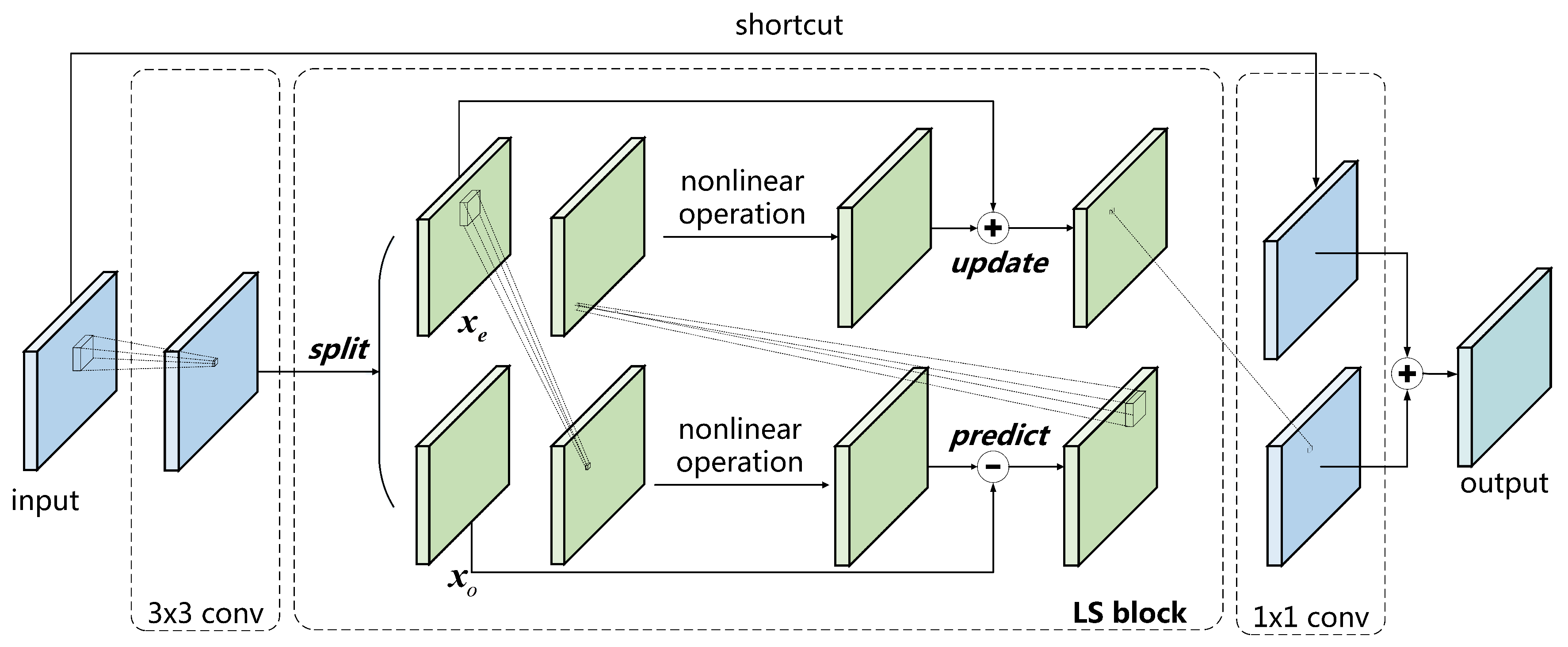
We construct the basic block in LSNet based on ResNet34 [35], as shown in Figure 3. The first layer in the basic block is a 3 × 3 convolutional layer, which is used to change the number of channels and downsampling. The middle layer is the LS block, mainly for feature extraction, with the same number of channels between the input and the output. The plug-and-play LS block is used to substitute the vanilla convolutional layer without any other alterations. In the LS block, the input is split into two parts, including ${\mathit{x}}_{\mathit{e}}$ and ${\mathit{x}}_{\mathit{o}}$. The nonlinear predict operator and update operator are constructed by a vanilla convolution kernel followed by a nonlinear function. ${\mathit{x}}_{\mathit{o}}$ is then predicted by ${\mathit{x}}_{\mathit{e}}$ to gain the detailed component, which is discarded after the update step. ${\mathit{x}}_{\mathit{e}}$ is updated by the detailed component, the outcome of which is the coarse component and used as the final output of the LS block. Finally, we add a 1 × 1 convolutional layer as the third layer to enhance channel-wise communication. Batch normalization and ReLU are followed by the first two layers for overfitting avoidance and activation, respectively. The identity of the input through a shortcut is added to the output of the third layer, followed by batch normalization. The addition outcome is again activated by ReLU, which is the final output of the basic block.

As both the 1D and 2D convolutional layers are widely used, we propose the 1D and 2D LS block, named the LS1D block and LS2D block, respectively. The specific processes of which are illustrated in

Table 2. Lifting scheme steps of LS1D block and LS2D block.

Step	LS1D Block	LS2D Block
split	${\mathit{x}}_{\mathit{e}}\left[i\right]=\mathit{x}\left[i\right]$, ${\mathit{x}}_{\mathit{o}}\left[i\right]=\mathit{x}[i+1]$	$x_e[i,j]=x[i,j]$, $x_o\left[i\right]=x[i+1,j+1]$
predict	${\mathit{x}}_{\mathit{o}}={\mathit{x}}_{\mathit{o}}-\mathcal{N}$ {Pconv1D$\left({\mathit{x}}_{\mathit{e}}\right)$}	${\mathit{x}}_{\mathit{o}}={\mathit{x}}_{\mathit{o}}-\mathcal{N}$ {Pconv2D$\left({\mathit{x}}_{\mathit{e}}\right)$}
update	${\mathit{x}}_{\mathit{e}}={\mathit{x}}_{\mathit{e}}+\mathcal{M}$ {Uconv1D$\left({\mathit{x}}_{\mathit{o}}\right)$}	${\mathit{x}}_{\mathit{e}}={\mathit{x}}_{\mathit{e}}+\mathcal{M}$ {Uconv2D$\left({\mathit{x}}_{\mathit{o}}\right)$}

Note that notation $\mathit{x}\left[i\right]$ represents the ith column in image $\mathit{x}$ while the notation $x[i,j]$ represents the ith row, jth column pixel in the image $\mathit{x}$.

.

Note that $\mathcal{N}\left\{·\right\}$ and $\mathcal{M}\left\{·\right\}$ denote the nonlinear transformation in the predict step and the update step, respectively. PconvnD$(·)$ and UconvnD$(·)$ represent the vanilla nD convolution operation in the predict and the update step, respectively. The operators $\mathcal{N}$ {PconvnD$(·)$} and $\mathcal{N}$ {UconvnD$(·)$} are the prediction and update operators, respectively, which are changeable to meet other requirements.

2.3.2. Network Architecture and Settings

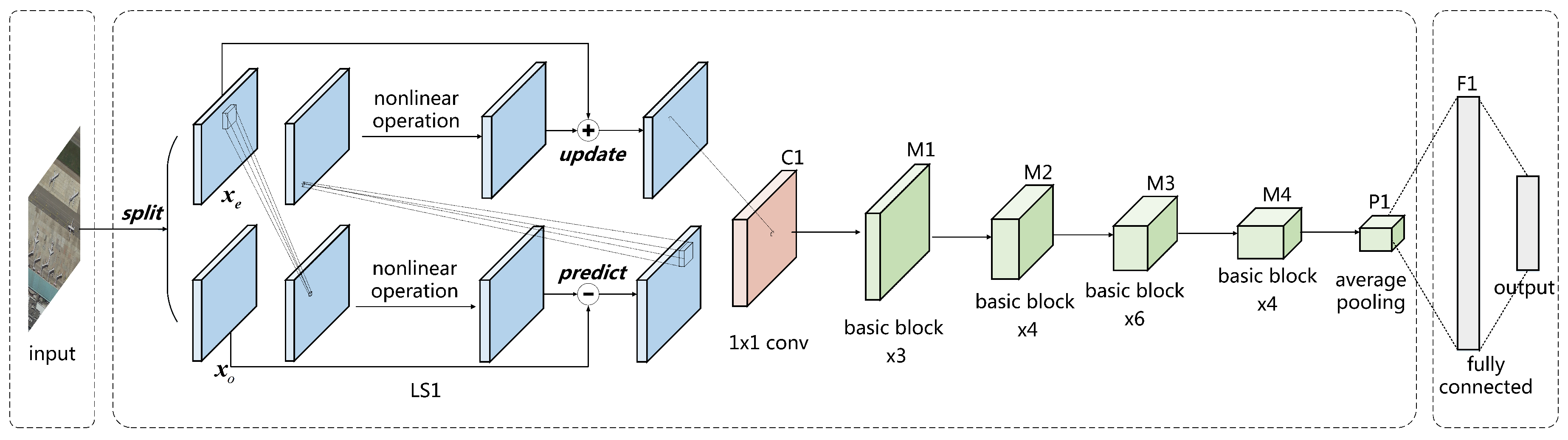
The network architecture of LSNet is shown in Figure 4. The input of LSNet passes through a single LS block and a 1 × 1 convolutional layer for initial feature extraction. The feature maps are then processed by stacked basic blocks to obtain low dimension image representation, which is followed by an average pooling for dimension reduction. Finally, the representation is unfolded as a 1D vector, and processed by a fully connected layer and a softmax function to obtain the output.

The modified ResNet34 is chosen as the baseline model to evaluate the performance of LSNet. Experiments are separately conducted for the 1D convolution and the 2D convolution, as both are widely used. The setups of each network are listed in

Table 3. Network architectures in contrast experiments.

Layer	ResNet-1d	LSNet-1d	ResNet-2d	LSNet-2d
LS1	$1\times 3,3$	LS1D block, 3	$1\times 3,3$	LS2D block, 3
C1	$1\times 1,64$
M1	$\left[\begin{array}{c}1\times 3,64\\ 1\times 3,64\\ 1\times 1,64\end{array}\right]\times 3$	$\left[\begin{array}{c}1\times 3,64\\ \mathrm{LS}1\mathrm{D} \mathrm{block},64\\ 1\times 1,64\end{array}\right]\times 3$	$\left[\begin{array}{c}3\times 3,64\\ 3\times 3,64\\ 1\times 1,64\end{array}\right]\times 3$	$\left[\begin{array}{c}3\times 3,64\\ \mathrm{LS}2\mathrm{D} \mathrm{block},64\\ 1\times 1,64\end{array}\right]\times 3$
M2	$\left[\begin{array}{c}1\times 3,128\\ 1\times 3,128\\ 1\times 1,128\end{array}\right]\times 4$	$\left[\begin{array}{c}1\times 3,128\\ \mathrm{LS}1\mathrm{D} \mathrm{block},128\\ 1\times 1,128\end{array}\right]\times 4$	$\left[\begin{array}{c}3\times 3,128\\ 3\times 3,128\\ 1\times 1,128\end{array}\right]\times 4$	$\left[\begin{array}{c}3\times 3,128\\ \mathrm{LS}2\mathrm{D} \mathrm{block},128\\ 1\times 1,128\end{array}\right]\times 4$
M3	$\left[\begin{array}{c}1\times 3,256\\ 1\times 3,256\\ 1\times 1,256\end{array}\right]\times 6$	$\left[\begin{array}{c}1\times 3,256\\ \mathrm{LS}1\mathrm{D} \mathrm{block},256\\ 1\times 1,256\end{array}\right]\times 6$	$\left[\begin{array}{c}3\times 3,256\\ 3\times 3,256\\ 1\times 1,256\end{array}\right]\times 6$	$\left[\begin{array}{c}3\times 3,256\\ \mathrm{LS}2\mathrm{D} \mathrm{block},256\\ 1\times 1,256\end{array}\right]\times 6$
M4	$\left[\begin{array}{c}1\times 3,512\\ 1\times 3,512\\ 1\times 1,512\end{array}\right]\times 3$	$\left[\begin{array}{c}1\times 3,512\\ \mathrm{LS}1\mathrm{D} \mathrm{block},512\\ 1\times 1,512\end{array}\right]\times 3$	$\left[\begin{array}{c}3\times 3,512\\ 3\times 3,512\\ 1\times 1,512\end{array}\right]\times 3$	$\left[\begin{array}{c}3\times 3,512\\ \mathrm{LS}2\mathrm{D} \mathrm{block},512\\ 1\times 1,512\end{array}\right]\times 3$
	average pooling, fully connected, Softmax

.

In Table 3, the size and the number of convolution kernels in vanilla convolutional layers are listed. For LSNet, the structure of the LS1D block and LS2D block are shown in Table 2, while the number represents the depth of the output. To demonstrate the effect of nonlinearity, we use five different nonlinear functions to construct different LS blocks to compare the performance, which are ReLU [3], leaky ReLU [4], ELU [5], and CELU and SELU [6].

In the experiment on the AID dataset, we use the stochastic gradient descent (SGD) as an optimizer, with a momentum of 0.9 and a weight decay of $5\times {10}^{-4}$. We train the training set for 100 epochs, setting the mini-batch size as 32. The learning rate is 0.01 initially, which decreases by 5 times every 25 epochs. For the CIFAR-100 dataset, all the settings are the same except that the mini-batch size is 128, and the initial learning rate is 0.1.

2.4. Materials

LSNet is firstly validated using the CIFAR-100 dataset [36], which is one of the most widely used datasets for deep learning reaches. Then, we conduct experiments on the AID dataset [37] to demonstrate the effectiveness of LSNet on the scene classification task.

CIFAR-100 dataset: This dataset contains 60,000 images, which are grouped into 100 classes. Each class contains 600 32 × 32 colored images, which are further divided into 500 training images and 100 testing images. The 100 classes in the CIFAR-100 dataset are grouped into 20 superclasses. In this dataset, a “fine” label indicates the class to which the image belongs, while a “coarse” label indicates the superclass to which the image belongs.

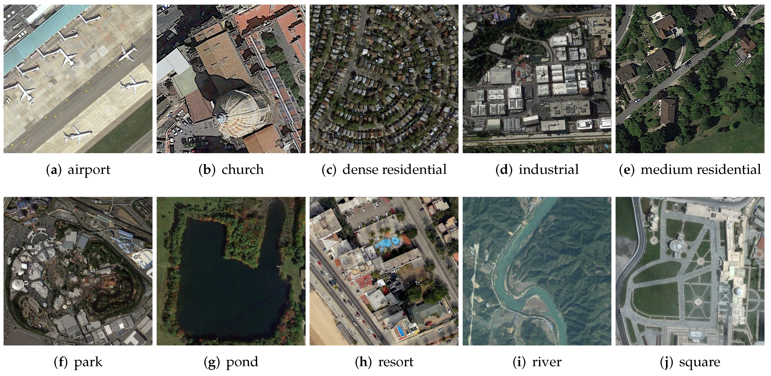
AID dataset: The AID dataset is a large-scale high-resolution remote sensing dataset proposed by Xia et al. [37] for aerial scene classification. With high intra-class diversity and low inter-class dissimilarity, the AID dataset is suitable as the benchmark for aerial scene classification models. Thirty classes are included, each with 220 up to 420 600 × 600 images. In our experiment, $80\%$ images of each class are chosen as the training data, while the rest $20\%$ are chosen as testing data. Each image is resized to 64 × 64. Some samples of the AID dataset are shown in Figure 5.

3. Results

In this section, LSNet is firstly validated using the CIFAR-100 dataset. Then, we put emphasis on evaluating LSNet on the AID dataset to demonstrate the effectiveness of LSNet on the scene classification task, the performance of which is compared with ResNet34 that utilizes vanilla convolution.

3.1. Results on the CIFAR-100 Dataset

The overall accuracy of the CIFAR-100 test set is used to evaluate the performance of LSNet, as shown in

Table 4. Performance of networks on the CIFAR-100 dataset in the 1D experiment.

Method	ResNet-1d	LSNet-1d
		ReLU	Leaky ReLU	ELU	CELU	SELU
Acc.(test)	73.00%	74.92%	74.71%	75.48%	74.98%	75.21%
Delta	−	$+1.92\%$	$+1.71\%$	$+\mathbf{2}.\mathbf{48}\%$	$+1.98\%$	$+2.21\%$

and

Table 5. Performance of networks on the CIFAR-100 dataset in the 2D experiment.

Method	ResNet-2d	LSNet-2d
		ReLU	Leaky ReLU	ELU	CELU	SELU
Acc.(test)	74.64%	75.52%	76.02%	75.76%	76.00%	74.21%
Delta	−	$+0.88\%$	$+\mathbf{1}.\mathbf{38}\%$	$+1.12\%$	$+1.36\%$	$-0.43\%$

. This metric is defined as the ratio of the number of correctly predicted samples to the number of samples in the whole test set, as shown in Equation (26).

$$p_c=\frac{{\sum }_{k=1}^n{P}_{kk}}{N}$$

(26)

where $P_{kk}$ represents the number of correctly classified samples in the kth class, while n and N are the number of categories and the number of samples in the whole test set, respectively. Compared with metrics that evaluate each category, $p_c$ is more intuitive and straightforward for comparing LSNet and ResNet on the CIFAR-100 dataset, which has 100 categories. The parameter Delta is the accuracy difference between LSNet-1d and ResNet-1d to demonstrate the performance of LSNet more intuitively.

In the 1D experiment, all of the LSNets that utilize different nonlinear functions in the LS1D block outperform the baseline network ResNet-1d by more than 1.5%. In between, LSNet-1d with ELU used in the LS1D block reaches the best test set accuracy, which is superior to the baseline network by 2.48%.

In the 2D experiment, LSNet-2d, whose LS2D block uses SELU as the nonlinear function, is slightly inferior to the baseline network ResNet-2d, while other LSNets all outperform the baseline network. In between, LSNet-2d with leaky ReLU used in the LS2D block performs best, which advantages over ResNet-2d by 1.38%.

The experimental results confirm the advantage of introducing nonlinearity into the feature extractor module. With different nonlinear functions, LSNets perform differently, which indicates the importance of choosing suitable nonlinear predict and update operators. For the 1D and 2D experiments, the most appropriate nonlinear functions are different, indicating that they are structure-dependent.

3.2. Results on the AID Dataset

For each evaluated network, the results of the AID test set’s overall accuracy are listed in

Table 6. Performance of networks on the AID dataset in the 1D experiment.

Method	ResNet-1d	LSNet-1d
		ReLU	Leaky ReLU	ELU	CELU	SELU
Acc.(test)	82.45%	84.40%	82.55%	83.90%	84.50%	83.50%
Delta	−	$+1.95\%$	$+0.10\%$	$+1.45\%$	$+\mathbf{2}.\mathbf{05}\%$	+1.05%

. For the 1D experiment, all LSNets with different nonlinear functions used in the LS1D block outperform the baseline ResNet-1d. Therefore, LSNet-1d with leaky ReLU performs similarly to ResNet-1d, while LSNet-1d with ELU reaches the highest test set overall accuracy, which is superior to ResNet-1d by 2.05%.

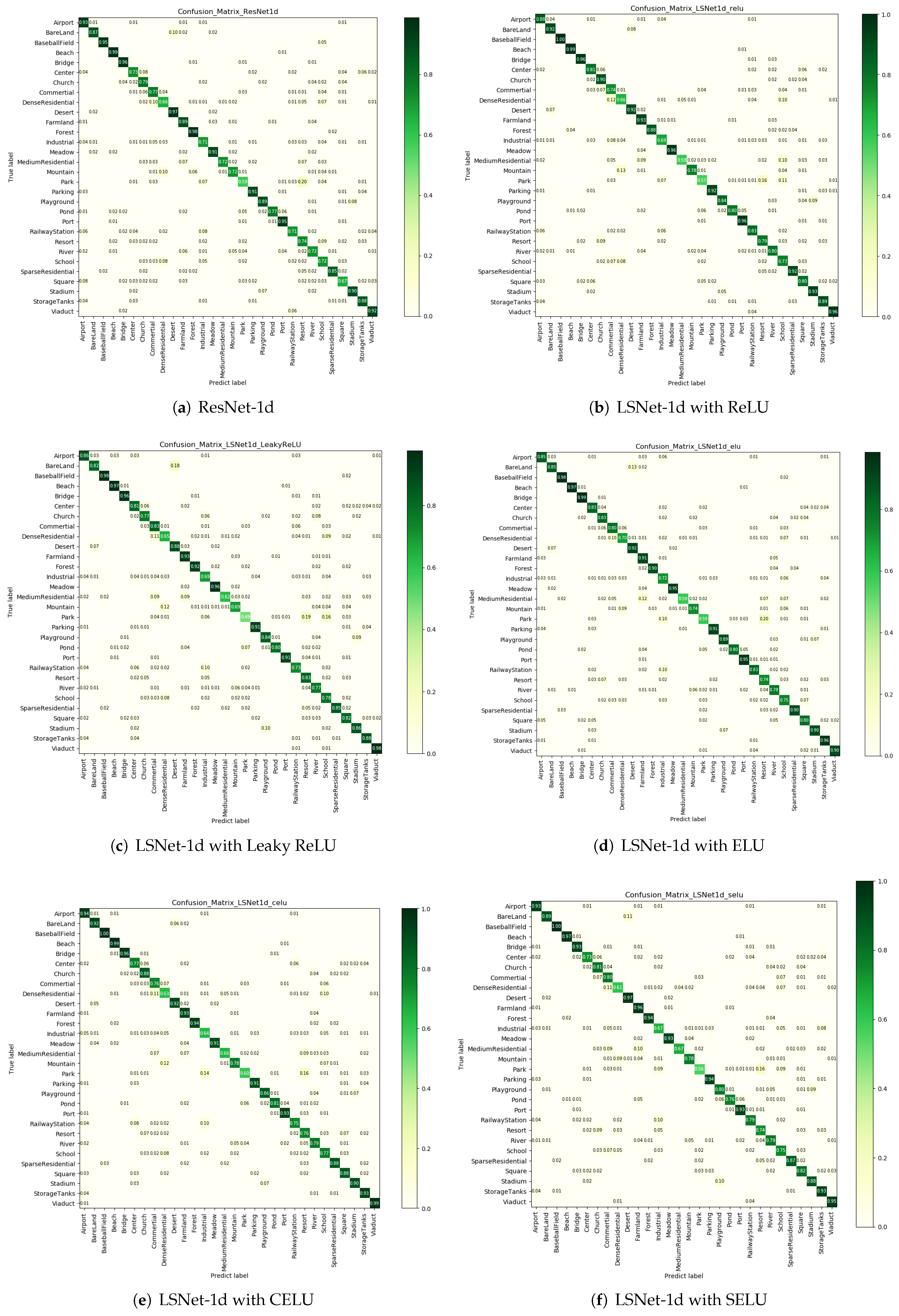
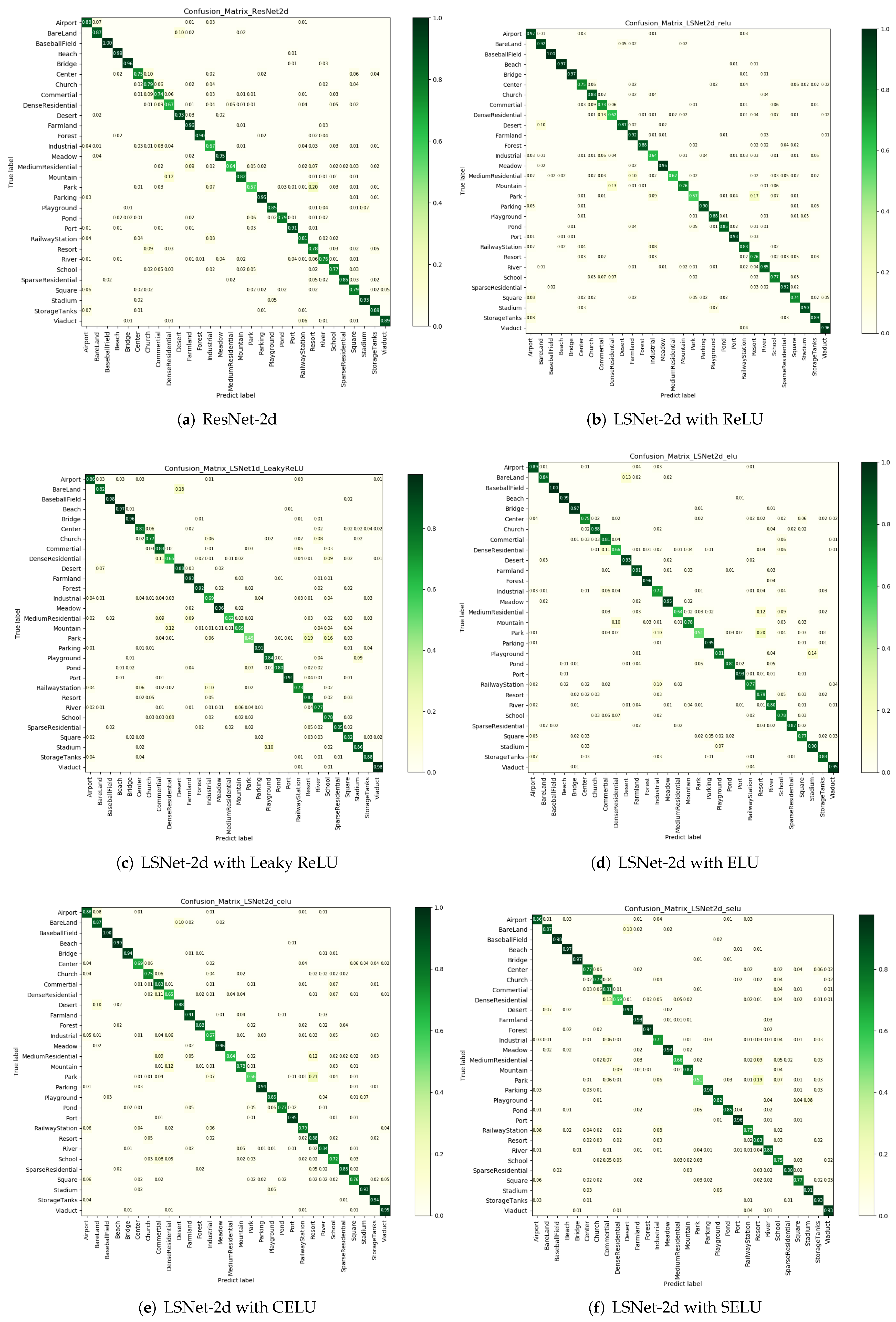
Confusion matrices for each evaluated network are shown in Figure 6. The probabilities whose values are more than 0.01 are displayed on the confusion matrices. Figure 6b–f are sparser than Figure 6a, which indicates smaller error rates and higher recalls. As Figure 6a shows, ResNet-1d performs well on some classes, such as baseball field, beach, bridge, desert, and forest, the recalls of which are higher than 95%. However, ResNet-1d confuses some classes with other classes. For instance, 20% of the images of the park class are mistaken as the resort class, while approximately 10% of the images of the mountain class are cast incorrectly into the dense residential class.

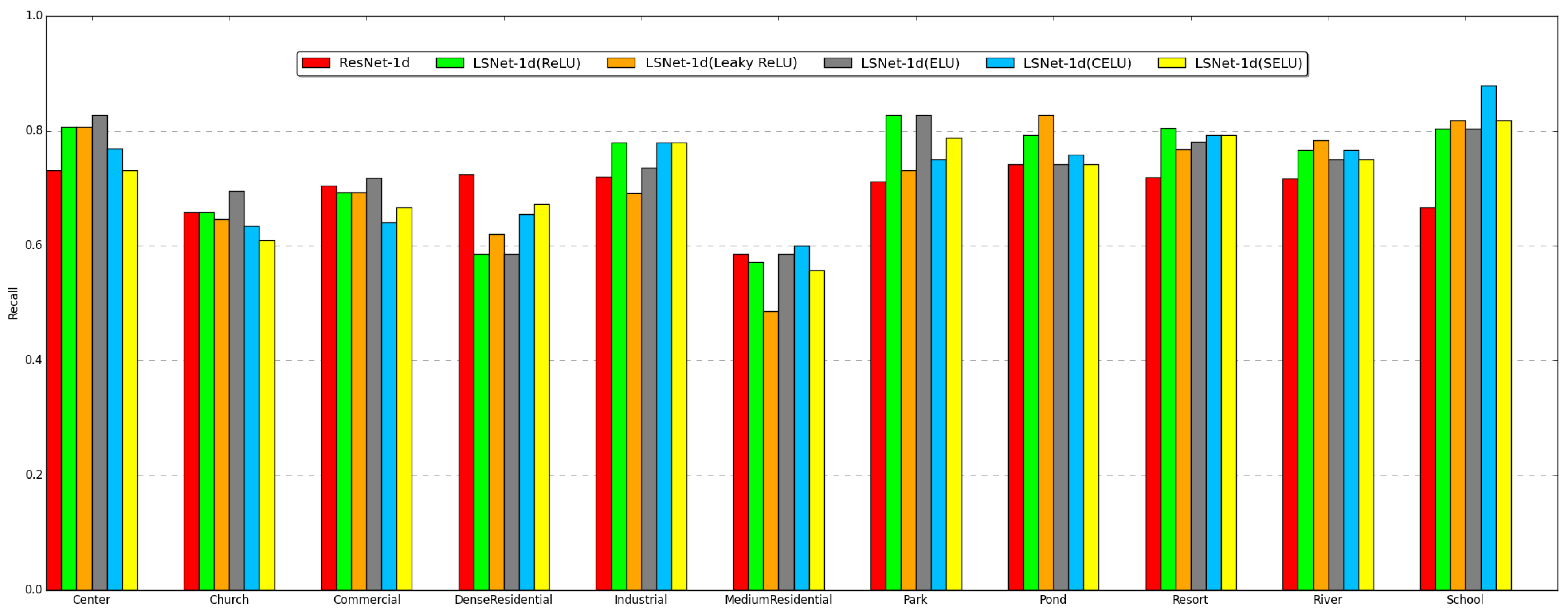
For further comparison between LSNet-1d and ResNet-1d, we select the classes whose recalls are below 75% in the ResNet-1d experiment and make further analysis. As shown in Figure 7, ResNet-1d surpasses all 1D LSNets on the medium residential class, but it is inferior to all 1D LSNets on five classes including railway station, resort, river, school, and square. All 1D LSNets are well ahead of ResNet-1d on the square class by more than 10%, which demonstrates that features extracted by nonlinear lifting scheme can better distinguish this class from all other classes.

In the 2D experiment, LSNets slightly enhance the performance compared with ResNet-2d, as shown in

Table 7. Performance of networks on the AID dataset in the 2D experiment.

Method	ResNet-2d	LSNet-2d
		ReLU	Leaky ReLU	ELU	CELU	SELU
Acc.(test)	83.30%	83.75%	83.20%	83.70%	83.55%	83.65%
Delta	−	$+\mathbf{0}.\mathbf{45}\%$	$-0.10\%$	$+0.40\%$	+0.25%	$+0.35\%$

. In between, LSNet-2d with ReLU used in the LS2D block achieves the highest test set accuracy, which is superior to ResNet-2d by 0.45%. Constructed by different nonlinear predict and update operators, the LS blocks construct different LSNets, which are distinguished in performance. This fact indicates the significance of seeking suitable nonlinear operators.

To explore the comparison between 2D LSNets and ResNet-2d, confusion matrices are drawn to displace the output probabilities whose values are more than 0.01, as shown in Figure 8. Recalls and error rates are displaced for each class. It can be determined that 2D LSNets perform better on some classes, such as the sparse residential class and the viaduct class, where all types of 2D LSNets are superior to ResNet-2d.

Furthermore, we select the classes whose recalls are below 80% in the ResNet-2d experiment and conduct further analysis. As shown in Figure 9, LSNets perform better on most of these classes. For instance, LSNet-2d with ReLU and LSNet-2d with ELU are superior to ResNet-2d by 8.4%, while LSNet-2d with CELU surpasses ResNet-2d by 7.8% on the commercial class. Moreover, all types of LSNets are better than ResNet-2d in river class. This fact indicates that the nonlinear lifting scheme provides an advantage in extracting the features to distinguish the river class from all other classes.

4. Discussion

Experimental results indicate that the proposed LSNet performs better than ResNet that utilizes the vanilla convolutional layer. An analysis of the improvement is as follows.

• LSNet can extract more discriminative features with the nonlinearity introduced by the lifting scheme. Corresponding to larger function space, features extracted from the nonlinear module are more distinguishable, which contains the information that cannot be represented by a linear convolutional layer. Therefore, LSNet reaches higher recall in a single class and perform better on the overall accuracy metric.
• The lifting scheme shown in Figure 2 is more suitable for hardware implementation with the advantages of in-place operation, acceleration, and auxiliary storage free, which can process the entire input image in parallel within each step. In the LSNet, the lifting scheme block performs prediction and update steps without transitional auxiliary storages. This characteristic of the LSNet is expected to provide the potential for easing the computational burden of high-resolution remote sensing imagery analysis and promoting applications on computationally limited hardware platforms.

In the future, we will introduce other nonlinear wavelets into neural networks, such as the morphology wavelet and the adaptive wavelet, to further enhance the nonlinear representation of neural networks. In addition, we will attempt to implant LSNet into some computationally limited platforms, such as FPGA, and compare its performance with existing methods.

5. Conclusions

CNN-based methods for scene classification are restricted by the computational challenge and limited ability to extract discriminative features. In this paper, the lifting scheme is introduced into deep learning and a lifting scheme-based deep neural network (LSNet) is proposed for remote sensing scene classification. The innovation of this approach lies in its capability to introduce nonlinearity into the feature extraction module to extend the feature space. The lifting scheme is an efficient algorithm for the wavelet transform to fit on the hardware platforms, which shows the potential of LSNet to ease the computational burden. Experiments on the AID datasets demonstrate that LSNet-1d and LSNet-2d are superior to ResNet-1d and ResNet-2d by 2.05% and 0.45%, respectively. The method proposed in this paper has room for further improvement, and we will introduce other nonlinear wavelets into neural networks and implant LSNet into some computationally limited platforms in the future.

References

- Hu, F.; Xia, G.S.; Hu, J.; Zhang, L. Transferring deep convolutional neural networks for the scene classification of high-resolution remote sensing imagery. Remote Sens. 2015, 7, 14680–14707. [Google Scholar] [CrossRef]
- Castelluccio, M.; Poggi, G.; Sansone, C.; Verdoliva, L. Land use classification in remote sensing images by convolutional neural networks. arXiv 2015, arXiv:1508.00092. [Google Scholar]
- Nair, V.; Hinton, G.E. Rectified linear units improve restricted boltzmann machines. In Proceedings of the 27th International Conference on Machine Learning (ICML-10), Haifa, Israel, 21–24 June 2010; pp. 807–814. [Google Scholar]
- Maas, A.L.; Hannun, A.Y.; Ng, A.Y. Rectifier nonlinearities improve neural network acoustic models. In Proceedings of the International Conference on Machine Learning (ICML), Atlanta, GA, USA, 16–21 June 2013; Volume 30, p. 3. [Google Scholar]
- Clevert, D.A.; Unterthiner, T.; Hochreiter, S. Fast and accurate deep network learning by exponential linear units (elus). arXiv 2015, arXiv:1511.07289. [Google Scholar]
- Klambauer, G.; Unterthiner, T.; Mayr, A.; Hochreiter, S. Self-normalizing neural networks. In Advances in Neural Information Processing Systems, Proceedings of the NIPS 2017, Long Beach, CA, USA, 4–9 December 2017; Neural Information Processing Systems Foundation: San Diego, CA, USA, 2017; pp. 971–980. [Google Scholar]
- Srivastava, N.; Hinton, G.; Krizhevsky, A.; Sutskever, I.; Salakhutdinov, R. Dropout: A simple way to prevent neural networks from overfitting. J. Mach. Learn. Res. 2014, 15, 1929–1958. [Google Scholar]
- Ioffe, S.; Szegedy, C. Batch normalization: Accelerating deep network training by reducing internal covariate shift. arXiv 2015, arXiv:1502.03167. [Google Scholar]
- Liu, B.D.; Meng, J.; Xie, W.Y.; Shao, S.; Li, Y.; Wang, Y. Weighted Spatial Pyramid Matching Collaborative Representation for Remote-Sensing-Image Scene Classification. Remote Sens. 2019, 11, 518. [Google Scholar] [CrossRef]
- Li, E.; Xia, J.; Du, P.; Lin, C.; Samat, A. Integrating Multilayer Features of Convolutional Neural Networks for Remote Sensing Scene Classification. IEEE Trans. Geosci. Remote Sens. 2017, 55, 5653–5665. [Google Scholar] [CrossRef]
- Chaib, S.; Liu, H.; Gu, Y.; Yao, H. Deep Feature Fusion for VHR Remote Sensing Scene Classification. IEEE Trans. Geosci. Remote Sens. 2017, 55, 4775–4784. [Google Scholar] [CrossRef]
- Flores, E.; Zortea, M.; Scharcanski, J. Dictionaries of deep features for land-use scene classification of very high spatial resolution images. Pattern Recognit. 2019, 89, 32–44. [Google Scholar] [CrossRef]
- Mallat, S.G. A theory for multiresolution signal decomposition: The wavelet representation. IEEE Trans. Pattern Anal. Mach. Intell. 1989, 11, 674–693. [Google Scholar] [CrossRef]
- Sweldens, W. Lifting scheme: A new philosophy in biorthogonal wavelet constructions. Proc. SPIE 1995, 2569, 68–80. [Google Scholar]
- Sweldens, W. The lifting scheme: A custom-design construction of biorthogonal wavelets. Appl. Comput. Harmon. Anal. 1996, 3, 186–200. [Google Scholar] [CrossRef]
- Sweldens, W. The lifting scheme: A construction of second generation wavelets. SIAM J. Math. Anal. 1998, 29, 511–546. [Google Scholar] [CrossRef]
- Sweldens, W. Wavelets and the lifting scheme: A 5 minute tour. ZAMM-Zeitschrift fur Angewandte Mathematik und Mechanik 1996, 76, 41–44. [Google Scholar]
- Sweldens, W.; Schröder, P. Building your own wavelets at home. In Wavelets in the Geosciences; Springer: Berlin, Germany, 2000; pp. 72–107. [Google Scholar]
- Daubechies, I.; Sweldens, W. Factoring wavelet transforms into lifting steps. J. Fourier Anal. Appl. 1998, 4, 247–269. [Google Scholar] [CrossRef]
- Skodras, A.; Christopoulos, C.; Ebrahimi, T. The Jpeg 2000 Still Image Compression Standard. IEEE Signal Process. Mag. 2001, 18, 36–58. [Google Scholar] [CrossRef]
- Lian, C.J.; Chen, K.F.; Chen, H.H.; Chen, L.G. Lifting based discrete wavelet transform architecture for JPEG2000. In Proceedings of the 2001 IEEE International Symposium on Circuits and Systems (ISCAS 2001), Sydney, NSW, Australia, 6–9 May 2001; (Cat. No. 01CH37196). IEEE: Piscataway, NJ, USA, 2001; Volume 2, pp. 445–448. [Google Scholar]
- Heijmans, H.J.; Goutsias, J. Nonlinear multiresolution signal decomposition schemes. II. Morphological wavelets. IEEE Trans. Image Process. 2000, 9, 1897–1913. [Google Scholar] [CrossRef]
- Claypoole, R.L.; Baraniuk, R.G.; Nowak, R.D. Adaptive wavelet transforms via lifting. In Proceedings of the 1998 IEEE International Conference on Acoustics, Speech and Signal Processing (ICASSP’98), Seattle, WA, USA, 12–15 May 1998; (Cat. No. 98CH36181). IEEE: Piscataway, NJ, USA, 1998; Volume 3, pp. 1513–1516. [Google Scholar]
- Piella, G.; Heijmans, H.J. Adaptive lifting schemes with perfect reconstruction. IEEE Trans. Signal Process. 2002, 50, 1620–1630. [Google Scholar] [CrossRef]
- Calderbank, A.; Daubechies, I.; Sweldens, W.; Yeo, B.L. Wavelet transforms that map integers to integers. Appl. Comput. Harmonic Analy. 1998, 5, 332–369. [Google Scholar] [CrossRef]
- Zheng, Y.; Wang, R.; Li, J. Nonlinear wavelets and bp neural networks adaptive lifting scheme. In Proceedings of the 2010 International Conference on Apperceiving Computing and Intelligence Analysis, Chengdu, China, 17–19 December 2010; IEEE: Piscataway, NJ, USA, 2010; pp. 316–319. [Google Scholar]
- Lin, M.; Chen, Q.; Yan, S. Network in network. arXiv 2013, arXiv:1312.4400. [Google Scholar]
- Szegedy, C.; Liu, W.; Jia, Y.; Sermanet, P.; Reed, S.; Anguelov, D.; Erhan, D.; Vanhoucke, V.; Rabinovich, A. Going deeper with convolutions. In Proceedings of the IEEE Conference on Computer Vision and Pattern Recognition, Boston, MA, USA, 7–12 June 2015; pp. 1–9. [Google Scholar]
- Howard, A.G.; Zhu, M.; Chen, B.; Kalenichenko, D.; Wang, W.; Weyand, T.; Andreetto, M.; Adam, H. Mobilenets: Efficient convolutional neural networks for mobile vision applications. arXiv 2017, arXiv:1704.04861. [Google Scholar]
- Szegedy, C.; Vanhoucke, V.; Ioffe, S.; Shlens, J.; Wojna, Z. Rethinking the inception architecture for computer vision. In Proceedings of the 2016 IEEE Conference on Computer Vision and Pattern Recognition (CVPR), Las Vegas, NV, USA, 27–30 June 2016; pp. 2818–2826. [Google Scholar]
- Rumelhart, D.E.; Hinton, G.E.; Williams, R.J. Learning representations by back-propagating errors. Cogn. Modeling 1988, 5, 1. [Google Scholar] [CrossRef]
- Oppenheim, A.V. Discrete-Time Signal Processing; Pearson Education India: Bengaluru, India, 1999. [Google Scholar]
- Jensen, J.R.; Lulla, K. Introductory digital image processing: A remote sensing perspective. Geocarto Int. 1987, 2, 65. [Google Scholar] [CrossRef]
- Romera, E.; Alvarez, J.M.; Bergasa, L.M.; Arroyo, R. Erfnet: Efficient residual factorized convnet for real-time semantic segmentation. IEEE Trans. Intell. Transp. Syst. 2017, 19, 263–272. [Google Scholar] [CrossRef]
- He, K.; Zhang, X.; Ren, S.; Sun, J. Deep residual learning for image recognition. In Proceedings of the IEEE Conference on Computer Vision and Pattern Recognition, Las Vegas, NV, USA, 27–30 June 2016; pp. 770–778. [Google Scholar]
- Krizhevsky, A.; Hinton, G. Learning Multiple Layers of Features from Tiny Images; Technical report; Citeseer: Princeton, NJ, USA, 2009. [Google Scholar]
- Xia, G.S.; Hu, J.; Hu, F.; Shi, B.; Bai, X.; Zhong, Y.; Zhang, L.; Lu, X. AID: A benchmark data set for performance evaluation of aerial scene classification. IEEE Trans. Geosci. Remote Sens. 2017, 55, 3965–3981. [Google Scholar] [CrossRef] [Green Version]
Figure 1.
Convolutional neural network (CNN) framework. CNN generally contains three modules, including feature extraction module, quantization module, and tricks module. These three modules are repeatedly stacked to build the deep structure, and finally, a classification module is applied for the specific classification task. The trick module is embedded in the other two modules, which is not displayed in this figure.
Figure 2.
Equivalence between the 1 × 3 convolution and the lifting scheme. The convolution kernel moves across the entire input image row by row to conduct the sliding dot product and generate the output feature maps. The lifting scheme can process the entire input image in parallel within each step. The lifting scheme implementation with three steps is equivalent to a vanilla 1 × 3 convolution in one plane.