An Efficient Encoding Voxel-Based Segmentation (EVBS) Algorithm Based on Fast Adjacent Voxel Search for Point Cloud Plane Segmentation

Abstract

Plane segmentation is a basic yet important process in light detection and ranging (LiDAR) point cloud processing. The traditional point cloud plane segmentation algorithm is typically affected by the number of point clouds and the noise data, which results in slow segmentation efficiency and poor segmentation effect. Hence, an efficient encoding voxel-based segmentation (EVBS) algorithm based on a fast adjacent voxel search is proposed in this study. First, a binary octree algorithm is proposed to construct the voxel as the segmentation object and code the voxel, which can compute voxel features quickly and accurately. Second, a voxel-based region growing algorithm is proposed to cluster the corresponding voxel to perform the initial point cloud segmentation, which can improve the rationality of seed selection. Finally, a refining point method is proposed to solve the problem of under-segmentation in unlabeled voxels by judging the relationship between the points and the segmented plane. Experimental results demonstrate that the proposed algorithm is better than the traditional algorithm in terms of computation time, extraction accuracy, and recall rate.

1. Introduction

With the development of three-dimensional (3D) laser scanning technology, it is simpler and more accurate to acquire point cloud data. A large number of 3D reconstruction applications have been developed in various fields using 3D laser scanning, such as cultural heritage protection, navigation and positioning, and urban planning [1,2,3]. Planar features are important in both indoor and outdoor 3D scenes. For large-scale 3D scene reconstructions, complex objects can be reconstructed better by the segmentation and recognition of planar shapes [4,5,6]. Traditional plane segmentation algorithms are limited by the large amount of point cloud data and the search method of neighbor points, which result in slow computation efficiency. Most segmentation criteria use only pairwise information between elements and are sensitive to missing points and structural incompleteness caused by occlusions [7]. Furthermore, the effectiveness and accuracy of a plane segmentation algorithm is affected by noise points and unevenly distributed points. According to the difference in segmentation objects, point cloud plane segmentation methods can be divided into two categories: point-based and voxel-based point cloud segmentation algorithms.

A point-based plane segmentation algorithm uses a single point as the object of plane segmentation and further classifies points of similar plane characteristics according to certain rules. Such algorithms can be classified into clustering-feature-based methods, model-fitting-based methods, and region-growing-based methods. Clustering-feature-based methods use the spatial coordinates, curvatures, and normal vectors of points to cluster spatial points by K-means, maximum likelihood, and fuzzy clustering [8,9,10,11]. The results of using clustering-feature-based methods are significantly affected by feature calculation and clustering method selection. Moreover, this method typically fails to cluster boundary points correctly. Model-fitting-based methods typically use planes, cylinders, spheres, and other geometric shapes to segment all or part of the point cloud data and classify points satisfying the fitting parameter model as the same group. The random sampling consistency (RANSAC) algorithm [12,13,14,15,16,17] is a typically used model-fitting-based method. This method can estimate plane parameters with high accuracy even when a large number of outliers exist. However, owing to the random selection of points to fit the geometric model using RANSAC, the algorithm demonstrated poor stability. The segmentation effect is greatly affected by the fitting distance $d$, and it is easy to produce over-segmentation and under-segmentation. Region-growing-based methods aggregate neighbor points of similar characteristics into clusters iteratively; it was first proposed by Besl and Jain [18]. In this method, seed selection and growing criteria are two main factors affecting the results. Rabbani et al. used the minimum residual of plane fitting as the criterion for seed selection [19], whereas Cai et al. computed variance of distances from initial seed k nearest points to the plane estimated by these points and the height difference between the certain point to the highest point in its cylinder-based neighborhood to select a real seed point, this method can exclude those low noise points as seed point [20]. For the growing criteria, normal vector consistency, surface smoothness, curvature, and a combination of various factors are typically selected. Rabbani et al. selected smoothness as the constraint of region growing to segment point clouds [19]. Tovari and Feifer selected the normal vector of a point cloud and the distance from neighbor points to the fitting plane as the criteria for region growing [21]. However, region-growing-based methods require obtaining neighbor points and computing the feature information of each point, which results in an inefficient computation. Furthermore, they are affected by noise points and normal consistency and can also easily produce over-segmentation and under-segmentation phenomenon.

Compared with point-based plane segmentation algorithms, a voxel-based plane segmentation algorithm uses voxels instead of scattered point clouds for plane segmentation, which builds grids to generate voxels based on the original point cloud and then uses voxel as objects for plane segmentation. Woo et al. introduced a new segmentation method that uses an octree-based 3D mesh to process a large number of disordered point cloud datasets [22]. The final 3D mesh was constructed by a refining process and iteratively subdividing voxels using the normal vectors of points. Because the normal vector of the voxel was the average value of the normal vectors of all points in the voxel, the computational efficiency of this algorithm was poor. In 2016, Su et al. proposed an octree-based segmentation and merging algorithm [23]. First, the input point cloud was divided into voxels until each voxel contains only coplanar points during segmentation. A new segmentation and merging framework based on graph theory and a series of connectivity were proposed to split and merge voxels. However, this method was primarily used in industrial scenarios, and its effect on plane segmentation has not been verified. Vo et al. combined an octree structure with a region growing algorithm to segment point cloud planes fast to accommodate 3D point clouds in urban environments [24]. But this method can’t find boundary voxels accurately, especially at the junction of two or more planes. Xu et al. proposed a point cloud segmentation strategy based on voxel structure and graph theory, where clustering was performed according to perceptual rules [7]. The algorithm enables a learning-free and completely automatic but parametric method for segmenting 3D point clouds. However, this method requires many parameters, and over-segmentation and under-segmentation are not considered in-plane segmentation. Lin et al. formalized supervoxel segmentation as a subset selection problem and then solved it using a heuristic algorithm [25]. This algorithm does not depend on the selection of seed points, and the extracted supervoxels can preserve the edges of the target object more effectively. However, this algorithm is only a segmentation method for point clouds and does not cluster supervoxels as a plane, thus rendering it inconvenient to use its result directly. In conclusion, voxel-based plane segmentation algorithms are complex and inefficient in voxel search and some shortcomings exist in voxel clustering, such as unreasonable seed selection, inadequate bases for selecting growing conditions, over-segmentation and under-segmentation, and unsatisfactory processing effects.

To improve the efficiency and quality of plane segmentation based on a large number of point cloud data, an efficient encoding voxel-based segmentation (EVBS) algorithm based on a fast adjacent voxel search is presented herein. Firstly, a highly efficient point cloud voxelization method is proposed to improve the efficiency of voxels and point cloud searching. It is the basis of fast and accurate point cloud plane segmentation. Secondly, by improving the selection of seed voxels and the determination of constraints in region growing algorithm, point cloud planes are segmented more accurately. Finally, to solve the problem of over-segmentation, the voxels with lower plane features are not labeled and clustered into any plane in the initial segmentation. Then for these unlabeled voxels, a method of refining points in unlabeled voxel by judging the relationship between the points and the segmented planes is proposed to solve the problem of under-segmentation which is just an easy implement.

2. Methods

The process of the EVBS algorithm is shown in Figure 1, which includes four main steps: (1) Using a highly efficient binary-coded octree to voxelize the point cloud, which can realize a fast voxel adjacency search; (2) estimating the features of each voxel, including the spatial position, normal vector, and residual value of the voxel; (3) clustering voxels using a region growing algorithm, in which the effects of residual value and number of points in voxels are considered while selecting a reasonable seed voxel; smoothness and continuity constraints are used as two main constraints for region growing; (4) refining point clouds in unlabeled voxels by judging the relationship between points and the segmented plane to improve the recall rate and accuracy of plane segmentation.

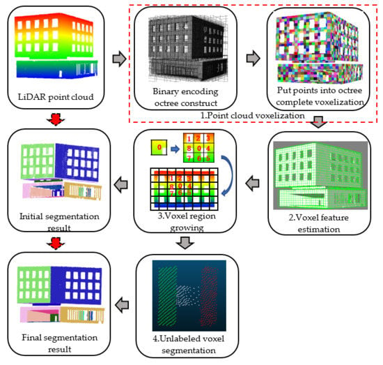
2.1. Point Cloud Voxelization

2.1.1. Voxelization Based on Binary Coding Octree

As with many unstructured spatial data sets, some spatial indexing techniques are used to support faster search and access to data. Octree and k–d trees are widely used in the field of point cloud processing to organize disorder point clouds. K–d tree is a binary search tree, which is very useful for interval and neighbor search of point. Octree is a kind of tree data structure used to describe three-dimensional space. Each node of an octree represents the volume element of a cube, and each node has eight child nodes. In order to improve the efficiency and stability of point cloud segmentation, voxel is used to instead of point as the object of plane segmentation, so it is necessary to use octree to complete the voxelization of the point cloud [26] (k–d tree cannot complete the voxelization of the point cloud). The region growing algorithm is used in this paper, which merges the voxels with adjacent relationship and similar plane features. Therefore, it is important to search the adjacent voxels with highly efficient.

For a traditional octree to search for adjacent voxels, the search radius must be set and the corresponding voxels are obtained by recursive search; additionally, the relationship between child and parent nodes is assessed, which is not efficient, or a table-based storage and location are used, which requires significant memory. Therefore, traditional methods are not suitable for searching adjacent voxels when the point cloud is large [27,28]. In this paper, a novel point cloud voxelization method based on binary coding octree is proposed to do a fast search of adjacent voxels. The voxelization method is shown in Figure 2, which is described as follows: (1) The level of an octree was calculated according to the bounding box of the point cloud data and the set leaf node size $d_I$. (2) Eight child nodes were divided from the parent node and coded according to the X, Y, and Z axes with 0 or 1, as shown in Figure 2a. The initial coding of eight child nodes was obtained by combining the coding of X, Y and Z axes. Figure 2b shows the coding value of the node when level = 1. Then adding the encoding of the parent node to the front of the initial encoding of the child node to form the final encoding of the child node. Figure 2c shows the coding value of part voxels when level = 2. (3) After the coding method was determined, the relationship between node coding and coordinates was established. We used the octree which level = 2 and $d_I$ = 1 m as an example: the binary code of a node is 111,011 as shown in Figure 2c, of which steps are shown as follows:

• Extract the code value related to X in the code, i.e., the value 1 of the first bit and the value 0 of the fourth bit, constitute the binary code is 10, and the decimal system is 2, then the voxel X coordinate is 2 $\times$ 1 = 2 m.
• Similarly, Y = 3 $\times$ 1 = 3 m and Z = 3 $\times$ 1 = 3 m.

Conversely, when we know the coordinates of a point $p$, we can convert it into binary code using Equation (1):

$$\begin{array}{l}{X}_b=binary(floor((p.x-O.x)/d_I)\\ Y_b=binary(floor((p.y-O.y)/d_I)\\ Z_b=binary(floor((p.z-O.z)/d_I)\end{array}$$

(1)

where, $X_b$, $Y_b$ and $Z_b$ are the coding of three coordinate values of $p$, $O$ is the origin point of octree. Then insert each bit of $X_b$, $Y_b$, $Z_b$ into the corresponding position, and the coding value of the voxel where this point located in can be obtained. Put all the points into the corresponding voxels to complete the voxelization of the point cloud. In order to speed up the extraction of encoded bits value, we use the bit operation instruction: parallel bits extract (PEXT) to extract the X, Y, Z three-dimensional spatial coordinates from the voxel encoding, and parallel bits deposit (PDEP) to insert the binary encoding bits of the three coordinate values of point cloud into different position and merge them into one encoding. This encoding method takes up little memory, and the speed of encoding and coordinate conversion is fast. It is suitable for the voxelization of point cloud with a large amount of data.

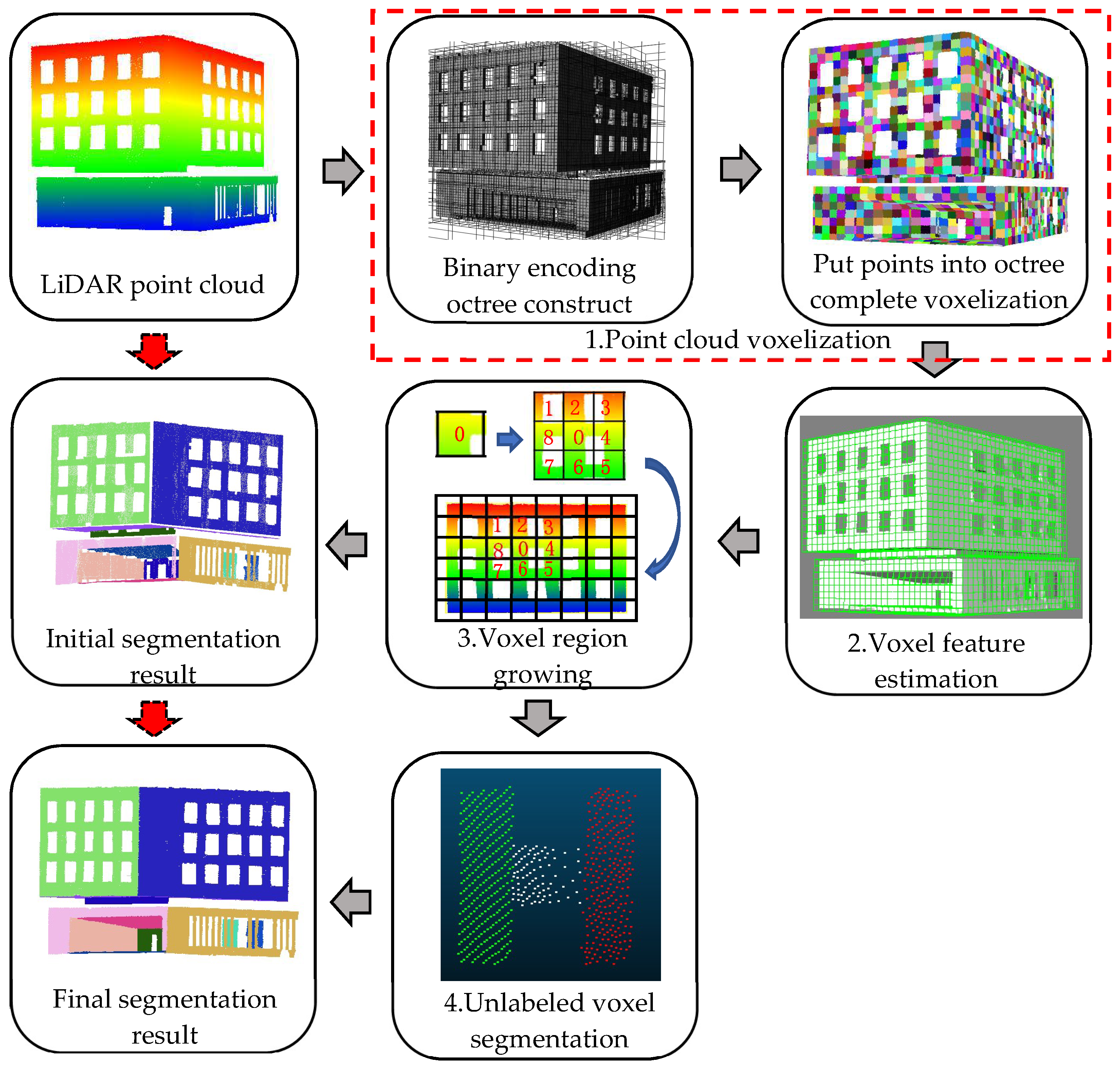
2.1.2. Searching Adjacent Voxel

Generally, point cloud data are disorganized. In this study, a 26-voxel adjacent topology structure is used to organize voxels and point clouds. When searching for adjacent voxels, the encoding of voxels on three coordinate axes X_ref, Y_ref, and Z_ref were obtained according to the bit operation instruction PEXT. Because the leaf node sizes of an octree are equal, the component coding of the leaf node on one coordinate axis differ by 1 or 0 between the leaf node and its adjacent leaf nodes, as shown in Figure 2c or Figure 3b. According to this feature, the encoding of the three coordinate axes of 26 adjacent voxels is calculated as follows:

$$\begin{array}{l}X=X_{ref}\pm 1(0)\\ Y=Y_{ref}\pm 1(0)\\ Z=Z_{ref}\pm 1(0)\end{array}$$

(2)

Finally, the binary encoding of adjacent voxels is calculated using the bit operation instruction PDEP according to the coding values of the three coordinate axes, and the corresponding voxels are obtained via binary encoding and the octree structure. This binary coding converts the general traversal comparison operation into a binary bit operation, which improves the search efficiency significantly and is the basis for the fast region growing of voxels. The results of voxel search are shown in Figure 3c; a red voxel represents the known coded voxel, whereas yellow and blue voxels represent adjacent voxels that have point clouds. Figure 3d shows the point cloud in the adjacent voxels.

2.2. Voxel Feature Estimation

Generally, the growing conditions of the point-based region growing algorithms were based on the features of points, which include the location, normal, and curvature of points. Similarly, a voxel region growing algorithm requires voxel features as growing conditions. Herein, three features of voxels are calculated: the spatial position, normal vector, and residual value of voxels, which are described as follows:

(1)

The spatial position of a voxel is expressed by the average coordinate values of all points in a voxel (centroid $O(\overline{x},\overline{y},\overline{z})$).

(2)

The normal vector of a voxel is calculated by principal component analysis (PCA). First, the covariance matrix is calculated by point set $P\left\{p_1,p_{2,}{p}_3\dots p_n\right\}$ in a voxel:

$$C=\frac{1}{n}{\displaystyle \sum _{i=1}^n(p_i-\overline{p}){(p_i-\overline{p})}^T}$$

(3)

where $\overline{p}=\frac{1}{n}{\displaystyle \sum _{i=1}^n{p}_i}$ is the centroid of a point cloud in a voxel and matrix $C$ is a symmetric positive definite matrix; matrix $C$ is decomposed into eigenvalues:

$$C=\left[\begin{array}{ccc}{e}_1& e_2& e_3\end{array}\right]\left[\begin{array}{ccc}{\lambda }_1& 0& 0\\ 0& {\lambda }_2& 0\\ 0& 0& {\lambda }_3\end{array}\right]\left[\begin{array}{c}{e}_1\\ e_2\\ e_3\end{array}\right]$$

(4)

where ${\lambda }_1, {\lambda }_2, {\lambda }_3$ are the three eigenvalues of matrix $C$ and ${\lambda }_1\ge {\lambda }_2\ge {\lambda }_3>0$; $e_1, e_2, e_3$ are the eigenvectors corresponding to the eigenvalues. The first eigenvector is the maximum variance direction of the point cloud data. The second eigenvector corresponds to the direction in which the data variance is the largest in the vertical direction of the first eigenvector, and so on. For point cloud plane estimation, the first two eigenvectors form the basis of the plane, the third eigenvector is orthogonal to the first two eigenvectors, and the normal of the fitting plane is defined [29]. In other words, the eigenvector corresponding to the minimum eigenvalue of the matrix is regarded as the normal vector of the point cloud data fitting plane in the voxel.

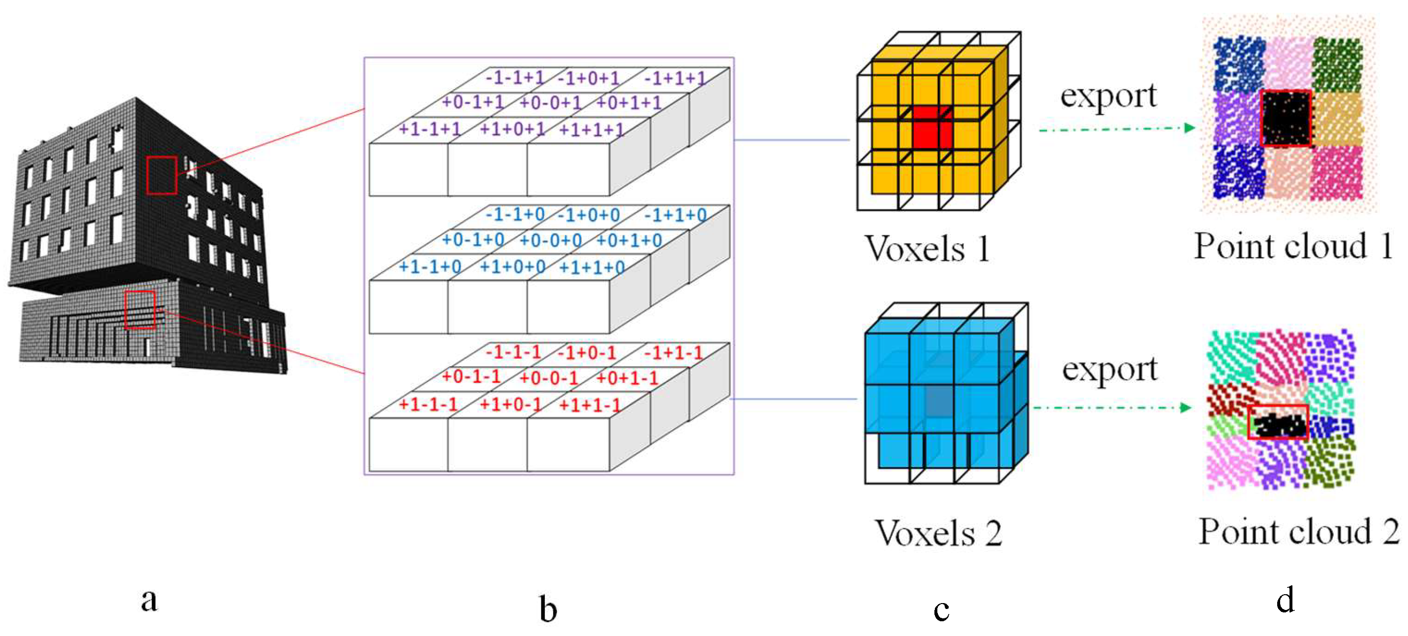
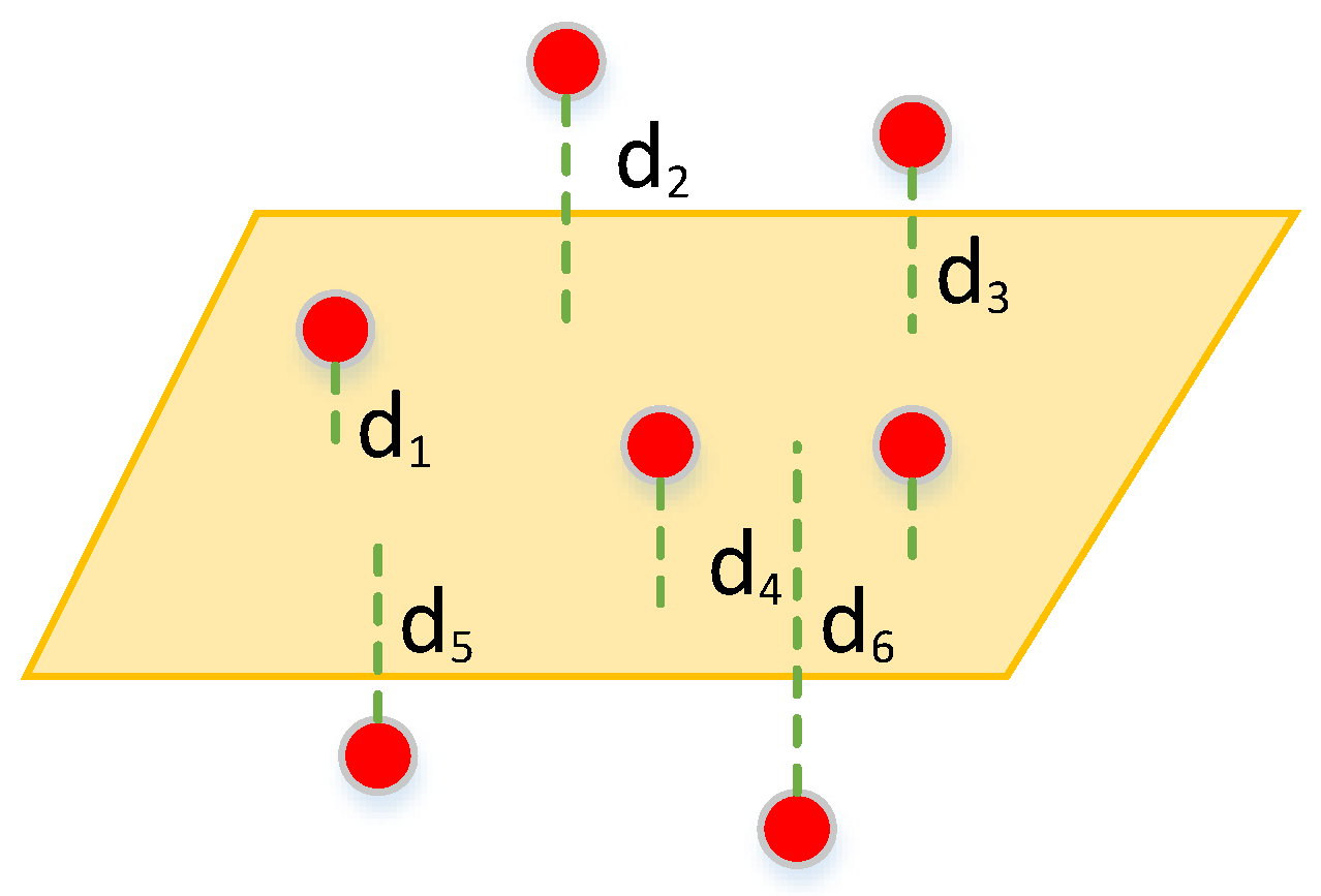
(3)

The residual in the plane fitting of point cloud data can be caused by noise points and the inconsistency between a point and a plane model. The equation for calculating the residual is as follows:

$$r=\sqrt{\frac{1}{k}{\displaystyle {\sum }_{i=1}^k{d}_i^2}}$$

(5)

where $d_i$ is the distance from the point to the fitting plane. For a single voxel, the residual value of a point cloud in a voxel indicates the degree of dispersion from points to the fitting plane, as shown in Figure 4. The smaller the residual value of the voxel, the higher is the flatness of a point cloud in a voxel.

2.3. Voxel-Based Region Growing

The region growing algorithm is an effective algorithm for point cloud segmentation. In the study by Rabbani et al. [19], points are regarded as growing objects and region growing is performed by calculating point features and smoothing constraints; thus, the segmentation of point clouds is completed. In this study, voxels are used to replace points as the object of plane segmentation. The two most important steps in a voxel-based region growing algorithm are the selection of seed voxel and the determination of growing constraints. Our methods are described as follows:

2.3.1. Selection of Seed Voxel

The traditional seed selection method of a voxel-based region growing algorithm is to sort voxels according to the residual value; subsequently, unclassified voxels are selected as the initial seed voxels for plane according to the order of voxel residual from small to large. It is generally believed that the smaller the residual value of voxel, the more likely the point cloud in voxel satisfies the plane features. But this method has not considered the effect of the number of points. If only three points exist in a voxel and a plane equation can be calculated, the residual of this voxel is 0. However, a voxel with fewer points is not suitable as a seed voxel because its feature is unstable. Therefore, in this study, the number of points of a voxel is used as a condition for selecting a seed voxel. Only when the number of points in a voxel is sufficient and the residual value is relatively small can this voxel satisfy the standard of a seed voxel. The normalized parameters of the number of points and voxel residuals are defined by weight functions:

$$w_i={\displaystyle \prod _{k\in \left[\begin{array}{cc}n& r\end{array}\right]}\exp \left(-\frac{{(D_k)}^2}{2{\lambda }_k^2}\right)}$$

(6)

where ${\lambda }_n,{\lambda }_r$ denote the bandwidths of the Gaussian kernel that controls the importance of point number and the residual value of a voxel, respectively. We set their values as 0.1. Furthermore, $D_k$ is the reflection of the point numbers $n$ and the residual value $r$ in voxels. In our method, the larger $n$ is and the smaller $r$ is, the more obviously the plane feature of this voxel is. In order to make the change of $n$ and $r$ have the same effect on the $w_i$, we set $D_n=1/n$ and $D_r=r_i$. Gaussian distribution is a weight distribution model. On the Gaussian distribution curve, the closer to the center 0, the larger the value. This just satisfies the characteristics that the closer the values of $1/n$ and $r$ are to 0, the more points are in the voxel and the more obvious the plane feature of the voxel is. This is why we use the Gaussian function to calculate the normalized parameter. To select the most reasonable seed voxel, the voxels are sorted according to the value of the normalized parameter $w$, and then the first unclassified voxel is selected as the initial seed voxel of one plane. Subsequently, the region growing of the voxels is performed according to the given constraints. Regarding the threshold value $w_{th}$ of the normalized parameters, when $w_i>w_{th}$ ($w_i$ is the normalized parameter value of the selected voxel), the growing procedure will be stopped. When one plane is growing, voxels that satisfy the given constraints and $w_i<w_{th}$ are selected as new seeds to continue growing this plane, until no suitable voxels are growing on this plane then continue to grow next plane. This implies that voxels whose normalized parameter is larger than $w_{th}$ will always be unlabeled in the initial segmentation.

2.3.2. Selection of Growing Conditions

The basic principle of voxel region growing is to iteratively estimate the similarity of all adjacent voxels and classify voxels whose similarity differences were within a certain range into one group. Points in voxels inherit the ID of the voxel cluster. The similarity of voxels was determined by the features of the voxels. Compared with the traditional region growing algorithm that only uses smoothness constraint, continuity constraint is proposed and added according to the definition of plane equation in this paper to cluster voxels which improved the accuracy of plane segmentation.

(1)

Smoothness constraint: Equation (7) expresses a plane equation in a 3D space. (A, B, C) is the normal of the plane. If points in two voxels are on the same plane, then the normal of the fitting planes of these two voxels should be approximately parallel. This is called the smoothness constraint.

$$Ax+By+Cz+D=0$$

(7)

Smoothness constraint is measured by comparing the angles between the normal vectors of two voxels. As shown in Figure 5a, two adjacent voxels A and B exist; their normal $v_A$ and $v_B$, respectively, have been computed in the feature estimation of voxels in Section 2.2. The angle between them is obtained by point multiplication, as shown in Equations (8) and (9):

$$\overrightarrow{v^A}·\overrightarrow{v^B}=v_x^A{v}_x^B+v_y^A{v}_y^B+v_z^A{v}_z^B=\Vert \overrightarrow{v^A}\Vert \Vert \overrightarrow{v^B}\Vert \cos \left({\theta }^{AB}\right)$$

(8)

$${\theta }^{AB}={\cos }^{-1}(v_x^A{v}_x^B+v_y^A{v}_y^B+v_z^A{v}_z^B)$$

(9)

If ${\theta }^{AB}\le {\theta }_{th}$, then these two voxels satisfy the smoothness constraints, and they are grouped into the same plane cluster; the point in these voxels are labeled by the cluster ID, as shown in Figure 5a; ${\theta }_{th}$ is the angle threshold. In Figure 5b, voxels A and B do not satisfy the smoothness constraint when ${\theta }^{AB}>{\theta }_{th}$.

(2)

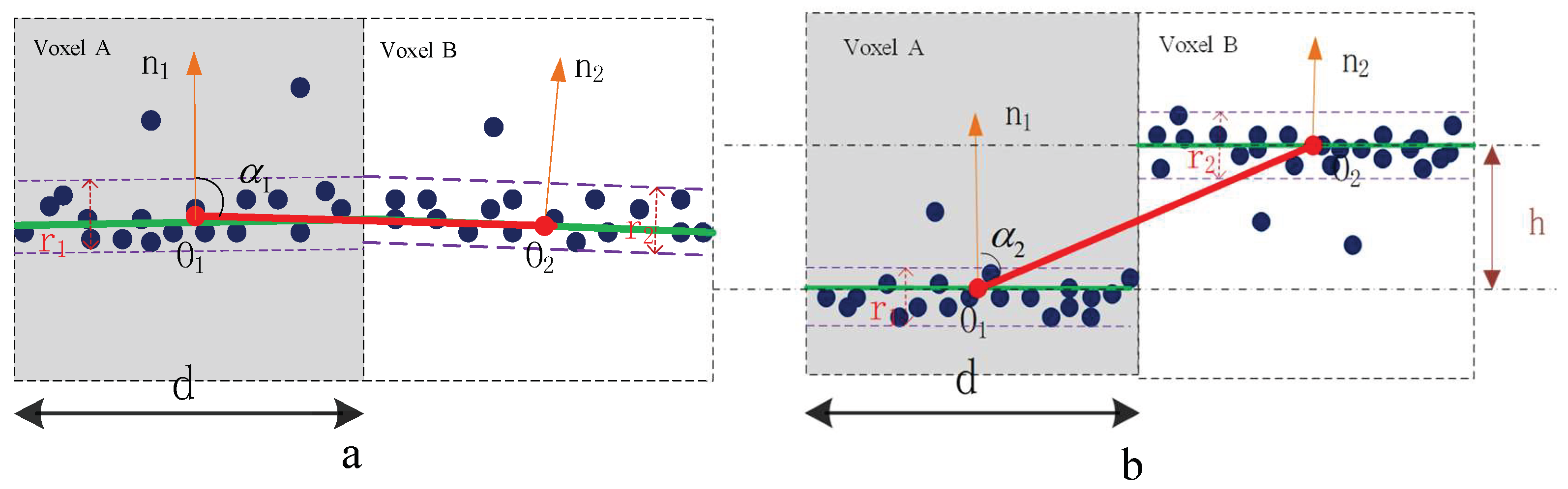
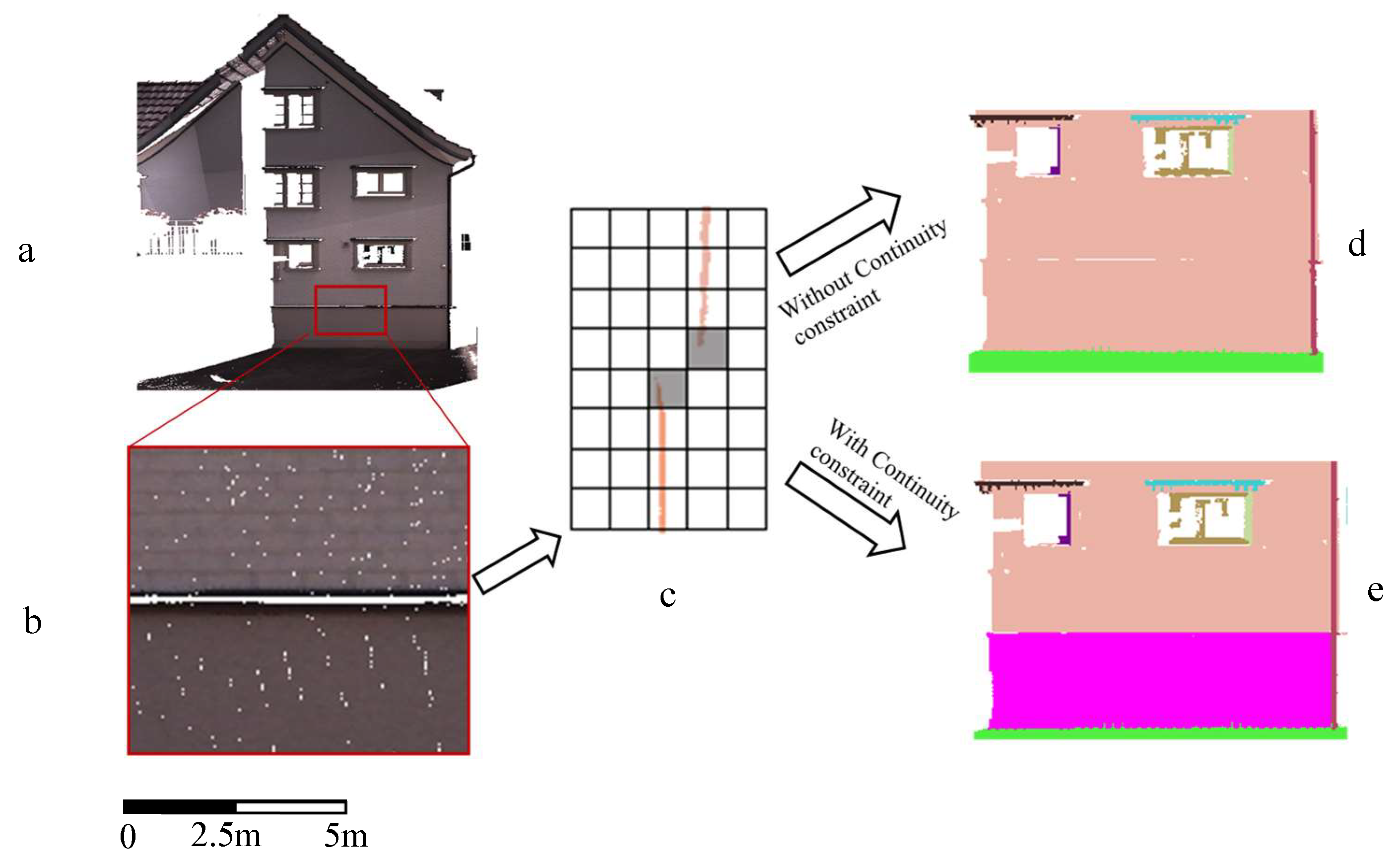
Continuity constraint: To judge whether points in two adjacent voxels belong to the same plane, it is insufficient to rely solely on the smoothness constraint. As shown in Figure 6b, the normal vectors of two adjacent voxels are parallel to each other, satisfying the smooth connection constraint; however, the point clouds of the two voxels do not belong to the same plane. Therefore, the parameter D in the plane equation should also satisfy the corresponding conditions to ensure that the points in the two voxels belong to the same plane. We call this constraint the continuity constraint. The continuity constraint of the voxels implies that if the points in two voxels belong to the same plane, then the two parts of the points are continuous, as shown in Figure 6a. To measure the continuity between two voxels, we compute the centroids $O_1$, $O_2$ of voxels A and B, respectively, and then connect the centroids of two voxels to obtain vector $\overrightarrow{O_1{O}_2}$. Before applying the continuity constraint, the smoothness constraint is first applied; in other words, the smoothness constraint is satisfied before the continuity constraint is applied. Therefore, the normal vectors of the two voxels are approximately parallel before the continuity constraint is applied. If $\overrightarrow{O_1{O}_2}·\overrightarrow{N_1}<{\phi }_{th}$ ($N_1$ is the normal of voxel A), the points in two voxels are considered to be continuous and cluster them into the same plane. If $\overrightarrow{O_1{O}_2}·\overrightarrow{N_1}>{\phi }_{th}$, then the point clouds in two voxels do not satisfy the continuity constraint. ${\phi }_{th}$ is the threshold. This can solve the problem of clustering the parallel planes which are close to each other into the same plane (shown in Section 4.3).

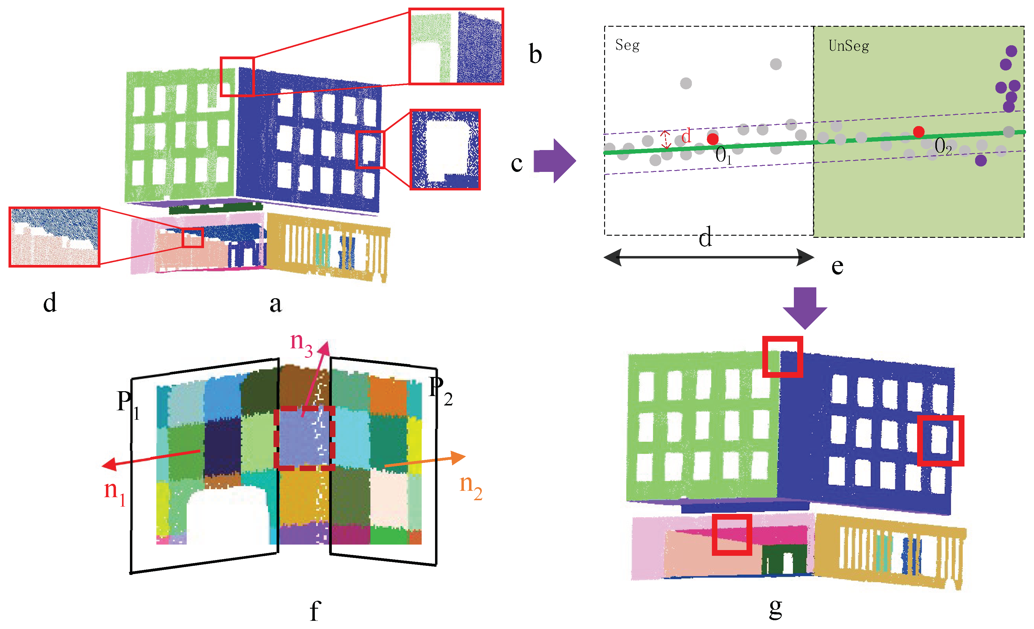
2.4. Unlabeled Voxel Segmentation

After the region growing segmentation of a voxel, points belonging to the same plane can be clustered into one group, and a set of point cloud planes can be obtained, as shown in Figure 7a. Although the point cloud planes are segmented correctly in the initial segmentation, there is a phenomenon of under-segmentation which caused by two main reasons: (1) the normal of voxel at the junction of two or more planes differs significantly from the normal of these planes, thus it is impossible for them to be clustered into any plane, as shown in Figure 7f; furthermore, because of the large residual value, they cannot be selected as a seed to grow a new plane, as shown in Figure 7b,d. (2) Some voxels are not clustered because of incorrect normal vector calculations owing to noise points, as shown in Figure 7c. To address under-segmentation, this paper allocates the points in unsegmented voxels correctly by judging the relationship between the plane of adjacent voxels that have been segmented from unsegmented voxels and the points in unsegmented voxels. First, we place the unsegmented voxels into a set $U$ and then traverse each unsegmented voxel $v_j$ in $U$ and find its adjacent voxel set $B$. Next, we record the index $m$ of the plane in which voxel $v_b$ is located, and $v_b\in B$. Subsequently, we calculate the distance from each point $p_i$ in $v_j$ to these planes, as shown in Equation (10).

$$\begin{array}{l}{d}_{\min }=\min \left\{\underset{m=0}{\overset{n}{dist}}\left(p_i,r_m\right)\right\}\\ \forall p_i\left(x_{{}_i},y_i,z_i\right)\in v_j,r_m\in R\end{array}$$

(10)

The distance $d_{\min }$ between a point and the nearest plane of its adjacent voxels, and the index $m_d$ of the nearest plane are calculated using the equation above. If $d_{\min }<d_{thd}$, then this point belongs to this nearest plane and is placed into the plane $R_{m_d}$; otherwise, this point is considered as noise data and will not be segmented, as shown in Figure 7e.

$$\{\begin{array}{c}{p}_i\in R_{m_d},if{d}_{\min }<d_{thd}\hfill \\ p_i\in \varnothing ,otherwise\hfill \end{array}$$

(11)

After the segmentation of unlabeled voxels, the integrality of the point cloud in building facades improved significantly, as shown in Figure 7g. The segmentation of unlabeled voxels proposed herein is easy to implement and efficient. It can effectively solve the problem of under-segmentation. The pseudocode is as follows:

Algorithm 1: Unlabeled voxel segmentation.

Data: Octree $O$, coarse segmentation plane set $R$, distance threshold $d_{thd}$.

Result: Place the points in the unsegmented voxels into the correct plane

initialization: Place the unsegmented voxel in octree $O$ into $U$

begin:

for each $v_j\in U$ do     find adjoin voxels B of $v_j$     for each $p_i\in v_j$ do      for each $v_k\in B$       compute d between $p_i$ to $r_m$      find $d_{\min }$ and its $m_d$      if $d_{\min }$ < $d_{\min }$ then       insert $p_i$ into $R_{m_d}$

3. Experiments and Analysis

To test the efficiency and robustness of the proposed EVBS algorithm, it is compared with two traditional point-based plane segmentation algorithms: region growing algorithm (SCRG) using the smoothing constraint proposed in [19], and efficient RANSAC algorithm (ER) [17]. Furthermore, a voxel- and graph-based point cloud segmentation algorithm (VGS) is selected for comparison to validate the EVBS algorithm [7]. Two different sources of point data are selected as experimental data, which are acquired using a terrestrial laser scanner and a mobile laser scanner. To evaluate the automatic segmentation algorithm, two groups of point cloud data are segmented manually as the ground truth [30,31]. Then, the results of automatic segmentation were compared with those of manual segmentation to evaluate the advantages and disadvantages of the segmentation algorithm. According to the ground truth plane $s_i$, we obtained its corresponding plane $s_i^{\prime }$ that was segmented by algorithms. Subsequently, we calculated the precision, recall, and comprehensive evaluation F1 to evaluate the EVBS algorithm, as follows:

$$precision=\frac{\left|TP\right|}{\left|TP\right|+\left|FP\right|}$$

(12)

$$recall=\frac{\left|TP\right|}{\left|TP\right|+\left|FN\right|}$$

(13)

$$F1=2\times \frac{precision\times recall}{precision+recall}$$

(14)

(1) True positive (TP): the number of $p_t$, where $p_t\in (s_i\cap s_i^{\prime })$, (2) false positive (FP): the number of $p_f$, where $p_f\in s_i^{\prime },p_f\notin s_i$, and (3) false negative (FN): the number of $p_n$, where $p_n\notin s_i^{\prime },p_n\in s_i$.

The EVBS involves five parameters: voxel resolution $d_I$, normal vector angle threshold ${\theta }_{th}$, normalized parameter threshold $w_{th}$, continuity threshold ${\phi }_{th}$, and distance from a point to a plane in the refining process $d_{\min }$. The most important parameters are $d_I$ and $w_{th}$. Voxel size directly affects the performance and results of the algorithm. Therefore, it was necessary to select the appropriate voxel size such that the algorithm performs correctly and efficiently. We used the method of Vo et al. [24], who referred to Filin and Feifer [32], to determine the voxel size according to the point cloud density and the parameters of the fitting plane, as shown in Equation (15).

$$m_{\alpha }=\pm m_0\cdot \frac{12}{k\cdot s}$$

(15)

where $m_{\alpha }$ is the accuracy of the fitting plane slope; $m_0$ is the accuracy of the laser range measurement; $k_{}$ represents the number of points in the neighborhood; $s$ is the reciprocal of the point cloud density. The voxel size is determined as $d_I\ge \sqrt{k}\cdot s$. The normalized threshold $w_{th}$ controls the voxel selection of seeds in this algorithm. The setting of $w_{th}$ is closely related to the execution time of the algorithm. The larger the $w_{th}$, the more voxels become seed voxels, and the more planes appear; consequently, the execution time will increase, $w_{th}$ is typically set according to the experience value, which is set to 0.05 in this study. ${\theta }_{th}$ is the angle between the fitting planes of the point clouds in the two voxels, which is commonly used in the point cloud plane segmentation algorithm. Generally, its value is relatively fixed and easy to understand. In this paper, it is set to 25.8°. Similarly, ${\phi }_{th}$ is the embodiment of D in the fitting plane equation of the point cloud of two voxels, and its setting is relatively fixed in this paper (0.15). The last threshold $d_{\min }$ is set according to the already set threshold $d_{\min }=0.5\cdot d_I$. In conclusion, only $d_I$ and $w_{th}$ are sensitive to data in this paper, while the other three thresholds are usually fixed.

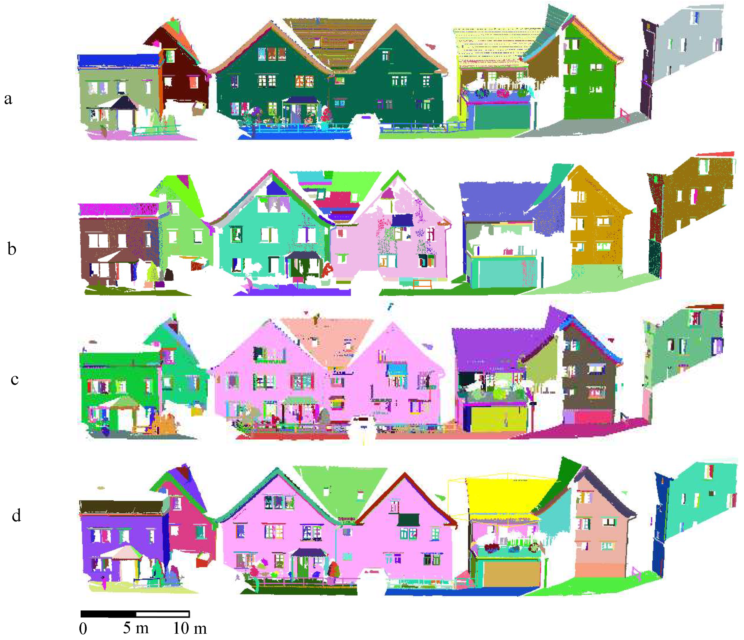
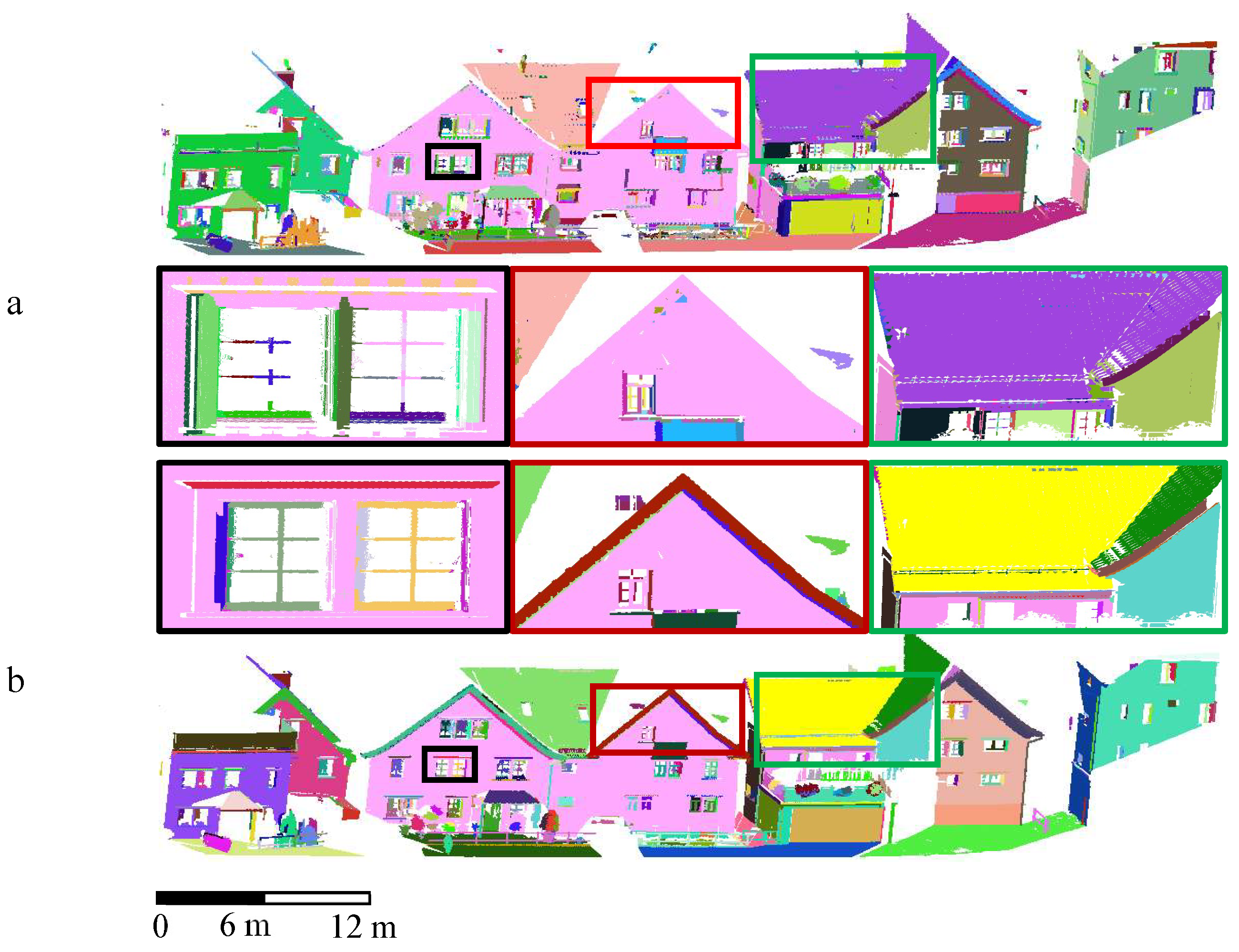
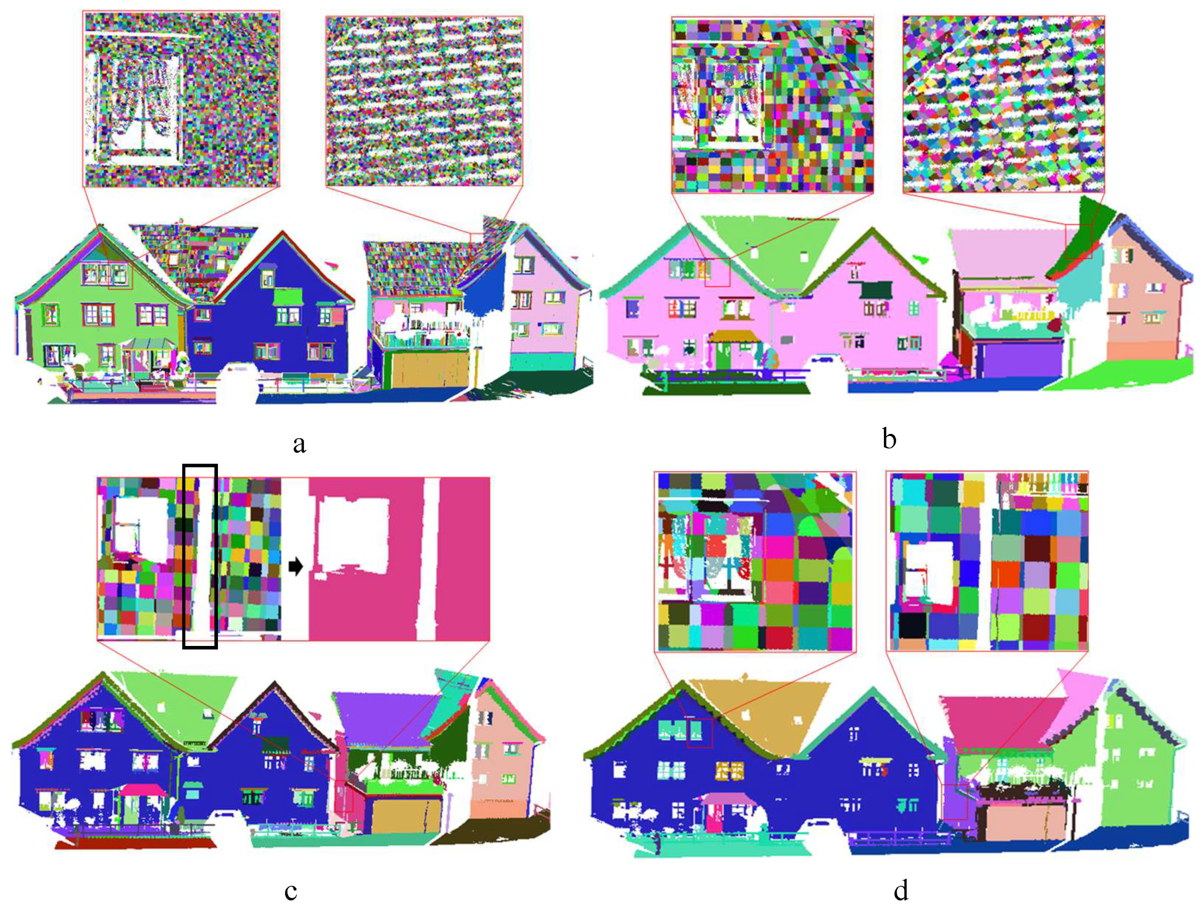
3.1. Results of Terrestrial Laser Scanner Data

The terrestrial light detection and ranging (LiDAR) data that we selected is the point cloud data of an urban scene. This data is part of sg27_10 of the large-scale point cloud data classification benchmark dataset [33] published by the Zurich Federal Institute of Technology (ETH Zurich) in 2016. It contains 28,112,328 3D points. This group of point cloud contains objects such as ground, walls, roofs, windows, and railings, as shown in Figure 8a. The ground truth data obtained by manual segmentation is shown in Figure 8b.

Table 1. Parameter settings for experiment using terrestrial laser scanner data.

	${\mathit{d}}_{\mathit{I}}\left(\mathbf{m}\right)$	${\mathit{w}}_{\mathit{t}\mathit{h}}\left(\mathbf{m}\right)$	${\mathit{\theta }}_{\mathit{t}\mathit{h}}\left(\mathbf{degree}\right)$	${\mathit{d}}_{\mathbf{min}}\left(\mathbf{m}\right)$
ER	0.034	-	25.8	0.034
SCRG	-	0.05	25.8
VGS	0.1	-	-	-
EVBS	0.1	0.05	25.8	0.05

shows the parameters of four methods for experiment using terrestrial laser scanner data.

The experimental results are shown in Figure 9. (1) Compared with point-based algorithms: because both the ER and SCRG must obtain the neighbor points of every point and the feature of this point is calculated according to the neighbor points, it is sensitive to noise. In addition, the normal of the point computed by neighbor points at the intersection of multiple planes are different from those of each plane; therefore, over-segmentation and under-segmentation will occur, as shown in Figure 9a,b. Our algorithm uses voxels to replace points as the object to segment. It is less affected by noise points and the features are more stable. Furthermore, by setting a smaller normalized parameter threshold, voxels at the junction of multiple planes are not labeled in the initial segmentation. The relationship between each point in the unlabeled voxels and the segmented plane is analyzed during refinement segmentation; subsequently, the points in the unlabeled voxels are segmented correctly, thus reducing over-segmentation and under-segmentation significantly, as shown in Figure 9d. As shown in

Table 2. Plane segmentation evaluation results of experiments using terrestrial laser scanner data.

	Precision	Recall	F1	Time (s)
ER	0.78	0.70	0.73	329.6
SCRG	0.51	0.53	0.52	749.3
VGS	0.80	0.62	0.70	77.3
EVBS	0.85	0.85	0.85	7.8

: the segmentation precision and recall rate of this algorithm are both 0.85, which are higher than 0.78 and 0.70 of the ER algorithm. Compared with the 0.51 and 0.53 of the SCRG algorithm, these two metrics increased by 66% and 60%, respectively. (2) Compared with the VGS algorithm: because the VGS algorithm uses a graph-based segmentation method, many parameters must be set, thus resulting in ambiguous plane clustering conditions that are not conducive to the segmentation of plane point clouds. Our algorithm uses the region growing method to cluster voxels; the best seed voxel was selected according to the point number and residuals in the voxel such that the best planes are clustered. Additionally, we used the equation of the plane to select growing conditions that more suitable for plane segmentation. These factors render the effect of our algorithm more detailed and smoother than that of the VGS algorithm, as shown in Figure 9c,d. For example, our algorithm can extract eaves successfully and extract windows more continuously, as shown in Figure 10a; however, the VGS algorithm exhibits errors in extracting roofs and cannot divide them into two planes, as shown in Figure 10b. From the segmentation results in Table 2, the segmentation precision of the EVBS is 0.85, which is greater than 0.80 of the VGS, and the comprehensive metrics F1 of this algorithm is 0.85, which is higher than 0.70 of the VGS.

In the segmentation of large-scale point clouds, efficiency is an important index to evaluate the performance of an algorithm. Compared with the traditional point-based segmentation algorithm, three factors contribute to the efficiency of our algorithm: (1) our method does not require the normal and characteristics of each point to be calculated, (2) voxels are used as growing objects, thus reducing the clustering time of a plane point cloud, and (3) reasonable selection of seed voxels prevents the generation of wrong planes and reduces the time of voxel clustering. As shown in Table 2, the EVBS only required 7.8 s to process the data, whereas the ER algorithm required 329.6 s and the SCRG algorithm required 749.3 s. The efficiency of EVBS is significantly improved. Compared with the voxel-based segmentation algorithm VGS, our algorithm uses a binary coding method to encode voxels, and adjacent voxels can be obtained quickly according to the voxel encode while the VGS searches adjacent voxels by setting the search radius, which results in poor search efficiency. Consequently, our algorithm is more advantageous than the VGS in processing terrestrial laser scanner data, as the time spent for processing is approximately 1/10 that of the VGS, as shown in Table 2.

To study the effect of different-size data on the efficiency of the segmentation algorithm, the original data of terrestrial laser scanner data are sampled according to different densities, and point cloud data by down-sampling are separately segmented by the ER, SCRG, VGS, and EVBS herein. The statistical graph of the execution time of four algorithms is shown in Figure 11. As shown, the execution times of the other three algorithms increase significantly with the number of point cloud data. But our algorithm was less affected by the increasing number of point clouds and keeps a high segmentation efficiency. It proves that our algorithm has more advantages in processing large-scale point cloud data.

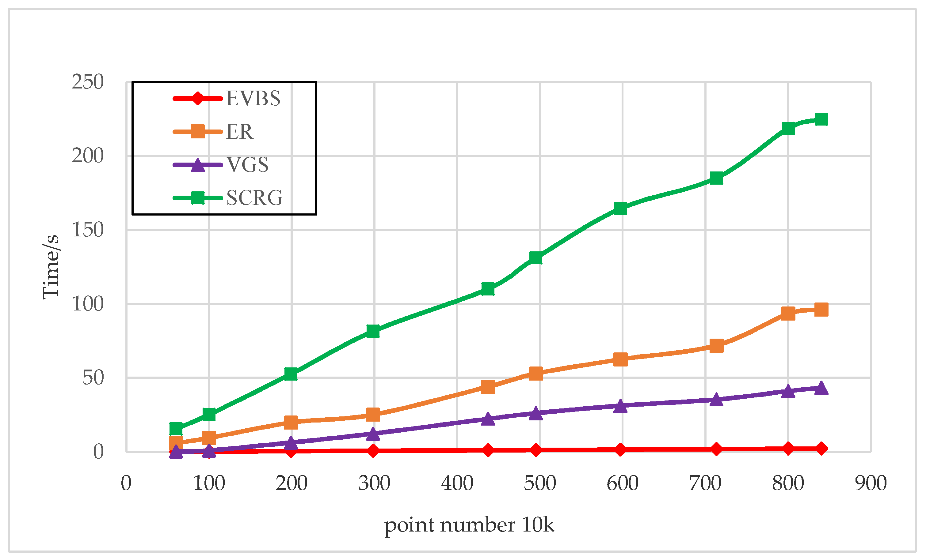
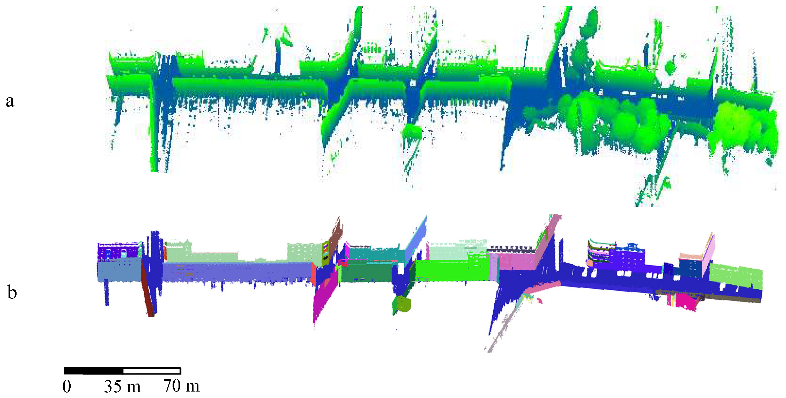
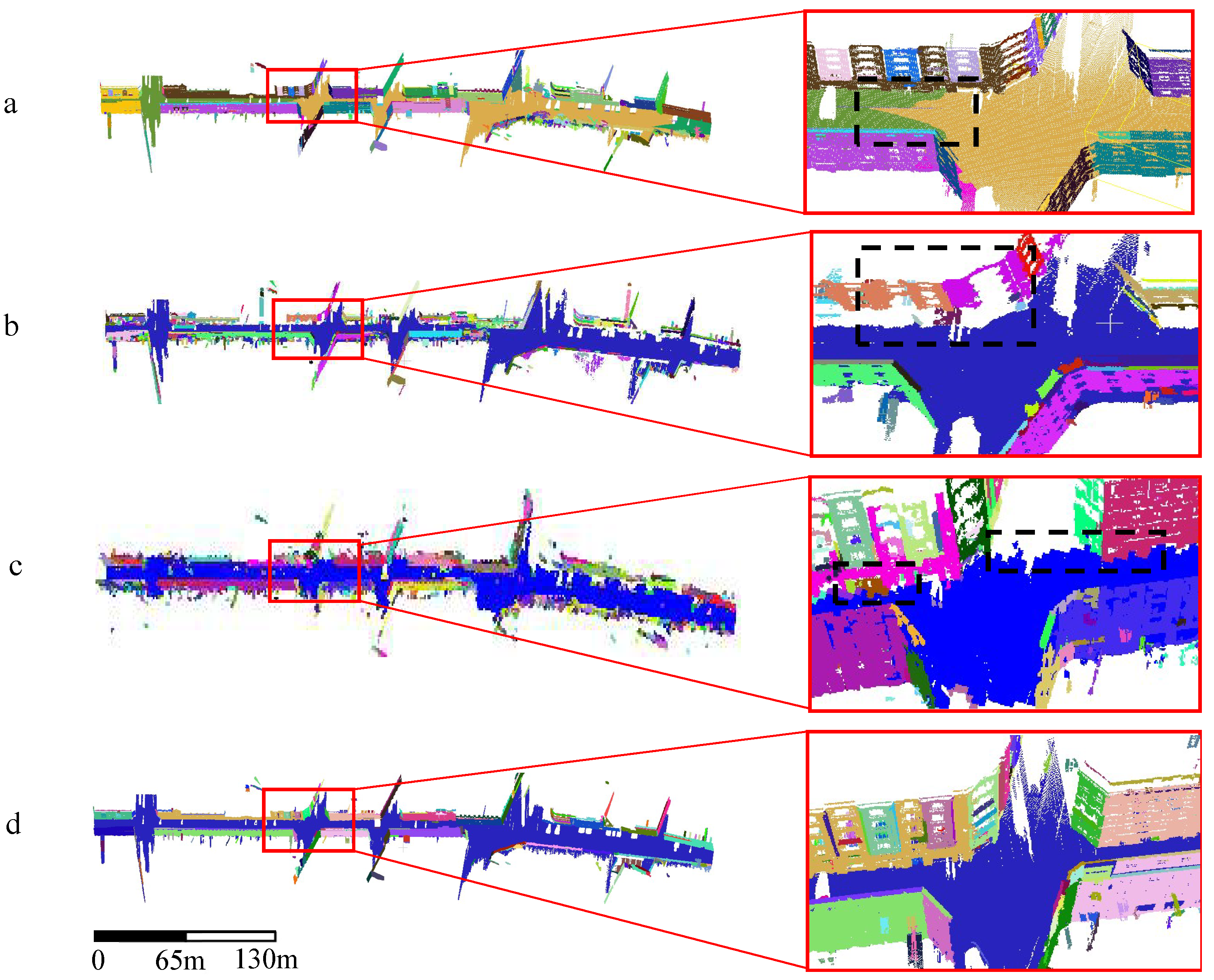
3.2. Results of Mobile Laser Scanner Data

The second group of experimental data was provided by the MATIS Laboratory of the French National Mapping Agency (IGN) and the Center for Mathematical Morphology in the IQmulus and Terra Mobilita Contest [34], as shown in Figure 12a. The data contain 13,500,158 points. A mobile laser scanner system developed at the IGN has been acquired by Stereopolis II. The mobile laser scanner system exhibits characteristics of fast acquisition of point clouds and wide acquisition range compared with a terrestrial laser scanner; however, mobile LiDAR point cloud data exhibit disadvantages of uneven density distributions and complex scenes [35,36]. According to the actual scene and the characteristics of mobile LiDAR point cloud data, in manual segmentation, a plane with a large area such as ground and building facades is regarded as the segmentation unit. The ground truth data obtained by manual segmentation is shown in Figure 12b.

The experimental results of handling mobile laser scanner data between the proposed and point-based algorithms are compared in Figure 13. The traditional point-based region growing algorithm SCRG only relies on the normal of the point as the constraint condition of region growing, thus resulting in serious under-segmentation and over-segmentation in segmented planes, as shown in Figure 13b. The RANSAC algorithm is a plane-fitting-based segmentation algorithm. Although the ER algorithm adds the restriction of a normal, it is still limited by the distance from a point to plane $d$. Therefore, when the road of the point cloud is extremely long and a slope exists, the segmentation result of the road will be incorrect, as shown in Figure 13a. The EVBS regards voxels as growing objects and voxel features as constraints, and it uses a region growing algorithm for segmentation to avoid the abovementioned problems; therefore, it can achieve a better segmentation effect, as shown in Figure 13d. The segmentation results are shown in

Table 3. Plane segmentation results using mobile laser scanner data.

	Precision	Recall	F1	Time (s)
ER	0.85	0.71	0.77	249.8
SCRG	0.66	0.29	0.40	295.1
VGS	0.86	0.57	0.69	49.3
EVBS	0.86	0.77	0.81	5.1

. As shown, the EVBS is superior to the other two algorithms in all metrics. The SCRG algorithm is disadvantageous for handling mobile LiDAR data, as the comprehensive metrics F1 is only 0.40. The F1 of the ER is 0.77, which is lower than that of our method (0.81). In terms of segmentation time, our algorithm requires only 5.1 s to complete all segmentations, while the other two algorithms require 249.8 s (ER) and 295.1 s (SCRG).

A voxel-based segmentation algorithm regards a voxel as a segmentation object, and the voxel at the junction of planes often contains points that belong to two or more planes. The VGS algorithm directly clusters voxels and does not process voxels separately at the junction of planes. Therefore, when the voxel resolution is large, a sawtooth point cloud plane boundary will appear, which results in non-ideal segmentations, as shown in Figure 13c. Because the residual value (represented by the normalized parameter herein) of voxels at the plane junction is large, our algorithm does not directly classify these voxels in the initial segmentation; subsequently, during refinement segmentation, we judge the relationship between each point in an unlabeled voxel and the segmented plane to avoid this phenomenon, thus improving segmentation, as shown in Figure 13d. As shown in the segmentation results in Table 3, the comprehensive metrics F1 of EVBS is 0.81, which is higher than 0.69 of the VGS. In terms of efficiency, the VGS algorithm requires 49.3 s to segment mobile laser scanner data, which is better than the general point-based plane segmentation algorithm; meanwhile, the EVBS only requires 5.1 s, which is better than the VGS. The experimental results show that the EVBS performs well in the plane segmentation of complex scene point cloud data.

4. Discussion

Herein, we presented a point cloud plane segmentation algorithm based on fast adjacent voxel search that aims to improve the efficiency and effect of point cloud plane segmentation. Based on the results of the aforementioned experiments, three issues must be addressed: voxel size setting, curved point cloud surface, and two parallel planes that are close to each other.

4.1. Voxel Size Setting

Our method uses a voxel as the segmentation object for point cloud plane segmentation. Unlike the method of adaptive voxel resolution used in [24], to better organize voxels and improve the efficiency and effectiveness of the algorithm, a voxel of uniform size is used in this study. To ensure a detailed segmentation, we set the size of the voxel to be the same as the minimum resolution of the voxels in [24]. Although this will increase the number of voxels, the efficient voxel organization method applied will ensure the efficiency of the algorithm. However, the voxel is extremely small, which results in fewer points in the voxel and unstable voxel features. According to our experiment, at least 200 points are required in a voxel to obtain stable voxel features. Using the same voxel size, the resolution of a point cloud affects the performance of the algorithm [37]. Although we can obtain the voxel resolution range according to Equation (15), the voxel size must still be set according to experience to achieve better segmentation in some cases (when we do not know the accuracy of the laser range measurement or the point cloud density).

In the terrestrial laser scanner data experiment, given the accuracy of laser range measurement of 4 mm, local point spacing of 3.2 mm, according to Equation (15), the number of points required for obtaining the angular accuracy of 6° is $k=\frac{m_0}{s}\frac{12}{m_{\alpha }}=\frac{4}{3.2}\frac{12}{\tan (6°)}\approx 143$ points. the voxel size should be larger than $d_I=\sqrt{k}\cdot s\approx 38mm$. In order to verify the influence of voxel size $d_I$ on the segmentation results, we used 0.03 m, 0.1 m, 0.15 m and 0.3 m to experiment. The experimental results are shown in Figure 14. Figure 14a is the segmentation result when $d_I=0.03$, in this case, the size of voxels is small, and the number of points divided into voxels is few. In the left voxelization result of Figure 14a, the average number of points in voxels is n = 213, which can calculate stable voxel features and divide them into correct planes. However, in the voxelization result of the roof point cloud on the right side of Figure 14a, the average number of points in the voxel is n = 52, which is sparsely and leads to unstable voxel features. It is easy to have a growth interruption problem in the voxel region growing when $d_I$ is too small, resulting in a plane being divided into multiple planes, which affects the result of plane segmentation. Due to the point cloud is divided into more voxels, the segmentation time is 81.5 s. Figure 14c shows the segmentation result when $d_I=0.15$.There is a blank area in the voxelization point cloud in Figure 14c, so this part of the point cloud should be divided into two planes Figure 15a. However, due to the large voxel size, the two parts of the boundary point cloud located in the adjacent voxels meet the region growing constraints, then they will be clustered into the same one plane as shown in Figure 15b. The same situation will occur at $d_I=0.3$, from Figure 14d, it can be seen that with the increase of voxel size, the level of detail of plane segmentation is also decreasing. Figure 14b shows the result of plane segmentation using threshold $d_I=0.1$ in Section 3.1. From the comparison of experimental results, it can be seen that the segmentation effect is the best by this threshold and consumes less time.

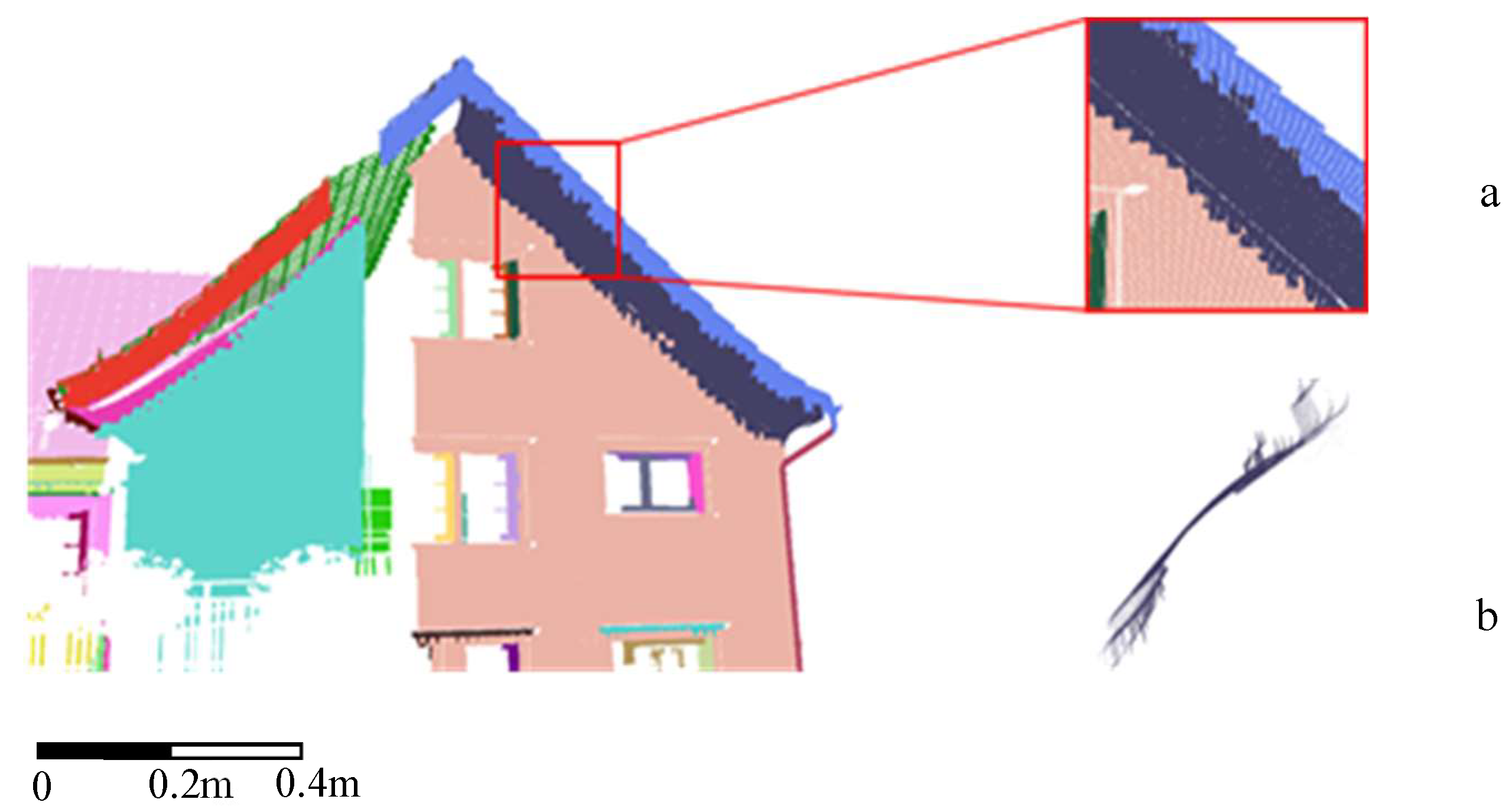
4.2. Curved Point Cloud Surface

The purpose of this algorithm is to segment a point cloud into point cloud planes. Sawtooth usually at the boundary between two connected planes which decreases the accuracy of plane segmentation in other methods [38,39,40]. In our paper a method of subdividing each point in an undivided voxel at the junction of two or more planes is adopted to segment point cloud data correctly, thus avoiding the sawtooth appearance of plane boundary points. However, in some scenes, a curved surface point cloud appeared. As shown in Figure 16, the point cloud at the junction of eaves and walls of the data in Section 3.1 is curved, and its boundary with the point cloud on the wall is not obvious. Therefore, the voxel residual value of this part is small and can grow to a certain plane in the initial growth, which will also result in the appearance of a sawtooth point cloud plane boundary, as shown in Figure 16a. However, in this study, we do not consider the segmentation of a curved surface point cloud. If the voxel resolution is set reasonably, this phenomenon will not be obvious and thus the segmentation results will not be affected significantly. Other circumstances, such as the segmentation of sphere, cylinder, cone, etc., will be the focus of our next stage research.

4.3. Two Parallel Planes Which are Close to Each Other

In the case of urban scenes, the abundant parallel facades bring difficulties to plane segmentation [41]. During voxel-based region growing, voxels with the same plane features are clustered into one group. For example, in Vo’s paper, a voxel normal is selected as the clustering condition for the voxel region growing [24]. However, according to the plane equation, it is insufficient to determine a plane by only the normal. When two planes are parallel and close to each other, it is easy to divide two planes into one plane according to the rule of region growing of adjacent voxels. Figure 17b shows two parallel planes that are close to each other. Figure 17c shows their side view and the result of voxelization. If only the normal of the voxel is selected as the growing constraint, the two grey voxels shown in Figure 17c will be clustered into one group; subsequently, these two parallel planes will be clustered into the same point cloud plane, as shown in Figure 17d. Therefore, according to the plane equation, we consider the spatial position relationship between the two voxels and add the constraint of continuity to cluster the voxel. When the spatial position of two adjacent voxels does not satisfy the set continuity threshold, the two voxels will not be clustered into the same plane; therefore, the parallel and adjacent planes will be separated correctly, as shown in Figure 17e.

5. Conclusions

Herein, an EVBS algorithm based on a fast adjacent voxel search was proposed. Compared with point-based and other voxel-based point cloud plane segmentation algorithms, the proposed EVBS algorithm demonstrated better segmentation and higher efficiency. Firstly, a highly efficient octree was used to organize a point cloud to replace a point cloud as a segmentation object. The voxels were binary coded such that 26 adjacent voxels could be obtained quickly, which is the basis of fast and accurate point cloud plane segmentation. Secondly, we improved the voxel-based region growing algorithm by selecting the rationality seed and growing criteria, which improved the plane segmentation accuracy. Lastly, in the initial segmentation, voxels with low flatness were not clustered. To solve the under-segmentation problem, we proposed a method of refining points in unlabeled voxels by judging the relationship between a point and a segmented plane. This method could prevent the sawtooth boundary of the segmented plane. Consequently, the recall rate and accuracy of the plane segmentation improved. Our algorithm was designed to afford a fast and accurate plane segmentation of a point cloud that had a large amount of data. It performed better in terms of accuracy and recall rate compared with traditional point-based segmentation algorithms (ER and SCRG) and an advanced voxel-based segmentation algorithm (VGS). This was verified from two groups of experiments. In terms of algorithm efficiency, our algorithm was less affected by the amount of point cloud data and was advantageous for handling a large amount of point data.

However, the focus of this method is only a plane object. It is interesting and significant to segment the point cloud with mixed objects efficiently, which will be our future work.

References

1. Liu, M. Robotic Online Path Planning on Point Cloud. IEEE Trans. Cybern. 2015, 46, 1217–1228. [Google Scholar] [CrossRef] [PubMed]
2. Boulch, A.; Guerry, J.; Le Saux, B.; Audebert, N. Snapnet: 3D point cloud semantic labeling with 2D deep segmentation networks. Comput. Graph. 2018, 71, 189–198. [Google Scholar] [CrossRef]
3. Hu, Q.; Wang, S.; Fu, C.; Yu, D.; Wang, W.T. Fine Surveying and 3D Modeling Approach for Wooden Ancient Architecture via Multiple Laser Scanner Integration. Remote Sens. 2016, 8, 270. [Google Scholar] [CrossRef]
4. Ma, L.; Favier, R.; Do, L.; Bondarev, E.; De With, P.H.N. Plane segmentation and decimation of point clouds for 3D environment reconstruction. In Proceedings of the IEEE Consumer Communications & Networking Conference (CCNC), Las Vegas, NV, USA, 11–14 January 2013; pp. 43–49. [Google Scholar]
5. Xu, Y.; Heogner, L.; Tuttas, S.; Stilla, U. A voxel- and graph-based strategy for segmenting man-made infrastructures using perceptual grouping laws: Comparison and evaluation. Photogramm. Eng. Remote Sens. 2018, 84, 377–391. [Google Scholar] [CrossRef]
6. Rebolj, D.; Pučko, Z.; Babič, N.Č.; Bizjak, M.; Mongus, D. Point cloud quality requirements for Scan-vs-BIM based automated construction progress monitoring. Autom. Constr. 2017, 84, 323–334. [Google Scholar] [CrossRef]
7. Xu, Y.; Hoegner, L.; Tuttas, S.; Stilla, U. Voxel- and graph-based point cloud segmentation of 3d scenes using perceptual grouping laws. ISPRS Ann. Photogramm. Remote Sens. Spat. Inf. Sci. 2017, 4, 43–50. [Google Scholar] [CrossRef]
8. Filin, S. Surface clustering from airborne laser scanning data. Int. Arch. Photogramm. Remote Sens. Spat. Inf. Sci. 2002, 34, 119–124. [Google Scholar]
9. Lerma, J.; Biosca, J. Segmentation and filtering of laser scanner data for cultural heritage. In Proceedings of the CIPA 2005 XX International Symposium, Torino, Italy, 26 September–1 October 2005; Volume 26. [Google Scholar]
10. Chehata, N.; David, N.; Bretar, F. Lidar data classification using hierarchical k-means clustering. In Proceedings of the ISPRS Congress, Beijing, China, 3–11 July 2008; pp. 325–330. [Google Scholar]
11. Wang, Y.; Hao, W.; Ning, X.; Zhao, M.; Zhao, M.H.; Zhang, J.L.; Shi, Z.H.; Zhang, X.P. Automatic segmentation of urban point clouds based on the Gaussian map. Photogram. Rec. 2013, 28, 342–361. [Google Scholar] [CrossRef]
12. Fischler, M.A.; Bolles, R.C. A paradigm for model fitting with applications to image analysis and automated cartography. Comm. ACM. 1981, 24, 381–395. [Google Scholar] [CrossRef]
13. Sveier, A.; Kleppe, A.L.; Tingelstad, L.; Egeland, O. Object detection in point clouds using conformal geometric algebra. Adv. Appl. Clifford Algebras 2017, 27, 1961–1976. [Google Scholar] [CrossRef]
14. Zeineldin, R.A.; El-Fishawy, N.A. Fast and accurate ground plane detection for the visually impaired from 3D organized point clouds. In Proceedings of the 2016 SAI Computing Conference (SAI), London, UK, 13–15 July 2016; pp. 373–379. [Google Scholar]
15. Torr, P.H.S.; Zisserman, A. MLESAC: A New Robust Estimator with Application to Estimating Image Geometry. Comput. Vis. Image Underst. 2000, 78, 138–156. [Google Scholar] [CrossRef]
16. Li, L.; Yang, F.; Zhu, H.; Li, D.; Li, Y.; Tang, L. An improved RANSAC for 3D point cloud plane segmentation based on normal distribution transformation cells. Remote Sens. 2017, 9, 433. [Google Scholar] [CrossRef]
17. Schnabel, R.; Wahl, R.; Klein, R. Efficient RANSAC for Point-Cloud Shape Detection. Comput. Graph. Forum 2007, 26, 214–226. [Google Scholar] [CrossRef]
18. Besl, P.J.; Jain, R.C. Segmentation through variable-order surface fitting. IEEE Trans. Pattern Anal. Mach. Intell. 1988, 10, 167–192. [Google Scholar] [CrossRef]
19. Rabbani, T.; Van Den Heuvel, F.; Vosselmann, G. Segmentation of point clouds using smoothness constraint. Int. Arch. Photogramm. Remote Sens. Spat. Inf. Sci. 2006, 36, 248–253. [Google Scholar]
20. Cai, Z.; Ma, H.; Zhang, L. A Building Detection Method Based on Semi-Suppressed Fuzzy C-Means and Restricted Region Growing Using Airborne LiDAR. Remote Sens. 2019, 11, 848. [Google Scholar] [CrossRef]
21. Tovari, D.; Pfeifer, N. Segmentation based robust interpolation-a new approach to laser data filtering. Remote Sens. Spat. Inf. Sci. 2005, 36, 79–84. [Google Scholar]
22. Woo, H.; Kang, E.; Wang, S.; Lee, K. A new segmentation method for point cloud data. Int. J. Mach. Tools Manuf. 2002, 42, 167–178. [Google Scholar] [CrossRef]
23. Su, Y.T.; Bethel, J.; Hu, S. Octree-based segmentation for terrestrial LiDAR point cloud data in industrial applications. ISPRS J. Photogramm. Remote Sens. 2016, 113, 59–74. [Google Scholar] [CrossRef]
24. Vo, A.V.; Truong-Hong, L.; Laefer, D.F.; Bertolotto, M. Octree-based region growing for point cloud segmentation. ISPRS J. Photogramm. Remote Sens. 2015, 104, 88–100. [Google Scholar] [CrossRef]
25. Lin, Y.; Wang, C.; Zhai, D.; Li, W.; Li, J. Toward better boundary preserved supervoxel segmentation for 3D point clouds. ISPRS J. Photogramm. Remote Sens. 2018, 143, 39–47. [Google Scholar] [CrossRef]
26. Marx, A.; Chou, Y.H.; Mercy, K.; Windisch, R. A Lightweight, Robust Exploitation System for Temporal Stacks of UAS Data: Use Case for Forward-Deployed Military or Emergency Responders. Drones 2019, 3, 29. [Google Scholar] [CrossRef]
27. Jiang, X.T.; Dai, N.; Cheng, X.S.; Zang, C.D.; Guo, B.S. Fast Neighborhood Search of Large-Scale Scattered Point Cloud Based on the Binary-Encoding Octree. Comput.-Aided Des. Comput. Graph. 2018, 30, 80–88. [Google Scholar]
28. Keling, N.; Yusoff, I.M.; Ujang, U.; Lateh, H. Highly Efficient Computer Oriented Octree Data Structure and Neighbours Search in 3D GIS. In Advances in 3D Geoinformation; Springer: Cham, Switzerland, 2017; pp. 285–303. [Google Scholar]
29. Nurunnabi, A.; Belton, D.; West, G. Robust Segmentation in Laser Scanning 3D Point Cloud Data. In Proceedings of the International Conference on Digital Image Computing Techniques and Applications (DICTA), Fremantle, Australia, 3–5 December 2012; pp. 1–8. [Google Scholar]
30. Xu, Y.; Tuttas, S.; Hoegner, L.; Stilla, U. Geometric primitive extraction from point clouds of construction sites using VGS. IEEE Geosci. Sens. Lett. 2017, 14, 424–428. [Google Scholar] [CrossRef]
31. Horvat, D.; Žalik, B.; Mongus, D. Context-dependent detection of non-linearly distributed points for vegetation classification in airborne lidar. ISPRS J. Photogramm. Remote Sens. 2016, 116, 1–14. [Google Scholar] [CrossRef]
32. Filin, S.; Pfeifer, N. Neighborhood systems for airborne laser data. Photogramm. Eng. Remote Sens. 2005, 71, 743–755. [Google Scholar] [CrossRef]
33. Hackel, T.; Savinov, N.; Ladicky, L.; Wegner, J.D.; Schindler, K.; Pollefeys, M. SEMANTIC3D.NET: A new large-scale point cloud classification benchmark. In Proceedings of the ISPRS Annals of the Photogrammetry, Remote Sensing and Spatial Information Sciences, Hannover, Germany, 6–9 June 2017; pp. 91–98. [Google Scholar]
34. Vallet, B.; Brédif, M.; Serna, A.; Marcotegui, B.; Paparoditis, N. TerraMobilita/iQmulus urban point cloud analysis benchmark. Comput. Gr. 2015, 49, 126–133. [Google Scholar] [CrossRef]
35. Li, Y.; Li, L.; Li, D.; Yang, F.; Liu, Y. A density-based clustering method for urban scene mobile laser scanning data segmentation. Remote Sens. 2017, 9, 331. [Google Scholar] [CrossRef]
36. Cabo, C.; Ordoñez, C.; García-Cortés, S.; Martínez, J. An algorithm for automatic detection of pole-like street furniture objects from mobile laser scanner point clouds. ISPRS J. Photogramm. Remote Sens. 2014, 87, 47–56. [Google Scholar] [CrossRef]
37. Deschaud, J.E.; Goulette, F. A fast and accurate plane detection algorithm for large noisy point clouds using filtered normals and voxel growing. In Proceedings of the 3D Processing, Visualization and Transmission Conference (3DPVT2010), Paris, France, 17–20 May 2010. [Google Scholar]
38. Feng, C.; Taguchi, Y.; Kamat, V.R. Fast plane extraction in organized point clouds using agglomerative hierarchical clustering. In Proceedings of the 2014 IEEE International Conference on Robotics and Automation (ICRA), Hong Kong, China, 31 May–7 June 2014; pp. 6218–6225. [Google Scholar]
39. Liu, P.; Li, Y.; Hu, W.; Ding, X. Segmentation and Reconstruction of Buildings with Aerial Oblique Photography Point Clouds. Int. Arch. Photogramm. Remote Sens. Spat. Inf. Sci. 2015, XL-7/W4, 109–112. [Google Scholar] [CrossRef]
40. Pan, Y.; Dong, Y.; Wang, D.; Chen, A.; Ye, Z. Three-dimensional reconstruction of structural surface model of heritage bridges using UAV-based photogrammetric point clouds. Remote Sens. 2019, 11, 1204. [Google Scholar] [CrossRef]
41. Xu, Y.; Boerner, R.; Yao, W.; Hoegner, L.; Stilla, U. Automated coarse registration of point clouds in 3D urban scenes using voxel based plane constraint. ISPRS Ann. Photogramm. Remote Sens. Spat. Inf. Sci. 2017, IV-2/W4, 185–191. [Google Scholar] [CrossRef] [Green Version]
Figure 1. The whole process of segmentation algorithm.
Remotesensing 11 02727 g001
Figure 2. A highly efficient binary encoding octree data structure. (a) A voxel coded according to the X, Y, and Z axes with 0 or 1, (b) binary coding of octree in level 1, and (c) binary coding of octree in level 2 which is part of (b).
Remotesensing 11 02727 g002
Figure 3. Procedure of searching 26 adjacent voxels. (a) Voxels generated by point clouds, (b) 26 adjacent voxels, (c) adjacent voxel search results, and (d) point cloud in adjacent voxels.
Remotesensing 11 02727 g003
Figure 4. Residual feature estimation of voxel.
Remotesensing 11 02727 g004
Figure 5. Voxel smoothness constraint. (a) Voxels A and B satisfy smoothness constraint θ A B θ t h and (b) voxels A and B do not satisfy smoothness constraint θ A B > θ t h .
Remotesensing 11 02727 g005
Figure 6. Voxel continuity constraint. (a) Voxels A and B satisfy continuity constraint O 1 O 2 · N 1 < φ t h and (b) voxels A and B do not satisfy continuity constraint O 1 O 2 · N 1 > φ t h .
Remotesensing 11 02727 g006
Figure 7. Process for handling under-segmentation. (a) Results of coarse point cloud segmentation; (bd) are cases of under-segmentation, (e) schematic of unlabeled voxel segmentation, (f) a voxel at the junction of two planes cannot cluster into anyone plane, and (g) results of unlabeled voxel segmentation.
Remotesensing 11 02727 g007
Figure 8. Terrestrial light detection and ranging (LiDAR) data. (a) Point cloud published by Zurich Federal Institute of Technology (ETH) Zurich, and (b) ground truth data obtained by manual segmentation.
Remotesensing 11 02727 g008
Figure 9. Segmentation results of terrestrial laser scanner data. (a) Segmentation results of efficient RANSAC algorithm (ER) algorithm, (b) segmentation results of the region growing algorithm (SCRG) algorithm, (c) segmentation results of VGS algorithm, and (d) segmentation results of the encoding voxel-based segmentation (EVBS) algorithm.
Remotesensing 11 02727 g009
Figure 10. Details of result comparison of terrestrial laser scanner data. (a) Details of segmentation results of VGS, and (b) details of segmentation results of the EVBS algorithm.
Remotesensing 11 02727 g010
Figure 11. Execution time comparison of the three algorithms with different data sizes.
Remotesensing 11 02727 g011
Figure 12. Mobile laser scanner data. (a) Mobile laser scanner point cloud obtained by the MATIS Laboratory, and (b) ground truth data obtained by manual segmentation.
Remotesensing 11 02727 g012
Figure 13. Segmentation results of mobile laser scanner data. (a) Segmentation results of ER algorithm, (b) segmentation results of SCRG algorithm, (c) segmentation results of VGS, and (d) segmentation results of the EVBS.
Remotesensing 11 02727 g013
Figure 14. Segmentation results and partial voxelization results of different sizes of d I . (a) experiment results when d I = 0.03 , cost time 81.5 s, (b) experiment results when d I = 0.1 , cost time 7.8 s, (c) experiment results when d I = 0.15 , cost time 7.0 s, and (d) experiment results when d I = 0.3 , cost time 5.8 s.
Remotesensing 11 02727 g014
Figure 15. The segmentation result by using different voxel sizes to process the red point cloud. (a) segmentation result of small voxel size, two planes have been segmented and (b) segmentation result of bigger voxel size, only one plane has been segmented.
Remotesensing 11 02727 g015
Figure 16. Sawtooth boundary in curved surface point cloud. (a) Details of sawtooth point cloud, and (b) bending section of sawtooth point cloud.
Remotesensing 11 02727 g016
Figure 17. Managing a parallel plane. (a) Original point cloud of terrestrial laser scanner data, and (b) two parallel planes that are close to each other, (c) side view of (b) and the result of voxelization, (d) segmentation result of (b) without continuity constraint, and (e) segmentation result of (b) with continuity constraint.
Remotesensing 11 02727 g017