Debris Flow Susceptibility Mapping Using Machine-Learning Techniques in Shigatse Area, China


1
School of Automation, Nanjing University of Information Science & Technology, Nanjing 210044, China
2
School of Computer and Software, Nanjing University of Information Science & Technology, Nanjing 210044, China
3
Center for Space and Remote Sensing Research, National Central University, Taoyuan 32001, Taiwan
*
Authors to whom correspondence should be addressed.
Remote Sens. 2019, 11(23), 2801; https://0-doi-org.brum.beds.ac.uk/10.3390/rs11232801
Submission received: 8 October 2019
/
Revised: 5 November 2019
/
Accepted: 21 November 2019
/
Published: 27 November 2019
(This article belongs to the Special Issue Earth Observations for Environmental Sustainability for the Next Decade)
Abstract
:Debris flows have been always a serious problem in the mountain areas. Research on the assessment of debris flows susceptibility (DFS) is useful for preventing and mitigating debris flow risks. The main purpose of this work is to study the DFS in the Shigatse area of Tibet, by using machine learning methods, after assessing the main triggering factors of debris flows. Remote sensing and geographic information system (GIS) are used to obtain datasets of topography, vegetation, human activities and soil factors for local debris flows. The problem of debris flow susceptibility level imbalances in datasets is addressed by the Borderline-SMOTE method. Five machine learning methods, i.e., back propagation neural network (BPNN), one-dimensional convolutional neural network (1D-CNN), decision tree (DT), random forest (RF), and extreme gradient boosting (XGBoost) have been used to analyze and fit the relationship between debris flow triggering factors and occurrence, and to evaluate the weight of each triggering factor. The ANOVA and Tukey HSD tests have revealed that the XGBoost model exhibited the best mean accuracy (0.924) on ten-fold cross-validation and the performance was significantly better than that of the BPNN (0.871), DT (0.816), and RF (0.901). However, the performance of the XGBoost did not significantly differ from that of the 1D-CNN (0.914). This is also the first comparison experiment between XGBoost and 1D-CNN methods in the DFS study. The DFS maps have been verified by five evaluation methods: Precision, Recall, F1 score, Accuracy and area under the curve (AUC). Experiments show that the XGBoost has the best score, and the factors that have a greater impact on debris flows are aspect, annual average rainfall, profile curvature, and elevation.
1. Introduction
Debris flows involve gravity-driven motion of solid-fluid mixtures with abrupt surge fronts, free upper surfaces, variably erodible basal surfaces, and compositions that may change with position and time [1]. They can cause great damage to the safety of people’s lives and property, public facilities and ecological environment. Due to the harsh natural environment and deforestation caused by over-exploitation of human beings, Shigatse is a typical area with active debris flows in the Tibet Autonomous Region. Debris flows can cause very high damages because the study area is densely populated. Therefore, mitigating and reducing the disasters caused by debris flows are critical to the local authorities. Most of Shigatse mountainous area is inaccessible and characterized by very steep slope such that it is very difficult to carry out field surveys. The installation and maintenance of sufficient monitoring facilities in these areas are also very challenging. Therefore, zoning debris flow susceptibility (DFS) maps through spatial data can be used to prevent and mitigate casualties and economic losses caused by debris flow events.
Susceptibility mapping of debris flow is prominent for early warning and treatments of regional debris flows. DFS assessment is based on the spatial characteristics of debris flow events and relevant factors (topography, soil, vegetation, human activities and climate). It aims to estimate the spatial distribution of future debris flow probability in a given area [2]. Some studies have discussed and analyzed debris flows in the study area [3,4], focusing on the residential settlements and vicinity of roads. Assessing the susceptibility of debris flows in the whole study area is difficult due to the vast size of land (exceeding 180,000 square kilometers). The detailed spatial information on the debris flow triggering factors is also quite limited. In this case, satellite remote sensing has good application prospects because it can describe the characteristics of a large area, such as terrain, vegetation, and climate of the place where debris flow events occur. Therefore, compared with the traditional field geological survey, which requires a lot of work and resources, data from remote sensing represented in a GIS environment can fill the gap of on-site monitoring data. That is, it can be applied for the DFS researches in a more effective and economical way.
In recent years, GIS and remote sensing data have been used to conduct many studies of disasters in mountains. Researchers built their methodology analyzing data of known occurred debris flows and tested it through unknown debris flow events. Gregoretti et al. [5] proposed a GIS-based model tested against field measurements for a rapid hazard mapping. Kim et al. [6] used a high-resolution light detection and ranging (LiDAR) digital elevation model to calculate the volume of debris flows. Kim et al. [7] developed a GIS-based real-time debris flow susceptibility assessment framework for highway sections. Alharbi et al. [8] presented a GIS-based methodology for determining initiation area and characteristics of debris flow by using remote sensing data. At present, the DFS assessment methods can be mainly divided into two categories: qualitative and quantitative models. The qualitative model assigns a weight (0–1) to each debris flow triggering factor based on expert experience and knowledge or heuristics to assess the DFS [9]. Common qualitative analysis methods include fuzzy logic [10], analytic hierarchy [11] and network analysis [12] and so on. While these models have achieved a lot in the study of debris flows, they still suffer for some shortcomings, such as a high degree of subjectivity and limited applicability to specific areas [13].
Quantitative methods usually include two types: deterministic and statistical models based on physical mechanisms. Deterministic methods are used to study the physical laws of debris flows and establish the corresponding models to simulate the DFS [14]. The disadvantages of these models are in that they require detailed inspection data for each slope. Thus, they are only suitable for smaller areas. Statistical models are data-driven. The DFS assessment from them combines the past debris flow events with environmental characteristics. It is assumed that the environmental characteristics of the past debris flows events will lead to debris flows in the future. The models for the DFS quantitative assessment include information model [15], evidence weight method [16], frequency ratio [17] and so on.
In recent years, data mining and machine learning techniques have also received extensive attention because they can more accurately describe the nonlinear relationship between DFS and triggering factors [18], and there is no special requirement for the distribution of triggering factors. Machine learning algorithms are often superior to traditional statistical models [19] for the following reasons. First of all, machine learning can adapt to larger datasets, while traditional statistical learning methods are more suitable for small datasets. Secondly, machine learning has better controllability and extensibility than traditional statistical models. Moreover, traditional statistical models are in general limited to certain requirements and assumptions on data, whereas machine learning methods are not. In the past three decades, common machine learning methods used for studying DFS mapping include back propagation neural network (BPNN) [20], decision tree (DT) [21], Bayesian network [22], and support vector machine [23]. With the advancement of researches, more and more models have been developed with better fitting performance. Under such circumstances, continuous verification and evaluation are still necessary for constructing and selecting a DFS evaluation model. Therefore, comparisons among various models to investigate DFS have become hot topics in academia. Since the information about debris flow occurrence is very limited and different, stability and accurate predictive power are the primary requirements for selecting the appropriate method to achieve better modeling results.
Among machine learning methods, BPNN is widely used because it carries the excellent nonlinear fitting and complex learning abilities to extract the complex relationship between debris flow triggering factors and DFS [24]. Convolutional neural network, a classical deep learning method, has been rapidly developed in the past decade and is widely used in pattern recognition and medicine It is generally used for classification and recognition of two-dimensional images. In recent years, artificial intelligence scholars have made the convolutional neural network one-dimensional, so as to perform the speech recognition [25], fault diagnosis [26] and data classification [27]. As an end-to-end model, the one-dimensional convolutional neural network can extract and classify different characteristics of debris flows directly from raw data without expert guidance. DT is another powerful prediction model with three major advantages: the model is easy to build; the final model is easy to interpret; and the model provides clear information about the relative importance of input factors [28]. These advantages have motivated researchers to develop new DT models to better utilize the debris flow information. At the same time, integrated learning algorithms based on decision trees have also been widely concerned. Among them, the more representative ones are bagging and boosting. Kadavi et al. [29] used four integrated algorithms: Adaboost, Bagging, LogitBoost, and Multiclass classifier to calculate and plot the DFS map. They proved that the Multiclass classifier had the best performance by verifying the AUC value of the test set.
Due to the complex terrain, geology and other mountain conditions in the study area, the multi-source and multi-data are used as much as possible to characterize the terrain and geological conditions of debris flows. Although machine learning methods have been demonstrated to achieve results with satisfactory to some extent, this paper further discusses whether they can be applied to examine the DFS. Its most important contributions are described as follows. (a) We collected debris flow events data and a variety of original remote sensing data related to topographic factors, such as soil factors, human factors and vegetation factors, and performed pre-processing operations, including projection, registration and sampling based on remote sensing and GIS technology (ArcGIS v.10.2 software). (b) We obtained the characteristics of the study area where debris flow occurred and used the data generation algorithm to merge the collected debris flow events data. (c) Based on the Python language, using the keras framework and the scikit-learn module, five DFS models (BPNN, 1D-CNN, DT, RF, and XGBoost) were constructed for the training set. The applicability of these models was examined for the Shigatse region. It is notable that this is the first comparative experiment of XGBoost and 1D-CNN in the study of DFS. (d) Cross-validation methods were used to compare the performance of artificial neural networks and tree-based models to reduce the bias and variance. (e) Statistical analyses of the comparative algorithm were done to verify whether the performance is significantly different. (f) The test set was used to evaluate the models’ prediction ability in combination with the five evaluation methods of classical Recall, Precision, F1 score, Accuracy, and AUC [30]. (g) At the end of the study, the tree-based “feature importance” ranking was used to evaluate the main characteristic factors affecting the DFS.
2. Material and Methods
2.1. Study Area
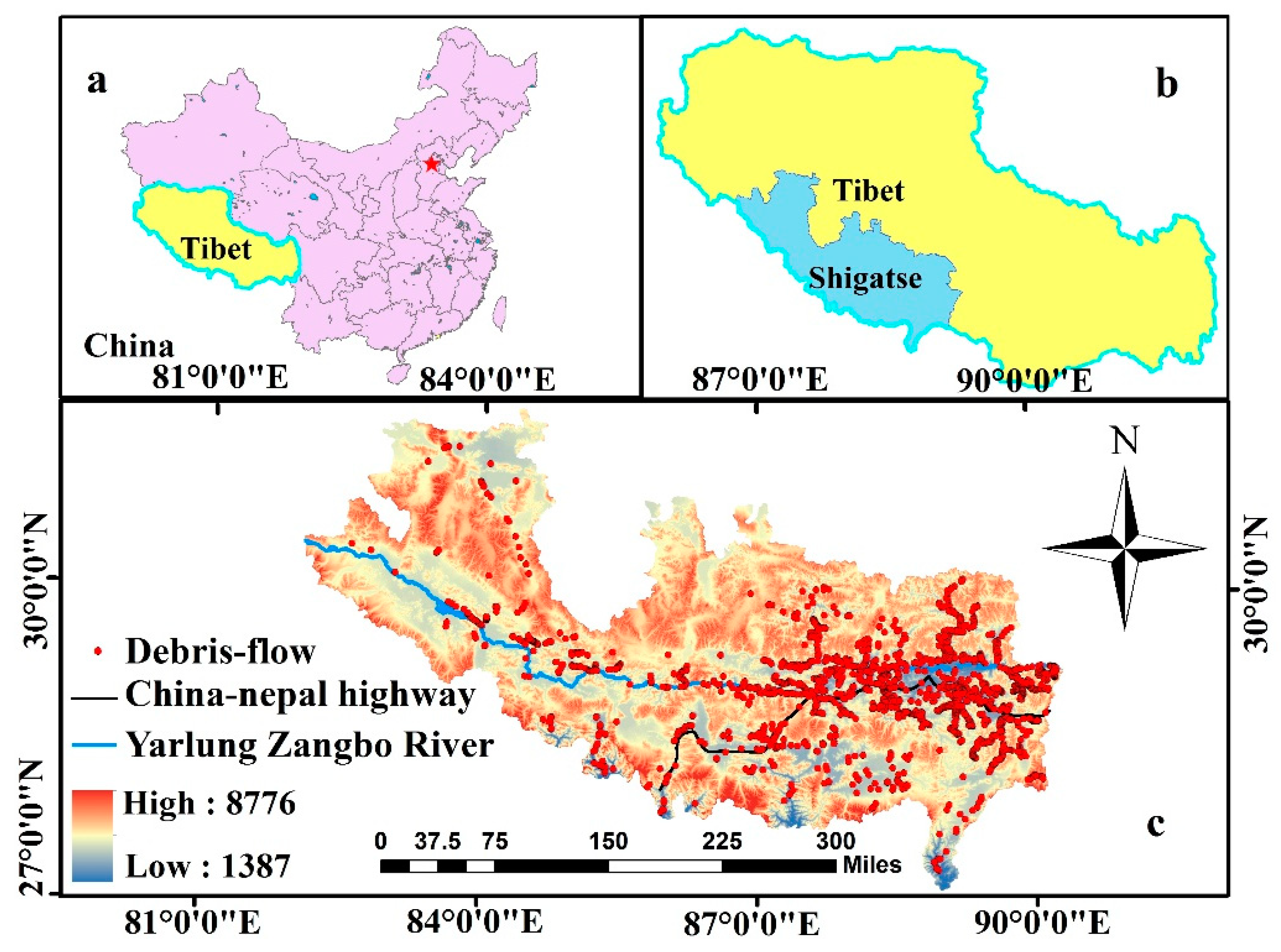
The study area covers an area of 182,000 square kilometers in the southwestern part of China. It is located in the southwest of the Tibet Autonomous Region (27°23′~31°49′N, and 82°00′~90°20′E). As shown in Figure 1, the Shigatse area is mainly located between the central Himalayas and central part of the Gangdise-Nyqinqin Tanggula Mountains. Its elevation is high in the northern part and southern part, including the southern Tibetan Plateau and Yarlung Zangbo River basin. The overall terrain of the Shigatse region is complex and diverse, mainly consisting of mountains, wide valleys and lake basins with a maximum elevation of over 8700 m. The study area belongs to semi-arid monsoon climate zone of inland plateau. It is featured with dry climate, less precipitation, rainy season coincident with hot season, and annual average sunshine hours of 3240 h.
The transportation mainly includes three main lines: China-Nepal (Zhongni) Highway, 318 National Road and Largo Railway passing through the study area. The geological disasters in the study area are serious, mainly including debris flows, rock collapses, and landslides. Among them, the debris flow is the most common one. A large number of debris flows exist in many parts of the study region. They directly threaten the safety of the three major transportation lines and residents’ lives and properties. According to the collected data and previous studies [31], the debris flows in the study area are mostly caused by heavy rain.
2.1.1. Debris Flow Dataset
Collection and analysis of debris flow event datasets are prerequisites for the DFS assessment. There are 1944 debris flow sites in the study area from 1998 to 2008. Each case includes information obtained from field disaster investigation, such as time, debris flow susceptibility level, and geographic location. The information on debris flows is provided by the Tibet Meteorological Bureau. These events can be viewed through the geological cloud portal [32].
2.1.2. Debris Flow Triggering Factors
It is significant to analyze the environmental characteristics of the debris flow events for the DFS estimation. Due to the complexity of the environment and various development stages of debris flows, the causes of debris flows are controversial. Researchers have done a lot of studies on the relationship between debris flows and triggering factors, such as topography, soil, climate, and human activities. Therefore, we have classified 15 environmental factors into five categories as shown in Table 1.
Topographic factors that include elevation, slope, aspect, and curvature are extracted from the Shuttle Radar Topography Mission Digital Elevation Model (SRTM DEM) using the ArcGIS platform [33]. The vegetation coverage is represented by the normalized difference vegetation index (NDVI), calculated from the obtained 2000–2008 MODIS images and averaged to generate the thematic layer of the annual average NDVI. Rainfall data are collected from the Tropical Rainfall Measurement Task (TRMM) [34]. We use a rainfall dataset (No: 3B42v7) with a time interval of three hours and a spatial resolution of 0.25 degree during 1998–2008 to construct a thematic layer of annual average precipitation. The 15 types of land use information layers are provided by National Earth System Science Data Sharing Infrastructure, National Science & Technology Infrastructure of China (http://www.geodata.cn) [35,36]. In addition, the road vector data provided by OpenStreetMap (OSM) (https://www.openstreetmap.org/#map=11/22.3349/113.76000) is used to calculate the distance from the road. Soil factors are provided by the Resource and Environmental Science Data Center (RESDC) of the Chinese Academy of Sciences.
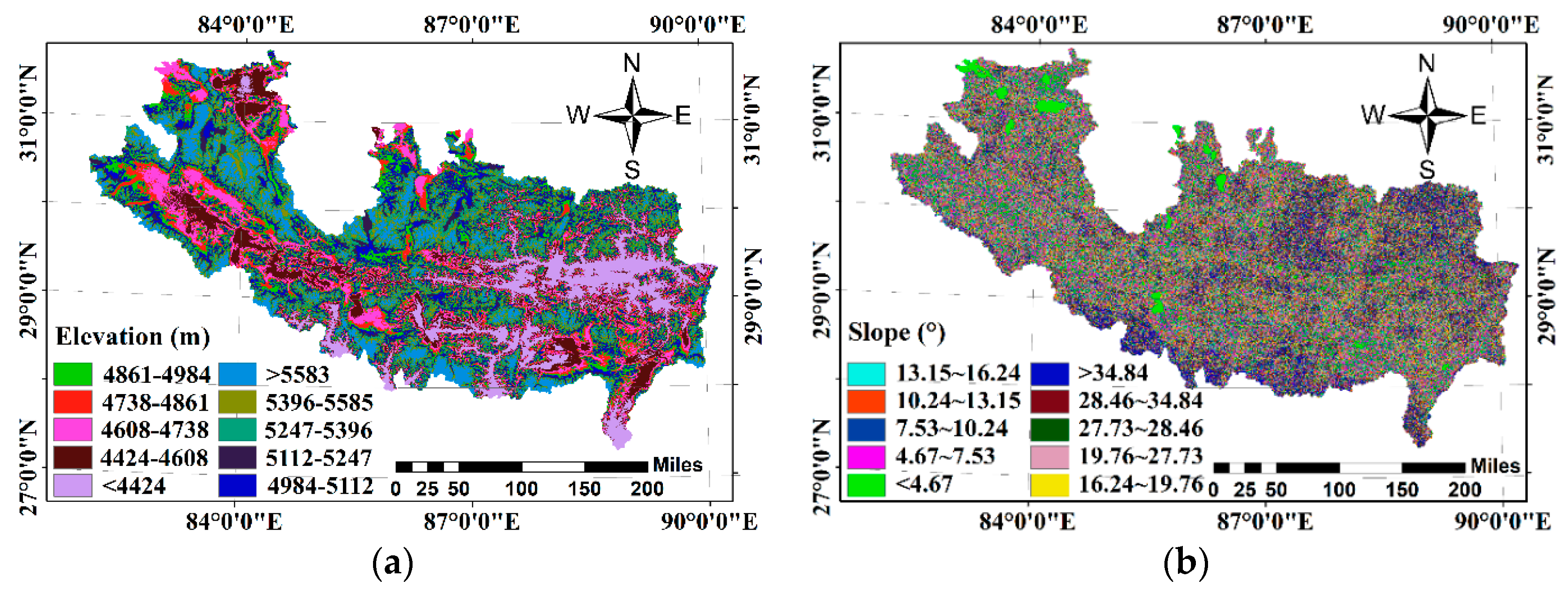
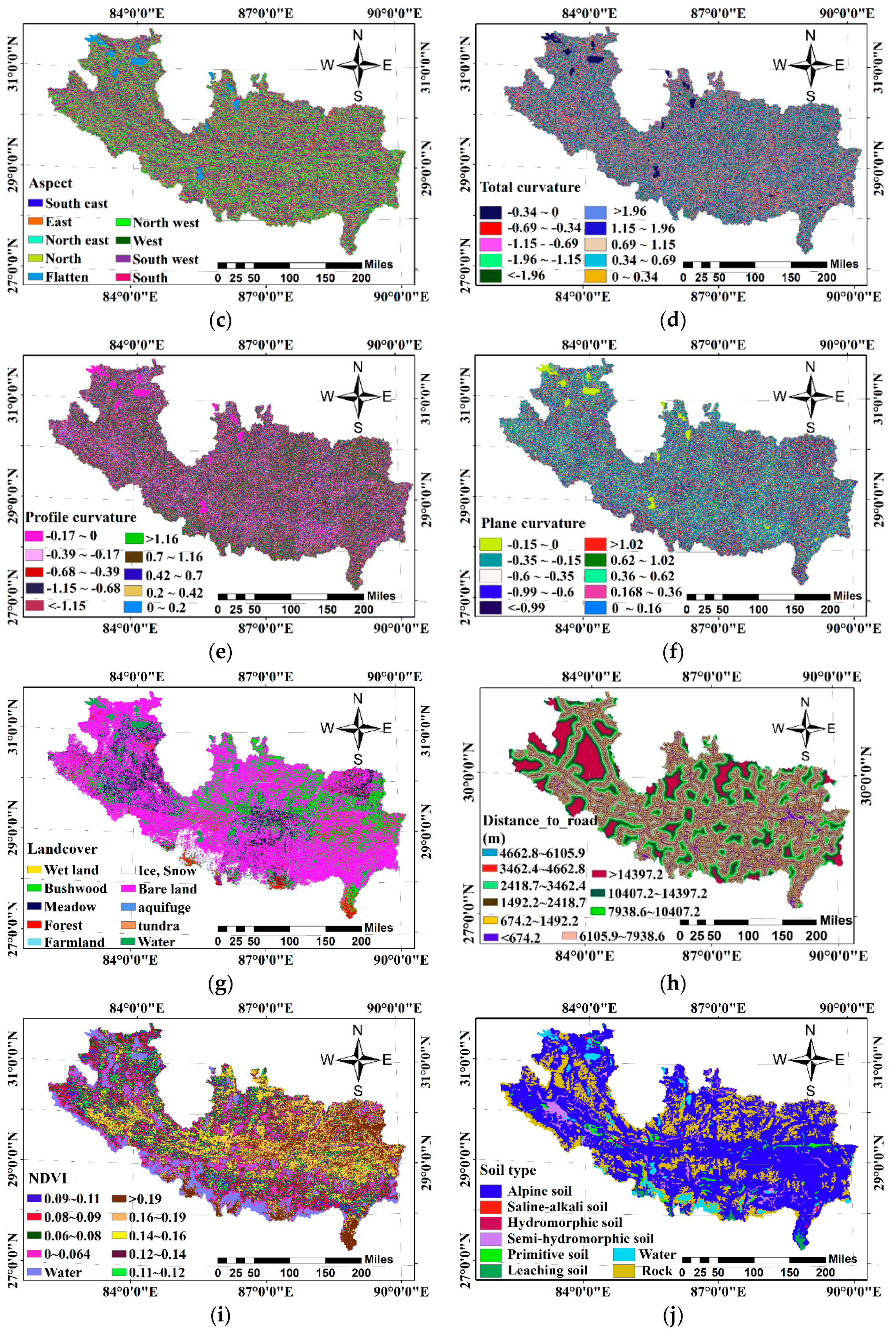
Higher resolution is conducive to the topographic analysis of single-ditch debris flow, but in this work, our research focuses on the use of multiple attribute factors to analyze the disaster susceptibility of the entire study area. Golovko [2] and Ahmed [9] believe that 30M resolution Digital Elevation Model (DEM) can be used for the analysis of the susceptibility to mountain disasters. Therefore, DEM data with a pixel size of 30 m is used (Figure 2a). The slope angle is a fundamental factor calculated by the DEM data and the range of it obtained by statistics is wide (0–89°) (Figure 2b). The aspect of the slope is another key factor affecting the DFS. Because the slope surface in different directions is exposed to the wind and rain in different degrees. The aspect thematic layers are reclassified into nine categories: flat (−1), north (337.5–360°, 0–22.5°), north-east (22.5–67.5°), east (67.5–112.5°), south-east (112.5–157.5°), south (157.5–202.5°), south-west (202.5–247.5°), west (247.5–292.5°), and north-west (292.5–337.5°) (Figure 2c). The second derivative of the slope, i.e., the curvature, helps us understand the characteristics of the basin runoff and erosion processes. In this study, three curvature functions are used to show the shape of the terrain (Figure 2d–f). They are the curvature of the profile, the curvature of the plane, and the total curvature of the surface defined as the curvature of the maximum slope, the curvature of the contour, and the combination of the curvatures, respectively.
Human activities affect the geographical environment, which in turn influences the occurrence of debris flows. The land cover thematic map shows how human production can change natural land, and 14 land use types including farmland and forest can be identified (Figure 2g). The DFS assessment often takes the distance from the road into account, because the road construction and maintenance cause certain change and damage to the local morphology. This variable is calculated by using the Euclidean distance calculation technique in the spatial analysis tool of ArcGIS 10.2 (Figure 2h).
The vegetation coverage is one of the important parameters to evaluate the DFS. NDVI extracted from remote sensing images is a commonly used vegetation index for inferring the vegetation density. It is very sensitive to the presence of chlorophyll on vegetation surface (Figure 2i). We calculated the NDVI value using the following formula:
where NIR and RED represent the near-infrared and red-band, respectively, and they are the second and first channels of the MODIS image. The NDVI value ranges between −1 and 1. The negative value indicates that the ground cover is an object highly reflective to visible light such as clouds, snow, water, etc. 0 means bare land. A positive value represents a vegetation coverage area and it increases with the vegetation coverage density.
NDVI = (NIR − RED)/(NIR + RED)
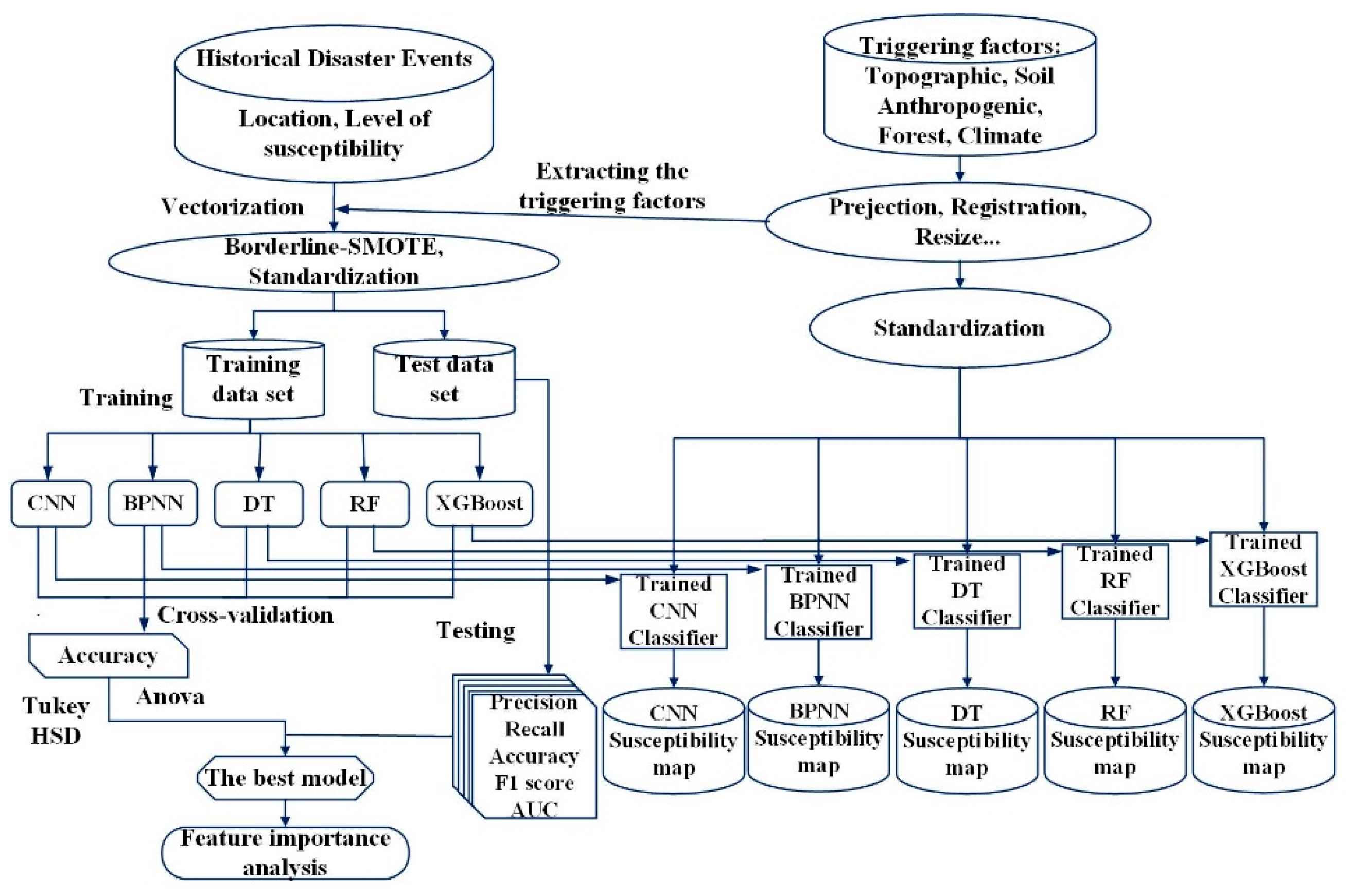
Debris flows are usually influenced by changes in humidity caused by rainfall infiltration. Permeability can be expressed by soil type (Figure 2j), soil texture (Figure 2k–m) and soil erosion (Figure 2n). Since the particle distribution determines the shape of soil water characteristic curve and affects the soil hydraulic characteristics, the soil type and texture have a great influence on the DFS. Most of the study area is covered by alpine soil, including grass mat soil, cold soil, and frozen soil. According to statistics, most of the alpine soil is brown and has a strong acidity. The alpine soil is mainly composed of silt, sand and clay fine sand, and has fast permeable and low moisturized ability. Soil erosion is sometimes used as a synonym for soil and water loss, and areas with severe erosion are susceptible to debris flows. The external causes of soil erosion are mainly hydro, wind, and freeze-thaw. Clearly, fragile soil characteristics accompanied by concentrated rainfall usually result in debris flows.
Rainfall is the main factor leading to debris flows. The study area is affected by the monsoon climate with rare precipitation and an annual average precipitation less than 1300 mm (Figure 2o). However, statistical analyses of the geological hazard points occurring in the study area show that heavy rain and continuous rainfall are important external factors leading to geological disasters in the Shigatse area.
2.2. Methods
The main purpose of our research is to fit the relationship between the triggering factors and occurrence of debris flows. The problem can be expressed as a multi-class classification. Given a set of input quantities, the classification model attempts to label the DFS level for each pixel in the study area. The input quantities to the models are the triggering factors of the debris flow events that were collected by the local Chinese Geological Survey researchers after many years of field investigation. According to the researchers’ investigation of the debris flow sites, we obtain the values of 15 triggering factors at the corresponding positions through the value extraction function of ArcGIS v10.2 software. That is, the input of the model is a one-dimensional vector form [×1, ×2, …, ×15]. The output value of the model is the DFS level, indicating the occurrence probability of debris flows. The division criteria of regional DFS are based on the detailed survey and specification of landslide collapse debris flows by the China Geological Survey as shown in Table 2.
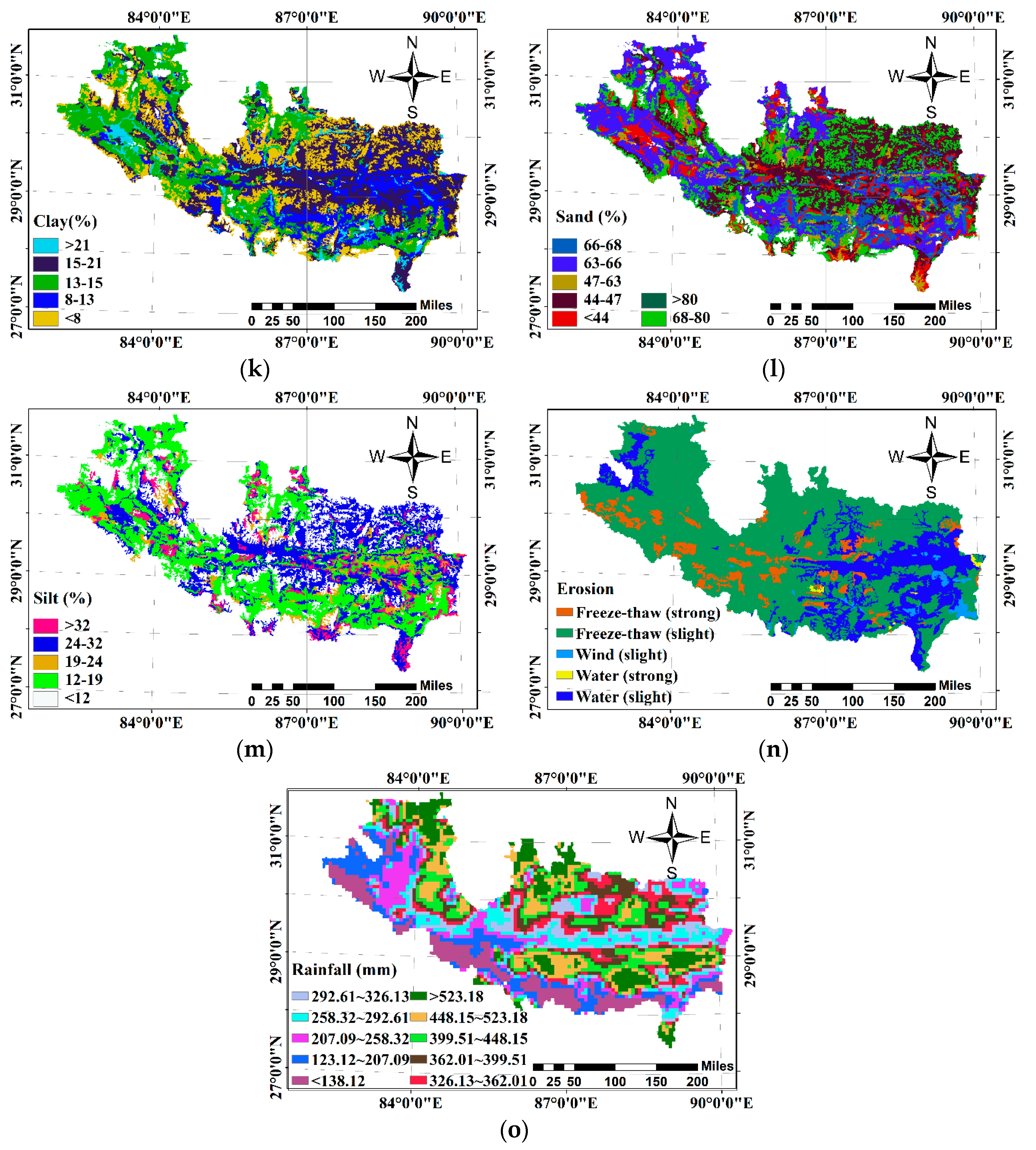
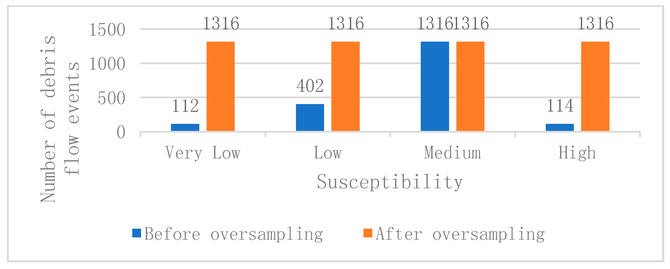
According to statistics, the number of moderately susceptible units in the study area is much higher than that of the other susceptible grades (Figure 3). Therefore, before constructing a debris flow assessment model, the oversampling technique Borderline-SMOTE algorithm should be used to eliminate the classification imbalance in the dataset. The number of each debris flow susceptibility level after oversampling is shown in Figure 3. The original dataset is divided into training sets and test sets according to a percentage of 75 and 25%, respectively. The training set of the debris flow triggering factors is used to learn the ability to fit the actual DFS classification, and the validation set is used for adjusting the model parameters to prevent over-fitting or under-fitting. In this study, five DFS models have been established using DT, BPNN, 1D-CNN, RF, and XGBoost. Among them, the DT and BPNN have been the most commonly used machine learning models in the past few decades. The one-dimensional convolutional neural network (1D-CNN) has achieved remarkable results in one-dimensional signal processing, such as fault diagnosis and speech recognition. RF is based on the DT. It is a typical integrated algorithm in machine learning algorithms. The XGBoost is also a tree-based integration model, which counts on the residuals generated by the last iteration. To the best of our knowledge, the XGBoost and 1D-CNN have not been used for the DFS. Based on the above introductions, the research framework for the DFS in Shigatse is shown in Figure 4.
In addition, we have also implemented other traditional machine learning algorithms, such as support vector machine, logistic regression, and naive Bayesian model, but the results are disappointing. Therefore, these methods are not introduced here. The following part is a brief introduction to the data sampling generation algorithm and five classifiers used in this paper.
2.2.1. Borderline-SMOTE
It is well known that in the model training process, when a certain class in the classified data set is of a high proportion, the classifier performance will be seriously affected. Synthetic Minority Oversampling Technique is often referred to as SMOTE that has been improved for its application in solving data imbalance problems [37]. It is used to artificially generate vector data to achieve the consistency among each category in the dataset. In the study, it is common that most units are with moderate susceptibility. In the classification process, the scarcity of the category data with fewer samples (the minority class) is one of the main factors for over-fitting and inaccuracy. This paper chooses the boundary-based SOMTE algorithm (Borderline-SMOTE) to handle the imbalance of the data. Specifically, the k-nearest neighbor algorithm is used to calculate the nearest neighbor sample in the minority sample set in the training set. The boundary sample set is constructed according to whether the majority class in the nearest neighbor sample set is dominant. The k-nearest neighbors of the sample Ti in the boundary sample set are calculated, and the sample Tj is randomly selected. The SMOTE algorithm is used to randomly insert the feature vector between the selected neighbor samples and the initial vector. The SMOTE algorithm is shown in Equation (2),
Finally, the generated new sample is added to the original sample set.
2.2.2. Back Propagation Neural Network
Back propagation neural network (BPNN) is a mathematical model that simulates the processing information of the biological nervous system. The BPNN, as the most classic part of artificial neural network, usually has three or more network structures, including input layer, output layer and hidden layer. The main structural functions of the BPNN are the forward propagation of the signal and the back propagation of the error. The neurons between the layers are fully connected, while the neurons of each layer are not connected to each other. The network is a gradient descent method, using gradient search technology to minimize the cost function of the network. It has strong nonlinear mapping ability and is especially suitable for dealing with the intricate relationship between debris flow triggering factors and DFS susceptibility. The general operation of the network is as follows. The input sample leaves the input layer and enters the hidden layer. After being activated by the transfer function (such as Tanh, Relu, Sigmoid and Tanh used in this article.), it passes to the next hidden layer until the output layer. The output formula for each layer is as follows:
where represents the transfer function; θ = {} represents the network parameter; is the weight; and is the threshold.
2.2.3. One-Dimensional Convolutional Neural Network
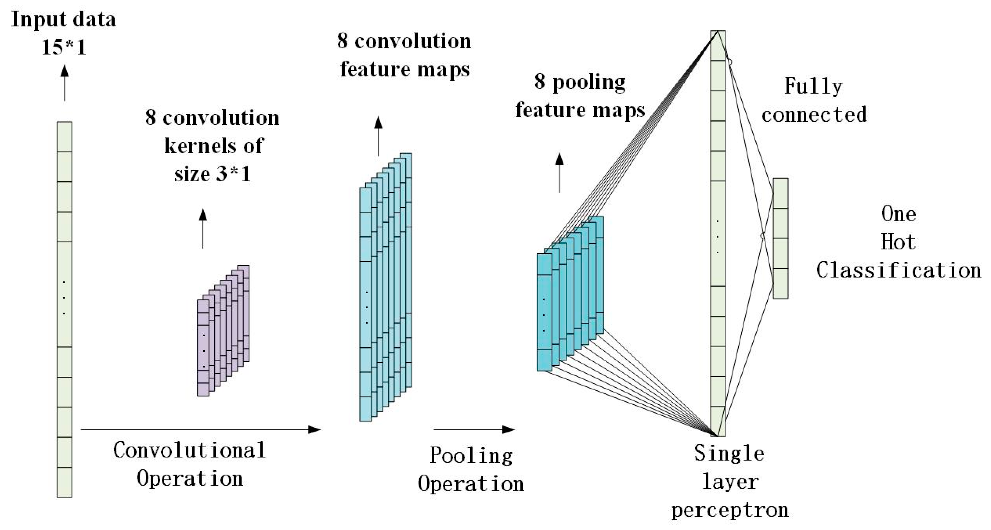
As a feedforward neural network, one-dimensional neural network (1D-CNN) is inspired by the mammalian visual cortex receptive field. The network perceives the local features and integrates the local features in high-dimensional space, and finally obtains global information. The basic structure of the convolutional neural network includes an input layer, alternating convolution layers, pooling layers, and a fully connected layer. The convolutional layer captures the information of the local connections in the input features through the convolution kernel and reduces the parameters of the model using the weight sharing principle. The convolution formula is:
where represents the transfer function, represents the j-th feature map of convolutional layer l, M represents the number of feature maps, represents the ith feature map of the l-1 layer, represents convolution operation, represents trainable convolution kernel, and represents bias. The shape and number of one-dimensional convolution kernels can largely determine the feature-extraction ability of the overall network. The shape of the convolution kernel affects the fineness of feature extraction. The number of convolution kernels corresponds to the size of the feature layer, affecting multiple ways of feature extraction and the computational scale of the network. The pooling layer combines multiple adjacent nodes to merge similar features and performs down-sampling operation on the feature layer extracted by the convolutional layer, thereby reducing training parameters and preventing network over-fitting to enhance the generalization ability of the network. At present, the main pooling methods include maximum pooling, mean pooling, and L2-norm pooling. After the convolutional layer and pooling layer are located, the fully connected layer trains the weights and biases of the convolution kernels in the entire convolutional neural network based on the back-propagation principle. The fully connected layer structure is similar to the BP neural network mentioned in the previous section, which has a hidden layer and uses the Softmax activation function to complete the classification. The structure of the entire network is shown in Figure 5.
2.2.4. Decision Tree
DT is a common machine learning algorithm similar to the tree structure, often used to find pattern structures in data. It aims to establish correct decision rules and determine the relationship between feature attributes and target variables without expert experience. Usually DT contains a root node, multiple internal nodes, and a set of leaf nodes from top to bottom. The leaf node corresponds to the prediction result, and the node contains all samples. The key to DT learning is to divide the best attributes. At present, the algorithms for constructing DT mainly include CART, C4.5 and ID3. This study uses a CART algorithm with better performance and efficiency [38]. CART uses the Gini coefficient to divide the node properties and establish a DT by selecting the attributes that minimize the Gini coefficient after dividing the nodes. The Gini index is shown in Equation (5) where k is the category and t is the node. Finally, pruning techniques are used to deal with the over-fitting problem of the model. Upon completing the entire algorithm, we can clearly understand the internal decision-making mechanism and thus get a more objective knowledge of debris flow triggering factors.
2.2.5. Random Forest
As an integrated classification algorithm of machine learning, RF aims to improve the flexibility and accuracy of classification trees. In RF, a large number of trees are generated by constructing a base DT on multiple bootstrap sample sets of data during the running of the algorithm. Because the feature attributes of each node are randomly selected, the node characteristics are effectively reduced without increasing the deviation. Each feature subset is much smaller than the total number of features in the input space so that each DT is decorrelated. Finally, the output of the classification task is predicted by a simple voting method. RF has been constructed with a number of DTs. It has been greatly improved compared with a single DT. However, RF is as complex as the single basic DT. Therefore, RF is also a fairly effective integrated learning algorithm.
2.2.6. XGBoost
XGBoost, also known as extreme Gradient Boosting, is a gradient-enhanced integration algorithm based on classification trees or regression trees. It works the same way as Gradient Boosting, but adds features similar to Adaboost. The algorithm combines multiple DT models in an iterative way to form a classification model with a better structure and higher precision. It has achieved impressive results in many international data mining competitions and won more than two championships in the Kaggle competition. In the DFS analysis experiment, the XGBoost can classify the DFS level according to the environmental characteristics of the Shigatse region and rank the importance of the triggering factors.
The XGBoost uses both the first and second derivatives to perform Taylor expansion on the loss function and adds a regular term to it. Therefore, while considering the model accuracy, the model complexity is also well controlled. Finally, the predictive power of the model is trained by minimizing the total loss function [39]. The objective function of the model can be expressed as Equation (6):
where i represents the ith sample, represents the predicted value of the (t − 1)th model for the sample i, represents the newly added tth model, represents the regular term, C represents some constant terms, and the outermost L() represents the error.
The optimizer aims to calculate the structure and the leaf score of the CART tree. XGBoost accelerates existing lifting tree enhancement algorithms through the cache-aware read-ahead technology, distributed external memory computing technology and AllReduce fault-tolerant tools. It can also be trained by using a graphics processing unit to provide a very high speed boost.
In this work, we can import the XGBoost toolkit in Python. The training process controls the establishment of DT by adjusting five hyper-parameters: the number of iterations, the number of trees generated, the learning rate, the maximum depth of each tree, and the L2 regularization. The Gamma hyper-parameter limits the gain amount required for segmentation.
2.3. Evaluation Measures
DFS mapping should have the ability to effectively predict the probability of future debris flows in the study area. In order to evaluate the predictive power of several machine learning algorithms, five common evaluation methods are used to quantify model performances, including Precision, Recall, F1 score, Accuracy and AUC. Finally, 293 debris flow events are applied as a test set.
In the case of the binary classification problem, four elements, i.e., TP, TN, FP and FN, are defined as follows.
TP: True Positive. Samples belonging to the TRUE class are correctly marked as positive by the model.
TN: True Negative. Samples belonging to the TRUE class are incorrectly marked as negative by the model.
FP: False Positive. Samples belonging to the FALSE class are incorrectly marked as positive by the model.
FN: False Negative. Samples belonging to the FALSE class are correctly marked as negative by the model.
2.3.1. Precision
In the binary classification task, precision represents the ratio of the correct labeled True class samples to the total number of predicted values labeled true. The formula is as follows:
Precision = TP/(TP + FP)
Precision is expressed as a weighted average of the precision of each class in a multivariate classification task.
2.3.2. Recall
The Recall rate is the ratio of the correct labeled True sample to the total number of True samples, expressed as Equation (8) in the binary classification task.
Recall = TP/(TP + FN)
The Recall rate represents the weighted average of the Recall rates for each category in a multivariate classification task.
2.3.3. F1 Score
The F1 score is represented by Precision and Recall, with values between 0 and 1, which represent the worst and best, respectively. The relative contributions of accuracy and recall to the F1 score are equal. The formula is defined as follows:
F1 score = 2 * (Precision * Recall)/(Precision + Recall)
In a multivariate classification task, the F1 score represents a weighted average of F1 scores for each category.
2.3.4. Accuracy
In a multivariate classification task, accuracy represents the ratio of correctly classified samples to the total number of samples.
2.3.5. Area Under the Curve (AUC)
The AUC method is defined as the area under the receiver operating characteristic curve (ROC), which can give different distributions of each class. It can be used to judge classifiers’ performance. The ROC curve is plotted as the relationship between the true positive rate (TPR) and false positive rate (FPR). TPR represents the ratio of the positive instance correctly classified to the total number of all the positive instances, as represented by Equation (10):
TPR = TP/(TP+ FN)
FPR is the ratio of the positive instance misclassified to the total number of all the negative instances, as represented by Equation (11):
FPR = FP/(FP + TN)
The AUC method is also designed to evaluate the binary classification. First, we need to convert the multivariate classification task into multiple binary classification, and then separately calculate the AUC values of the respective categories. Finally, the multivariate classification result is obtained by obtaining the average of the total AUC values [40].
2.4. Cross-Validation
In this paper, the cross-validation method is used to complete the parameter optimization. Specifically, based on the error-based verification evaluation index, the training set is divided into k pairs of mutually equal exclusion subsets, where k − 1 pairs are used as the training sets and the remaining subset are used as the verification set. The experiment is performed by rotating the subset k times in turn, and the k verification results are averaged. In this paper, the GridSearchCV module via the scikit-learn and the cv function via the XGBoost library are used to optimize the parameters of the decision tree, random forest and the XGBoost model. In the Keras framework, the cross-validation method based on the GridSearchCV module is also used to search in the parameter space, and the optimal parameter estimation of the model in the data set is given.
2.5. Statistical Analysis
In order to compare the performance differences between the models, we conducted a statistical analysis. One-way ANOVA can be used to test whether there is a statistically significant difference in two or more unrelated groups [41]. Model performance is evaluated by the accuracy of test results during the model training. Therefore, the accuracy group obtained by cross-validation of different algorithms is used for one-way ANOVA. The null hypothesis given by H0 tested by One-way ANOVA is as follows.
H0: The accuracy of all algorithms is not significantly different.
H1: There are significant differences in the accuracy of at least two or more algorithms.
The One-way ANOVA results in a P-value, and the P-value is the risk of rejecting the hypothesis H0.
The results can only determine whether there is a significant difference between at least one group of samples and other groups, but it is impossible to judge whether there is a difference between the two groups. Therefore, comparisons between specific groups are often performed after one-way ANOVA. The honestly significant difference (HSD) method was developed by Tukey and is favored by researchers as a simple and practical pairwise comparison technique. The main idea of HSD is to use the statistical distribution to calculate the true significant difference between two mean values and call it q-distribution [42]. This distribution gives an exact sampling distribution of the largest difference between a set of mean values in the same population. All pairwise differences were evaluated by using this distribution. This paper uses HSD as a post-hoc analysis to test the variance homogeneity of performance indicators from different algorithms.
All statistical analyses were completed by using the Statistical Package for Social Sciences (IBM SPSS Statistics for Windows Version 22.0).
2.6. Feature Importance
The tree-based machine learning approach in this study provides a “feature importance” toolkit for ordering index factors based on the function strength of a particular problem [43]. In the basic decision tree, feature attributes are selected for the node segmentation, and the number of times measures the importance of the attribute. For a single decision tree T, Equation (12) represents the score of importance for each predictor feature , and the decision tree has J − 1 internal nodes.
The selected feature is the one that provides maximal estimated improvement in the squared error risk over that for a constant fit over the entire region. The following formula represents the importance calculation over the additive M trees.
In reality, a frequently used attribute often has a good distinguishing ability. In this study, the importance of the factors affecting the debris flows occurrences is ranked from high to low according to the characteristic attribute of the decision-making process of DFS.
3. Results
In this section, a specific implementation of five machine learning algorithms is introduced. Using Python as the development language, the BPNN and the 1D-CNN are constructed based on the Keras learning framework. The DT and the RF are implemented by API provided by the scikit-learn module, and the XGBoost algorithm is implemented by the Python-based code provided by its official website. The performance of DFS model depends largely on the choice, adjustment and optimization of its parameters. Therefore, the optimization of the model structure and parameters requires multiple experiments. The cross-validation method is used to complete the parameter optimization. After many experiments, the optimal parameters of the five DFS models are obtained as shown in Table 3.
3.1. Performance Metrics Evaluation
Cross-validation produces a list of accuracy, which can be seen from the first row in Table 4. The poor accuracy value in the second line indicates the performance of the model under the non-SMOTE data set.
In order to obtain robust verification results, we use the One-way ANOVA method to test whether there is a significant difference between the methods. The ANOVA method is used according to the five groups of accuracy, and the results are shown in Table 5.
The F value in the table indicates the ratio of the mean square between the groups to the mean square within the group. The corresponding P value is found according to the F value through the lookup table. Sig represents the P value, which is 0 and less than 0.05, indicating that we can reject the null hypothesis H0. We can think that there are significant differences between at least two sets of models. Significant differences are calculated according to post-hoc Tukey’s HSD for all pairwise comparisons between accuracies as shown in Table 6.
According to statistics, XGBoost performs best in terms of accuracy, and there is a significant difference (p < 0.005) from BPNN, DT and RF. There is no significant difference between XGBoost and CNN, but the average accuracy of XGBoost is higher than that of 1D-CNN.
3.2. DFS Map Construction
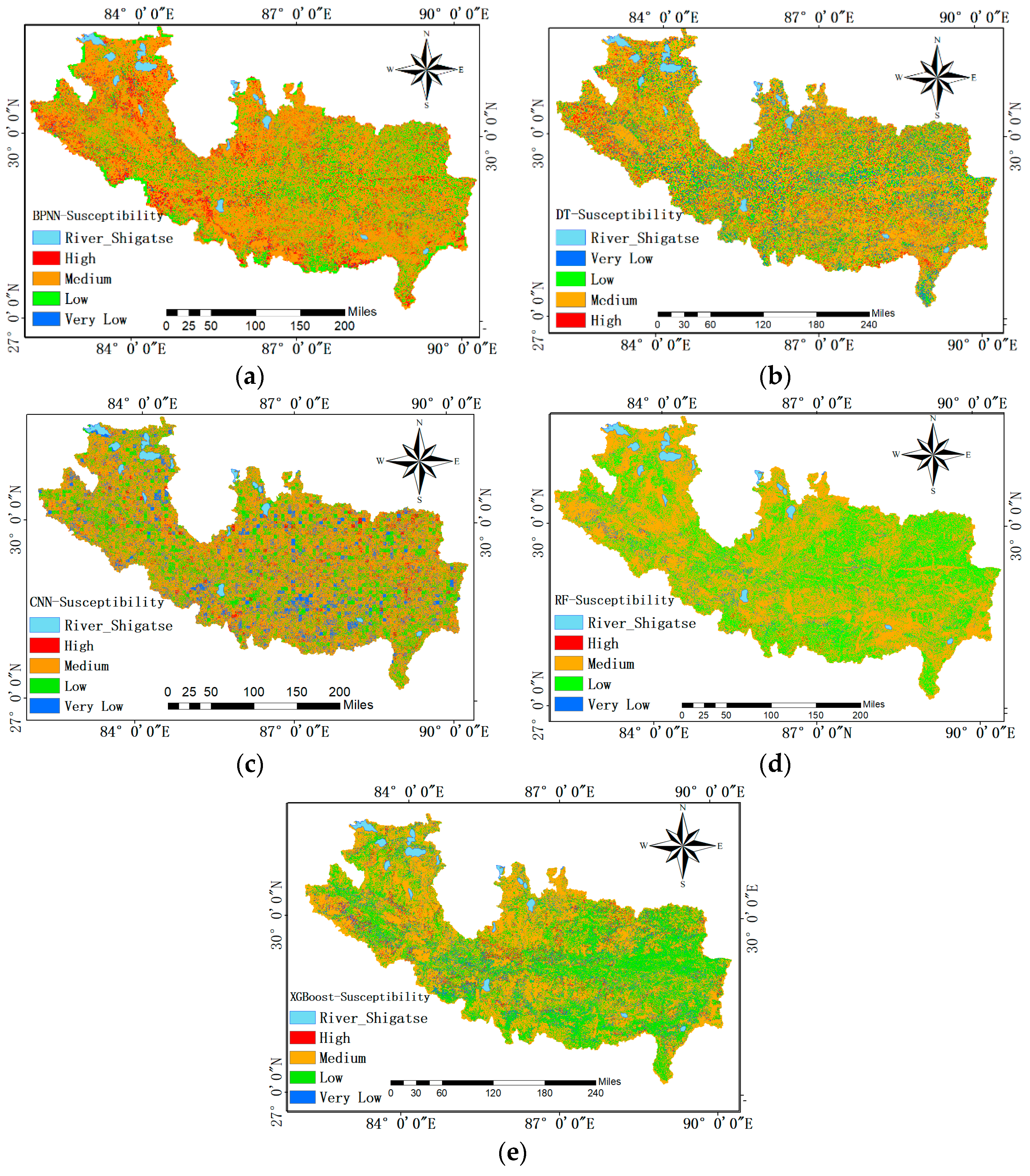
In this study, the relationships between the debris flow triggering factors and the DFS levels are fitted by training the BPNN, CNN, DT, RF and XGBoost models to predict the susceptibility index of each pixel in the study area, and to establish a pixel-based DFS classification map (Figure 6). The result is a raster map with each raster pixel assigned a unique susceptibility index value. The susceptibility index values are divided into four categories: 0, 1, 2 and 3, indicating very low, low, medium and high debris flow levels, respectively.
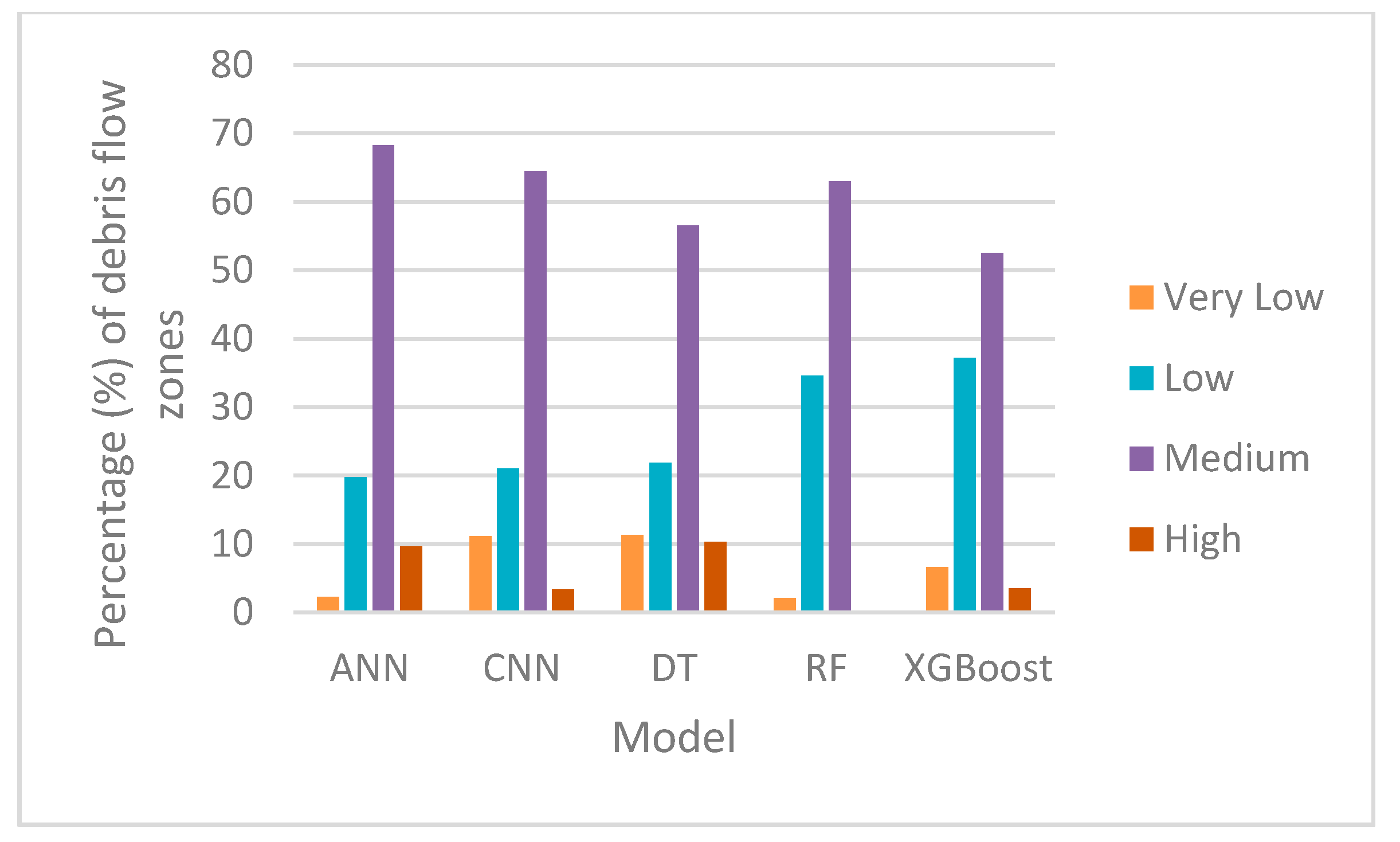
In the debris flow map constructed by the BPNN model, about 2% of the study area is not susceptible to debris flow, and the other 19.8%, 68.1%, and 9.6% are low, medium and high probability DFS levels, respectively, as shown in Figure 6a.
The debris flow susceptibility map predicted by 1D-CNN is shown in Figure 6c. Among them, the medium-prone area accounts for the vast majority of the study area. The other 11.12%, 21.02% and 3.35% are very low, Low and high probability DFS levels, respectively.
The DFS map generated by the DT model is shown in Figure 6b. 11.2% of the study area is not susceptible to debris flows, 21.8% is seldom affected by debris flows, while the medium probability debris flow area accounts for 56.5%, and the remaining 10.3% is high-probability area (Figure 6b).
The proportion of each RF susceptibility level in the DFS map fitted by the RF model is very low (2.1%), low (34.5%), medium (62.8%), and high (0.27%), as shown in Figure 6d.
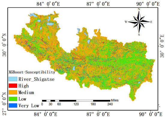
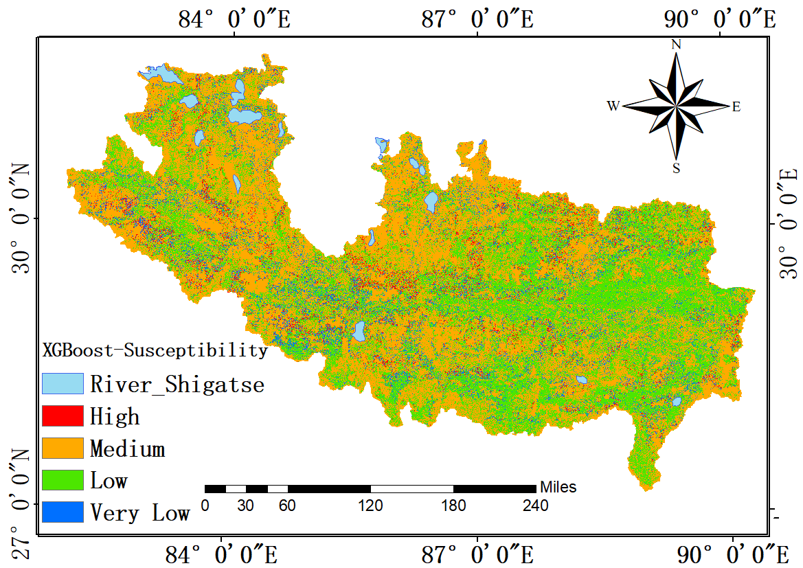
Finally, based on the XGBoost model, a DFS map is generated as shown in Figure 6e. The results of DFS level distribution are very similar to those based on the random forest model. The medium susceptibility is the main debris flow level, which accounts for 52.5%; the second large area corresponds to the low susceptibility level, 37.2%. Very low and highly susceptible areas are small, accounting for 6.6% and 3%, respectively (Figure 7).
3.3. Model Evaluation
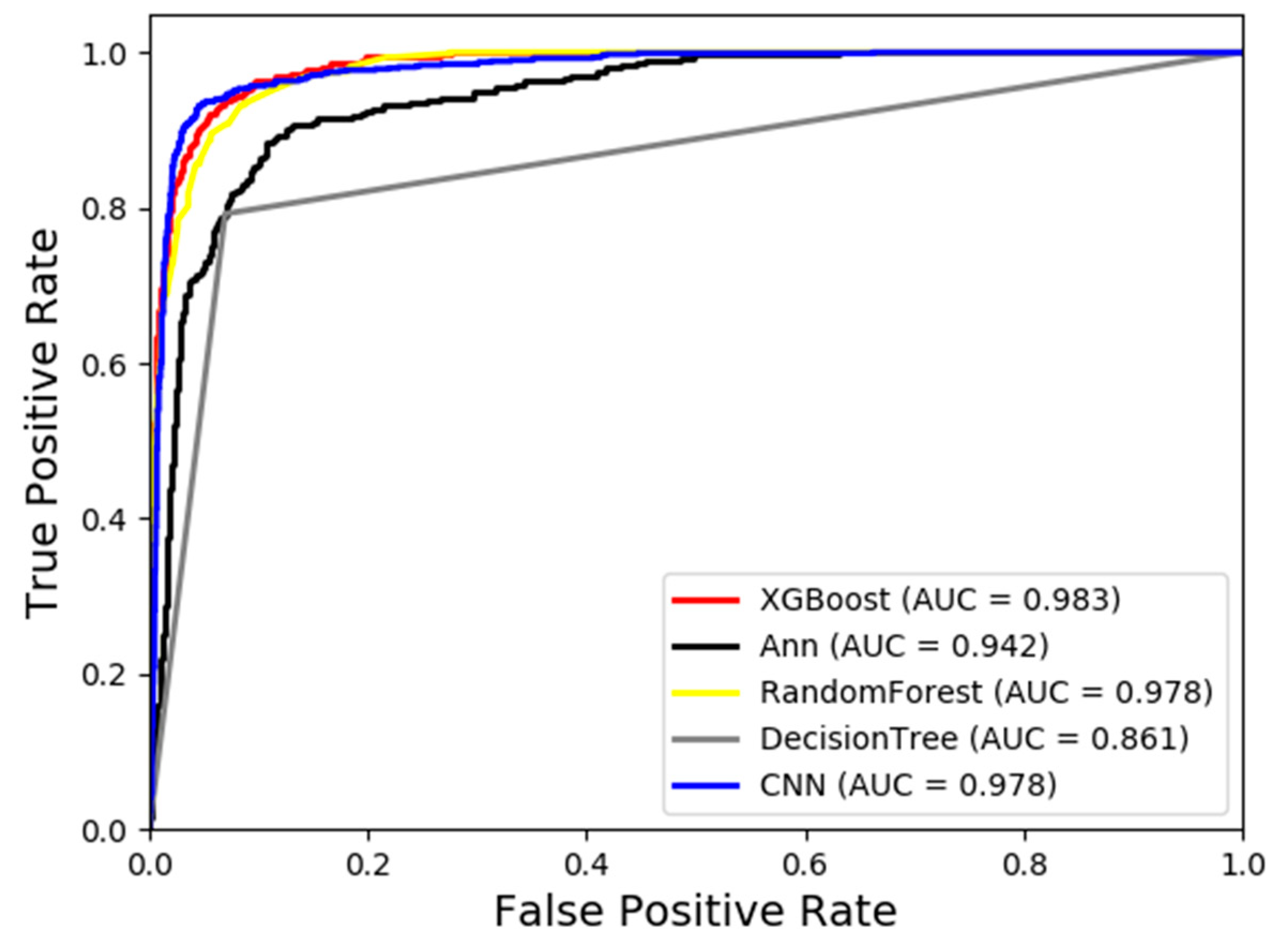
After successfully constructing the DFS model, we evaluated its performance using five traditional evaluation methods, i.e., Recall, Precision, F1 score, Accuracy, and AUC. We also calculated the time required to forecast the entire study area. The results of each model are shown in Table 7. In particular, because the ROC curve corresponding to the AUC index of each model can directly reflect the advantages and disadvantages of the model, it is drawn in Figure 8. As seen from Table 7 and Figure 8, the following findings are listed.
- (1)
- The values of the Recall, Precision, F1 score, Accuracy, and AUC evaluation score of the five algorithms are quite different. That is, the performances of different algorithms show great differences in the test set.
- (2)
- Despite large differences in the evaluation index values, their differences show the same trend. That is, the algorithm is superior when each evaluation index is superior to the other algorithms.
- (3)
- The AUC evaluation scores of the five algorithms are very high, indicating that they are excellent for evaluating the DFS in our study area. The AUC values of the BPNN, 1D-CNN, DT, RF and XGBoost are 0.946, 0.976, 0.911, 0.976 and 0.988, respectively. It can be seen that XGBoost has the best performance.
- (4)
- From the results of the five indicators, the evaluation scores of the BPNN and DT models are similar, and the 1D-CNN, RF and XGBoost models also take approximate scores, but the former has a large gap with the latter.
- (5)
- The models in this manuscript are all operated on Intel (R) Core (TM) i7-6800K CPU @ 3.4 GHz with 64 RAM servers. In terms of predicting the time of the entire area, the DT model takes the shortest time. XGBoost and 1D-CNN models take about the same time, and the calculation time is at a medium level. The prediction speed of the BPNN model is slow, which takes about 20 min for a single prediction. Finally, it can be seen that the RF calculation takes the longest time.
3.4. Importance of Triggering Factors
After successfully implementing the five evaluation algorithms, it is concluded that the XGBoost model performs the best in the DFS mapping, and the model can be used to fit the relationship between the debris flow triggering factors and the susceptibility. However, not all selected debris flow triggering factors have a good predictive power. Different triggering factors have different contributions to the model. Therefore, it is necessary to understand the contribution of each triggering factor. The practical significance of this research is that we can provide suggestions and references for local governments and researchers on site selection for public facilities by studying the importance of different debris flow triggering factors characteristics.
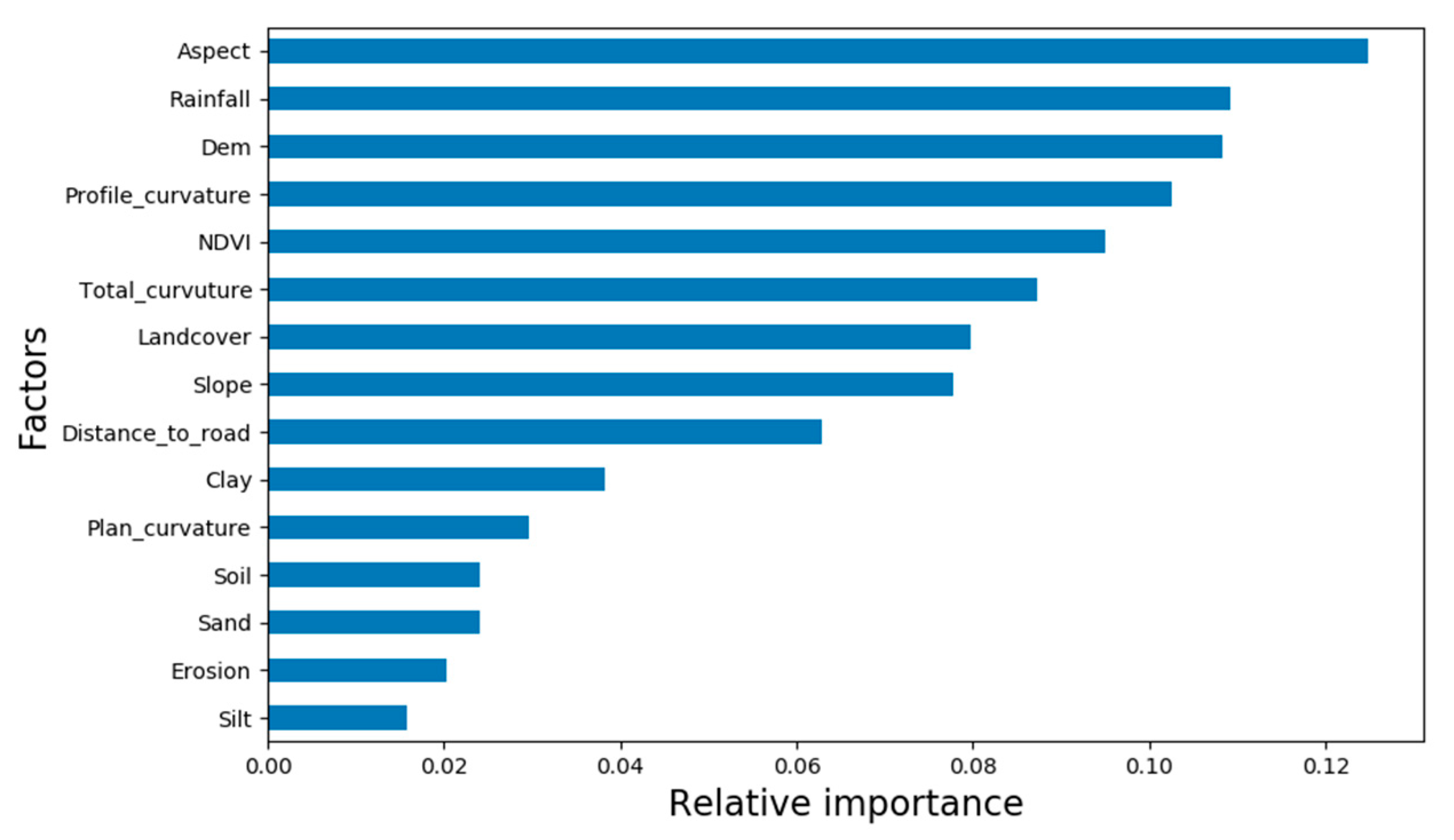
As shown in Figure 9, the ordinate represents fifteen index factors for evaluating the DFS, and the abscissa is expressed as the ratio of the number of times each feature attribute used for DT node segmentation to that all attributes used for node segmentation. It can be clearly seen that the aspect is the most important factor affecting the occurrence of debris flows, closely followed by the rainfall, and the impacts of elevation and slope curvature are ranked the third and fourth, respectively. According to these main characteristics, topographic and climatic factors are the main triggering factors for the occurrence of debris flows in Shigatse. The last few debris flow triggering factors ranked by feature importance have relatively little impact on debris flow events especially soil factors.
4. Discussion
This study aims to estimate the regional DFS by using five highly representative machine learning models, i.e., BPNN, 1D-CNN, DT, RF, and XGBoost. According to literature, such investigations are rare in Shigatse, particularly based on 1D-CNN and XGBoost.
4.1. Model Performance
First, as seen from Table 4, category imbalances have caused over-fitting problems on all of the above machine learning models, resulting in poor model performance. The data generated by the interpolation method is close to the original data, and we will adopt better interpolation methods to obtain more reasonable data and use other methods to alleviate the over-fitting problem of machine learning for unbalanced data [44] in the future studies.
As shown in Table 7, among the five evaluation methods (Recall, Precision, F1 score, Accuracy and AUC), the results show that there is a gap in performance among different algorithms. The performance rankings of the five models from high to low are XGBoost, 1D-CNN, RF, BPNN and DT. In addition, ANOVA and Tukey HSD test results show that XGBoost is significantly different from the RF, BPNN, and DT models. This also shows that XGBoost’s generalization performance and predictive ability are significantly better than RF, BPNN and DT.
In the early days, BPNN showed excellent performance in a variety of classification tasks. However, this research only demonstrates its accuracy to outperform a single DT. XGBoost is not only better than BPNN in terms of accuracy, but also in terms of speed, because BPNN has too many parameters to be adjusted. Especially, XGBoost can generate “feature importance” that allows researchers to analyze the data and BPNN is a black box model, for which much research has been done to explain the internal structure. Although XGBoost has not been used for debris flow susceptibility analysis, some scholars in the field of mountain disaster study have similar conclusions that the boost model exceeds the accuracy of BPNN by 8% [18].
RF and XGBoost are integrated machine learning algorithms based on DT. The corresponding evaluation scores are higher than that of a single DT. Such a result shows that the integrated algorithm can make up the lack of fitting ability of a single DT. Although RF and XGBoost are both integrated machine learning algorithms, XGBoost’s overall performance is better than the RF algorithm. The RF algorithm focuses on the final voting results of all DTs, which can reduce variance, while XGBoost focuses on the residuals generated by the last iteration which can reduce both variance and bias. Performance comparisons between XGBoost and RF have been commonly obtained in many research areas. Usually, XGBoost is in the leading position [39,45].
Like XGoost, 1D-CNN has not been used in debris flow susceptibility, and little literature is concerned about them. The cross-validation results show that the accuracies of XGBoost and 1D-CNN are not significantly different, but the average accuracy of XGBoost is better than that of 1D-CNN. The test performance of the two models is also led by XGBoost. The main reason for this result is that CNN can capture things like image, audio and possibly text quite well by modeling the spatial temporal locality, while tree-based models solve tabular data very well.
When considering the model classification performance comprehensively, we can find that XGBoost has the best comprehensive performance with high classification accuracy, good prediction effect and less calculation time. Therefore, the XGBoost research method should attract more attention in the future evaluation of DFS.
4.2. Feature Importance
Based on the selected model to construct the DFS map, the following conclusions can be drawn from Figure 4. The DFS in the study area is mainly medium and low, accounting for more than 50% of the entire study area. The feature attribute scores provided by the tree-based machine learning method are important for analyzing the cause of debris flows. The results have shown that the aspect, profile curvature, annual average rainfall and DEM are the main factors affecting the occurrence of debris flows in the study area. The other triggering factors such as vegetation cover and human activities also have a certain impact on debris flow, while the contribution of soil factors to the modeling is relatively weak. According to the evaluation results of the model feature attributes, the targeted analysis and investigation of the debris flow triggering factors in the study area can be carried out. Based on historical data statistics, analysis of the main triggering factors is conducted.
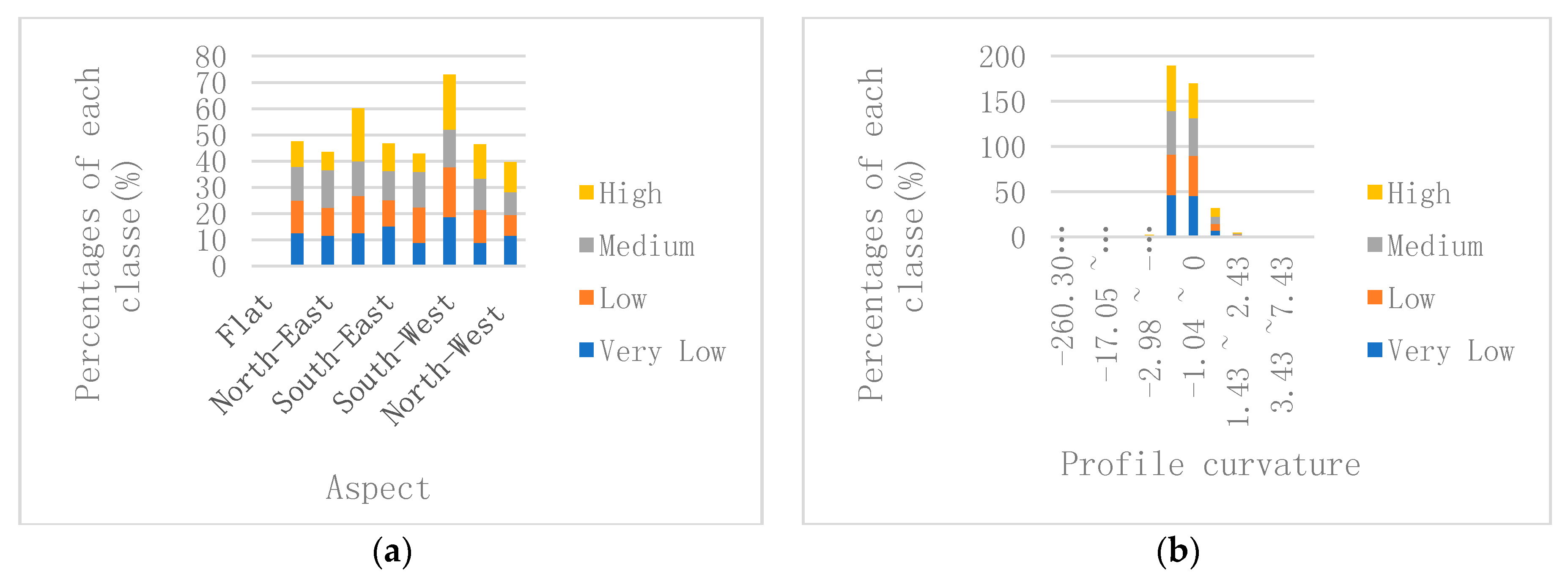
In the study area, different slope directions lead to differences in hydrothermal conditions, which in turn affect the geographical element distributions such as vegetation, hydrology, soil, and topography. Some Chinese scholars have also examined the relationship between vegetation and debris flow erosion and suggested that the slope direction largely determines the vegetation type and soil type [46]. Feature selection show that the slope aspect has the greatest impact on the distribution of debris flows. According to the actual debris flow events statistics (Figure 10a), the distribution of debris flow events in each aspect is given, and the number of debris flows on the southwest slope and the east slope are relatively large. Among them, the debris flow events on the southwest slope are the densest as well as the distribution location of highly occurrence-prone debris flow events.
The curvature of the slope describes its shape, which controls the formation of debris flow events by affecting the gravitational potential energy and water collection conditions. The feature selection results show that the profile curvature can be better used to estimate the DFS than the plane curvature and total curvature. The shape of the slope is usually linear, concave or convex, indicating the mid-term evolution of the landscape, the maturity of the landscape and the period of violence of the landscape, respectively. According to the statistic (Figure 10b), the debris flows are mainly concentrated in the area where the curvature is negative, i.e., the surface of the pixel is convex. This statistical result is consistent with the results of Guo et al. [47] on mountain debris flow events.
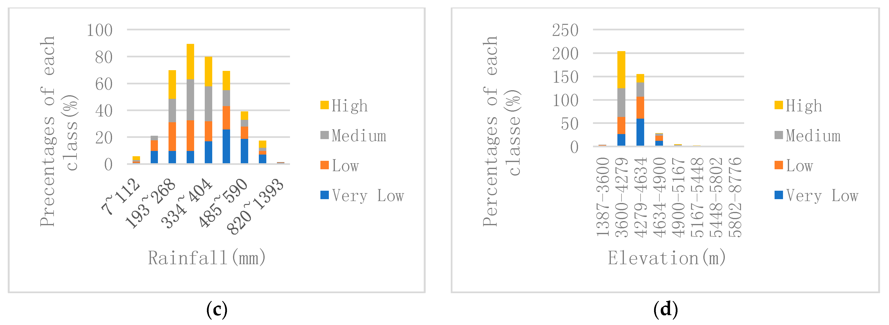
The overall elevation of the Shigatse region is very high and the valley is deep. Statistics on the distribution of debris flow events at different altitudes indicate that debris flow events are mainly distributed at altitudes between 3600–4600 m (Figure 10c). High-susceptibility and medium-susceptibility levels are distributed at the altitude of about 4000 m. The reason is that the region at the altitude between 3600 and 4600 m is very steep and densely populated. As a result, human activities have a huge impact on it. In addition, the area within this altitude is mainly eroded by flowing water with serious accumulation of loose materials and debris flow events particularly develop. Tang et al. [31] also got similar conclusions for the investigation of the study area.
Rainfall is the main triggering factor for debris flows. It mainly promotes the mountain debris flows by increasing soil bulk density and reducing cohesion and internal friction. The study area is mainly a rain-sparing region with annual average rainfall less than 1350 mm (Figure 10d). However, the debris flow has a very significant correlation with the rainfall season in Shigatse. Although the annual precipitation is not high, the temporal distribution is concentrated. That is, heavy rain season is also the season when debris flows frequently occur. According to statistics, debris flows in the flood season in Shigatse accounts for more than 70% of the total debris flows.
Machine learning algorithms can handle large-scale data. In addition, they are more objective than the traditional qualitative evaluation methods and can support making decisions without expert system support. However, there are some inherent problems. For example, the data preprocessing workload is large and time-consuming, and the data processing results have a great impact on the classifier.
5. Conclusions
In this study, multi-source satellite data and GIS are used to characterize the gestation environment of debris flows in the study area, and then input these environmental characteristics into the machine learning methods to establish the DFS model. The role and weight of the triggering factors shown by the training process are analyzed for the purpose of further studying the main causes of debris flow. In the entire research process described above, the four main findings are described as follows:
- (1)
- Satellite remote sensing can provide data for regional DFS analysis, especially for mountainous areas such as the southwestern Tibet with steep terrain where the sites are not always accessible for investigation. Higher resolution does allow the image to better describe the terrain where the debris flow occurs [48] and potentially improve further analysis. It is important and necessary to use topographical factors, human activities, vegetation cover, climatic and soil elements provided by satellite remote sensing to estimate regional debris flow susceptibility.
- (2)
- Five machine learning algorithms were used to construct DFS map in Shigatse. The results confirm that all five methods can be used to analyze the susceptibility of debris flows. According to the performance, XGBoost ranks the first, and 1D-CNN is the second, followed by RF, BPNN, and DT. XGBoost has the best predictive performance with the highest score among the five evaluation methods. The ANOVA method and the Tukey’s HSD test showed that the accuracy of XGBoost is significantly better than those of RF, BPNN, and DT, but it is not significantly different from 1D-CNN. In terms of the time required for prediction, DT takes the least time, and the time required for 1D-CNN is moderate and close to XGBoost. RF and BPNN are slower to calculate. It is notable that this is the first comparative experiment of XGBoost and 1D-CNN in the study of DFS. The ranking of the model based on the “feature importance” indicates that the slope aspect, rainfall, profile curvature and DEM have a greater impact on the debris flows. The results of this study are significant for the local public facility construction and the residential property protection. Therefore, the XGBoost method has good prospects in estimating the DFS.
- (3)
- By comparing the debris flow susceptibility maps of the five prediction algorithms, it is found that the prediction results of five models all show that the moderately susceptible areas account for a large proportion. This experiment has not yet explained the reasons for the different prediction results. The causes will be explored in the subsequent studies. There may be some shortcomings in the use of susceptibility in statistics as a label in experiments. In the follow-up study, we are going to use the clustering algorithm first to obtain the location where the debris flow is not easy to occur and use it together with the existing debris flow data for the classification of debris flow susceptibility. With the development of machine learning technology, we will strive to further improve the performance of the model for DFS by modifying and optimizing the algorithm.
- (4)
- Debris flows are common in mountain areas. Five machine learning models are used to analyze the debris flow events in the study. The results show that the XGBoost model has the best predictive performance, which can be used to prevent casualties and economic losses caused by debris flows. For local land planning and land use, relevant departments can use the XGBoost model in combination with satellite remote sensing and GIS spatial data processing to create feature maps and high-precision area-sensitive maps to provide guidance and preparation for debris flow prevention and mitigation.
Author Contributions
Conceptualization, Y.Z. and T.G.; methodology, T.G.; software, T.G.; validation, W.T., and Y.Z.; formal analysis, T.G.; investigation, T.G.; resources, Y.Z.; data curation, W.T.; writing—original draft preparation, T.G.; writing—review and editing, Y.Z., W.T., Y.-A.L.; visualization, T.G.; supervision, W.T.; project administration, Y.Z.; funding acquisition, Y.Z.
Funding
This research was funded by the National Natural Science Foundation of China, grant number 41661144039, 41875027 and 41871238.
Acknowledgments
The authors would like to thank the Tibet Plateau Institute of Atmospheric Environment, Geospatial data cloud, Resource and Environmental Cloud Platform, earth observing system data and information system and Geoscientific Data & Discovery Publishing Systems for the data that they kindly provided. Acknowledgement for the data support from “National Earth System Science Data Sharing Infrastructure, National Science & Technology Infrastructure of China. (http://www.geodata.cn)”.
Conflicts of Interest
The authors declare no conflict of interest.
References
- Iverson, R.M. Debris-flow mechanics. In Debris-Flow Hazards and Related Phenomena; Springer: Berlin/Heidelberg, Germany, 2005; pp. 105–134. ISBN 9783540207269. [Google Scholar]
- Golovko, D.; Roessner, S.; Behling, R.; Wetzel, H.U.; Kleinschmit, B. Evaluation of remote-sensing-based landslide inventories for hazard assessment in Southern Kyrgyzstan. Remote Sens. 2017, 9, 943. [Google Scholar] [CrossRef]
- LV, X.; Ding, M.; Zhang, Y.; Teng, J. Hazard assessment of mountainous disasters in Nieyou section of Sino-Nepal highway based on triangle whitening weight function. J. Southwest Univ. Sci. Technol. 2017, 1. [Google Scholar] [CrossRef]
- Sun, Y.; Chen, H.; Zhang, Z.; Zhao, Y.; Bao, P.; Bai, J. Distribution regularities of geological hazards along the g318 lhasa-shigatse section and their influence factors. J. Nat. Disasters 2014, 23, 111–119. [Google Scholar]
- Gregoretti, C.; Stancanelli, L.M.; Bernard, M.; Boreggio, M.; Degetto, M.; Lanzoni, S. Relevance of erosion processes when modelling in-channel gravel debris flows for efficient hazard assessment. J. Hydrol. 2019, 568, 575–591. [Google Scholar] [CrossRef]
- Kim, H.; Lee, S.W.; Yune, C.Y.; Kim, G. Volume estimation of small scale debris flows based on observations of topographic changes using airborne LiDAR DEMs. J. Mt. Sci. 2014, 11, 578–591. [Google Scholar] [CrossRef]
- Kim, H.S.; Chung, C.K.; Kim, S.R.; Kim, K.S. A GIS-based framework for real-time debris-flow hazard assessment for expressways in Korea. Int. J. Disaster Risk Sci. 2016, 7, 293–311. [Google Scholar] [CrossRef]
- Alharbi, T.; Sultan, M.; Sefry, S.; ElKadiri, R.; Ahmed, M.; Chase, R.; Chounaird, K. An assessment of landslide susceptibility in the Faifa area, Saudi Arabia, using remote sensing and GIS techniques. Nat. Hazards Earth Syst. Sci. 2014, 14, 1553. [Google Scholar] [CrossRef]
- Ahmed, B.; Dewan, A. Application of bivariate and multivariate statistical techniques in landslide susceptibility modeling in Chittagong City Corporation, Bangladesh. Remote Sens. 2017, 9, 304. [Google Scholar] [CrossRef]
- Li, Y.; Wang, H.; Chen, J.; Shang, Y. Debris flow susceptibility assessment in the Wudongde Dam area, China based on rock engineering system and fuzzy C-means algorithm. Water 2017, 9, 669. [Google Scholar] [CrossRef]
- Liou, Y.A.; Nguyen, A.K.; Li, M.H. Assessing spatiotemporal eco-environmental vulnerability by Landsat data. Ecol. Indic. 2017, 80, 52–65. [Google Scholar] [CrossRef]
- Sujatha, E.R.; Sridhar, V. Mapping debris flow susceptibility using analytical network process in Kodaikkanal Hills, Tamil Nadu (India). J. Earth Syst. Sci. 2017, 126, 116. [Google Scholar] [CrossRef]
- Aditian, A.; Kubota, T.; Shinohara, Y. Comparison of GIS-based landslide susceptibility models using frequency ratio, logistic regression, and artificial neural network in a tertiary region of Ambon, Indonesia. Geomorphology 2018, 318, 101–111. [Google Scholar] [CrossRef]
- Di Cristo, C.; Iervolino, M.; Vacca, A. Applicability of Kinematic and Diffusive models for mud-flows: A steady state analysis. J. Hydrol. 2018, 559, 585–595. [Google Scholar] [CrossRef]
- Xu, W.B.; Yu, W.J.; Jing, S.C.; Zhang, G.P.; Huang, J.X. Debris flow susceptibility assessment by GIS and information value model in a large-scale region, Sichuan Province (China). Nat. Hazards 2013, 65, 1379–1392. [Google Scholar] [CrossRef]
- Chen, X.; Chen, H.; You, Y.; Chen, X.; Liu, J. Weights-of-evidence method based on GIS for assessing susceptibility to debris flows in Kangding County, Sichuan Province, China. Environ. Earth Sci. 2016, 75, 70. [Google Scholar] [CrossRef]
- Achour, Y.; Garçia, S.; Cavaleiro, V. GIS-based spatial prediction of debris flows using logistic regression and frequency ratio models for Zêzere River basin and its surrounding area, Northwest Covilhã, Portugal. Arab. J. Geosci. 2018, 11, 550. [Google Scholar] [CrossRef]
- Oh, H.J.; Lee, S. Shallow landslide susceptibility modeling using the sata mining models artificial neural network and boosted tree. Appl. Sci. 2017, 7, 1000. [Google Scholar] [CrossRef]
- Shirzadi, A.; Shahabi, H.; Chapi, K.; Bui, D.T.; Pham, B.T.; Shahedi, K.; Ahmad, B.B. A comparative study between popular statistical and machine learning methods for simulating volume of landslides. Catena 2017, 157, 213–226. [Google Scholar] [CrossRef]
- Wang, L.J.; Guo, M.; Sawada, K.; Lin, J.; Zhang, J. A comparative study of landslide susceptibility maps using logistic regression, frequency ratio, decision tree, weights of evidence and artificial neural network. Geosci. J. 2016, 20, 117–136. [Google Scholar] [CrossRef]
- Abancó, C.; Hürlimann, M. Estimate of the debris-flow entrainment using field and topographical data. Nat. Hazards 2014, 71, 363–383. [Google Scholar] [CrossRef]
- Prenner, D.; Kaitna, R.; Mostbauer, K.; Hrachowitz, M. The value of using multiple hydrometeorological variables to predict temporal debris flow susceptibility in an alpine environment. Water Resour. Res. 2018, 54, 6822–6843. [Google Scholar] [CrossRef]
- Jiang, W.; Rao, P.; Cao, R.; Tang, Z.; Chen, K. Comparative evaluation of geological disaster susceptibility using multi-regression methods and spatial accuracy validation. J. Geogr. Sci. 2017, 27, 439–462. [Google Scholar] [CrossRef]
- Kang, S.; Lee, S.R.; Vasu, N.N.; Park, J.Y.; Lee, D.H. Development of an initiation criterion for debris flows based on local topographic properties and applicability assessment at a regional scale. Eng. Geol. 2017, 230, 64–76. [Google Scholar] [CrossRef]
- Zhao, J.; Mao, X.; Chen, L. Learning deep features to recognise speech emotion using merged deep CNN. IET Signal Process. 2018, 12, 713–721. [Google Scholar] [CrossRef]
- Pan, H.; He, X.; Tang, S.; Meng, F. An improved bearing fault diagnosis method using one-dimensional CNN and LSTM. Strojinski Vestnik/J. Mech. Eng. 2018, 64, 443–452. [Google Scholar] [CrossRef]
- Zhao, X.; Wen, Z.; Pan, X.; Ye, W.; Bermak, A. Mixture gases classification based on multi-label one-dimensional deep convolutional neural network. IEEE Access 2019, 7, 12630–12637. [Google Scholar] [CrossRef]
- Tsangaratos, P.; Ilia, I. Landslide susceptibility mapping using a modified decision tree classifier in the Xanthi Perfection, Greece. Landslides 2016, 13, 305–320. [Google Scholar] [CrossRef]
- Kadavi, P.R.; Lee, C.-W.; Lee, S. Application of ensemble-based machine learning models to landslide susceptibility mapping. Remote Sens. 2018, 10, 1252. [Google Scholar] [CrossRef]
- Nikolopoulos, E.I.; Destro, E.; Bhuian, M.; Borga, M.; Anagnostou, E. Evaluation of predictive models for post-fire debris flow occurrence in the western United States. Nat. Hazard Earth Syst. Sci. 2018, 18, 2331–2343. [Google Scholar] [CrossRef]
- Tang, M.; Fu, T.; Zhang, W.; Yang, J. Genetic mechanism of geohazard along national highway 318 in Tibet and prevention countermeasure. J. Highw. Transp. Res. Dev. 2012, 5, 005. [Google Scholar] [CrossRef]
- Geological Cloud Portal Home Page. Available online: http://geocloud.cgs.gov.cn/#/portal/home (accessed on 12 May 2017).
- Marco, C.; Stefano, C.; Sebastiano, T.; Lorenzo, M. GIS tools for preliminary debris-flow assessment at regional scale. J. Mt. Sci. 2017, 14, 2498–2510. [Google Scholar] [CrossRef]
- Djeddaoui, F.; Chadli, M.; Gloaguen, R. Desertification susceptibility mapping using logistic regression analysis in the Djelfa area, Algeria. Remote Sens. 2017, 9, 1031. [Google Scholar] [CrossRef] [Green Version]
- Gong, P.; Wang, J.; Yu, L.; Zhao, Y.; Zhao, Y.; Liang, L.; Niu, Z.; Huang, X.; Fu, H.; Liu, S.; et al. Finer resolution observation and monitoring of global landcover: First mapping results with Landsat TM and ETM+ data. Int. J. Remote Sens. 2013, 34, 2607–2654. [Google Scholar] [CrossRef] [Green Version]
- Li, C.; Gong, P.; Wang, J.; Zhu, Z.; Biging, G.S.; Yuan, C.; Hu, T.; Zhang, H.; Wang, Q.; Li, X.; et al. The first all-season sample set for mapping global landcover with Landsat-8data. Sci. Bull. 2017, 62, 508–515. [Google Scholar] [CrossRef] [Green Version]
- Verbiest, N.; Ramentol, E.; Cornelis, C.; Herrera, F. Preprocessing noisy imbalanced datasets using SMOTE enhanced with fuzzy rough prototype selection. Appl. Soft Comput. 2014, 22, 511–517. [Google Scholar] [CrossRef]
- Mao, Y.; Zhang, M.; Sun, P.; Wang, G. Landslide susceptibility assessment using uncertain decision tree model in loess areas. Environ. Earth Sci. 2017, 76, 752. [Google Scholar] [CrossRef]
- Wang, S.; Dong, P.; Tian, Y. A novel method of statistical line loss estimation for distribution feeders based on feeder cluster and modified XGBoost. Energies 2017, 10, 2067. [Google Scholar] [CrossRef] [Green Version]
- Wu, Y.J.; Chiang, C.T. ROC representation for the discriminability of multi-classification markers. Pattern Recognit. 2016, 60, 770–777. [Google Scholar] [CrossRef]
- Rajaraman, S.; Antani, S.K.; Poostchi, M.; Silamut, K.; Hossain, M.A.; Maude, R.J.; Thoma, G.R. Pre-trained convolutional neural networks as feature extractors toward improved malaria parasite detection in thin blood smear images. PeerJ 2018, 6, e4568. [Google Scholar] [CrossRef]
- Abdi, H.; Williams, L.J. Tukey’s honestly significant difference (HSD) test. In Encyclopedia of Research Design; Salkind, N., Ed.; Sage: Thousand Oaks, CA, USA, 2010; pp. 1–5. [Google Scholar]
- Li, C.; Zheng, X.; Yang, Z.; Kuang, L. Predicting short-term electricity demand by combining the advantages of ARMA and XGBoost in fog computing environment. Wirel. Commun. Mob. Comput. 2018, 2018, 18. [Google Scholar] [CrossRef]
- Shimoda, A.; Ichikawa, D.; Oyama, H. Using machine-learning approaches to predict non-participation in a nationwide general health check-up scheme. Comput. Methods Programs Biomed. 2018, 163, 39–46. [Google Scholar] [CrossRef] [PubMed]
- Zhang, L.; Ai, H.; Chen, W.; Yin, Z.; Hu, H.; Zhu, J.; Liu, H. CarcinoPred-EL: Novel models for predicting the carcinogenicity of chemicals using molecular fingerprints and ensemble learning methods. Sci. Rep. 2017, 7, 2118. [Google Scholar] [CrossRef] [PubMed]
- Wang, Z.Y.; Gong, T.L.; Shi, W.J. Typical types of vegetation and erosion in the Yalutsangpo Basin. Adv. Earth Sci. 2011, 26, 1208–1216. [Google Scholar]
- Guo, C.W.; Yao, L.K.; Duan, S.S.; Huang, Y.D. Distribution regularities of landslides induced by Wenchuan earthquake, Lushan earthquake and Nepal earthquake. J. Southwest Jiaotong Univ. 2016, 51, 71–77. [Google Scholar]
- Stolz, A.; Huggel, C. Debris flows in the Swiss National Park: The influence of different flow models and varying DEM grid size on modeling results. Landslide 2008, 5, 311–319. [Google Scholar] [CrossRef]
Figure 1.
Location of the study area. Site maps of (a) China, (b) Tibet Autonomous Region, and (c) the study area.
Figure 1.
Location of the study area. Site maps of (a) China, (b) Tibet Autonomous Region, and (c) the study area.

Figure 2.
Spatial distribution of debris flow characteristics; (a) elevation, (b) slope angel, (c) aspect, (d) total curvature, (e)profile curvature, (f) plan curvature, (g) landcover, (h) distance to road, (i) NDVI, (j) soil type, (k) sand, (l) silt, (m) clay, (n) erosion, and (o) rainfall.
Figure 2.
Spatial distribution of debris flow characteristics; (a) elevation, (b) slope angel, (c) aspect, (d) total curvature, (e)profile curvature, (f) plan curvature, (g) landcover, (h) distance to road, (i) NDVI, (j) soil type, (k) sand, (l) silt, (m) clay, (n) erosion, and (o) rainfall.


Figure 3.
Statistics of debris flow events with different susceptibility.

Figure 4.
The research framework for DFS mapping.

Figure 5.
One-dimensional neural network structure used in this research.

Figure 6.
DFS maps based on the models of (a) BPNN, (b) DT, (c) 1D-CNN (d) RF, and (e) XGBoost in Shigatse area.
Figure 6.
DFS maps based on the models of (a) BPNN, (b) DT, (c) 1D-CNN (d) RF, and (e) XGBoost in Shigatse area.

Figure 7.
Susceptibility level distributions in DFS maps constructed by the five models.

Figure 8.
ROC curve of five models.

Figure 9.
Relative importance of DFS triggering factors.

Figure 10.
Major triggering factors data obtained from the initial region of the debris flow: (a) Aspect; (b) Profile curvature; (c) Rainfall; and (d) Elevation.
Figure 10.
Major triggering factors data obtained from the initial region of the debris flow: (a) Aspect; (b) Profile curvature; (c) Rainfall; and (d) Elevation.


Table 1.
Data layer related to debris flows susceptibility (DFS) in the study area.
| Category | Factor | Scale | Data |
| Topography | Slope | 30 m | SRTM DEM |
| Aspect | |||
| Elevation | |||
| Plan curvature | |||
| Profile curvature | |||
| Total curvature | |||
| Anthropogenic | Land cover | 30 m | Land cover map |
| Distance to road | Road vector | ||
| Soil | Soil type | 1000 m | Spatial distribution data of soil texture |
| Soil texture | Spatial distribution data of soil erosion | ||
| Soil Erosion | Spatial distribution data of soil types | ||
| Vegetation | NDVI | 500 m | MODIS |
| Climate | Rainfall | 25,000 m | TRMM |
Table 2.
DFS level classification.
| DFS Level | Frequency of Debris Flow |
|---|---|
| Very low | No debris flow occurs within 100 years |
| Low | Debris flow occurs once within 10–100 years |
| Medium | Debris flow occurs once in within1–10 years |
| High | 1-10 debris flow events occurred with a year |
Table 3.
Calculated parameters of the algorithms.
| Algorithm | Parameter |
|---|---|
| BPNN | Number of iterations: 3000; |
| Learning rate: 0.01; | |
| Activation function: tanh, softmax; | |
| Number of nodes: input layer = 15, hidden layer = (30,30), output layer = 4; | |
| Optimization function: Adam; | |
| Loss: Logarithmic Loss Function; | |
| Alpha:0.005 | |
| DT | Criterion: gini; |
| Min_samples_split = 2; | |
| Mat_depyh: 38; | |
| Splitter: random | |
| 1D-CNN | Convolutional Layer: Filter = 8, Kernel_size = 3, Stride = 1, activation = Relu; |
| Pooling Layer: max_pooling; | |
| Fully connected layer: node =15, activation = Relu; | |
| Output layer: node = 4, activation = Softmax | |
| RF | Number of iterations: 30; |
| Max_feature = sprt | |
| Max_depth: 20; | |
| Criterion:gini; | |
| Min_samples_split = 0.8; | |
| Min_samples_leaf = 1 | |
| XGBoost | Number of iterations: 39; |
| Max_depth:15; | |
| colsample_bytree: 0.5; | |
| subsample: 0.9; | |
| Eval_metric: mlogloss; | |
| Objective:multi: softmax; | |
| Eta: 0.1; | |
| Lamda:0.2 | |
| Alpha = 0.005 | |
| Min_child_weight: 0.6; | |
| Num_class: 4 |
Table 4.
Performance metrics.
| Model | BPNN | 1D-CNN | DT | RF | XGBoost |
|---|---|---|---|---|---|
| Accuracy | 0.871 ± 0.017 | 0.914 ± 0.01 | 0.816 ± 0.023 | 0.901 ± 0.011 | 0.924 ± 0.011 |
| Accuracy(non-SMOTE) | 0.664 ± 0.011 | 0.683 ± 0.023 | 0.671+0.005 | 0.684 ± 0.013 | 0.695 ± 0.01 |
Table 5.
ANOVA results for five groups of accuracy.
| Sum of Squares | df | Mean Square | F | Sig | |
|---|---|---|---|---|---|
| Between Groups | 0.076 | 4 | 0.019 | 167.683 | 0 |
| Within Groups | 0.005 | 45 | 0 | ||
| Total | 0.081 | 49 |
Table 6.
Means for groups in homogeneous subsets.
| Model | N | Subset for Alpha = 0.05 | |||
|---|---|---|---|---|---|
| 1 | 2 | 3 | 4 | ||
| DT | 10 | 0.817 | |||
| BPNN | 10 | 0.871 | |||
| RF | 10 | 0.901 | |||
| 1D-CNN | 10 | 0.914 | 0.914 | ||
| XGBoost | 10 | 0.924 | |||
Table 7.
Various assessment scores for five debris flow-prone models.
| Model | F1 Score | AUC | Precision | Accuracy | Recall | Prediction Time/min |
|---|---|---|---|---|---|---|
| BPNN | 0.783 | 0.946 | 0.723 | 0.795 | 0.914 | 20 |
| DT | 0.77 | 0.855 | 0.709 | 0.782 | 0.911 | 1.2 |
| RF | 0.859 | 0.976 | 0.813 | 0.852 | 0.934 | 28 |
| XGBoost | 0.9124 | 0.988 | 0.878 | 0.912 | 0.955 | 12 |
| 1D-CNN | 0.901 | 0.976 | 0.914 | 0.906 | 0.906 | 11.2 |
© 2019 by the authors. Licensee MDPI, Basel, Switzerland. This article is an open access article distributed under the terms and conditions of the Creative Commons Attribution (CC BY) license (http://creativecommons.org/licenses/by/4.0/).
Share and Cite
MDPI and ACS Style
Zhang, Y.; Ge, T.; Tian, W.; Liou, Y.-A. Debris Flow Susceptibility Mapping Using Machine-Learning Techniques in Shigatse Area, China. Remote Sens. 2019, 11, 2801. https://0-doi-org.brum.beds.ac.uk/10.3390/rs11232801
AMA Style
Zhang Y, Ge T, Tian W, Liou Y-A. Debris Flow Susceptibility Mapping Using Machine-Learning Techniques in Shigatse Area, China. Remote Sensing. 2019; 11(23):2801. https://0-doi-org.brum.beds.ac.uk/10.3390/rs11232801
Chicago/Turabian StyleZhang, Yonghong, Taotao Ge, Wei Tian, and Yuei-An Liou. 2019. "Debris Flow Susceptibility Mapping Using Machine-Learning Techniques in Shigatse Area, China" Remote Sensing 11, no. 23: 2801. https://0-doi-org.brum.beds.ac.uk/10.3390/rs11232801
Note that from the first issue of 2016, this journal uses article numbers instead of page numbers. See further details here.